Pond Energy Dynamics, Evaporation Rate and Ensemble Deep Learning Evaporation Prediction: Case Study of the Thomas Pond—Brenne Natural Regional Park (France)

Abstract

The energy of water masses is a first-order factor that controls the essential physicochemical dynamics of a water body. Its study allows one to understand the roots of the processes that occur at the water-mass, water-atmosphere and water-sediment interfaces. The analysis of the Thomas Pond in the Brenne region gives a valuable overview of energy stock evolution on a yearly scale. It highlights the direct impact of this evolution on thermal stratification and the potential for evaporation and exchange with the atmosphere. The study of evaporation remains challenging due to the complexity of the energy processes and factors involved. Its estimation using formulas, which are mostly empirical, is one of the most used means for studying the process. The studied pond shows a natural stratification during the summer season, however often fragile and disturbed by other climatic factors such as wind and precipitation. This disruption leads to increased exchanges between the pond and the atmosphere. The methods used to estimate pond-atmosphere exchanges, namely evaporation, vary in values ranging between 1 mm/d to > 15 mm/d. Among these methods, three stand out and seem to give reasonable values. This observation is based on the noticeable drop of the pond’s water level during the period of non-communication with the outside, which corresponds to 65 mm. The energy required for this evaporation varies between 600 W/m² and 1500 W/m², except for the Smith model, that slightly overestimates this parameter. The regulation of ponds’ water volumes by managers, the increased duration of bungs closure and the intermittence of precipitations in recent years exacerbate the reduction of direct inputs to ponds and the aggravates the impacts of a changing climate. Under the effect of increasing air temperatures, losses by evaporation will also increase significantly. If we generalise the results obtained to all of the Brenne Park water bodies (4500 ponds of the park), losses by evaporation will lead to a significant water deficit of the Loire basin. From this study, the use of deep learning ensemble models was found to provide better short-term predictions (RMSE between 0.003 and 0.006 for all methods), thus confirming the effectiveness of these methods for similar applications.

1. Introduction

The latest findings from the assessment of the Loire basin revealed a very striking water deficit and a slight hydrological imbalance. On a finer scale, managers of “limnologically rich” watersheds report considerable water shortages during dry years (such is the case of the Claise watershed). Consequently, the shortages of water in the contributing basins of the Loire watershed have significant repercussions on the Loire River (internal report).

The cases of the Brenne and the Sologne regions in France are proof of these extreme manifestations of water shortage during periods of drought (mainly 2003). Locally, and according to the observation made by the park managers (internal report), the practices of pond owners are substantially changing, particularly during the dredging process wherein water from a pond is poured into other ponds and recovered after cleaning. The multiplication of small water bodies has continued to grow throughout the world [1]. Most of their use is inteded often for irrigation, due to the decrease in reserves caused by increasing drought episodes [2]. The secondary use of these ponds is for aquaculture, recreation and leisure. Small sized contribution basins constitute the only source of water supply to these ponds. Losses are mainly due to: (i) overflows to adjacent streams, which in turn, merge into larger rivers of the region, and (ii) evaporation. The latter is a physical factor that strongly contributes to the water balance. Accordingly, many studies have been devoted to the topic of evapotranspiration and its effect on hydrological balances [3,4,5].

However, this water storage activity does not come without consequences for the hydrological and energy balance [6]. The latter is an essential componentfor understanding the intrinsic physicochemical processes, temperature is crucial factor in the dynamics of aquatic systems [7] as it controls most processes that occur in water bodies, hence, the scientific interest behind it [8,9,10], especially in ecology [11]. To evaluate the evolution of this factor and its impact on hydro-chemical, biological processes and on the overall oxygenation dynamics of limnic systems, scientific research has focused on questioning the impact of climate change on the temperature of water bodies from a prediction perspective [12,13,14]. Indeed, most physical properties of water and processes that occur in water bodies are strongly influenced by the thermal factor [15]. Many aquatic species in these environments live in waters with temperatures that fluctuate within specific ranges [7], and their survival mainly depends mainly on the availability of oxygen and water temperature [16,17]. Therefore, the temperature of the water body depends directly on the stock of energy stored during the year, which contributes directly to the rise or fall of the temperature in the watercourses, sometimes giving rise to the phenomenon of hysteresis. This phenomenon, very well studied by [18,19,20] for rivers, shows the close relationship between the temperatures of the air and the water, an element which we will investigate for the ponds of the Brenne.

Climatic factors are not the only ones that contribute to thermal variations and water bodies’ energy stocks This is especially true for small water bodies such as ponds. Overall, the influence of meteorological factors on water temperature has been established by numerous studies both in rivers [21,22] and in water bodies [23], along with other factors of a more hydrological nature [24]. The latters in turn are well involved in energy exchanges and contribute significantly to the thermal balance of the waterbody.

The temperature of water bodies was subjected to different studies through manual measurements that have fed thermal models [25]. However, the thermal regimes of ponds have received only a tiny part of this research despite the increasing number of ponds in France and the world. The question of energy balance has been addressed for ponds in France and by many studies around the world from an angle somewhat related to the physical process of evaporation [1,12,13,15,20,26].

In this study, we attempt a twofold approach. First, we aim to establish the potential relationship between air and water temperature by applying linear and non-linear adjustments. This step provides us with a deeper understanding of the importance of energy stock in the evaporation process. We use these adjustments to measure the degree of relationship between air and water temperature for understanding the replenishment of the energy mass-water stock. Understanding the latter lead us to estimate the exchanges between water and atmosphere, and to assess the water deficit caused by these entities to the regional watersheds in the short and medium-term. These two approaches allow us to understand the processes of energy replenishment and storage. At a combined state, these provide insight on these processes’ contribution to water loss estimation through exchanges with the atmosphere and subsequent disruptive impact on the water balance. Hence, a means for assessing the volumes of water exchanged by evaporation, the periods of high evaporation, and the distribution of losses on a daily scale. The generalization of evaporation rates to all of the ponds of the park allows to measure the water deficit caused by increasing tempearatures (ref. IPCC scenarios).

The second part of this study will focus on predictive modelling based on deep learning ensemble models, which offers a new entry for the coherent and sustainable management of water bodies. The use of basic models (CNN (convolutional neural network) and LSTM (long-short term memory)) will, as a first step, provide an overview of their performances. Later, their combination using a DNN (dense neural network) will provide us with enhanced short-term predictions. Indeed, many papers have used these models in different themes, and the prediction of evaporation has not been left out [27,28]. The presented methods and outcomes will enable managers to adapt to climatic conditions and plan better actions to be taken. A second long-term prediction will complete this phase using the IPCC’s pessimistic and optimistic scenarios to assess the potential water shortage for the Loire basin over the next thirty years.

2. Materials and Methods

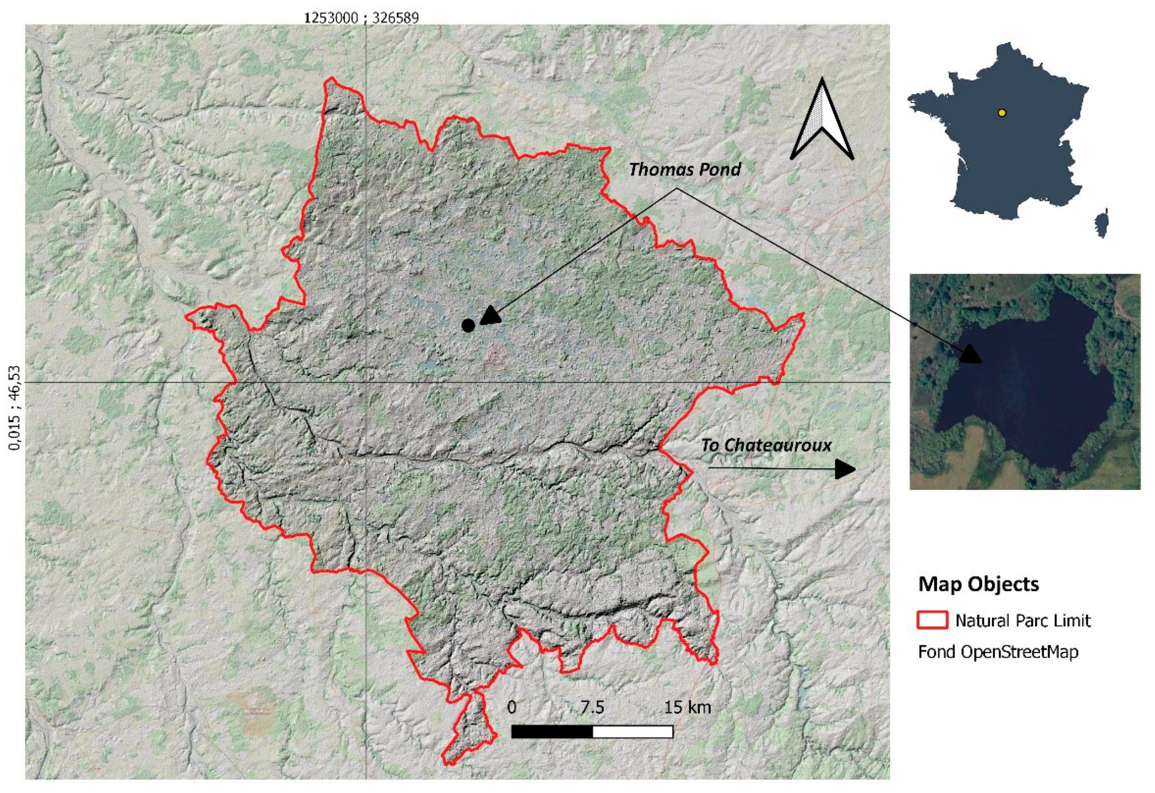
• Study area description

The words “exceptional” and “remarkably fragile” are well suited to describe the landscapes of the Brenne Natural Regional Park, a wetland of international importance classified as a Ramsar site since 1991. It is marked by a considerable presence of medium and small-sized ponds with a high density. The park has nearly 4500 ponds spread throughout the territory, most of which are used for aquaculture, recreation and leisure (Figure 1).

Due to the abundant presence of ponds, the Brenne is known as the “Land of the thousand ponds”. It is one of the most extensive continental French wetlands of this type. Located in the department of Indre (36), 25 km at the west of Châteauroux, the park benefits from a relatively flat topography dotted with small flat-bottomed basins and predominantly clayey-sandstone geology that favours the storage of runoff water.

Three ponds were monitored for physicochemical and climatic parameters from January 2017 until September 2020, within the Foucault Massé nature reserve. Only the Thomas Pond was selected for this study due to its high similarity with the other two. The study site is located between 46.721706° and 1.225791. is the Brenne Park is located upstream of the Loire basin, and ialso houses several small watersheds. The Brenne Park extends over 10 ha with an average altitude of 105 m. The park has a degraded continental climate with a substantial oceanic influence. The average temperature varies around 11 °C, and the average annual rainfall is around 700 mm (655 mm in Mezière en Brenne located at 15–20 km north). The average depth of the ponds is between 1.5–2 m, and their average level variation per year is around 1–1.25 m (fluctuations estimated from the 2.5 years of measurements). The ponds are emptied periodically for cleaning purposes, and a monk controls their flows. The average flow rate of ponds varies around 5 × 10⁻² m³/s with a maximum of 1–2 m³/s during rainy periods.

• Materials

We selected one pond (Thomas Pond) out of the three hourly monitored ponds over the January 2017–September 2020 period. The hourly measurements accurately capture all of the variations of the main physical parameters related to the water mass.

For climatic measurements, three meteorological stations of the Vantage Pro 2 type were installed around the pond area within a radius of 10 km. The recording of 9 parameters at hourly time steps has started in 2016 and continues till now. The parameters include temperature, precipitation, humidity, wind (speed and direction), solar radiation, solar energy, reference evapotranspiration, and atmospheric pressure.

In parallel to the above-mentioned measurements, additional monitoring of intra-limnic physical parameters was also performed to identify the processes that occur in the water mass and control natural evaporative losses. Thus, thermal and water-level measurements were performed using Tyntag Aquatic 2 probes (Gemini Data Loggers UK, Chichester, UK) with a 10K NTC Thermistor sensor covering the measurements ranging from −25 °C to +70 °C with a resolution of 0.01 °C. For each pond, probes were placed at three depths (bottom, middle and at the surface) on a fixed pole planted in the centre of the pond, far from the monk, to avoid any turbulence that could disturb the global dynamics. The water level was monitored with an Xtroll type probe (In-Situ USA—Fort Collins, CO, USA and saler: SDEC France—Rousset, France) without atmospheric pressure compensation. Water-level data was corrected using the pressure data recorded by the weather station.

• Methods

We used several evaporation models to explain the thermal processes occurring during the year. In essence, we aim to understand the thermal dynamics of this water mass, specifically, the process of energy stock constitution and losses by direct evaporation. Two processing steps were necessary. The first one was the evaluation of the degree of energy replenishment within the water, and the second the evaluation of the consumption of this same energy through evaporation (the removal water fractions by transfer into the atmosphere). The models used in this study can be grouped into three main classes: (1) temperature-based models, (2) radiation-based models, and (3) mass transfer-based models. The first two groups allow the calculation of ET° evapotranspiration, and the last one computes evaporation by using decomposition, which gives rise to 3 sub-groups: (1) aerodynamic models, (2) combined models, and (3) energy balance.

A more contemporary approach, arising from the emergence of new models dedicated to time series that exploit the advantages of deep learning techniques by integrating methods such as CNN, ANN, and LSTM, was also used. Their application to environmental data prediction (ET°; reference evapotranspiration) has significantly improved the accuracy of results. Thanks to its effectiveness in different areas, several researchers have used the LSTM model [28]. These recent techniques have emerged with the increase in data size, giving rise to BigData. Many authors have used these new techniques [29] for evapotranspiration estimation and prediction.

This study applies a simple deep learning stacking ensemble model, using a similar approach to [27,28] for estimating and predicting ET°. The algorithm developed using Python takes advantage of powerful libraries such as Pandas [30] and NumPy [31] for the preprocessing steps of the data. The model is built using the Keras [32] library, and the results are plotted for observation using the Matplotlib [33] library.

We first defined the dataset by splitting it into a training and a test set, respectively. The training set includes 80% of the total values, while the remainder 20% is in the test set. The stacked ensemble model includes a first model composed of three LSTM layers, and each is separated by an activation (Swish [34]) and a dropout layer (to avoid overfitting). We close this first model using a dense layer that includes a ReLU (rectified linear unit) activation function (similarly to the input layer). The second model comprises four different Conv1D layers, each followed by a MaxPooling1D layer. Then, a flatten layer and two dense layers allow for closing of the model. The output of both models is then concatenated into a dense neural network composed of three dense layers and a dropout one after the first layer. The stacked ensemble model is then compiled using the “Adam” optimiser, and the mean squared error is selected as the metric to compute the loss function. The model is then fitted for 250 epochs with a batch size of 512.

A general illustration of the stacked model applied in this research is summarized as follows (Figure 2).

Before the short-term prediction using deep neural networks, we used a series of 14 models to estimate evaporation for the Thomas Pond.

The quantitative approach taken by this study to estimate evaporation losses is based essentially on empirical models. Those models take into account, partly, physical parameters (aerodynamic model: Equations (1)–(9)) and integrate meteorological factors that play a significant role in this process, such as with combined models (Equations (10)–(13)). In order to validate the results, the set of models was completed by using energy balances. The equations used are summarized in

Table 1. Summary of formulas used for the calculation of evaporation (at the Thomas Pond).

	Hydrodynamic Models
(1)	Hefner	E = 0.26 (1 + 0.54 u) (es − ea)	In/Day
(2)	Dalton [9]	E = 0.26 (1 + 0.54 u) (es − ea)	In/Day
(3)	Harbeck	E = 2.909 As − 0.05 u (es − ea) 0.88	In/Day
(4)	Holman	E = 0.8 (0.37 + 0.0041 u) (es − ea) 0.88	In/Day
(5)	Smith (1993)	E = (0.76(0.08893 + 0.7835 u) (es − ea))/hfg
(6)	ASHRAE	E = (0.08893 + 0.7835 u) (es − ea))/hfg
(7)	EPRI	E = (9.2 + 0.46 W2) (es − ea)	W/m2.
(8)	Sol Engi	Qevap = 9.15 KE (es − ea)	W/m2.
(9)	MTC	E = 0.00338 A − 0.05 + u × (es − ea)
	Combined Models
(10)	Penman Model	$Ep=\frac{\Delta }{\Delta +\mathbf{\gamma }}\mathit{R}\mathit{n}+\frac{\gamma }{\Delta +\mathbf{\gamma }}\mathit{E}\mathit{a}\mathit{p}$ With:Eap = 0.26 (1 + 0.536 u) (es − ea)
(11)	Penman-Monteith	$E{T}_0=\frac{0.408\Delta (R_n-G)+\gamma \frac{900}{T+273}{U}_2(e_a-e_d)}{\Delta +\gamma (1+0.34U_2)}$
(12)	Priestly and Taylor [32]	Ep-T = β[(∆/(∆ + γ)) × (Rn/λ)]
(13)	De Bruin Model	$E=\left(\frac{\mathbf{\beta }}{\mathbf{\beta }-\mathbf{1}}\right)\left(\frac{\gamma }{\mathit{D}+\mathit{\gamma }}\right)\mathit{F}\left(\mathit{u}\right)-\mathit{e}\mathit{s}-\mathit{e}\mathit{a})$ With:F(u): 2.9 + 2.1 u
	Energy Balance
(14)	Energy Balance Model	αsQSolar + εQsky + QCond = Qconv + Qevap + Qwater + Qadvected

.

• Aerodynamic models

For properly estimating the water deficit caused by the ponds of the Brenne Park to the rivers and, on a larger scale, to the whole Claise basin (one of the main tributaries of the Loire), several evaporation models were tested. Among these, aerodynamic models are considered by many researchers as being purely physical and not integrating (or only slightly) geographical factors (e.g., morphology of the ponds, water bodies, slope, land use, geology). Aerodynamic models are derived from mass transfer theory based on Dalton’s law, and assume that equation E = f(u) (es − ea) expresses evaporation from a surface into the atmosphere. These equations provide the direct evaporation rate that would be translated into energy using the following equation: Qevap = E_pρwh_fg. The calculation of h_fg is carried out using the following Equation (3): h_fg = 3.501 − 0.002361Ts.

The last model (MTC) distinguishes itself by incorporating areas, an essential morphological element that accounts for the absence of geographical factors in the other models. MTC models have the particularity of incorporating additional factors that may play an essential role in the evaporation process.

• Combined models (Table 1, Equations (10)–(13))

In order to assess evaporation using combined models, we selected three models: Penman, Priestly and Taylor, De Bruin. We consider these models to be robust based on their worldwide use and their integration of specific factors that play a crucial role in evaporation processes. They simultaneously combine the advantages of mass transfer methods, which are aerodynamic in nature, and the methods related to energy budgets. Direct evaporation measurements using a Bac Colorado were made on ponds located in the Chérine nature reserve in Brenne (a few kilometres further north). The measurements give values very close to those collected by the automatic station (Vantage Pro 2) installed since 2016 around the Thomas Pond.

• Penman Model (Table 1, Equations (10) and (11))

The Penman model, derived from physical processes, and widely used, has a substantial advantage that comes from the combination of the aerodynamic and energy balance models. Numerous researchers have demonstrated the effectiveness of this model for water bodies [6,7,19,27]. Ref. [28] proposes an equation dedicated to the estimation of water body evaporation (E), based on Dalton’s law “E = (es − ea) + f(u)” [4]. The latter represents the evaporation rate per unit time.

We also used the Penman-Monteith equation (Table 1: number 11), which we consider as a combined model formulated differently and which calculates the reference evapotranspiration ET°. This equation gives the reference evapotranspiration rate (ET°) for different land-use types.

• Priestly and Taylor model (Table 1, Equation (12))

This model, also derived from Penman’s combined model, was proposed in 1972. It is applied to wet surfaces that have the necessary conditions for evaporation. It is distinguished by the cancellation of the aerodynamic component and the multiplication of the energy component by 1.26. This factor (β) tends to 1.26 for relatively large and wet sites [35,36].

• De Bruin model (Table 1, Equation (13))

Known as a combination of the two previous models (Priestly-Taylor and Penman), it distinguishes itself by its simplicity due to its use of three simple and accessible climate parameters (air temperature, wind speed and relative humidity). Proposed in 1978, this model gives the evaporation rate using the equation in Table 1: Equation (13).

The three previous models, belonging to the combined models, tend to gravitate around the Penman equation by making some modifications and combining both aerodynamic and energetic models. However, some factors of geographical nature that can influence the calculations and consequently the evaporation rates are not considered, thus making these models purely physical ones. According to [37], direct measurements of climatic parameters summarizes the geographical factors.

• Energy balance model (Table 1, Equation (14))

This model focuses on the water-air interface and the energy balance that benefits this water body area. Therefore, the energy received is equal to the energy emitted by the different processes at this interface. The heat exchange of the different energy sources in a pond can be summarized according to [20,38] 1968 equation (Table 1, Equation (14)).

It is a direct application of thermodynamics law, which estimates the excess or deficit of energy in the water body. Engstrom, in 1920 assumed that this method, known as the “energy budget method”, is based on the conservation of energy in the water mass. The input is, therefore, from solar radiation (short wave radiation), conduction, and condensation. Conversely, the loss is caused by evaporation, conduction, advection, and reflected radiation.

3. Results

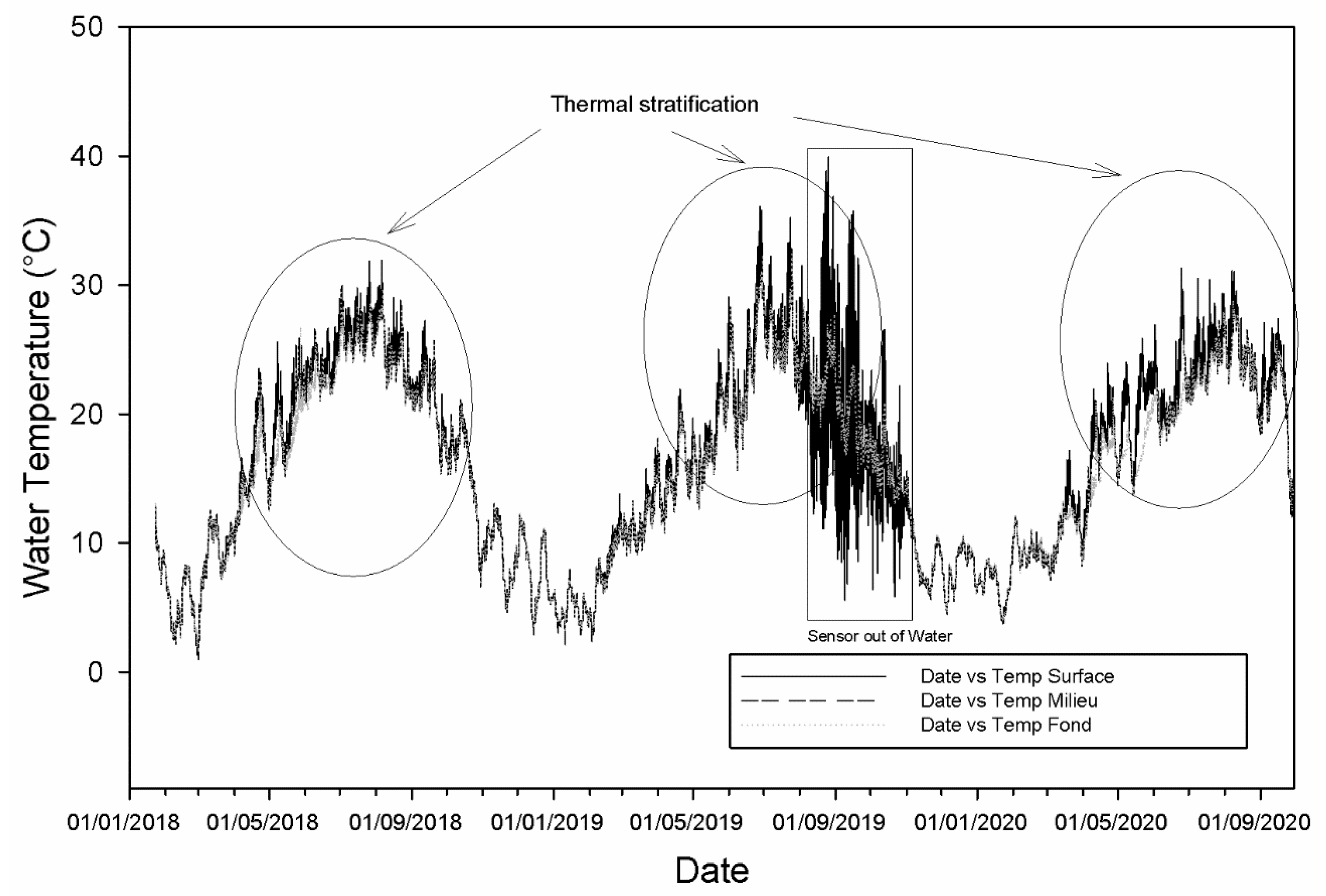
3.1. Thermal Variations of Water Body

3.1.1. Analysis of Thermal Variations of Water Masses over the Measurement Period

The regular monitoring of pond water temperatures at three depths confirms a close relationship between air and water temperature, especially in surface waters. This phenomenon tends to decrease slightly with depth. The graphical representation of water temperature of the epilimnion layer data, recorded at Thomas Pond over the 2018–2020 period, shows a thermal variability that is strongly conditioned by climatic factors (mainly air temperature) and partially by water inputs from surface and subsurface runoff or precipitation. As shown Figure 3, seasonal effects are evident, we observed a significant increase in temperatures during the summer period, reaching maximums of over 30–35 °C. On the other hand, a very marked decrease during winter season reaching temperatures in the order of 2 to 3 °C results in an annual thermal amplitude of 31 °C. The variations recorded for small temperatures (a few degrees 2:4 °C with resolution of 0.01 °C) are mostly related to short-lived showers, winds or frost.

3.1.2. Thermal Analysis of the Water Masses of the Thomas Pond

As numerous studies have demonstrated, watercourses show a very high correlation between water and air temperature. This correlation, often due to shallow water depth, implies that the morphology and dynamics of water bodies could induce a different thermal response directly impacting evaporation. In order to understand the physical processes behind this phenomenon, a comparative analysis of air and water temperatures proved to be a good compromise. The comparison was carried out on all three compartments of the water body. However, due to their direct involvement in the evaporation processes, only the surface measurements were considered. The comparative analysis of surface water and air temperatures shows a robust correlation between the two variables (r = 0.93) (Figure 4). However, this adjustment is not very effective since it does not consider thermal extremes, especially when we know that during the strongest thermal episodes, there are essential exchanges with the atmosphere by evaporation. This exchange rate reaches its maximum at the end of the reconstitution of the energy stock of the water mass, corresponding, in essence, to the end of the summer season.

The distribution of the observation points on the previous graph indicates that linear regression is not sufficiently suitable for measuring the correlation. Several approaches have been tested to find the best fit between these two parameters, and only the S-shaped function seemed to provide a satisfactory result.

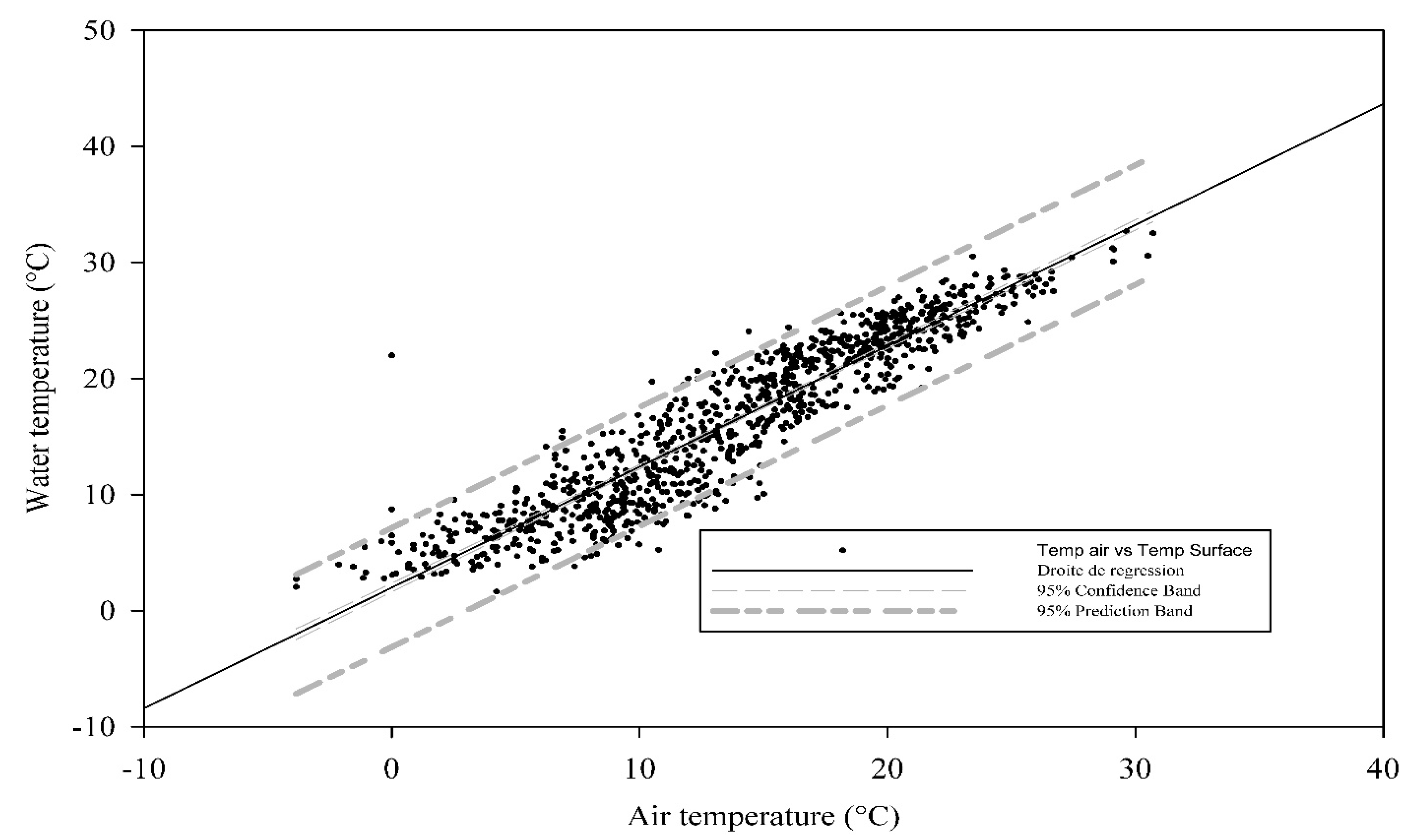
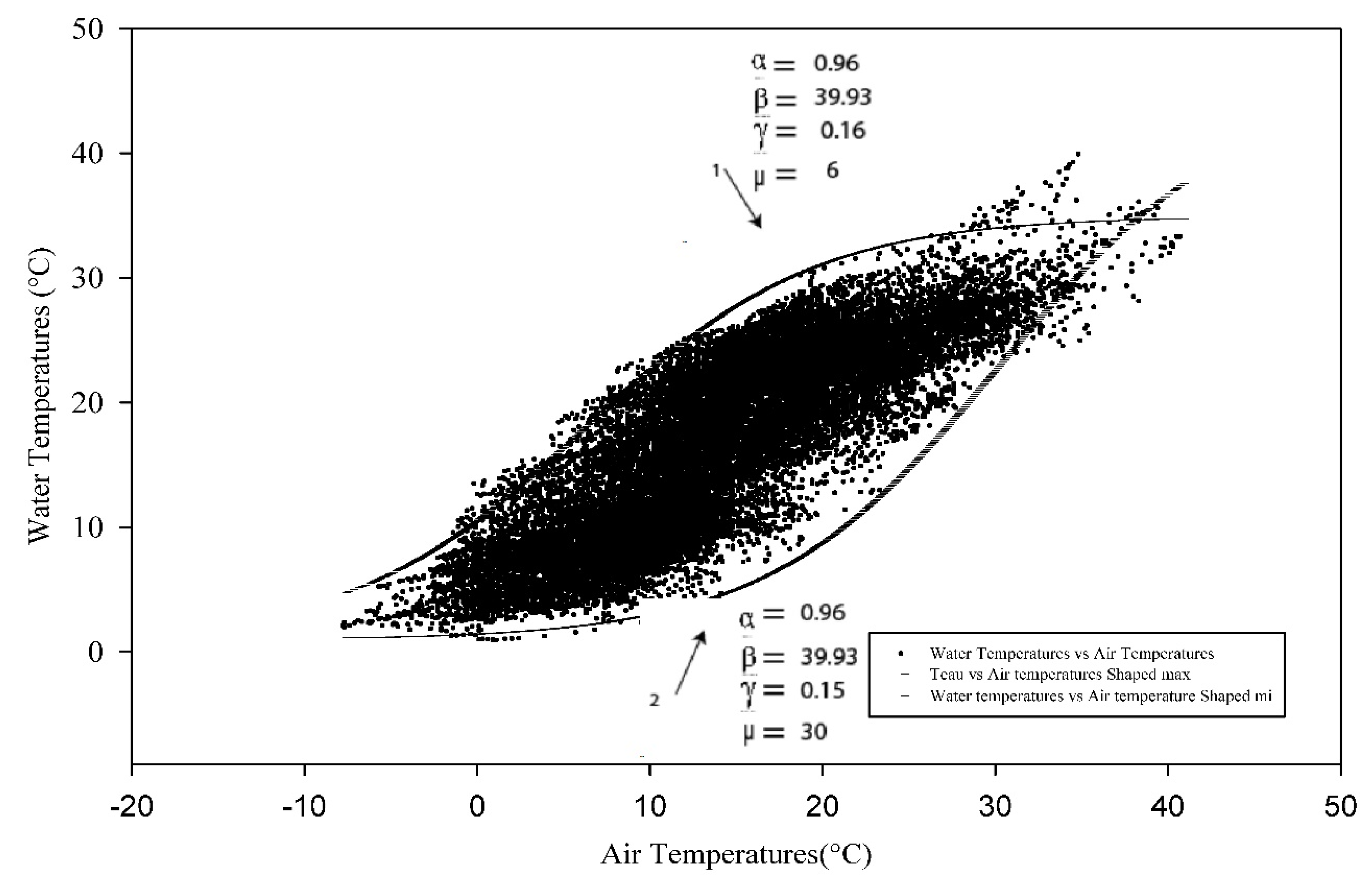
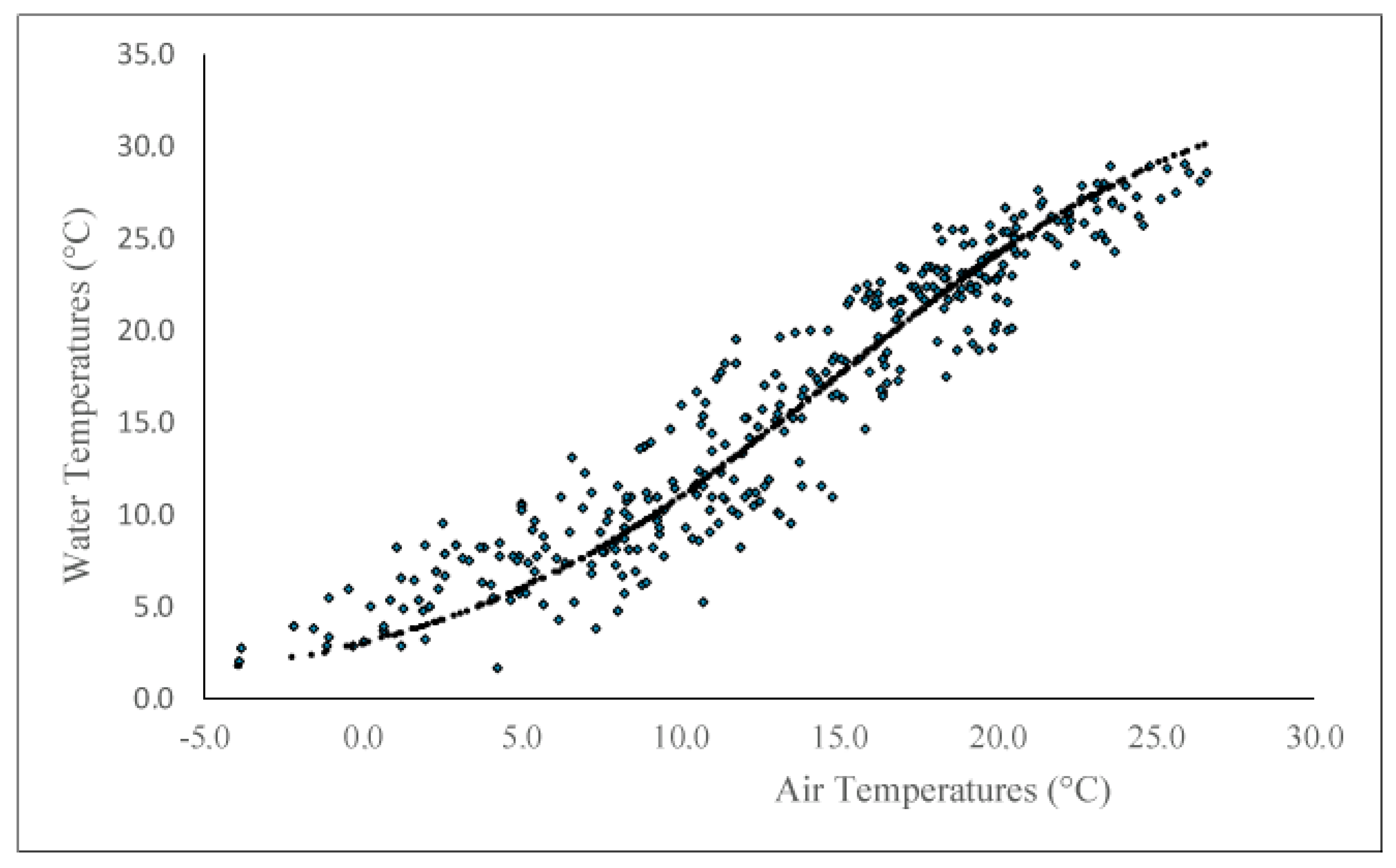
3.1.3. Adjustment of Air and Water Temperatures According to the S-Shaped Function

This first approach clearly shows the close relationship between air and water temperatures, but the linear model only explains 80 to 85% of the temperature variation. However, the differences observed are probably due to other morphological factors such as the topography of the watershed, the inflow-outflow, or climatic factors (precipitation, solar energy, …). This model could be suitable for thermal simulations in the context of climate change [21]. However, the low air temperatures of the winter period and conversely the higher temperatures of the summer period escape this exercise, making it difficult to predict the water temperatures at these periods. In order to better determine the degree of correlation between the two variables and to take into account all of the values, including the extreme values, we used a shaped function adjustment (Figure 5). The equation on which we based these adjustments is of type (1):

$$Teau=\mathrm{\mu }+\frac{\mathrm{\mu }-\mathsf{\alpha }}{1+\exp \gamma \left(\beta -Tair\right) }$$

where Teau, surface water temperature °C; Tair, air temperature °C; α, maximum water temperature (°C); β, air temperature at the inflection point; γ, slope of the function.

This adjustment was then applied to the daily averages (Figure 6) to evaluate better the thermal and, therefore, energetic variability of the water mass. The application of this law highlights several phenomena similar to what has been demonstrated by [19] for river temperatures.

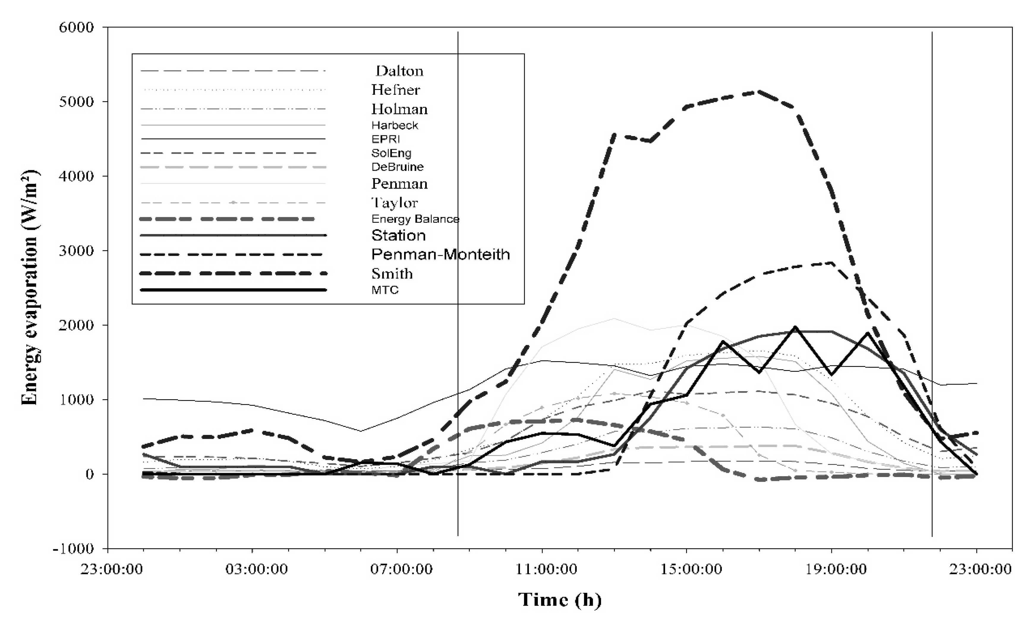
3.2. Estimation of Evaporation and the Energy Consumption Induced by This Process

The statistical synthesis of the evaporation energy of the 14 models used (

Table 2. Statistical characteristics of the evaporation energy calculated using different methods.

	Dalton	Hefner	Holman	Harbeck	EPRI	SolEng	DeBruin
Min	37.70	4.59	3.06	0.00	46.42	6.57	2.08
Max	126.45	971.77	392.39	1038.78	1275.06	621.90	343.45
Moyenne	48.67	186.80	81.09	129.76	496.81	165.24	57.73
	Penman	Taylor	Energy Balance	Station	Penman-Monteith	Smith	MTC
Min	5.78	0.00	−11.58	0.00	0.00	10.28	0.00
Max	830.48	334.62	298.42	885.45	1105.03	3086.85	2916.41
Moyenne	253.30	67.76	153.27	290.92	312.73	530.92	358.24

) shows us that, for the most part, the orders of magnitude are respected, as observed in the results obtained by other studies of the same type [33]. Values fluctuate between a minimum of 48 W/m² for the Dalton model and a maximum superior to 4000 W/m² for the Smith model. The Penman-Monteith and MTC models are relatively close to the results of the measuring station (average: 290–358 W/m²). The maximums can reach or even exceed 3000 W/m² for the Smith model, and the minimum is about 10, giving an average of 500 W/m², which is comparable to the Penman and MTC models. On the other hand, the aerodynamic models remain well below 200 W/m², which weakens the relevance of these models. We do not exclude that the presence of hydrophilic vegetation in the water body, which is not taken into account by the different models and would partially contribute to the variability of the results.

The graphical representation of daily evaporation energy rates for 2018 shows a variation between 50–3200 W/m² for most models, with aerodynamic models’ rates below 1000 W/m² (Figure 7). These values are in line with most results obtained by other researchers in the field.

We compared the calculated evaporation rates with those obtained by the measuring station and the Penman-Monteith formula to estimate the degree of adequacy and accuracy (Figure 8).

Only three methods show comparable rates (Smith, Penman, and MTC), highlighting the efficiency of the combined models. Incorporating the spatial dimension (area) in the Smith model could explain the closeness of these results to the combined models. The comparison of evaporation rates in 2018 with the difference in water level between the maximum and minimum level (90 cm) during the summer season, a period that we consider as uninfluenced (no inflow-outflow by concentrated or diffuse flow), highlights the relative effectiveness of the three methods (MTC, Penman-Monteith, and Smith) (Figure 9).

Correlation analysis of the different rates obtained using the 12 methods shows that, overall, the coefficients are very high for the aerodynamic models (Dalton, Hefner, Holman Harbeck and Smith) and, conversely, relatively low for the data from the measuring station and the energy balance (

Table 3. Correlation matrix of evaporation rates estimated using the different methods for the year 2018 at Thomas Pond.

	Dalton	Hefner	Holman	Harbeck	EPRI	SolEng	DeBruin	Penman	Taylor	Energy Balance	Station	Penman-Monteith	Smith	MTC	Delta Niveau (cm)
Dalton	1.00	0.94	0.95	1.00	0.60	0.79	0.92	0.66	0.58	0.27	0.08	0.07	0.97	0.14	0.10
Hefner	0.94	1.00	1.00	0.95	0.77	0.95	0.91	0.74	0.68	0.30	0.16	0.15	1.00	0.18	0.13
Holman	0.95	1.00	1.00	0.95	0.78	0.94	0.92	0.74	0.67	0.31	0.15	0.15	1.00	0.18	0.13
Harbeck	1.00	0.95	0.95	1.00	0.61	0.79	0.92	0.66	0.58	0.27	0.08	0.07	0.97	0.14	0.10
EPRI	0.60	0.77	0.78	0.61	1.00	0.85	0.59	0.71	0.62	0.31	0.26	0.25	0.74	0.23	0.18
SolEng	0.79	0.95	0.94	0.79	0.85	1.00	0.80	0.75	0.71	0.30	0.22	0.22	0.92	0.20	0.14
DeBruin	0.92	0.91	0.92	0.92	0.59	0.80	1.00	0.61	0.53	0.29	0.09	0.08	0.92	0.12	0.13
Penman	0.66	0.74	0.74	0.66	0.71	0.75	0.61	1.00	0.88	0.64	0.03	0.03	0.73	0.06	0.20
Taylor	0.58	0.68	0.67	0.58	0.62	0.71	0.53	0.88	1.00	0.68	0.05	0.04	0.67	0.10	0.16
Energy Balance	0.27	0.30	0.31	0.27	0.31	0.30	0.29	0.64	0.68	1.00	−0.17	−0.16	0.29	−0.08	0.14
Station	0.08	0.16	0.15	0.08	0.26	0.22	0.09	0.03	0.05	−0.17	1.00	0.98	0.14	0.76	0.18
Penman-Monteith	0.07	0.15	0.15	0.07	0.25	0.22	0.08	0.03	0.04	−0.16	0.98	1.00	0.14	0.70	0.16
Smith	0.97	1.00	1.00	0.97	0.74	0.92	0.92	0.73	0.67	0.29	0.14	0.14	1.00	0.18	0.12
MTC	0.14	0.18	0.18	0.14	0.23	0.20	0.12	0.06	0.10	−0.08	0.76	0.70	0.18	1.00	0.07
Delta Niveau (cm)	0.10	0.13	0.13	0.10	0.18	0.14	0.13	0.20	0.16	0.14	0.18	0.16	0.12	0.07	1.00

). The correlations with the combined models fluctuate between 0.70 and 0.97.

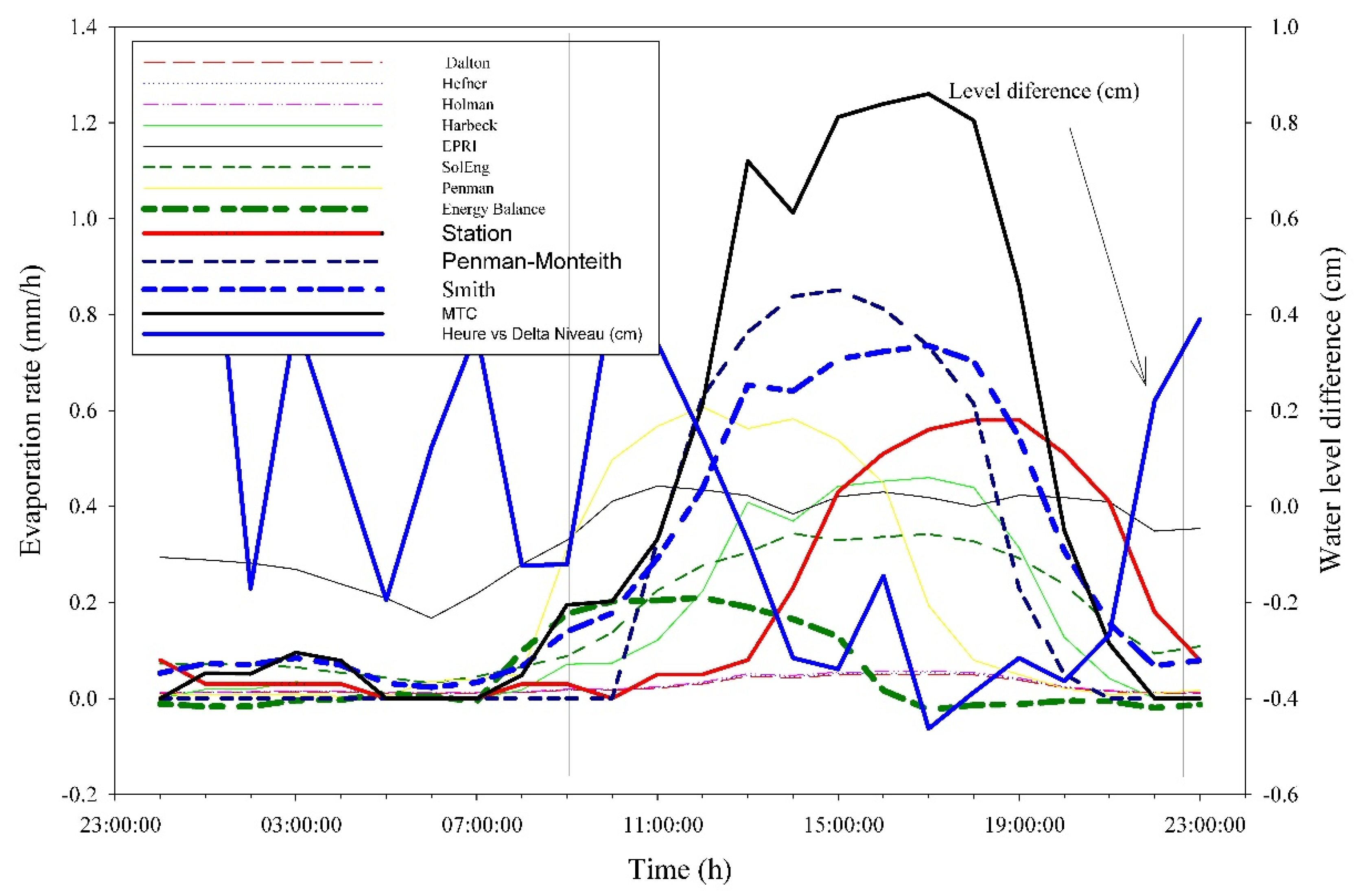
3.3. Appreciation of Daily Exchanges

Many authors have opted for a weekly analysis [8,18] which seems to be a reliable compromise to evaluate the energy exchanges between water and atmosphere. In order to report the method that appears to be the most suitable for our region, giving results that reflect the energy flows used by this process, and the amount of water evaporated, we selected 2 August 2018 as the most viable. This selection is based on several climatic and hydrodynamic factors (wind, precipitation, input-output). Precipitation rates before this date over fifteen days are almost zero. At the same time, the monk of the pond being closed and leaving no flow downstream makes the water body enter a phase of total isolation (with the only exchange being evaporation).

The Figure 10 shows that most of the energy mobilized occurs between 8:00 a.m. and 11:00 p.m. A plateau is reached at 1 p.m. and continues until 6 p.m., at which time we see an apparent cooling from a maximum of about 4800 W/m² for Dalton and slightly less for Penman to a value of fewer than 1000 W/m² in the space of 3–4 h.

The summer season in this region is known for its intensity. It involves closing the bungs/monks and stopping the flow to the tributaries that are adjacent to most ponds. As a result, inputs are minimal, first due to the low rainfall amounts/intensity and second due to the small size of the catchment areas of the ponds. The water is mainly lost through evaporation and/or evapotranspiration, which results in a steady drop in the pond levels throughout summer. This evolution is confirmed by the water level variation, which follows a few mm decrease between 8:30 and 22:00. We also saw a direct and substantial relationship between these two parameters. This observation confirms that mainly evaporation regimes over the waterbody. Moreover, it shows that no influence of surface and/or subsurface runoff participates in the hydrological dynamics of the water body during summer (Figure 11). Thus, as shown in the figure, any variation in level is accompanied by an inverse variation in evaporation.

First, we try to understand better the relationship between surface water temperature (upper layer of the epilimnion) and evaporation, and its impact on water-atmosphere exchanges. The graphical representation of these two parameters highlights several observations: (Figure 12).

-

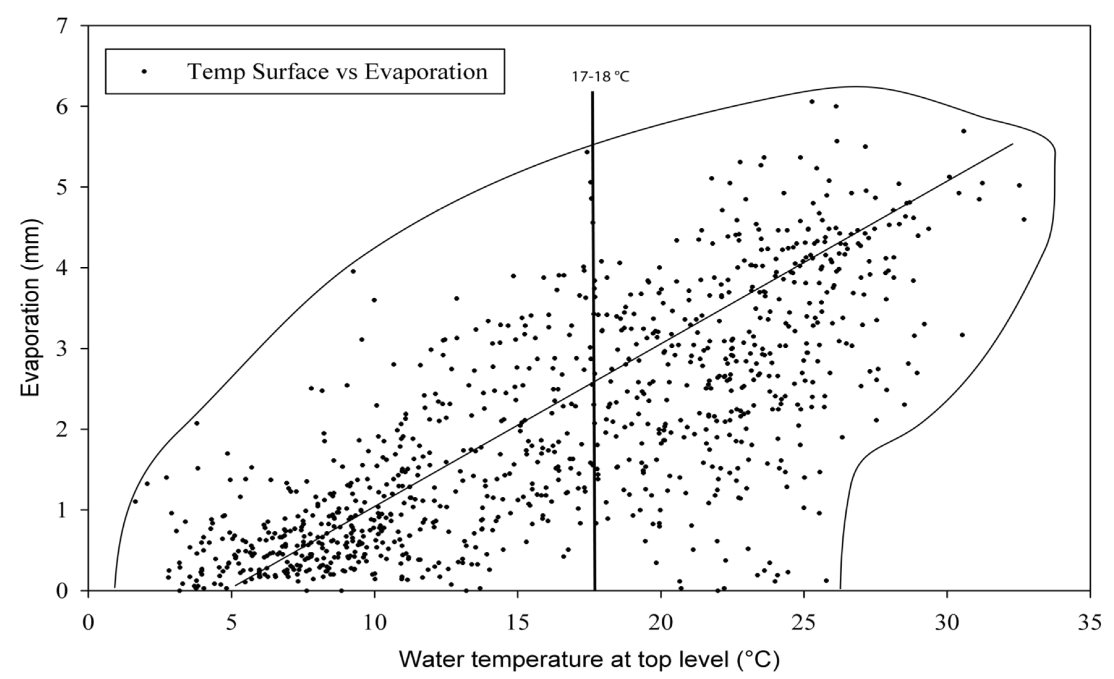
We observe a direct relationship between surface water temperature and evaporation. This relationship is much more visible for low water temperatures (winter period) and characterised by low exchanges with the atmosphere. During this phase, the reconstitution of the energetic stock of the water mass takes place. Conversely, it tends to increase with time until summer (water temperature varying between 12 °C and 25 °C). Very high temperatures tend to show relative evaporation stability around 3–5 mm. This stability probably indicates an over-saturation of the air with moisture and the low renewal of the ambient air. The low renewal rates might arise from the absence of winds or a reduction of its speed during most of this season.

-

The evaporation rates differ for the same water temperature and depending on the air temperature and, more precisely, the season. Thus, depending on whether the season is cold or warm, the same temperature is experiences different evaporation rates. The thermal energy stored in the mass is directly responsible for this effect giving rise to hysteresis. As shown Figure 12, the graphical representation of air temperatures and ET indicates that for the lowest temperatures and at the beginning of the energy stock reconstitution, the thermal amplitude is high for the same evaporation value. At an average temperature of 17.5 °C, the evaporation gap can vary from 1 to 6 mm.

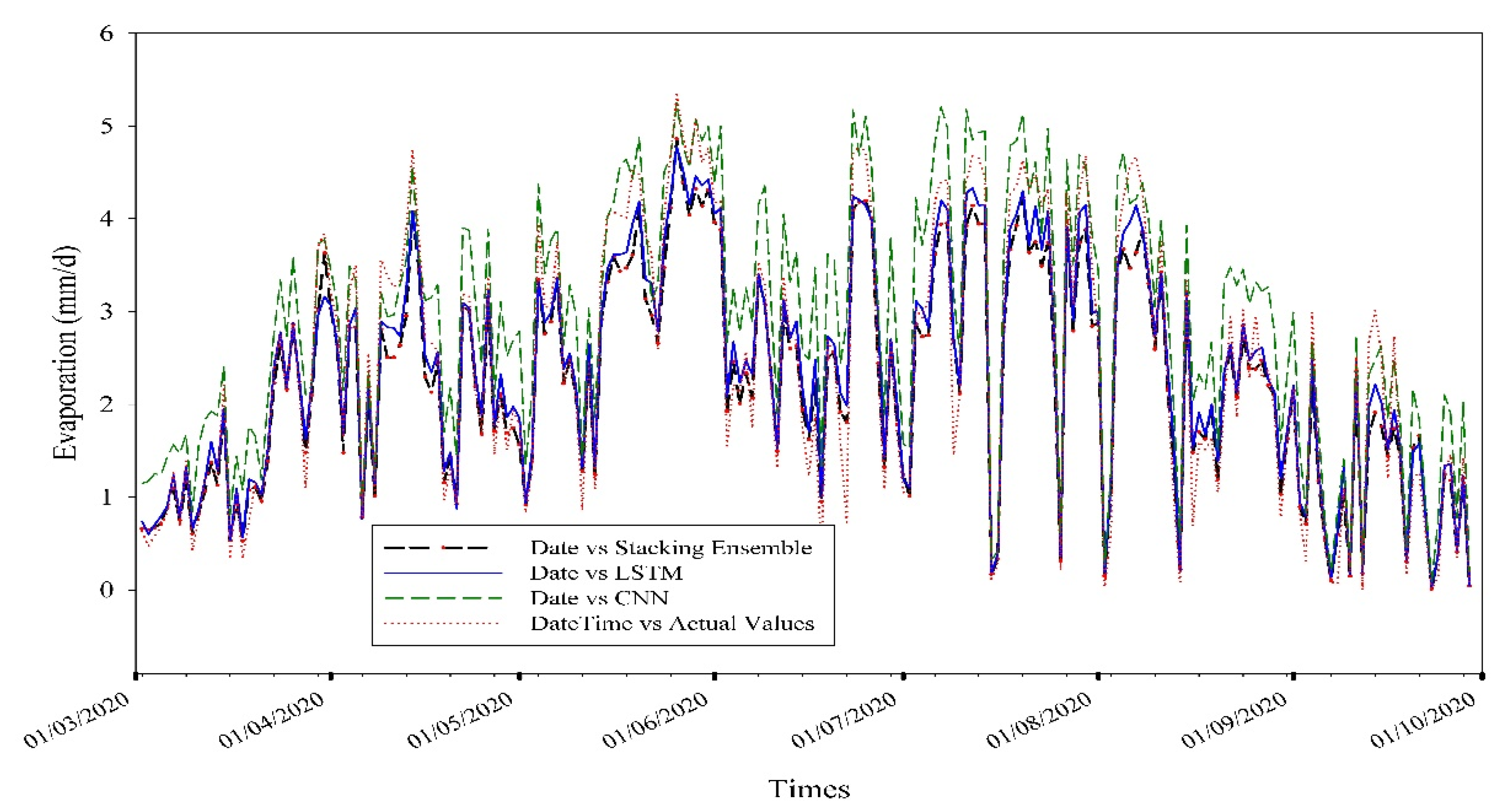
3.4. Prediction Using Deep Learning Methods

The application of the two methods, namely CNN and LSTM, in their basic form and, in a second time, their assembly by the reintegration of the first level results, allows for several observations. Two stages were necessary to apply the models, a training phase which requires a sufficient volume of data to calibrate and adjust the model, followed by a prediction phase which covers a relatively short period if we want to obtain results with sufficient accuracy. For this purpose, we used hourly measurement data covering the years 2018 and 2019 to model evaporation with the basic models and then integrate the latter’s results into an ensemble level model to produce a more accurate final result.

In their basic form, the CNN method tends to overestimate evapotranspiration, giving deviations in the order of 0.2 mm (Figure 13) from measured data.

On the other hand, LSTM displays very close results to the station measurements with deviations below 0.03 mm, giving this method excellent reliability.

Combining the two primary methods in a second step further refines the prediction and considerably reduces the deviations. Thus, the calculated error varies around 0.007, which is relatively low. The analysis of the deviations shows that the overall model tends to slightly underestimate evapotranspiration, while remaining very reliable in its prediction.

Using the scikit-learn library [38], we measured the mean squared error regression loss (RMSE) between the data measured by the station, the LSTM model, the CNN model and the ensemble stacking model. The RMSE obtained are 0.003944, 0.006364, and 0.004141 for the CNN, LSTM, and stacking ensemble models. Further research should help determine a better model to apply t and to verify if the CNN model may have some positive effect that is not detected through the calculation of the RMSE.

3.5. Extended Water Storages Recorded during the Last Two Decades Reflect the Deficit Caused by Direct Abstraction by Evaporation: Prediction of Sustained Shortage under Rising Temperatures

The alarming observations of water deficit in the ponds, issued from a regular monitoring of water levels, highlight strong evidence of losses by evaporation. In this vein, the most influencing factor that supports the involution hypothesis is water temperature, which in turn is influenced by air temperature (R² = 0.86). Based on this relationship, and on the forecasts of the IPCC’s optimistic and pessimistic scenarios, we wanted to assess this deficit in order to measure its overall impact on the Claise basin, and more broadly on the contribution of the Brenne’s ponds to the Loire. In collaboration with the Brenne Natural Park, an inventory of water bodies was carried out in 2014–2016, and a geographic information system was set up using ArcGIS (10.3) to highlight all of the characteristics of these water bodies. In total, 4500 ponds are present on the territory of the park. Evaporation rates calculated by the Penman-Monteith equation, are the closest to values observed by in-situ measurements in the north of the Chérine reserve. Therefore, the Penman-Monteith-derived values were subsequently used. For this purpose, we took data from the weather stations present on site (2018) and applied the temperature increase scenarios projected by the IPCC.

In order to estimate the volumes of water lost through direct evaporation, the total surface area covered by the ponds in the park was calculated by aggregation. Given the different results obtained previously and with a total of 4500 ponds in the park, the direct water losses would contribute to a relatively significant lack of water which is translated by the drying of watercourses very early in the year, even before summer. The dry phase of these rivers is of four to five months/year. During summer, the ponds engage in a phase of increased exchanges with the atmosphere, thus losing an average of 4700 mm during four to five months and a total of 700 mm/year. These losses cause drastic decreases of water volumes, in contrast to sharp increases of temperature and stocked energy. During this period, the ponds are hydrologically isolated, receiving few or no water from the slopes of their small catchment areas. They seem to be closer to reality for a cumulative surface of the park’s ponds of about 7666 Ha. As we can see, in 2018, the average loss was about 57,281,941.3 m³. Considering the optimistic and pessimistic climate scenarios put forward by the IPCC reports, estimated at a rise of between 1 °C and 4 °C, the results obtained show the extent of the shortage and, consequently, the water deficit that the Claise River will suffer in the coming years (

Table 4. Evolution of the volumes (m³) of water exchanged with the atmosphere by evaporation according to the IPCC scenarios on all of the water bodies of the Brenne Park.

Methods\Volume Evaporation at Temp °C	Current	1 °C	2 °C	3 °C	4 °C
MTC	656,996,80.2	698,356,98.3	741,889,20.5	787,780,45.1	836,138,17.8
Penman-Monteith	544,286,00.00	558,940,27.5	573,514,13.79	588,383,72.2	603,569,64.93

). It is therefore undeniable that the combination of water volume reduction and temperature increases during summer significantly increases stocked energy, hence promoting further losses by evaporation. This observation indicates that that water of the ponds can only be preserved by extending the closure period of the monks. However, this process leads to the drying of the streams associated with the ponds. The state of water deficit in the Claise basin, and more broadly of the Loire, is hence amplified.

The monitored temperatures for the ponds do not allow us to confirm or deny the impact of climate change on the hydrological balance of these ponds and, more broadly, of the Claise River basin. Nevertheless, the traces of certain hydrological phenomena (drying up of associated watercourses over long periods, consequent drop in the level of water bodies and the drying up of certain small ponds, etc.) reinforce the hypothesis that a direct climatic impact cannot be excluded.

4. Discussion

In contrast to many studies that address evaporation and its effect on the water balance of watershed, the effect of evaporation on limnic settings remains rare and poorly documented. The close density and the abundance of these waterbodies (ponds) complicate the assessment of evaporation due to the multitude of the involved factors. The comparison of air and water temperatures demonstrates the presence of a relatively strong relationship between these two factors (similarly to rivers). Nevertheless, this relationship is subjected to a second factor, that of energy stocks, that reinforces or reduces, depending on the season, exchanges with the atmosphere. As such, the meticulous analysis of energy stocks and their dispersion gives a good idea of the staggering losses by evaporation. Two time scales were considered, namely the short scale (day) and the long scale (year), to try and understand the processes (day-night effect) and (seasonal effect). The estimation of this parameter using several equations (models) gives different results, hence the difficulty in its approach. The direct measurements we made near the site using a Colorado pan converged with the results obtained using the Penman equation (Table 1, Equation (12)), programmed into the weather station (Vantage Pro2). The large variability of the estimated rates results from a combination of many factors related (mainly) to the climate and the geography of the ponds and their watersheds. The evolution of the recorded evaporation rates is directly related to the stock of energy stored by the water mass, giving rise to the hysteresis phenomenon. Two energy stages that generally condition evaporation should be considered: First on the daily scale where we witness the beginning of exchanges with the atmosphere. These start at 8–9 a.m., peak around 3–4 p.m., and drop to their minimum around 7 p.m. This warming phase depends on the volume of energy stored by the water mass, which reaches its maximum during the summer period and that is considerably reduced during winter. This accumulation is mainly due to radiation and probably surface runoff (mainly from tributaries). It is also possible that some of it comes from chemical reactions (exothermic ones), but this is negligible. Estimating the amount of energy stored in the mass using different formulae gives variable results ranging from 400 W/m² for some hydrodynamic models to over 4000 W/m². The results of several studies give comparable values, falling into the low range < 1500 W/m².

The summer season, known for its prolonged exposure to sun and day length, accentuates evaporation, resulting in a notable drop in the water level. During this period, net radiation reaches its maximum in July-August, and the energy stored in the water mass is generally higher than 1500 W/m², favouring the evaporation process. In parallel to these meteorological processes and during the summer period, the organisation of the water mass into three layers giving rise to thermal stratification. This distinction isolates the upper layer of the water mass, which is relatively warmer than the other layers of the water mass (metalimnion and hypolimnion) and would increase the exchange with the atmosphere (evaporation). The thermal stratification is very fragile and is effective for short periods, often disturbed by two climatic factors: wind and precipitation. These factors act directly by mixing the water mass, which reduces the temperature of the surface layer, leading to the loss of part of the energy stored in this layer.

In an attempt to assess the strength of this thermal (air-water) relationship, a correlative analysis was performed on the thermal data from Thomas Pond and confirmed on the data from Pifaudière and Neuf Ponds which will not be discussed in this analysis. The S-shaped fit confirms the high variability of the water temperatures, especially with the air temperature ranging between 10–25 °C, which can only be explained by the energy stock of the water mass. The application of the equation allows us to see that the cloud of points is framed by two curves of the S-shaped type, the first of which links the maximum temperatures and the second the minimum temperatures, between which fluctuate all of the temperatures acquired by the water mass during the year with different characteristics. The two curves form an envelope that reflects the hysteresis effect through which the thermal state of the water body passes during its annual thermal cycle and reflects the constitution and evolution of the energy stock. It, therefore, shows the periods during which the evaporation process reaches its maximum, consuming a large part of the stored energy. The entry of the water body into a cooling phase leads to its progressive mixing by energy loss, which results in a single thermally homogeneous layer with an average thickness of 2.5 m. This homogenisation results in a decrease in energy storage and exchanges with the atmosphere (evaporation).

The daily evaporation rates for the year 2018 show a remarkable seasonal effect globally in adequacy with the evolution of the level of the pond during the summer period, where the water body enters a phase of isolation and where the evaporation remains the principal factor of exchange with the atmosphere (Figure 8). The effects of evaporation begin to be felt as early as February, with rates fluctuating around 5 mm/d for models that overestimate this phenomenon (mainly Taylor). The spring, summer and autumn seasons are characterized by much higher rates for all models, with relatively disparate orders. The latter varies between a maximum during July and August. The rates can reach 27 mm/d for specific methods, which we consider overestimated (making their calculation methods unsuitable).

The order of magnitude of evaporation for the year 2018 at Thomas Pond varies from 700 to 730 mm. The waves caused by the low winds could explain the differences in water level. Indeed, the amplitude of the level is 900 mm, to which we subtracted the rare contributions by precipitation (80 mm) and the contributions by surface and subsurface runoff that we considered weak but present. This calculation leads us to a comparison with withdrawals by evaporation.

It is important to note that the Smith model is part of the set of combined models and correlates well with the TCM (transfer coefficient model) and Penman-Monteith. As we have seen, the different combined models are all derived from the Penman equation, making it difficult to consider the results obtained by these methods. The correlation of the Smith model with the station data is very low, thus reducing its effectiveness for the sector. It should be noted that the Debruine model is not correlated with any of the data from the different models and shows a negative correlation with the station results.

The global analysis of energy at an hourly time step does not allow to observe the results of the different methods and to appreciate with precision the evaporation process as well as the energy mobilized either from the energy stock of the water mass and/or from that produced by the solar radiation. The thermal amplitude decreases considerably at high temperatures and the end of the energy cycle, coinciding with the summer and autumn periods.

The warming of the upper layer of the water mass becomes effective from 8:00 and reaches its maximum in the middle of the afternoon. This process enters a cooling phase from 21:00–22:00, thus reducing the energy input to the water mass. Thanks to its storage capacity, the water mass reconstitutes its stock during this period. Exchanges with the sediments cannot be excluded due to the thinness of the water mass, a fact confirmed by the thermal sensors installed at depth which show differences between the surface and bottom temperatures during the stratification period.

A two-stage prediction: this first phase of prediction using deep learning models gives excellent results in the short term but remains insufficient if we want to obtain a vision close to reality in the medium and long terms to assess the effect of temperatures rise. This method will help predict the short-term evaporation needed by managers to regulate flows and/or combat water losses. Indeed, these losses likely disrupt both the hydrological dynamics of the water body, its tributaries and, more broadly, the hydrological balance of the Claise and Loire catchment areas.

The second phases dedicated to simulate the evolution of water stocks under the new climates’ conditions given by the GIEC for the next century leads to the conclusion that both models show a significant increase in water withdrawal by evaporation under the constraint of an increase in air temperatures of 1 to 4 °C. The MTC model shows the highest increase, which is around 2 × 10⁶ m³, whereas Penman, which we consider to be the most suitable model for our region due to the adequacy of the results with the drop in the water level of the water body monitored, shows a more moderate increase of around 1.6 × 10⁶ m³ for the most pessimistic scenario. On the other hand, we must not lose sight of the fact that the water bodies ensure the maintenance of flows in the watercourses associated with the water bodies through regulation of flows by the managers.

5. Conclusions

The particularity of the Brenne is its limnologically rich setting region and its climatic setting characterised by a mild and cool climate in summer. This regime is strongly owed to the presence of numerous bodies of water (ponds) dedicated to aquaculture on the one hand and to irrigation on the other. The last few decades have seen the emergence of the problem of water resources, which leads managers and owners to retain water by closing bungs/monks over long periods. This behaviour leads to the drying up of many tributaries, directly impacting the larger Loire basin.

The regular monitoring of water bodies subject to a continental climate with a significant oceanic influence gives a better account of the disturbances of the withdrawals at different time steps. Estimating evaporation using different models tends to answer the question of the involvement of these water bodies in this process of resource reduction and especially the disturbance of the hydrological balance at all scales. The analysis of thermal data collected at hourly time steps during three years (2017–2020) and meteorological data (2016–2020) shows that the temperatures of the water bodies are directly impacted by the variations of the air temperatures and the energy stock of the water mass. Thus, the extreme values do not obey a linear relationship between the two parameters and are conditioned by the energy stock of the water mass. An adjustment according to a S-Shaped function highlights a phenomenon of hysteresis. This phenomenon reflects two fundamental elements: the stratification starting in April and ending in October, along with increased evaporation and the significant variability of the energy stock, which begins to rebuild during the same period. The use of several models for the estimation of evaporation has shown that the combined models are the most suitable for our region, giving values close to the measuring station’s results (~750 mm/year). These losses byevaporation is of the same magnitude as the water level differences during the summer season. The calculated evaporation energy shows values ranging from 40 W/m² for the essentially physically-based aerodynamic models to > 4000 W/m² for the combined models. The efficiency of these models probably lies in their integration of physical factors measured directly on-site (T°, wind, humidity). Only the Smith model integrates the surface, which could explain the closeness of its results with those of the combined models. Predictive modelling using deep learning models (CNN and LSTM) and their combination in an ensemble model gives relatively precise predictions, efficiently anticipating changes in the short term. In order to anticipate changes in the medium and long term and undertake management adapted to future climate conditions, the integration of IPCC scenarios contribute in some way to a better understanding of the impact of evaporative withdrawals and the imbalance in the water balance caused by these entities (ponds). A rise in air temperatures of 1 °C or 2 °C would lead to a loss of water for the Claise river and more widely for the Loire of around 50 × 10⁶ m³ on average, leading to a reconsideration of the current management model to anticipate the effects of future climate variations if we want to preserve the water reserves of the Loire and its tributaries.

References

1. Downing, J.A.; Prairie, Y.T.; Cole, J.J.; Duarte, C.M.; Tranvik, L.J.; Striegl, R.G.; McDowell, W.H.; Kortelainen, P.; Caraco, N.F.; Melack, J.M.; et al. The global abundance and size distribution of lakes, ponds, and impoundments. Limnol. Oceanogr. 2006, 51, 2388–2397. [Google Scholar] [CrossRef] [Green Version]
2. Potts, D.F. Estimation of evaporation from shallow ponds and impoundments in Montana. In Miscellaneous Publication N° 48; U.S. Department of Agriculture: Washington, DC, USA, 1988. [Google Scholar]
3. Bastiaanssen, W.G.M.; Cheema, M.J.M.; Immerzeel, W.; Miltenburg, I.J.; Pelgrum, H. Surface energy balance and actual evapotranspiration of the transboundary Indus Basin estimated from satellite measurements and the ETLook model. Water Resour. Res. 2012, 48, W11512. [Google Scholar] [CrossRef] [Green Version]
4. Zhang, Y.Q.; Chiew, F.H.S.; Zhang, L.; Leuning, R.; Cleugh, H.A. Estimating catchment evaporation and runoff using MODIS leaf area index and the Penman-Monteith equation. Water Resour. Res. 2008, 44, W10420. [Google Scholar] [CrossRef]
5. Enku, T.; Assefa, M.M. A simple temperature method for the estimation of evapotranspiration. Hydrol. Process. 2014, 28, 2945–2960. [Google Scholar] [CrossRef]
6. El-Mahdy, M.E.-S.; Abbas, M.S.; Sobhy, H.M. Development of mass-transfer evaporation model for Lake Nasser. Egypt. J. Water Clim. Chang. 2019, 12, 223–237. [Google Scholar] [CrossRef]
7. Luki, S.; Takehiko, F.; Yuichi, O.; Shigeru, M.; Takashi, G.; Ken’ichirou, K.; Shinya, H.; Hikaru, K.; Koichiro, K.; Tomomi, T. Analysis of stream water temperature changes during rainfall events in forested watersheds. Limnology 2010, 11, 115–124. [Google Scholar] [CrossRef]
8. Eaton, G.J.; Scheller, R.M. Effects of climate warming on fish thermal habitat in stream of the United States. Limnol. Oceanogr. 1996, 41, 1109–1115. [Google Scholar] [CrossRef] [Green Version]
9. Fukushima, T.; Ozaki, N.; Kaminishi, H.; Harasawa, H.; Matsushige, K. Forecasting the changes in lake water quality in response to climate changes, using past relationships between meteorological conditions and water quality. Hydrol. Process. 2000, 14, 593–604. [Google Scholar] [CrossRef]
10. Herb, W.R.; Stefan, H.G. Temperature Stratification and Mixing Dynamics in a Shallow Lake With Submersed Macrophytes. Lake Reserv. Manag. 2004, 20, 296–308. [Google Scholar] [CrossRef] [Green Version]
11. Prats, J.; Danis, P.-A. An epilimnion and hypolimnion temperature model based on air temperature and lake characteristics. Knowl. Manag. Aquat. Ecosyst. 2019, 8, 420. [Google Scholar] [CrossRef]
12. Culberson, S.D. Simplified Model for Prediction of Temperature and Dissolved Oxygen in Aquaculture Ponds: Using Reduced Data Inputs. Master’s Thesis, University of California, Davis, CA, USA, 1993; 212p. [Google Scholar]
13. Hondzo, M.; Stefan, H.G. Regional water temperature characteristics of lakes subjected to climate change. Clim. Chang. 1993, 24, 187–211. [Google Scholar] [CrossRef]
14. Hondzo, M.; Stefan, H.G. Lake water temperature simulation model. J. Hydraul. Eng. 1993, 119, 1251–1273. [Google Scholar] [CrossRef]
15. Bogan, T.; Stefan, H.G.; Mohseni, O. Imprints of secondary heat sources on the stream temperature/equilibrium temperature relationship. Water Resour. Res. 2004, 40, 1–16. [Google Scholar] [CrossRef] [Green Version]
16. Boyd, C.E. Water Quality in Ponds for Aquaculture; Auburn University Agricultural Experimentation Station: Auburn, AL, USA, 1990; 482p. [Google Scholar]
17. Boyd, C.E.; Romaire, R.P.; Johnston, E. Predicting Early Morning Dissolved Oxygen Concentrations in Channel Catfish Ponds. Trans. Am. Fish. Soc. 1978, 107, 484–492. [Google Scholar] [CrossRef]
18. Mohseni, O.; Stefan, H. Stream temperature/air temperature relationship: A physical interpretation. J. Hydrol. 1999, 218, 128–141. [Google Scholar] [CrossRef]
19. Mohseni, O.; Stefan, H.G.; Erickson, T.R. A non-linear regression model for weekly stream temperatures. Water Res. 1998, 34, 2685–2693. [Google Scholar] [CrossRef]
20. Water Resources Engineers, Inc. (WRE). Prediction of Thermal Energy Distribution in Streams and Reservoirs. In Report Prepared for the Department of Fish and Game, State of California; Water Resources Engineers, Inc.: San Francisco, CA, USA, 30 August 1968; 90p. [Google Scholar]
21. Robitu, M.; Inard, C.; Musy, M.; Groleau, D. Energy balance study of water ponds and its influence on building energy consumption. In Proceedings of the Eighth International IBPSA Conference, Eindhoven, The Netherlands, 11–14 August 2003. [Google Scholar]
22. Kroger, D.G. Evaporation-from a Water Suylface. Theor. J. Exp. J. 2007, 23, 3. [Google Scholar]
23. Sinokrot, B.A.; Gulliver, J.S. In-stream flow impact on river water temperatures. J. Hydraul. Res. 2000, 38, 339–349. [Google Scholar] [CrossRef]
24. Harbeck, E.G. For Measuring Reservoir Evaporation Utilizing Mass-Transfer Theory; Geological Survey Professional Paper 272-E; United States Government Printing Office: Washington, DC, USA, 1962.
25. Malik, A.; Kumar, A.; Kim, S.; Kashani, M.H.; Karimi, V.; Sharafati, A.; Ghorbani, M.A.; Al-Ansari, N.; Salih, S.Q.; Yaseen, Z.M.; et al. Modeling monthly pan evaporation process over the Indian central Himalayas: Application of multiple learning artificial intelligence model. Eng. Appl. Comput. Fluid Mech. 2020, 14, 323–338. [Google Scholar] [CrossRef] [Green Version]
26. Webb, B.W.; Clack, P.D.; Walling, D.E. Water-air temperature relationships in a Devon river system and the role of flow. Hydrol. Process. 2003, 17, 3069–3083. [Google Scholar] [CrossRef]
27. Wen, Y.; Yuan, B. Use CNN-LSTM network to analyze secondary market data. In Proceedings of the 2nd International Conference on Innovation in Artificial Intelligence, Shanghai, China, 9–12 March 2018; pp. 54–58. [Google Scholar]
28. Liu, S.; Zhang, C.; Ma, J. CNN-LSTM neural network model for quantitative strategy analysis in stock markets. In International Conference on Neural Information Processing; Springer: Berlin/Heidelberg, Germany, 2017; pp. 198–206. [Google Scholar]
29. Aseen, Z.M.; Al-Juboori, A.M.; Beyaztas, U.; Al-Ansari, N.; Chau, K.-W.; Qi, C.; Ali, M.; Salih, S.Q.; Shahid, S. Prediction of evaporation in arid and semi-arid regions: A comparative study using different machine learning models. Eng. Appl. Comput. Fluid Mech. 2019, 14, 70–89. [Google Scholar] [CrossRef] [Green Version]
30. Available online: https://pandas.pydata.org/ (accessed on 15 November 2021).
31. Available online: https://numpy.org/ (accessed on 15 November 2021).
32. Available online: https://keras.io/ (accessed on 20 November 2021).
33. Available online: https://matplotlib.org/ (accessed on 20 November 2021).
34. Ramachandran, P.; Zoph, B.; Le, Q.V. Searching for activation functions. arXiv 2017, arXiv:1710.05941. [Google Scholar]
35. Stewart, R.; Rouse, W. Simple model for calculating evaporation from dry and wet tundra surfaces. Arctic. Alp. Res. 1976, 8, 263–274. [Google Scholar] [CrossRef]
36. Mosner, M.S.; Aulenbach, B.T. Comparison of methods used to estimate lake evaporation for a water budget of Lake of estimation methods. Hydrol. Process. 1998, 12, 429–442. [Google Scholar]
37. Pallavi, K.; Rajeev, S. Evaluation of evaporation models based on climate factors. Int. J. Civ. Eng. Technol. 2016, 7, 111–120. [Google Scholar]
38. Available online: https://scikit-learn.org/stable/ (accessed on 22 November 2021).
Figure 1. Location of the studied ponds.
Water 14 00923 g001
Figure 2. Illustration of the stacked ensemble model used to predict ET° values.
Water 14 00923 g002
Figure 3. Changes in water temperatures between 2018 and 2020 at Thomas Pond.
Water 14 00923 g003
Figure 4. Correlation between air and water temperature (daily average) in the Thomas Pond.
Water 14 00923 g004
Figure 5. Adjustment of hourly (min and max) water temperatures as a function of air temperatures recorded at the Berger station in 2018.
Water 14 00923 g005
Figure 6. S-Shaped fit of 2018 daily mean water and air temperatures collected at the center of Thomas Pond (Brenne).
Water 14 00923 g006
Figure 7. Estimated daily evaporation energy by different methods from Thomas Pond for the year 2018.
Water 14 00923 g007
Figure 8. Estimation of daily evaporation rate by different methods from Thomas Pond.
Water 14 00923 g008
Figure 9. Daily evaporation rates determined using models with rates close to those of the Thomas Pond station for the year 2018.
Water 14 00923 g009
Figure 10. Evaporation rate on 2 August 2018 by different methods from Thomas Pond.
Water 14 00923 g010
Figure 11. Evaporation rate on 2 August 2018 by different methods from Thomas Pond.
Water 14 00923 g011
Figure 12. Evolution of evaporation with air temperature.
Water 14 00923 g012
Figure 13. Graphical representation of ET prediction results by basic and ensemble models.
Water 14 00923 g013