A GPU-Accelerated and LTS-Based Finite Volume Shallow Water Model

Abstract

This paper presents a GPU (Graphics Processing Unit)-accelerated and LTS (Local-time-Step)-based finite volume Shallow Water Model (SWM). The model performance is compared against the other five model versions (Single CPU versions with/without LTS, Multi-CPU versions with/without LTS, and a GPU version) by simulating three flow scenarios: an idealized dam-break flow; an experimental dam-break flow; a field-scale scenario of tidal flows. Satisfactory agreements between simulation results and the available measured data/reference solutions (water level, flow velocity) indicate that all the six SWM versions can well simulate these challenging shallow water flows. Inter-comparisons of the computational efficiency of the six SWM versions indicate the following. First, GPU acceleration is much more efficient than multi-core CPU parallel computing. Specifically, the speed increase in the GPU can be as high as a hundred, whereas those for multi-core CPU are only 2–3. Second, implementing the LTS can bring considerable reduction: the additional maximum speed-ups can be as high as 10 for the single-core CPU/multi-core CPU versions, and as high as five for the GPU versions. Third, the GPU + LTS version is computationally the most efficient in most cases; the multi-core CPU + LTS version may run as fast as a GPU version for scenarios over some intermediate number of cells.

1. Introduction

Shallow water models based on the Godunov-type finite volume method have been widely used in modeling urban/city/river/coastal flood disasters, tides, and storm surges in estuaries/nearshore regions, pollutants, sediment transport, etc. Examples include: Cea et al. [1], Hu et al. [2], and Luan et al. [3] for tidal flows; Qin et al. [4] and Kim et al. [5] for tsunamis; Kernkamp et al. [6] for tidal propagation on the continental shelf; Hu et al. [7,8] for coastal swash flows. However, the computational efficiency of such models is limited due to the Courant–Friedrichs–Lewy (CFL) condition on the time step, as well as the commonly used Global-Minimum Time Step (GMiTS) approach. Constrained by CFL condition, the time step of each computational cell for variable updating cannot exceed a locally allowable maximum time step, which is smaller for a smaller cell size or a stronger flow strength. When the flow strength or cell size is non-uniform over the computational domain, the locally allowable maximum time step is non-uniform. By GMiTS, the global minimum value of all these locally allowable maximum time steps is used for all computational cells. A consequence is that, if most of the locally allowable maximum time steps are appreciably larger than the GMiTS, considerable extra computational cost would be necessary, which strongly limits the computational efficiency.

There have been efforts to design more efficient time integration approaches to replace the time-demanding GMiTS approach. Examples include the implicit dual time-stepping method [9]; the exponential time integration method [10]; the local time step (LTS) method [2,11,12,13,14,15,16]. Among these schemes, the LTS method appears very promising because it avoids the extra computational cost by using time steps that are comparable to the locally allowable maximum time step of every cell. It has been demonstrated that the LTS method can bring significant reduction in the computational cost for scenarios with locally refined meshes or very non-uniform flow strengths [2,11,12,13,14,15,16]. Nevertheless, the computational efficiency may still be insufficient when the total number of computational meshes is huge. In this regard, parallel computing is an important option. Examples include single-host Multi-core CPU using Open MP [14,15], a cluster of multi-core CPU hosts using MPI [17,18], single-host GPU, or a cluster of GPUs [13,19,20,21,22,23,24]. There have been some attempts to combine LTS and parallel computing. For example, Hu et al. [14,15] presented shallow water models based on the LTS and the multi-core CPU using Open MP; however, the advantage of parallel computing using Open MP is limited because the corresponding speeding up (the ratio of the computational cost of a model that is not parallelized to a parallelized model) is mostly 2–3. In contrast, the GPU acceleration is much more promising because the speeding up can be as high as 100 or even more. Dazzi et al. [13] implemented an LTS algorithm in a GPU-accelerated shallow water model. In addition to the speeding up by the GPU, a further speeding up of 2.8 due to LTS was reported. The LTS in Dazzi et al. [13] was based on the block-uniform Quadtree grids featuring locally the same time step. That is, the time steps of a certain number of cells (within the block) are still set as the minimum values of the locally allowable maximum time step within the block. If the locally allowable time steps within the block are very non-uniform, extra computational cost still occurs.

Here a new GPU-accelerated and LTS-based shallow water model is proposed. Instead of setting time steps of a block (a block contains certain amounts of cells) as the locally minimum value, a more straightforward LTS is used: time step of each computational cell is set close to the locally allowable maximum time step as much as possible. A comparative investigation of the computational efficiency with the other five shallow-water models was conducted. The other five SWM versions are: single-core CPU, multi-core CPU, GPU, single-core CPU + LTS, multi-core CPU + LTS. Three flow scenarios (one idealized dam-break flow, one experimental dam-break flow, and tidal flows in the Yangtze estuary) were numerically simulated on different computational meshes. Section 2 briefly describes the mathematical formulation, including governing equations and empirical relations, the finite volume method on unstructured triangular meshes, the LTS estimations, and the numerical structures of the six SWM versions. Section 3 presents simulation results and discussion. Section 4 gives the conclusions.

2. Materials and Methods

2.1. Governing Equations and Empirical Relations

The two-dimensional shallow water equations are written in vector form as follows:

$$\frac{\partial U}{\partial t}+\frac{\partial F}{\partial x}+\frac{\partial G}{\partial y}=S$$

(1)

$$U=\left[\begin{array}{c}h\\ hu\\ hv\end{array}\right], \mathbf{F}=\left[\begin{array}{c}hu\\ h{u}^2+g{h}^2/2\\ huv\end{array}\right],\mathbf{G}=\left[\begin{array}{c}hv\\ huv\\ h{v}^2+g{h}^2/2\end{array}\right],\mathbf{S}=\left[\begin{array}{c}0\\ gh(S_{bx}-S_{fx})\\ gh(S_{by}-S_{fy})\end{array}\right]$$

(2)

where $U$ is the vector for the conserved physical variables; $F,G$ are flux term vectors containing advective terms and hydrostatic pressures; $\mathbf{S}$ is the source term vector containing bed slope and friction terms; $t$ is time; $x,y$ are horizontal directions; $h$ is water depth; $u,v$ are depth-averaged velocities in the $x$ and $y$ directions, respectively; $g$ is 9.8 m/s²; $S_{bx}=-\partial z_b/\partial x$ and $S_{by}=-\partial z_b/\partial y$ are the bed slopes, where $z_b$ is the bed elevation; $S_{fx}=n^{2}u\sqrt{u^2+v^2}/h^{4/3}$ and $S_{fy}=n^{2}v\sqrt{u^2+v^2}/h^{4/3}$ are the friction slopes, where $n$ is the Manning roughness.

2.2. Finite Volume Discretization on Unstructured Triangular Grids

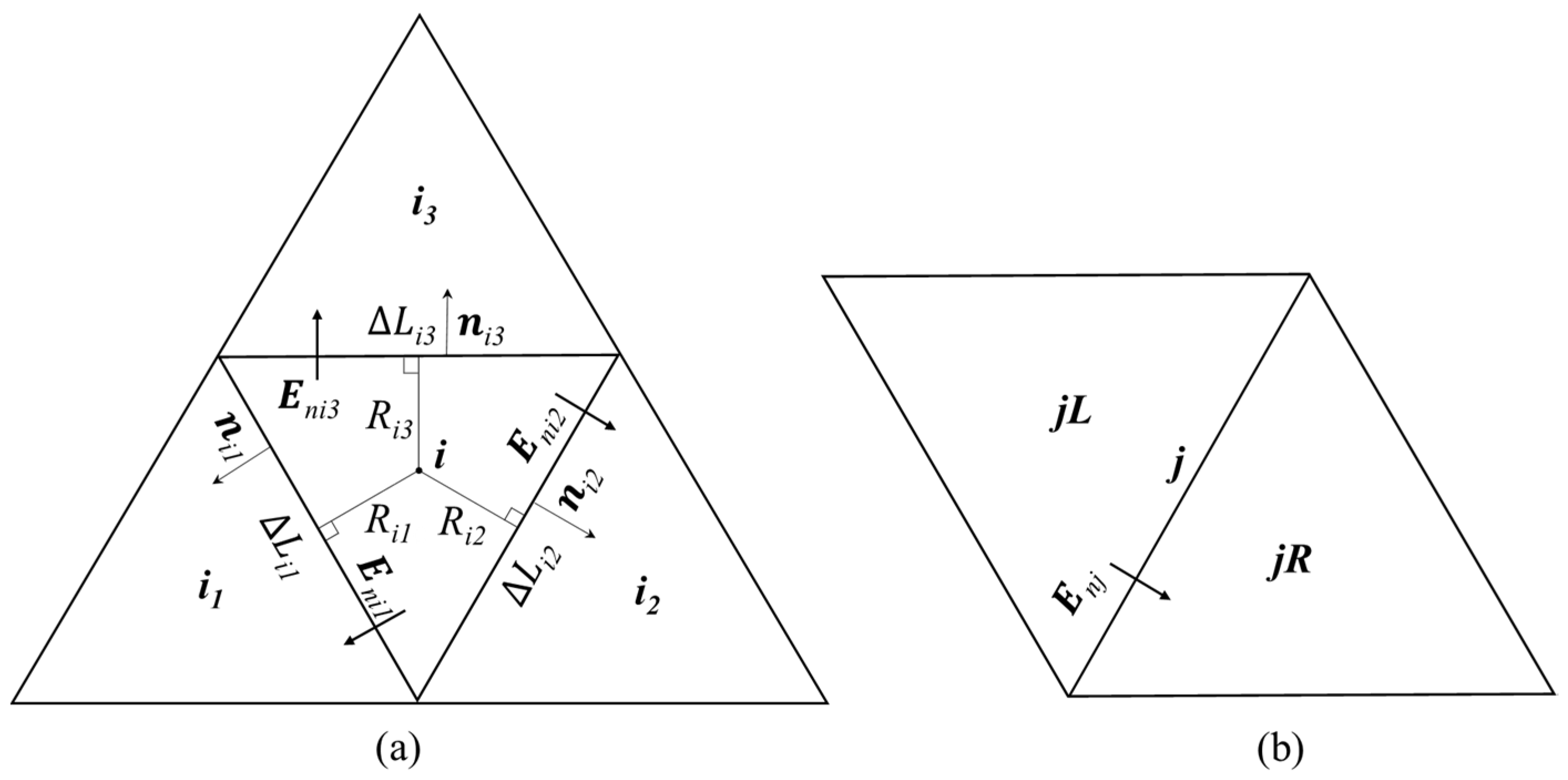
Figure 1 shows a sketch of unstructured triangular meshes: (a) an internal triangular cell (ID: $i$) and its three neighboring cells (ID: $i_1$, $i_2$, $i_3$); (b) a face (ID: $j$) and its neighboring (left and right) cells (ID: $jL$, $jR$). Cell ID varies from 1 to $N_c$; Face ID varies from 1 to $N_f$. Finite volume discretization of Equation (1) on the cell (i) gives.

$$U_i^{**}=U_i^{*}-\frac{\Delta t_i}{A_i}{\displaystyle \sum _{j=1}^3{E}_{nij}\Delta L_{ij}}+\Delta t_i{S}_i,i=1,2,3,~,N_c$$

(3)

where $U_i^{*}$ and $U_i^{**}$ are the conserved physical variables of the cell (i) at the time level $t$ (indicated by superscript ‘*’) and the time level $t+\Delta t_i$ (indicated by superscript ‘**’); $A_i$ is the cell area; $\Delta t_i$ is the time step (see the Section 2.3); $E_{nij}={\left(F{n}_x+G{n}_y\right)}_{ij}$ is the numerical flux across the jth-face of the cell (i), where j = 1, 2, 3; $n_{ij}={\left(n_x,n_y\right)}_{ij}$ are the normal outward direction of the jth-face of the cell (i); $\Delta L_{ij}$ is the jth-face length of the cell (i); and $S_i$ is the cell-averaged source term. The bed slope terms are evaluated using the slope flux method [25]. The bed friction terms are estimated using the splitting point-implicit method [26]. For numerical fluxes at internal faces, the HLLC (Harten-Lax-van Leer-Contact) approximate Riemann solver is adopted. Before calling the subroutine function of the HLLC solver, the left and right Riemann variables are modified using the non-negative water depth reconstruction method [14,15,27,28]. Details of the HLLC solver can be seen in [29]. For numerical fluxes at external faces that coincide with the boundary of the computational domain, they are estimated by the definition using boundary values (water depth, flow velocity) of the physical parameters [30]. For a subcritical flow boundary, the boundary values can be solved using the Riemann invariants along with the characteristics and the specified inflow discharge/water level (in relation to Flow Scenario 3). For a wall boundary, the free slip condition is applied.

2.3. The Local Time Step Estimations

This section presents details on how to estimate local time steps. The first step is to compute the locally allowable maximum time step $\Delta t_{ami}$ for cell (i):

$$\Delta t_{ami}=Cr\frac{R_{mi}}{\sqrt{u_i^2+v_i^2}+\sqrt{g{h}_i}} \mathrm{for} \mathrm{cells} \mathrm{with} h_i\ge h_{thr}$$

(4a)

$$\Delta t_{ami}= \mathrm{an} \mathrm{arbitrarily} \mathrm{large} \mathrm{value} [\mathrm{e}.\mathrm{g}., 100(\mathrm{s}) \mathrm{here}] \mathrm{for} \mathrm{cells} \mathrm{with} h_i<h_{thr}$$

(4b)

where $Cr$ is the Courant number, which is set to 0.9; $h_i$, $u_i$, $v_i$ is the water depth and flow velocities of the cell (i); $R_{mi}=\min \left(R_{i1},R_{i2},R_{i3}\right)$ is the minimum distance from the centroid of cell (i) to its three faces; $R_{i1},R_{i2},R_{i3}$ are distances from the centroid of cell (i) to its three faces (see Figure 1a); $h_{thr}$ is a threshold water depth, which is specified as 10⁻⁶ m. The second step is to compute the global minimum value of time step $\Delta t_{\min }$:

$$\Delta t_{\min }=\underset{i = 1,2,~N_c}{\min (\Delta t_{ami})}$$

(5)

The third step is to compute the ‘potential grade exponent’ $m_i$ for all cells:

$$m_i=\mathrm{int} [\frac{\lg (\Delta t_{ami}/\Delta t_{\min })}{\lg (2)}] \mathrm{with} i=1,2,3,~,N_c$$

(6)

The fourth step is to constrain the potential grade exponent of cells around dynamic/static front [14]. The potential grade exponents of the first- and second-layer cells around a dynamic/static front are modified to the locally minimum value. The fifth step is to compute the grade exponent $m_{fj}$ for faces

$$m_{fj}=\min (m_{jL},m_{jR}) \mathrm{with} j=1,2,3,~,N_f$$

(7)

where the symbols $m_{jL}$ and $m_{jR}$ represent the potential grade exponents of the two neighboring cells around the face (j), see Figure 1b. The sixth step is to compute the actual grade exponent $m_i^{*}$ for cells

$$m_i^{*}=\min (m_i,m_{i1},m_{i2},m_{i3}) \mathrm{with} i=1,2,3,~,N_c$$

(8)

where the symbols $m_{i1},m_{i2},m_{i3}$ indicate the potential grade exponents of the three neighboring cells of the cell (i), see Figure 1a. Finally, one has to find the maximum value $m_{\max }$ of the actual grade exponents

$$m_{\max }=\underset{i=1,2,~N_c}{\max (m_i^{*})}$$

(9)

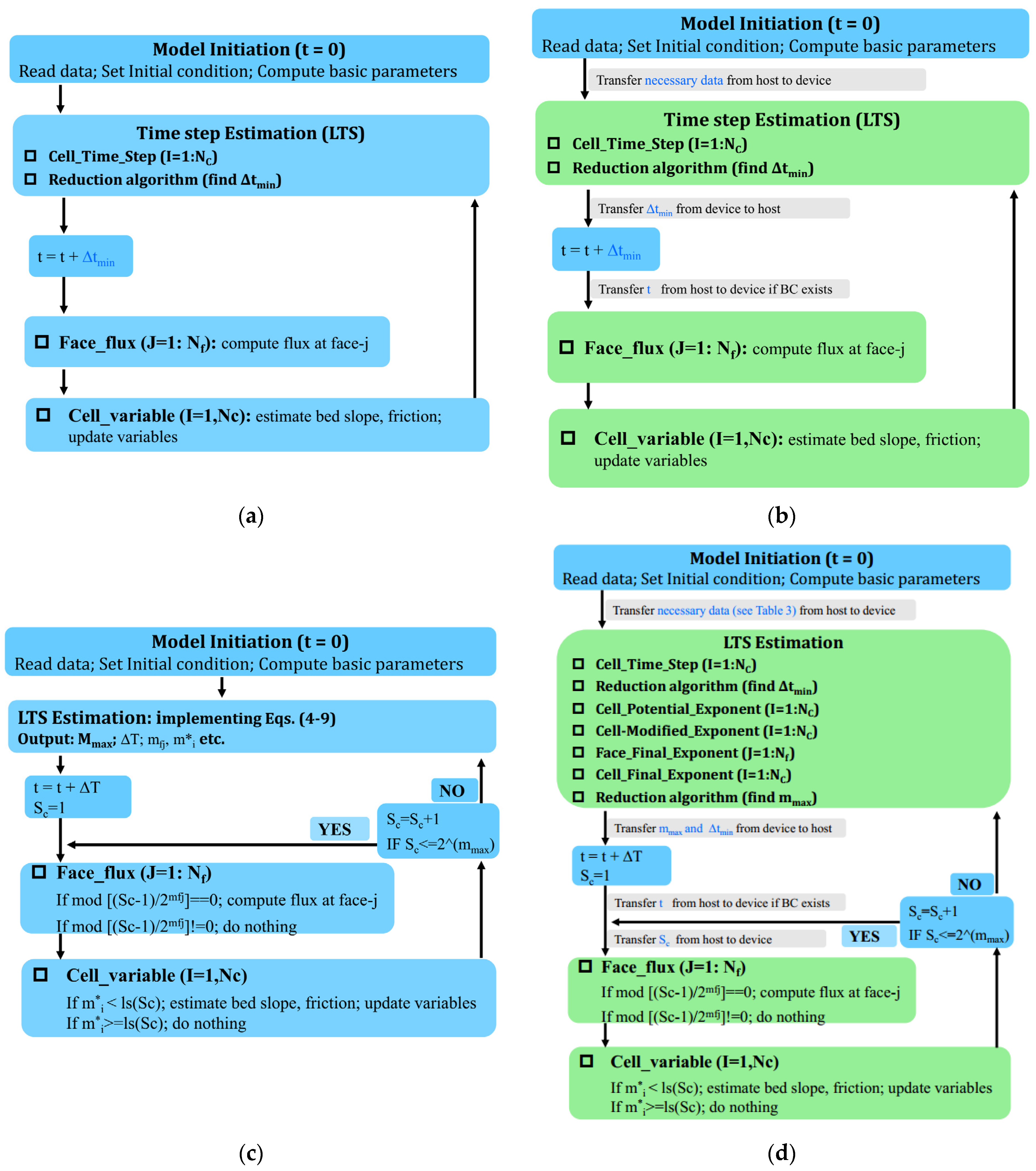
2.4. The Six SWM Versions and Their Numerical Structures

Table 1. Summary of the six SWM versions.

SWM Version		LTS	Parallel Language
V1	single-core CPU	No	NA
V2	(multi-core CPU)		Open MP
V3	GPU		CUDA Fortran
V4	single-core CPU + LTS	YES	NA
V5	multi-core CPU + LTS		Open MP
V6	GPU + LTS		CUDA Fortran

gives a summary of the six SWM versions. Figure 2 presents their numerical structures: (a) Versions 1–2 (single-core/multi-core CPU versions); (b) Version 3 (the GPU version); (c) Versions 4–5 (The LTS versions on CPU: single-core/multi-core); (d) Version 6 (the GPU + LTS version). The numerical structures of the Versions 1 and 2 are the same, and those of Versions 4 and 5 are the same. For Versions 1–3 that uses the GMiTS, the time step $\Delta t_i$ in Equation (3) is set equal to $\Delta t_{\min }$ for all cells. This leads to a very simple and straightforward numerical structure (Figure 2a,c): firstly, compute $\Delta t_{\min }$; secondly, compute numerical flux for all faces; thirdly, estimate the bed slope and friction slope source terms and update the flow variables for all cells. For Versions 4–6 that uses LTS (Figure 2b,d): time levels of flow variables are at the same synchronized time every interval of $\Delta T$, where $\Delta T=2^{m_{\max }}\Delta t_{\min }$. Updating from a synchronized time (e.g., $t$) to the next synchronized time (e.g., $t+\Delta T$) is defined as a full cycle, which has $2^{m_{\max }}$ sub-cycles with $S_c=1,2,~,2^{m_{\max }}$. Each sub-cycle has two steps: flux estimation and variable updating. In sub-cycles, whether or not the numerical flux of a specific face needs to be estimated depends on the property of the ratio $(S_c-1)/2^{m_{fj}}$. If this ratio is an integer, the numerical flux of face-j at the $S_c$-th sub-cycle will be refreshed. Whether or not the flow variables of a specific cell need to be updated depends on the inequality $m_i^{*}<l_0(S_c)$. If this inequality is satisfied, flow variables of cell-i at the $S_c$-th will be updated. The function $l_0(S_c)$ can be seen in [14]. Versions 3 and 6 differ from other versions in that GPU acceleration is implemented (Figure 2b vs. Figure 2a; Figure 2d vs. Figure 2c). In Figure 2a–d: blue box means CPU host tasks, yellow box means GPU device tasks (Figure 2b,d), and grey box means data transfer between host and device (Figure 2b,d). The GPU parallel computing on the device is initiated when the host invokes a kernel. For the present model, the total number of threads for a kernel would be $N_c$ or $N_f$, depending on whether cell or edge variables are dealt with. Numerical experiments indicate that when threadsPerBlock ranges from 32 to 512 (i.e., 32, 64, 96, 128, 256, 512), comparable numerical efficiency can be obtained. In particular, when threadsPerBlock is 256, the performance is best; therefore, threadsPerBlock is set to 256 in this paper. The parameter threadsPerBlock is calculated by $N_c$/threadsPerBlock or $N_f$/threadsPerBlock. Moreover, one has to decide which memory type is used for variable storage. Here three types of GPU memory are involved: global memory, constant memory, and texture memory. Variables and big vectors that vary with time are stored in global memory on the device; some of these variables/vectors may be transferred regularly from the device to the host. Variables that do not vary with time are stored in the constant memory on the device. Big vectors that do not vary with time (mostly vectors about mesh information) are stored in texture memory. The present models adopted double precision because of the need to deal with complex topography, wet/dry fronts. The communication between the host and the device is very slow; therefore, data transfer must be minimized, otherwise, the overhead caused by data transfers exceeds the benefits of GPU acceleration. From Figure 2b,d, the data transfer has been kept to a minimum. The following gives a detailed explanation of the numerical structure of the GPU + LTS version.

(a)

The model is initiated on the host by reading data (e.g., mesh information; basic parameters; boundary conditions such as time series of water level or discharge, if any); setting initial conditions; computing basic parameters (e.g., face length, normal direction, cell area). Afterwards, necessary data are transferred from the host (CPU) to the device (GPU). This data transfer occurs once per numerical case, of which the overhead is negligible as compared to the whole computational cost.

(b)

The LTS estimation involves twice implementation of the reduction algorithm (RA1, RA2) and five kernels: Kernel ‘Cell_Time_Step (CTS)’ computes the locally allowable maximum time step; the reduction algorithm (RA1) finds the globally minimum time step; Kernel ‘Cell_Potential_Exponent (CPE)’ computes the potential grade exponent. Kernel ‘Cell-Modified_Exponent (CME)’ modifies the potential grade exponents around dynamic/static fronts. Kernel ‘Face_Final_Exponent (FFE)’ computes the grade exponent of each face. Kernel ‘Cell_Final_Exponent (CFE)’ computes the actual grade exponent of cells. The reduction algorithm (RA2) finds $m_{\max }$.

(c)

The parameter $m_{\max }$ and $\Delta t_{\min }$ is transferred from the device to the host, such that a full cycle of $S_c=1,2,~,2^{m_{\max }}$ can be defined in the host. For each sub-cycle, the parameter $S_c$ is firstly transferred from the host to the device (on constant memory); afterwards, two kernels [Face_Flux (FF), Cell_Variable (CV)] are invoked: ‘Face_Flux (FF)’ computes numerical fluxes of faces; Cell_Variable (CV)’ updates the conserved variables of cells at a time interval of $2^{m_i^{*}}\Delta t_{\min }$ by firstly estimating the bed slope and frictions, and secondly implement Equation (3). At the end of each sub-cycle, $S_c$ is increased by unity until it exceeds $2^{m_{\max }}$, and subsequently, the computation goes to the LTS estimation again.

3. Results and Discussion

In this section, simulations of three flow scenarios are presented: an idealized scenario of dam-break flows; an experimental scenario of partial dam-break flow; a field-scale scenario of tidal flows. These three scenarios cover a wide range of flow conditions: from idealized flow, experimental flow to field flow, from small-scale flow to large-scale flow, from challenging dam-break flow to general river-tidal flow interactions. Each scenario is simulated by the six SWM versions on several sets of meshes. The non-uniformity of the meshes is quantified by statistics of the equivalent face length, which is computed for each cell as the square root of the cell area. The resultant statistics include the following parameters: the mean equivalent face length $L_{50}$, the gradient coefficient $Gc=0.5(L_{84.1}/L_{50}+L_{50}/L_{15.9})$, and the geometric standard deviation $\sigma =\sqrt{L_{84.1}/L_{15.9}}$, where $L_{50}$, $L_{84.1}$, and $L_{15.9}$ are 50%, 84.1%, and 15.9% shorter face lengths, respectively. The computational efficiency of the six SWM versions is evaluated by the parameter of speeding-up ratio, which is defined as the ratio of the computational cost of V1-V6 to that of V1 on different meshes. The lesser the computational cost, the higher the speeding-up ratio is, and thus the higher the computational efficiency. By definition, the speeding-up ratio for V1 is unity (see

Table 2. Statistics for simulations of the idealized dam-break flows (V1-V6 refers to the six SWM versions).

No.	${\mathit{N}}_{\mathit{c}}$$/{\mathit{L}}_{50}$$\left(\mathbf{m}\right)/\mathit{\sigma }$$/\mathit{G}\mathit{c}$	Computational Cost (s) of V1	Speeding-Up Ratios Compared to Single-Core CPU Version						LTS Benefits
			V1	V2	V3	V4	V5	V6	V4 vs. V1	V5 vs. V2	V6 vs. V3
1	1010/0.14/0.7/1.1	0.079	1	1.4	2.6	2.6	2.0	2.3	2.6	1.4	0.9
2	4762/0.066/0.7/1.0	0.585	1	2.4	12.4	2.1	3.8	9.3	2.1	1.6	0.7
3	18,824/0.033/0.7/1.0	6.772	1	2.9	37.4	2.8	6.6	37.2	2.8	2.3	1.0
4	73,508/0.016/0.7/1.0	44.56	1	2.8	77.4	2.2	5.2	82.1	2.2	1.9	1.1

,

Table 3. Statistics for simulations of the scenario of dam-break flow propagating through blocks.

No.	${\mathit{N}}_{\mathit{c}}$$/{\mathit{L}}_{50}$$\left(\mathbf{m}\right)/\mathit{\sigma }$$/\mathit{G}\mathit{c}$	Computational Cost (s) of V1	Speeding-Up Ratios Compared to Single-Core CPU Version						LTS Benefits
			V1	V2	V3	V4	V5	V6	V4 vs. V1	V5 vs. V2	V6 vs. V3
1	5000/0.1/1.5/1.5	2.9	1	1.2	3.7	2.4	3.7	7.3	2.4	3.0	2.0
2	10,510/0.1/1.6/1.7	6.3	1	1.4	6.3	2.1	3.2	7.9	2.1	2.3	1.3
3	20,523/0.07/1.8/2.0	26.3	1	1.9	13.8	3.8	2.3	10.1	3.8	3.4	1.4
4	28,694/0.07/1.7/1.9	72.1	1	2.1	17.6	4.5	8.8	28.8	4.5	4.1	1.6
5	43,302/0.05/1.6/1.8	105.8	1	2.2	25.2	4.5	9.2	39.2	4.5	4.1	1.6
6	68,892/0.04/1.3/1.3	196.0	1	2.1	31.3	3.4	8.0	53.0	3.4	3.8	1.7
7	153,218/0.03/1.4/1.5	694.1	1	2.0	39.4	3.3	7.9	79.8	3.3	4.0	2.0
8	263,115/0.02/1.8/2.1	1628.1	1	1.8	44.2	4.0	8.4	101.8	4.0	4.6	2.3
9	609,916/0.01/1.4/1.5	5954.3	1	1.9	51	3.6	9.1	132.9	3.6	4.9	2.6

and

Table 4. Statistics for simulations of the field-scale scenario of tidal flows in Yangtze Estuary.

No.	${\mathit{N}}_{\mathit{c}}$$/{\mathit{L}}_{50}$$\left(\mathbf{m}\right)/\mathit{\sigma }$$/\mathit{G}\mathit{c}$	Computational Cost (min) of V1	Speeding-Up Ratios Compared to Single-Core CPU Version						LTS Benefits
			V1	V2	V3	V4	V5	V6	V4 vs. V1	V5 vs. V2	V6 vs. V3
1	21,629/10.3/1.7/1.7	20.3	1	3.2	7.0	8.1	33.8	25.4	8.1	10.5	3.6
2	44,606/9.6/1.9/1.9	28.5	1	2.4	10.2	5.6	20.4	35.6	5.6	8.4	3.5
3	61,315/9.6/1.9/2.0	35.7	1	2.9	17.9	6.0	14.3	44.6	6.0	5.0	2.5
4	82,717/9.6/1.8/1.8	59.3	1	2.9	22.0	4.1	12.6	65.9	4.1	4.4	3.0
5	190,308/2.5/1.7/1.8	104.8	1	2.8	18.7	4.1	11.9	61.6	4.1	4.3	3.3
6	269,945/2.4/1.4/1.4	442.9	1	3.1	24.2	6.4	18.1	79.1	6.4	5.9	3.3
7	422,853/1.8/1.2/1.2	662.7	1	3.0	24.6	5.5	18.3	98.9	5.5	6.1	4.0
8	518,175/1.6/1.2/1.2	1024.8	1	2.5	27.0	6.0	19.9	150.7	6.0	8.1	5.6
9	1,756,679/1.3/1.4/1.4	5954.8	1	2.6	108.1	3.5	12.4	350.3	3.5	4.7	3.2

). Moreover, the LTS benefits in terms of the computational efficiency are computed separately for different parallel computing conditions: the ratio of the computational cost of V4 to that of V1 (Both V1 and V4 are based on the single-core CPU computing); the ratio of the computational cost of V5 to that of V2 (both V2 and V5 are based on the multi-core CPU computing); the ratio of the computational cost of V6 to that of V3 (both V3 and V6 are based on GPU acceleration). Comparisons of numerical solutions from different SWE on the same mesh indicate the following understandings. First, parallel computing (both multi-core CPU and GPU) does not affect the quantitative accuracies. Second, numerical discrepancies from the implementation of the LTS are negligible; therefore, inter-comparisons of numerical solutions between different model versions are not presented. The programming language is Intel Fortran for CPU (Intel Skylake Gold 6132) CUDA Fortran for GPU (Tesla k80).

3.1. Simulation of the Idealized Dam-Break Flows

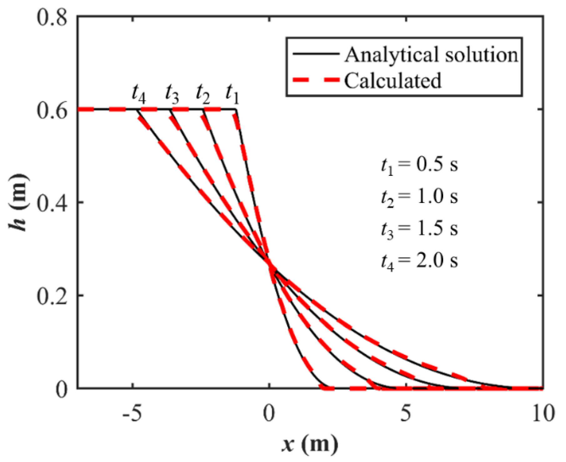
The first flow scenario is the classical idealized dam-break flow over a frictionless and initially dry bed, for which the analytical solution of the flow depth is as follows

$$h(x,t)=\{\begin{array}{ll}{h}_l& x\le x_A\left(t\right)\\ \frac{4}{9g}{\left(\sqrt{g{h}_l}-\frac{x-x_0}{2t}\right)}^2& x_A\left(t\right)\le x\le x_B\left(t\right)\\ 0& x_B\left(t\right)\le x\end{array}$$

(10)

where $h_l$ is the initial water depth behind the dam locating at $x_0=0$; $x_A(t)=x_0-t\sqrt{g{h}_l}$, $x_B(t)=x_0+2t\sqrt{g{h}_l}$. Here a water depth of $h_l=0.6 m$ is used. The six SWM versions are applied to simulate the collapse and propagation of this dam-break flow. The computational domain is set sufficiently large (10 m long and 1 m wide) such that the flood bore does not arrive at the boundary within the simulation time. Four sets of meshes are used (see Table 2), and the relative discrepancies between the numerical and analytical solutions are 7.31 × 10⁻² m, 5.24 × 10⁻² m, 3.46 × 10⁻² m, and 2.30× 10⁻² m for the four set of meshes, respectively. Such magnitudes of quantitative discrepancies are negligible. Figure 3 presents visual comparisons of the computed and analytical solutions for water depth profiles at four transients. From Figure 3, when the water is released, a forward-propagating water bore, and a backward-propagating rarefaction wave are formed.

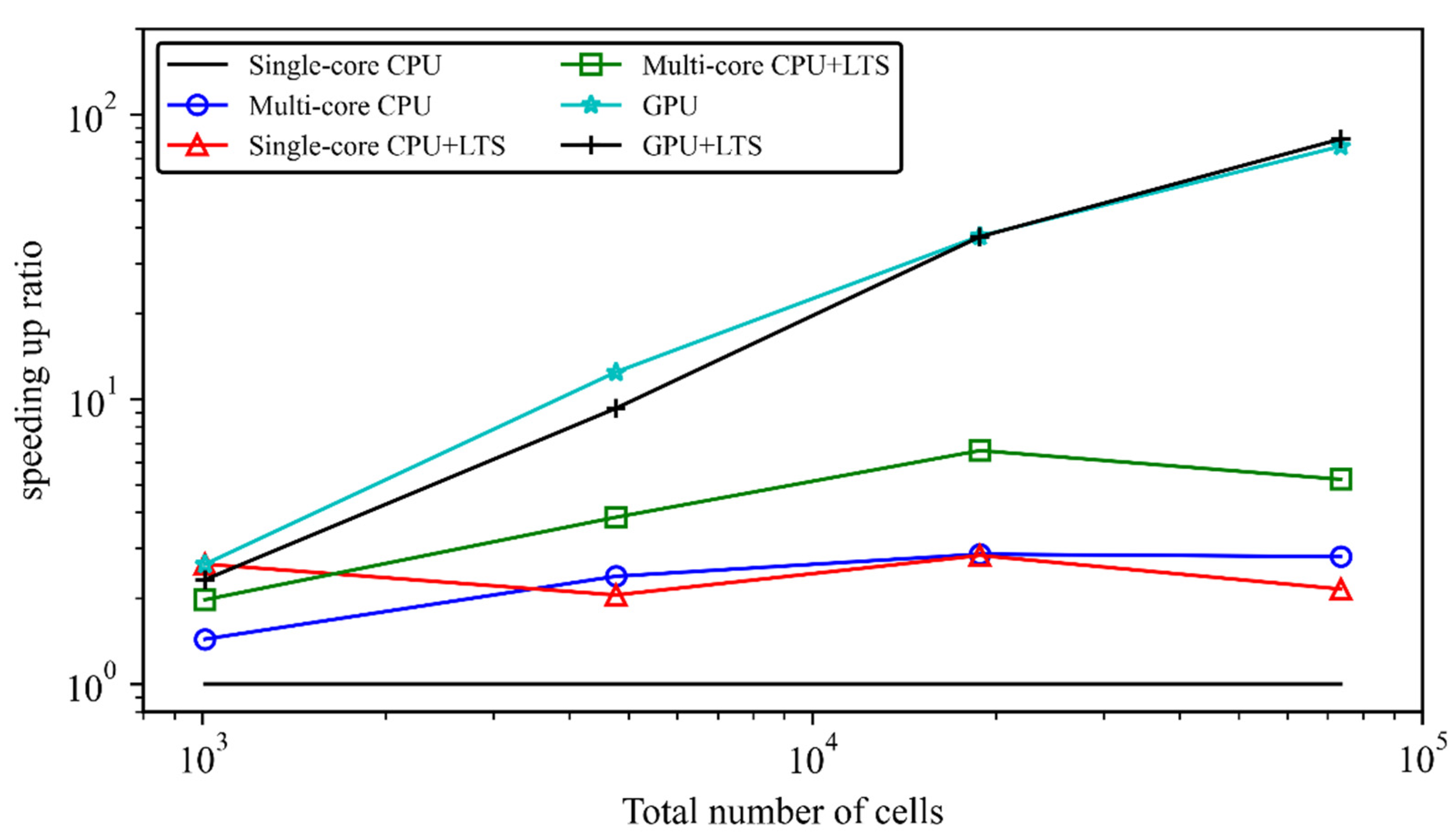
Table 2 gives the mesh information (total number of cells, the mean equivalent length, the geometric standard deviation, and the gradient coefficient), computational cost of V1, the speeding-up ratios of V1-V6, and the LTS benefits. Figure 4 presents the variation of the speeding-up ratios for V1-V6 against the total number of cells. From Table 2 and Figure 4, the computational efficiency of the six SWM can be roughly ranked as follows: single-core CPU (V1) < multiple-core CPU (V2) ≈ single-core CPU + LTS (V4) < multiple-core CPU + LTS (V5) < GPU (V3) < or ≈ GPU + LTS (V6). First, the single-core CPU version of SWM is computationally most demanding, whereas the GPU version and the GPU + LTS version are computationally most efficient. Second, V2 and V4 achieve comparable computational efficiency: the speeding-up ratios for V2 are about 1.4–2.8, whereas those for V4 are about 2.1–2.8. The overall extent of improvement for V2 is basically consistent with previous understanding. In contrast, the speeding-up ratios of V4 (i.e., the LTS benefit) appear to be less than the reported improvement in the literature [14]. This is because the four sets of meshes here are characterized by very uniform cell sizes: the gradient coefficient and the geometric standard deviation are nearly unity, see Table 2. Consequently, the LTS benefits in other parallel computing frameworks are also not significant. For example, the improvement of V5 to V2 is about 1.5–1.6; the improvement of V6 to V3 is about 0.7–1.1 (Implementation of LTS results in additional computational cost). Third, the GPU acceleration leads to a significant reduction in the computational cost, of which the effects become increasingly obvious as the total number of cells increases. For simulations on 73 thousand cells, a speeding-up ratio of about 82 is achieved, which is an order of magnitude larger than that on CPU.

3.2. Simulation of the Experimental Partial Dam-Break Flow Propagating through Buildings

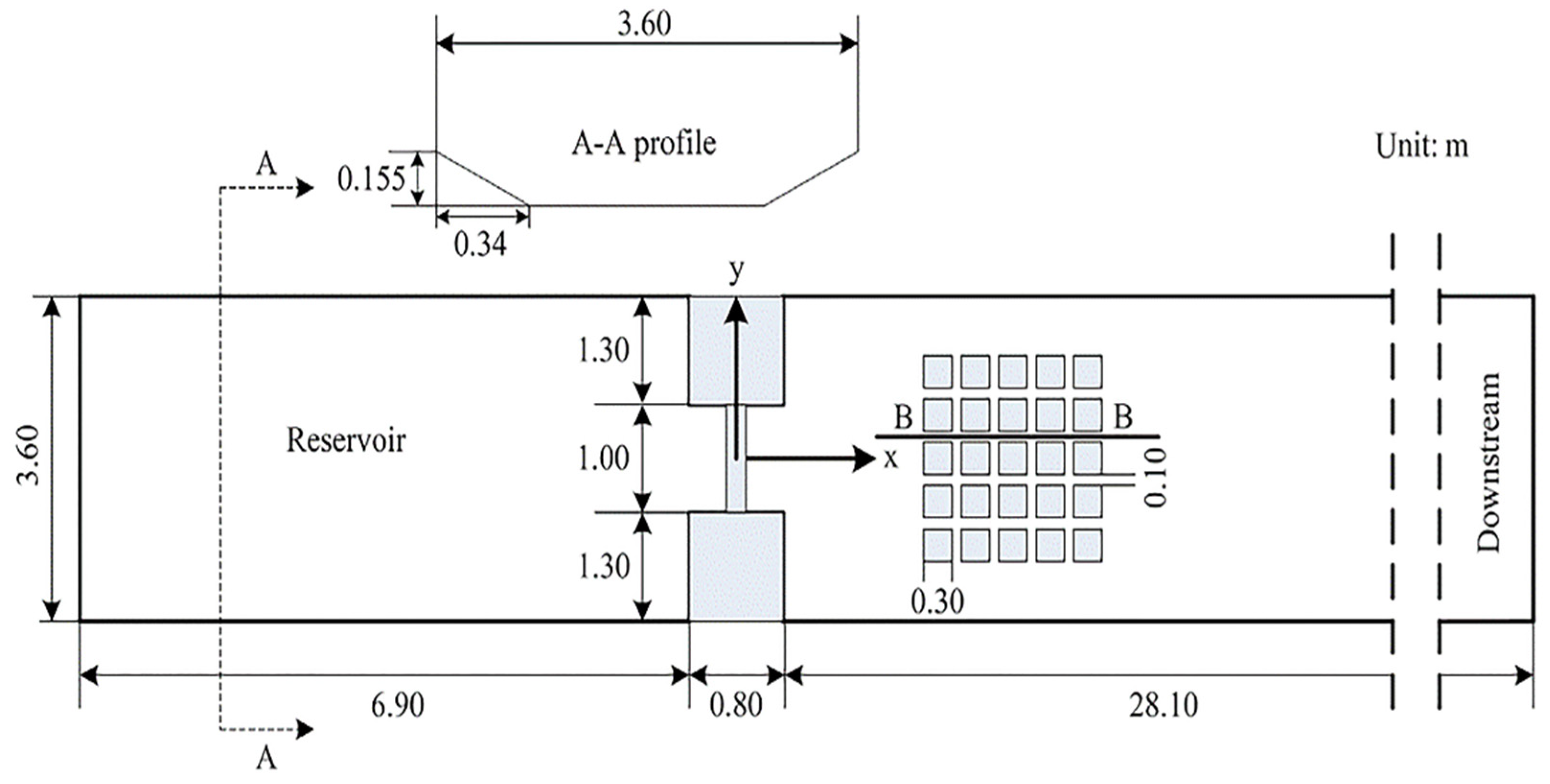
Here, the experimental dam-break flow propagation through buildings [31] is presented. Figure 5 presents a sketch for the experimental flume. The flume is 36 m long and 3.6 m wide, the transverse bed topography is trapezoidal (as the cross-section A-A indicates). Two impervious blocks (1.3 m wide and 0.8 m long for each block) and one wide gate (1 m in width) are arranged at 7.3 m from the left end of the flume. A group of 5 × 5 rigid cubes is placed downstream of the dam; the sides of the cubes are either parallel to or perpendicular to the direction of the main flow; the horizontal dimensions of each cube is 0.3 m × 0.3 m; the distance between two neighboring cubes is 0.1 m (denotes as w1 = 0.1 m). The water depth on the left side is 0.4 m, and that on the right side is 0.011 m. The Manning roughness coefficient is 0.01. Lifting the gate rapidly generates partial dam-break flow.

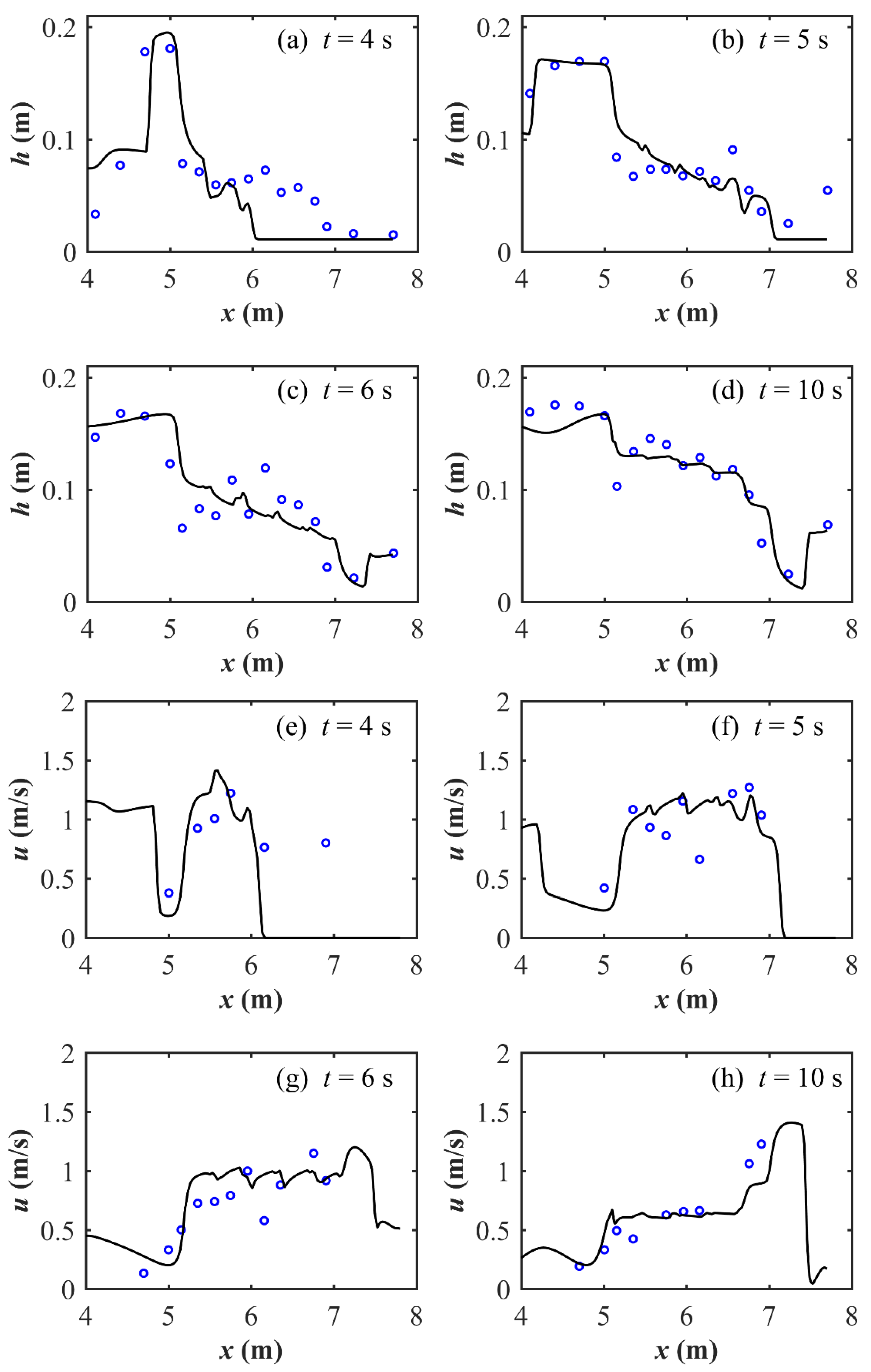
Figure 6 presents the comparison of the computed and measured water depth and flow velocity profiles along the B-B cross-section at several transients. Although the maximum relative discrepancies between the simulated and measured data are about 0.01–0.0385 m for water level and 0.3–0.4 m/s for water velocity, the magnitudes of the simulated water level and velocity are comparable to the measured data. The rigid cubes act to hamper the dam-break flow, leading to a high-water level and low flow velocity at the earlier instants. Afterwards, the hampered water gradually goes through the rigid cube zone, and the water level in the region tends to be uniform as time increases.

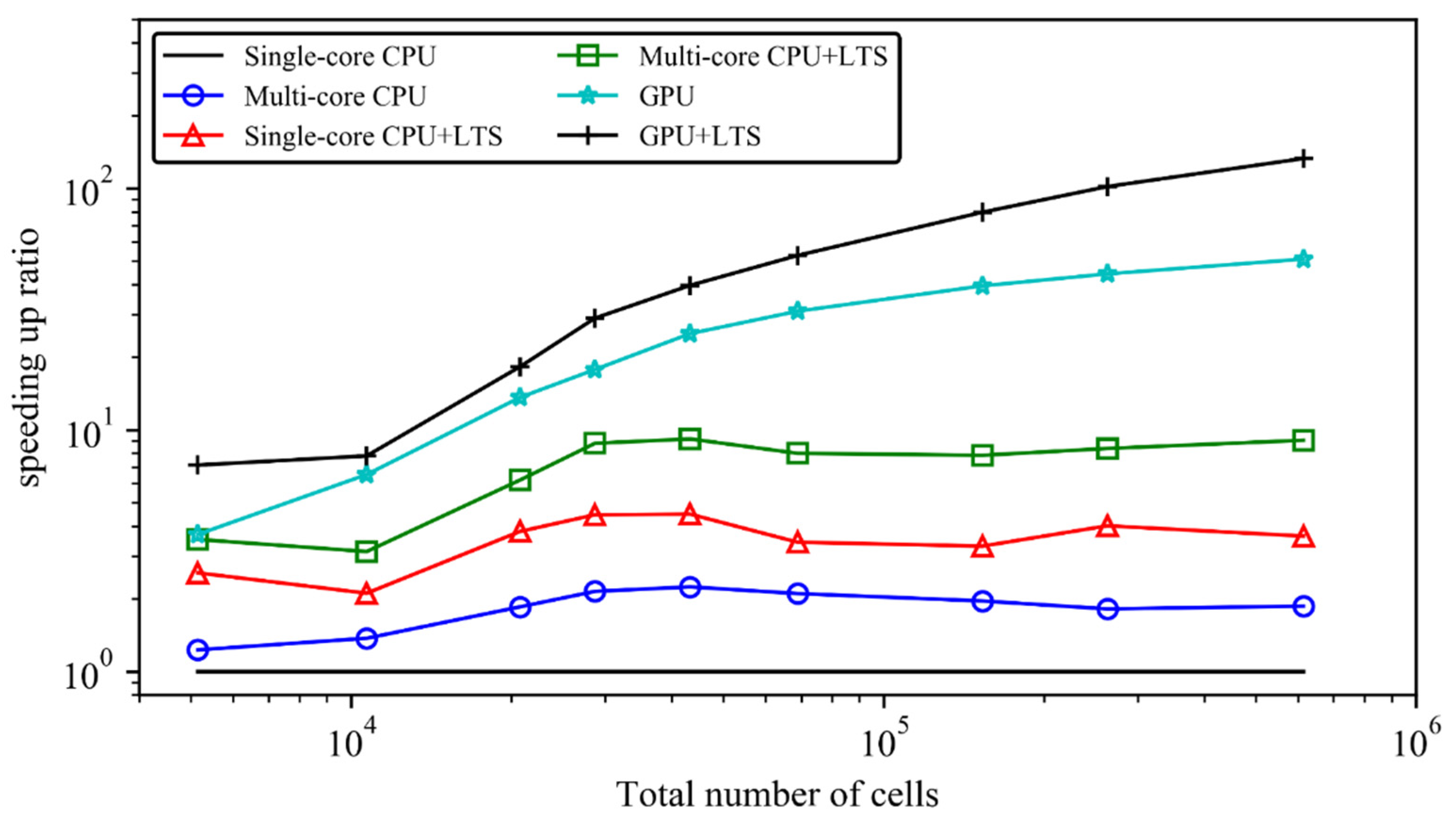
To compare the computational efficiency of different models on different meshes, nine sets of meshes are used, with the total number of cells ranging from 5000 to 609,916. Table 3 summarizes the statistics (total number of cells, the mean equivalent face length, the geometric standard deviation; the gradient coefficient) of the nine sets of meshes, the computational cost of the V1, the speeding-up ratios of the six SWM versions, as well as the LTS benefits. Figure 7 illustrates the speeding-up ratio against the number of cells for the six SWM versions. From Table 3 and Figure 7, the computational efficiency of the six SWM can be ranked as follows: single-core CPU (V1) < multiple-core CPU (V2) < single-core CPU + LTS (V4) < multiple-core CPU + LTS (V5) < GPU (V3) < GPU + LTS (V6). This ordering is slightly different from the first scenario (Section 3.1) in that, here, the computational efficiency of V4 (speeding-up ratios: 2.1–4.5) is appreciably higher than that of V2 (speeding-up ratios: 1.2–2.2). It is because the cell size distributions for this scenario are very non-uniform. Specifically, from Table 3, the geometric standard deviation and the gradient coefficients are about 1.3–1.8 and 1.3–2.1, respectively. Accordingly, the LTS benefits in other parallel computing frameworks are also considerable: the ratio of the computational cost of V5 to that of V2 is about 2.3–4.5 (V2 and V5 are based on the multi-core CPU computing); the ratio of the computational cost of V6 to that of V3 is about 1.3–2.6 (V3 and V6 are based on GPU acceleration). The improvement of the GPU acceleration is similar to that of the first scenario: the effects become increasingly obvious as the total number of cells increases. For simulations on about 610 thousand cells, a speeding-up ratio of about 51 is achieved.

3.3. Simulation of Tidal Flows in Yangtze Estuary and Hangzhou Bay

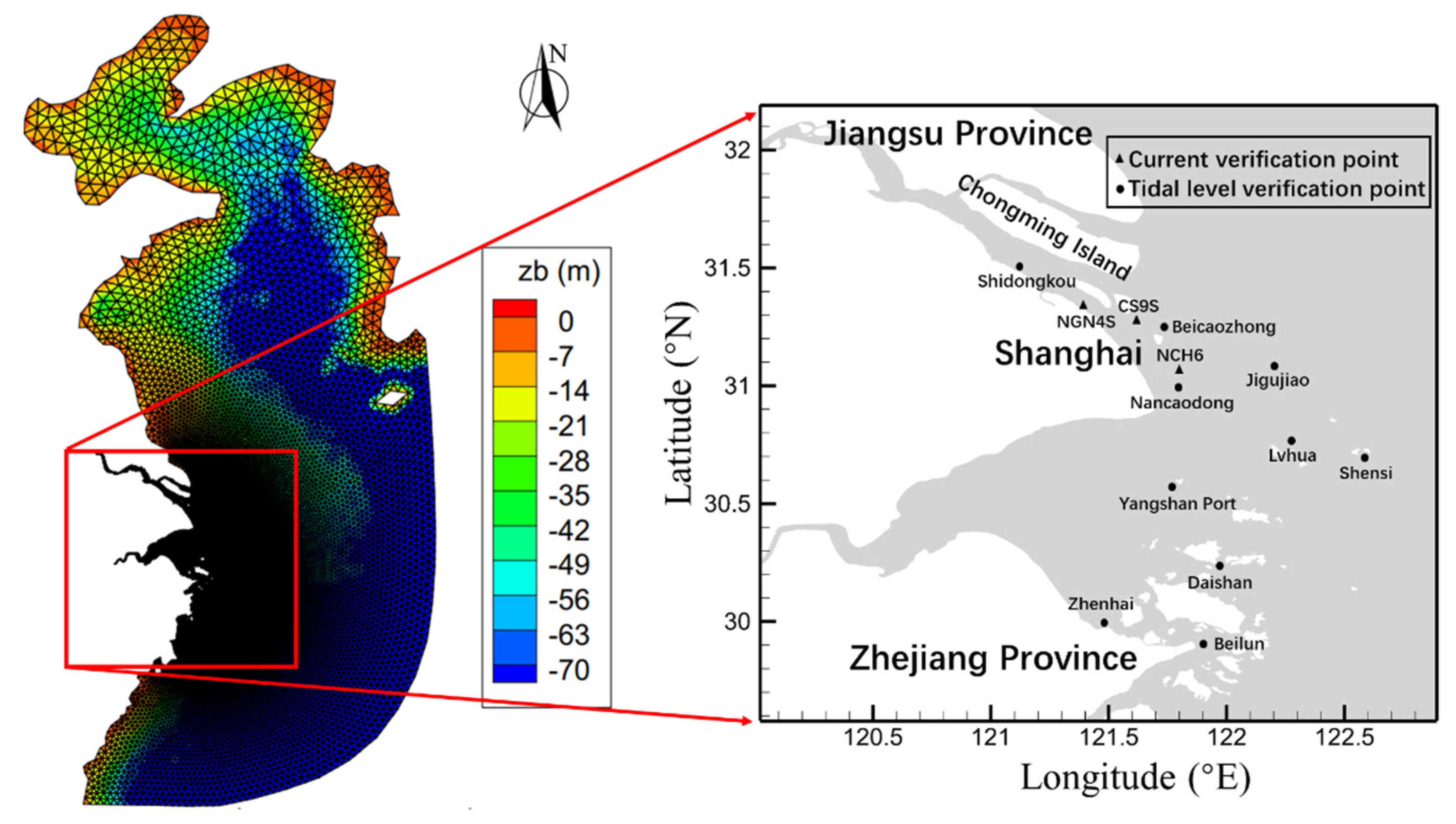
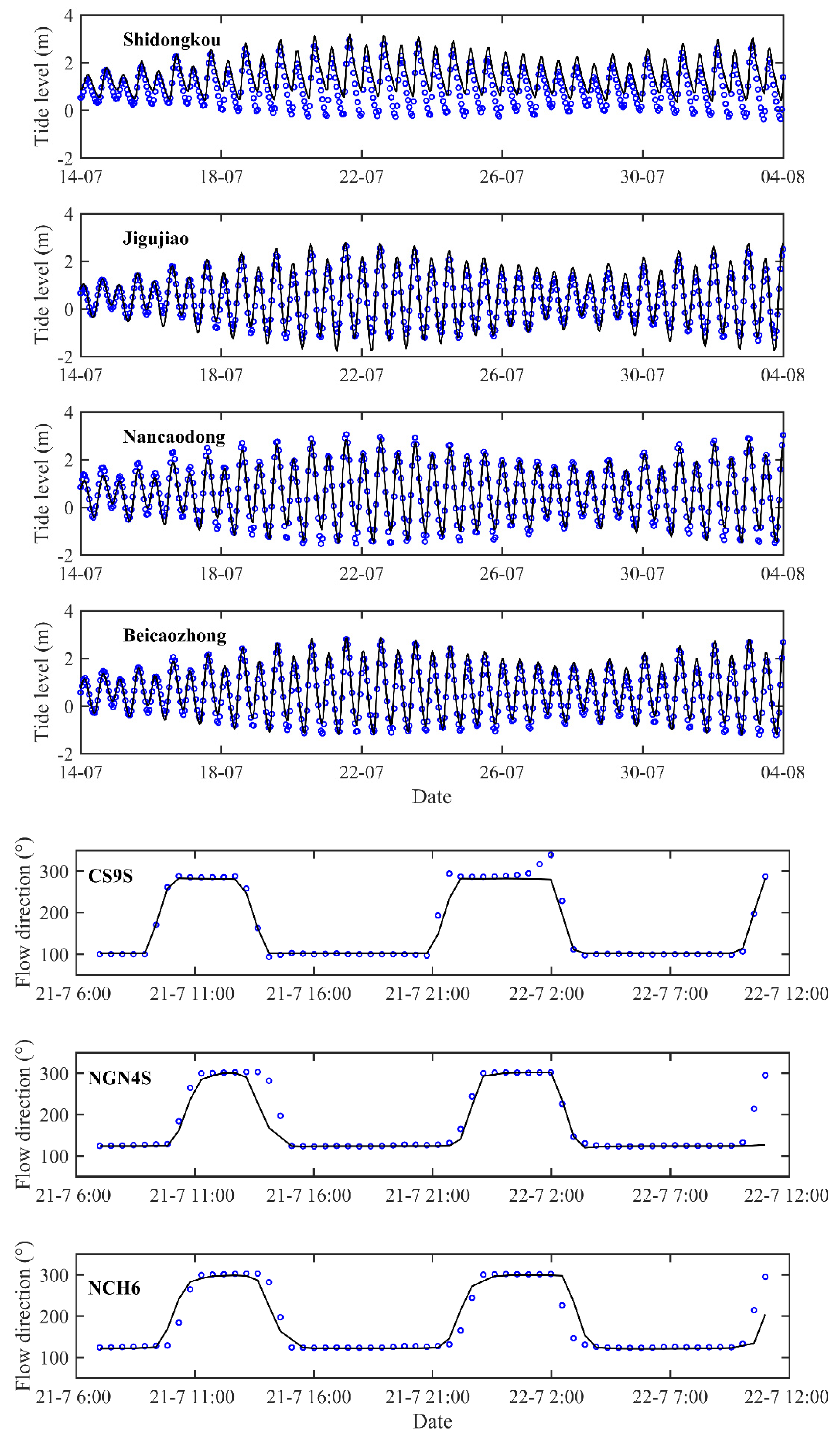
Tidal flows in the Yangtze estuary and Hangzhou bay are presented in this section. Figure 8 presents a set of numerical mesh for the computational domain as well as the embedded bed topography. The computational domain covers the whole East China Sea, Yellow Sea, and Bohai Sea. The computational domain has three open boundaries, including the boundary of the Yangtze River at the Sanjiangying, the boundary of the Qiantang River at the Qiantang River Bridge, and the seaward boundary, which is located on the inner side of the continental shelf. At the Sanjiangying, the measured flow rate is given. At the upstream boundary of the Qiantang River, a constant flow discharge of 800 m³/s is specified. The open sea boundary was driven by nine tidal constituents (i.e., M2, S2, N2, K2, K1, O1, P1, Q1, and M4), which are obtained from TPXO. The Manning roughness is set equal to 0.01 + 0.012/h. Although strong sediment transport occurs in the Yangtze estuary and the Hangzhou bay, only clear-water flow over a fixed bed was simulated in this paper.

Figure 9 compares the computed and measured water level and velocities at several stations of the Yangtze estuary and Hangzhou bay. From Figure 9, there are some deviations between the simulated tidal velocity and measured data, especially at Shidongkou, NCH6, and CS9S. The reason for this discrepancy may be that the locations of these stations are easily disturbed by the incident flow and reflected flow from the coasts and channel. Overall, the above validation generally shows the present model’s good capability in the reproduction of tidal hydrodynamics. To compare the computational efficiency of different models on different meshes, nine sets of meshes are considered for this flow scenario, with the total number of cells ranging from about 21.6 thousand to as much as about 1.76 million. Table 4 presents the statistics of the mesh information as well as the computational cost, the speeding-up ratios of the six versions of SWMs. Figure 10 gives the speeding-up ratios under different mesh sizes. From Figure 10 and Table 4, the computational efficiency of the six SWM can be roughly ranked as follows: single-core CPU (V1) < multiple-core CPU (V2) < single-core CPU + LTS (V4) < multiple-core CPU + LTS (V5) < (for large amount of cells) or > (for relatively small amount of meshes) GPU (V3) < GPU + LTS (V6). This ordering is again slightly different from the above scenarios. Specifically, the relative computational efficiency of V5 and V3 strongly depends on the number of cells (Table 4; Figure 10). For simulations with 21.6 and 44.6 thousand cells, V5 (multiple-core CPU + LTS) runs faster than V3 (GPU), in contrast to those simulations with more cells. This indicates the strong capability of LTS. If the cell sizes and flow strengths are very non-uniform, the advantage of the LTS benefits may overturn that of GPU acceleration. The improvement of the GPU acceleration is similar to that of the first and second scenarios: the effects become increasingly obvious as the total number of cells increases. For simulations on about 1.75 million cells, a speeding-up ratio exceeding 100 is achieved.

4. Conclusions

In this paper, a novel shallow water model is presented based on the LTS method and GPU parallel computing. The model was compared against five additional versions of shallow water models. For the same set of numerical meshes, negligible differences are ensured for numerical solutions from different versions of SWMs. Comparisons between numerical solutions and the available measured data/analytical solution indicate the quantitative accuracy of the model: hydrodynamics of tidal flows in the Yangtze estuary as well as the challenging dam-break flows are satisfactorily resolved by the present models. Inter-comparisons of the computational efficiency of the six SWM versions indicate the following. First, GPU acceleration is much more efficient than multi-core CPU parallel computing. Specifically, the speed ups of GPU can be as high as a hundred, whereas those for multi-core CPU are only 2–3. Second, implementing the LTS can further bring considerable reduction: the additional maximum speed-ups can be as high as 10 for the single-core CPU/multi-core CPU versions and as high as five for the GPU versions. Third, the GPU + LTS version is computationally most efficient in most cases; the multi-core CPU + LTS version may run as fast as a GPU version for scenarios over some intermediate number of cells. It is worth pointing out that the results are affected by the specific usage of computer hardware. Extension of the present model to sediment transport problems can facilitate physical process-based decadal morphodynamic modeling.

References

- Cea, L.; French, J.R.; Vazquez-Cendon, M.E. Numerical modelling of tidal flows in complex estuaries including turbulence: An unstructured finite volume solver and experimental validation. Int. J. Numer. Methods Eng. 2006, 67, 1909–1932. [Google Scholar] [CrossRef]
- Hu, P.; Han, J.J.; Li, W.; Sun, Z.L.; He, Z.G. Numerical investigation of a sandbar formation and evolution in a tide-dominated estuary using a hydro-sediment-morphodynamic model. Coast. Eng. J. 2018, 60, 466–483. [Google Scholar] [CrossRef]
- Luan, H.L.; Ding, P.X.; Wang, Z.B.; Ge, J.Z. Process-based morphodynamic modeling of the Yangtze Estuary at a decadal timescale: Controls on estuarine evolution and future trends. Geomorphology 2017, 290, 347–364. [Google Scholar] [CrossRef]
- Qin, X.; LeVeque, R.J.; Motley, M.R. Accelerating an adaptive mesh refinement code for depth-averaged flows using GPUs. J. Adv. Modeling Earth Syst. 2019, 11, 2606–2628. [Google Scholar] [CrossRef] [Green Version]
- Kim, D.H.; Cho, Y.S.; Yi, Y.K. Propagation and run-up of nearshore tsunamis with HLLC approximate Riemann solver. Ocean Eng. 2007, 34, 1164–1173. [Google Scholar] [CrossRef]
- Kernkamp, H.W.J.; van Dam, A.; Stelling, G.S.; de Goede, E.D. Efficient scheme for the shallow water equations on unstructured grids with application to the Continental Shelf. Ocean Dyn. 2011, 61, 1175–1188. [Google Scholar] [CrossRef]
- Hu, P.; Li, W.; He, Z.G.; Pahtz, T.; Yue, Z.Y. Well-balanced and flexible modelling of swash hydrodynamics and sediment transport. Coast. Eng. 2015, 96, 27–37. [Google Scholar] [CrossRef] [Green Version]
- Hu, P.; Tan, L.; He, Z. Numerical investigation on the adaptation of dam-break flow-induced bed load transport to the capacity regime over a sloping bed. J. Coast. Res. 2020, 36, 1237–1246. [Google Scholar] [CrossRef]
- Yu, H.; Huang, G.; Wu, C. Efficient finite volume model for shallow-water flows using an Implicit Dual Time-Stepping Method. J. Hydraul. Eng. ASCE 2015, 141, 04015004. [Google Scholar] [CrossRef]
- Gaudreault, S.; Pudykiewicz, J.A. An efficient exponential time integration method for the numerical solution of the shallow water equations on the spher. J. Comput. Phys. 2016, 322, 827–848. [Google Scholar] [CrossRef] [Green Version]
- Crossley, A.J.; Wright, N.G. Time accurate local time stepping for the unsteady shallow water equations. Int. J. Numer. Methods Fluids 2005, 48, 775–799. [Google Scholar] [CrossRef]
- Dazzi, S.; Maranzoni, A.; Mignosa, P. Local time stepping applied to mixed flow modeling. J. Hydraul. Res. 2016, 54, 1–13. [Google Scholar] [CrossRef]
- Dazzi, S.; Vacondio, R.; Palu, A.D.; Mignosa, P. A local time stepping algorithm for GPU-accelerated 2D shallow water models. Adv. Water Resour. 2018, 111, 274–288. [Google Scholar] [CrossRef]
- Hu, P.; Lei, Y.L.; Han, J.J.; Cao, Z.X.; Liu, H.H.; Yue, Z.Y.; He, Z.G. An improved local-time-step for 2D shallow water modeling based on unstructured grids. J. Hydraul. Eng. ASCE 2019, 145, 06019017. [Google Scholar] [CrossRef]
- Hu, P.; Lei, Y.L.; Han, J.J.; Cao, Z.X.; Liu, H.H.; He, Z.G. Computationally efficient hydro-morphodynamic modelling using a hybrid local-time-step and the global maximum-time-step. Adv. Water Resour. 2019, 127, 26–38. [Google Scholar] [CrossRef]
- Sanders, B.F. Integration of a shallow water model with a local time step. J. Hydraul. Res. 2008, 46, 466–475. [Google Scholar] [CrossRef]
- Sanders, B.F.; Schubert, J.E.; Detwiler, R.L. ParBreZo: A parallel, unstructured grid, Godunov-type, shallow-water code for high-resolution flood inundation modeling at the regional scale. Adv. Water Resour. 2010, 33, 1456–1467. [Google Scholar] [CrossRef]
- Sanders, B.F.; Schubert, J.E. PRIMo: Parallel raster inundation model. Adv. Water Resour. 2019, 126, 79–95. [Google Scholar] [CrossRef]
- Brodtkorb, A.R.; Sætra, M.L.; Altinakar, M. Efficient shallow water simulations on GPUs: Implementation, visualization, verification, and validation. Comput. Fluids 2012, 55, 1–12. [Google Scholar] [CrossRef]
- Castro, M.J.; Ortega, S.; de la Asuncion, M.; Mantas, J.M.; Gallardo, J.M. GPU computing for shallow water flow simulation based on finite volume schemes. Comptes Rendus Mécanique 2011, 339, 165–184. [Google Scholar] [CrossRef]
- de la Asuncion, M.; Castro, M.J. Simulation of tsunamis generated by landslides using adaptive mesh refinement on GPU. J. Comput. Phys. 2017, 345, 91–110. [Google Scholar] [CrossRef]
- Lacasta, A.; Morales-Hernandez, M.; Murillo, J.; Garcia-Navarro, P. An optimized GPU implementation of a 2D free surface simulation model on unstructured meshes. Adv. Eng. Softw. 2014, 78, 1–15. [Google Scholar] [CrossRef]
- Lacasta, A.; Morales-Hernandez, M.; Murillo, J.; Garcia-Navarro, P. GPU implementation of the 2D shallow water equations for the simulation of rainfall/runoff events. Environ. Earth Sci. 2015, 74, 7295–7305. [Google Scholar] [CrossRef]
- Vacondio, R.; Palu, A.D.; Ferrari, A.; Mignosa, P.; Aureli, F.; Dazzi, S. A non-uniform efficient grid type for GPU-parallel Shallow Water Equations models. Environ. Model. Softw. 2017, 88, 119–137. [Google Scholar] [CrossRef]
- Hou, J.; Liang, Q.; Simons, F.; Hinkelmann, R. A 2D well-balanced shallow flow model for unstructured grids with novel slope source term treatment. Adv. Water Resour. 2013, 52, 107–131. [Google Scholar] [CrossRef]
- Liang, Q.; Marche, F. Numerical resolution of well-balanced shallow water equations with complex source terms. Adv. Water Resour. 2009, 32, 873–884. [Google Scholar] [CrossRef]
- Audusse, E.; Bouchut, F.; Bristeau, M.; Klein, R.; Perthame, B.T. A fast and stable well-balanced scheme with hydrostatic reconstruction for shallow water flows. SIAM J. Sci. Comput. 2004, 25, 2050–2065. [Google Scholar] [CrossRef]
- He, Z.G.; Wu, T.; Weng, H.X.; Hu, P.; Wu, G.F. Numerical investigation of the vegetation effects on dam-flows and bed morphological changes. Int. J. Sediment Res. 2017, 32, 105–120. [Google Scholar] [CrossRef]
- Toro, E. Shock-Capturing Methods for Free-Surface Shallow Flows; Wiley: Chichester, UK, 2001. [Google Scholar]
- Yoon, T.H.; Kang, S. Finite volume model for two-dimensional shallow water flows on unstructured grids. J. Hydraul. Eng. ASCE 2004, 130, 678–688. [Google Scholar] [CrossRef]
- Soares-Frazão, S.; Zech, Y. Dam-break flow through an idealised city. J. Hydraul. Res. IAHR 2008, 46, 648–658. [Google Scholar] [CrossRef] [Green Version]
Figure 1.
Sketches of the unstructured triangular meshes: (a) an internal cell (i) and its three neighboring cells; (b) a face (j) and its two neighboring cells (jL and jR).
Figure 2.
Numerical structures of these six versions: (a) single-core CPU and multi-core CPU; (b) GPU; (c) single-core CPU + LTS, and multi-core CPU + LTS; (d) GPU + LTS.
Figure 3.
Longitudinal profiles of the computed and analytical water depth at four transients.
Figure 4.
Speeding-up ratios of the six SWM versions for simulations of the dam break flows, as compared to the single-core CPU version.
Figure 5.
Experimental configuration for dam-break flows through idealized city (modified from [28]).
Figure 6.
Computed and measured hydrodynamics: (a–d) water level profiles; (e–h) flow velocity profiles along the B-B section at four transients.
Figure 7.
Speeding-up ratios of the six SWM versions for simulations of the experimental dam-break flows propagating through buildings, as compared to the single-core CPU version.
Figure 8.
Initial bed topography of computational domain, unstructured mesh and stations for Yangtze estuary and Hangzhou bay case.
Figure 9.
Computed and measured tidal dynamics of the Yangtze estuary and Hangzhou bay.
Figure 10.
Speeding-up ratios of the six SWM versions for simulations of tidal flows, as compared to the single-core CPU version.