Scaling an Artificial Neural Network-Based Water Quality Index Model from Small to Large Catchments

Abstract

Scaling models is one of the challenges for water resource planning and management, with the aim of bringing the developed models into practice by applying them to predict water quality and quantity for catchments that lack sufficient data. For this study, we evaluated artificial neural network (ANN) training algorithms to predict the water quality index in a source catchment. Then, multiple linear regression (MLR) models were developed, using the predicted water quality index of the ANN training algorithms and water quality variables, as dependent and independent variables, respectively. The most appropriate MLR model has been selected on the basis of the Akaike information criterion, sensitivity and uncertainty analyses. The performance of the MLR model was then evaluated by a variable aggregation and disaggregation approach, for upscaling and downscaling proposes, using the data from four very large- and three large-sized catchments and from eight medium-, three small- and seven very small-sized catchments, where they are located in the southern basin of the Caspian Sea. The performance of seven artificial neural network training algorithms, including Quick Propagation, Conjugate Gradient Descent, Quasi-Newton, Limited Memory Quasi-Newton, Levenberg–Marquardt, Online Back Propagation, and Batch Back Propagation, has been evaluated to predict the water quality index. The results show that the highest mean absolute error was observed in the WQI, as predicted by the ANN LM training algorithm; the lowest error values were for the ANN LMQN and CGD training algorithms. Our findings also indicate that for upscaling, the aggregated MLR model could provide reliable performance to predict the water quality index, since the r² coefficient of the models varies from 0.73 ± 0.2 for large catchments, to 0.85 ± 0.15 for very large catchments, and for downscaling, the r² coefficient of the disaggregated MLR model ranges from 0.93 ± 0.05 for very large catchments, to 0.97 ± 0.02 for medium catchments. Therefore, scaled models could be applied to catchments that lack sufficient data to perform a rapid assessment of the water quality index in the study area.

1. Introduction

In recent years, the issue of water quality has been raised as one of the main issues in surface water resources [1]. Natural and human processes, such as runoff and nutrient leaching from the soil [2], agricultural practice [3], landscape and land use patterns [4,5], and urban development [6], are among the main factors that affect water quality in hydrological units. However, the classification of water quality is crucial for monitoring, forecasting, managing [7] and protecting water resources [8,9,10]. The complexity of studying hydrological processes has led to the need for scale-based approaches to assess the catchments and understand their processes and problems [11]. The quality of river water has been studied at different scales, ranging from local [12,13,14,15], to regional [16,17] and national [18], using various models. Most studies on the calibration of hydrological models have been based on local parameters. However, the results can be generalized to areas lacking data, provided that the parameters are calibrated on a larger scale [19].

According to Fritsch et al. 2020 [20], scaling is defined as translating information from one scale, which serves as the source, to another scale, the target. Consequently, scaling can be performed in two forms: upscaling and downscaling [21]. Upscaling refers to the aggregation of data from a smaller to a larger scale [22]. It is associated with a decrease in data requirements and a change in the performance of models of interest [23]. Therefore, these models can be used as a tool for policy making on larger scales, such as regional and national scales [24], and if downscaled, they can support local decision making in socio-ecological management. Upscaling can be a straightforward process, but encountering an unknown number of control variables that play their roles at different scales can be considered a crucial issue for any downscaling practice. Accordingly, even though the aggregation of variables and data is not considered a tedious task in the upscaling process, downscaling is associated with the disaggregation of variables and data, which need to be assembled with the source model. The scale at which the source model is developed requires a different number of variables; the lower the scale, the higher the number of control variables. The data-intensive property of a given model is consequently increased as the scale of interest is changed downward, from the global scale to the local one.

Wilby and Wigley (1997) [25], as cited by Karger et al. (2017) [26], classified downscaling methods into four groups: regression methods, pattern-based approaches, stochastic variable generators, and dynamical downscaling methods. The last of these is of the area-specific feature. Of these approaches, regression methods are the most commonly used downscaling models due to their relative simplicity in implementation and low computational requirements [27].

The application of regression models to upscaling practices was discussed by Zirlewagen and Von Wilpert (2010) [28], who noted that regression techniques are still recommended if accurate spatial predictions of environmental parameters are sought in cause-and-effect relationships. Leitao et al. (2018) [29] applied multidimensional satellite imagery as auxiliary data to upscale above-ground carbon. Applying the regression-based method, their findings indicated that data extrapolation can be performed in a suitable way, using linear regression models.

However, changing from one scale to another is not always easy and causes problems due to nonlinear relationships, scale breaks, feedback, and heterogeneity in process patterns [20,30]. Limitations in data access, the time-consuming nature of multiple algorithms, and uncertainty in modeling require the use of local models that can be implemented on multiple scales. Consequently, it is necessary to apply a suitable basic algorithm to simulate catchment processes and patterns, especially in the field of water resource quality on the local scale, to use the simulated models confidently on multiple scales. The main challenge that underlies upscaling is the lack of a well-accepted upscaling procedure to transform processes [31]. Furthermore, the lack of scalability of local models for larger-scale datasets can be considered another crucial challenge [15,32].

It should be noted that most of the measured data related to nonpoint source pollution, originating from observations and experiments on a laboratory and/or field scale, which helps to understand the processes under which the nonpoint source pollution occurs in the environment. However, simulating nonpoint source pollution on the catchment scale, using laboratory data, is associated with additional model uncertainty, as it cannot accurately reflect nonpoint source pollution patterns on a larger scale [22]. Relationships between macronutrients are also highly scale dependent [33], and increasing the scale of field observations can provide better input data to model catchment nutrients [34,35]. However, Mineau et al. (2015) [36] showed that upscaling field-scale processes are needed to understand the impact of agricultural nonpoint source pollution on receiving lakes.

Many studies have shown the applicability of artificial neural networks (ANN) in the prediction of water quality [12,37,38], suspended sediment concentration [39], water quality monitoring [40], and water quality index [41], as a tool for modeling complex nonlinear systems. ANN training algorithms have been widely used by scientists to solve engineering problems in water quality [42,43,44], hydrological and hydraulic modeling of the catchment [45,46]. Applying ANN models (see, e.g., [47,48]) to predict water quality indices [10,49] has also shown that they can be considered an appropriate model to predict water quality indices.

It should be noted that applying ANN models on another scale requires determining the linear relationships of the model, with little data to achieve the most optimal performance. The group of models that are developed and presently used to predict water quality are always highly data intensive in their training/calibrating stage, time consuming in information processing, and they also require sufficient user knowledge to perform them. Furthermore, considering the factors that affect water quality and their rapid temporal and spatial changes, there is a crucial need for models that could support the formulation of strategies and policies with minimal data and time requirements. To fill the gap, the present study was conducted to assess how well the ANN training algorithms predict water quality indices, if they are up- and downscaled, using MLR models.

2. Materials and Methods

2.1. Study Area

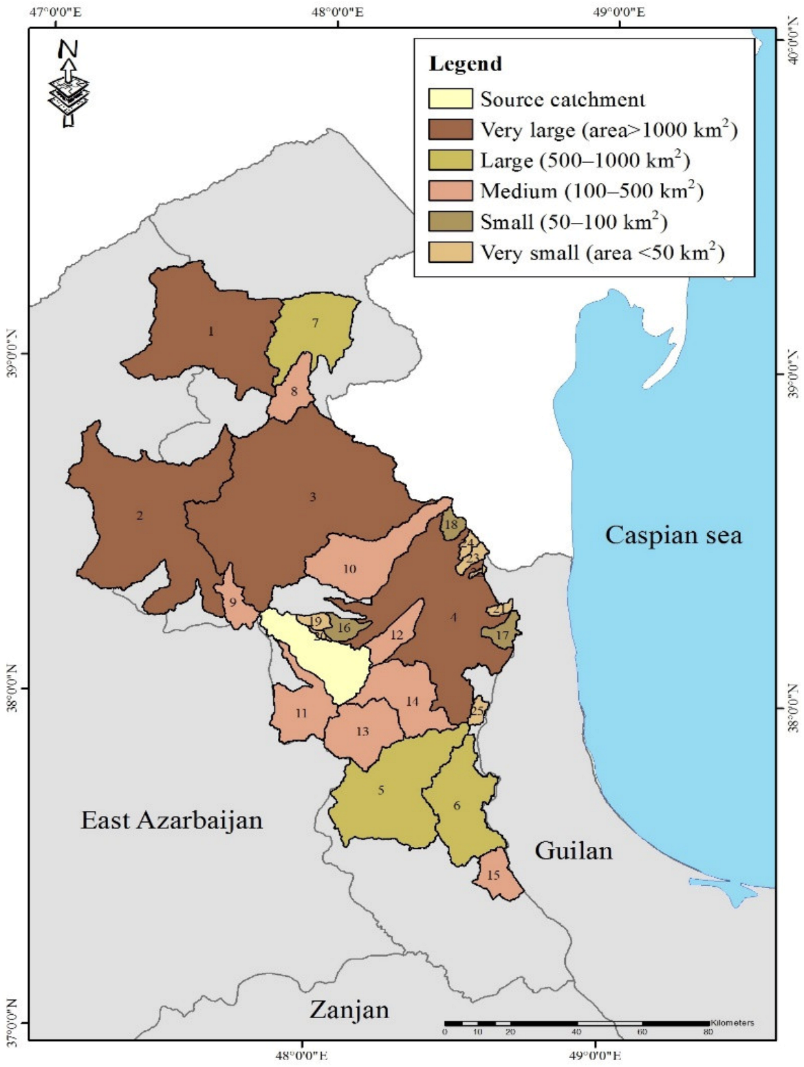
A medium-sized catchment (460.06 km²) located in the southern basin of the Caspian Sea was chosen as source catchment to carry out this study. The land use/land cover mainly includes 45.56% non-irrigated arable land, 24.65% high-density grasslands, 12.25% permanently irrigated land, 11.12% moderate-density grasslands, 4% low-density grasslands, 1.59% urban fabric areas, 1.5% rocky areas and 1% other land uses. The mean annual precipitation, evaporation, temperature, and flow are 280 mm yr⁻¹, 1565 mm yr⁻¹, 16 °C and 2.10 m³ s⁻¹, respectively. Figure 1 shows the geographical location of the source catchment. Furthermore, 25 catchments distributed throughout the southwest of the Caspian Sea basin and of 8 to 2545 km² areas were selected to evaluate the up- and downscaled MLR models (Figure 2).

2.2. Data Description

Monthly water quality data (2004–2015) were collected from the Ardebil Regional Authority for Water Resources Management. Nine water quality variables, including TDS, EC, pH, SO₄, HCO₃, Cl, Ca, Mg, and Na, were used to predict the water quality index.

Table 1. Statistics of the water quality variables for the source study catchment.

Water Quality Variable	Min	Max	Mean	Std. Deviation
TDS (mg/L)	141	1785	863.19	297.91
EC (µs/cm)	202	2550	1225.28	423.93
pH	7.16	8.50	7.84	0.3
SO4 (mg/L)	14.41	614.78	197.25	115.47
HCO3 (mg/L)	79.33	475.95	260.8	63.75
Cl (mg/L)	14.18	354.5	142.11	60.19
Ca (mg/L)	16.03	160.32	64.53	28.09
Mg (mg/L)	4.86	68.04	23.71	13.16
Na (mg/L)	0.00	363.24	150.48	64.46

shows the details of the statistics of the water quality variables for the source catchment.

2.3. Methodology

2.3.1. Water Quality Index

The water quality index was introduced by Horton (1965) [50] and later developed by Brown et al., 1970 [51]. It aims to understand water quality issues by integrating complex data and establishing a criterion that describes water quality characteristics. Water quality index expresses the overall water quality [52,53], at a certain time and location, based on which appropriate management strategies can be developed with the aim of improving water quality [8,10,54]. Equation (1) has been applied to calculate the water quality index.

$$\mathrm{WQI}={\displaystyle \sum }_{\mathrm{i}=1}^{\mathrm{n}}\left[\left(\left(\frac{{\mathrm{C}}_{\mathrm{i}}}{{\mathrm{S}}_{\mathrm{i}}}\right)100\right){\mathrm{W}}_{\mathrm{i}}\right]$$

(1)

where WQI is the water quality index, Ci is the concentration of variable i of water quality, S_i is the drinking water standard for variable i, and W_i represents the relative weight of variable i [55,56,57,58,59,60] (

Table 2. Relative weights and water quality standards of the water quality variables.

Water Quality Variables	Variable Relative Weight (Wi)	Drinking Water Standard (Si)
TDS	0.16	1000
EC	0.16	500
pH	0.16	8
SO4	0.04	250
HCO3	0.04	120
Cl	0.12	250
Ca	0.12	200
Mg	0.12	150
Na	0.08	200

). Consequently, the higher the value of the WQI, the lower the water quality. It should be noted that a WQI less than 25 can be considered the best in terms of water quality [61].

2.3.2. Artificial Neural Network Model

ANN training algorithm models have been developed to examine the performance of seven training algorithms by which the water quality index could be predicted. They include quick propagation (QP), conjugate gradient descent (CGD), quasi-Newton (QN), limited-memory quasi-Newton (LMQN), Levenberg–Marquardt (LM), online backpropagation (OBP), and batch backpropagation (BBP).

The input data include the nine water quality variables, that is, TDS, EC, pH, SO₄, HCO₃, Cl, Ca, Mg, and Na, and WQI as the models of the output of the ANN training algorithm. The ANN training algorithm models were developed using 70% of the data set for the training step, and the rest of the data set (30%) was applied for the validation and testing steps (e.g., see: [38,62,63]). The predictions of the ANN training algorithms were then validated referring to the r² coefficient and mean absolute error, comparing the predicted and observed values as follows [64]:

$$\mathrm{MAE}=\frac{1}{\mathrm{n}}{\displaystyle \sum }_{\mathrm{i}=1}^{\mathrm{n}}({\mathrm{O}}_{\mathrm{i}}-{\mathrm{P}}_{\mathrm{i}})$$

(2)

$${\mathrm{r}}^2=\frac{{{\displaystyle \sum }}_{\mathrm{i}=1}^{\mathrm{n}}\left({\mathrm{O}}_{\mathrm{i}}-\overline{\mathrm{O}}\right)\left({\mathrm{P}}_{\mathrm{i}}-\overline{\mathrm{P}}\right)}{\sqrt{{{\displaystyle \sum }}_{\mathrm{i}=1}^{\mathrm{n}}{\left({\mathrm{O}}_{\mathrm{i}}-\overline{\mathrm{O}}\right)}^2{{\displaystyle \sum }}_{\mathrm{i}=1}^{\mathrm{n}}{\left({\mathrm{P}}_{\mathrm{i}}-\overline{\mathrm{P}}\right)}^2}}$$

(3)

Furthermore, to address the overfitting drawback of the ANN training algorithm models, achieving optimal goodness of fit with a minimal number of nodes in the hidden layers and iterations in the training step, as indicated by Kadam et al. (2019) [65], was considered in the development of the ANN training algorithm models. The appropriate number of nodes in the hidden layer was selected by the Akaike information criterion [66,67,68]. Consequently, the structure of 9-3-1 as the number of input variables and the node and output variable was chosen as the most appropriate architecture.

To examine the performance of the ANN training algorithms in the prediction of WQI, multiple linear regression analysis was performed using the stepwise approach between the ANN training algorithms-based WQI as the dependent variable and a set of the water quality variables (TDS, EC, pH, SO₄, HCO₃, Cl, Ca, Mg, and Na) as the independent variables, using Equation (4) as follows:

$${\mathrm{y}}_{\mathrm{i}}={\mathsf{\beta }}_0+{\mathsf{\beta }}_1{\mathrm{x}}_1+{\mathsf{\beta }}_2{\mathrm{x}}_2+\cdots +{\mathsf{\beta }}_{\mathrm{n}-1}{\mathrm{x}}_{\mathrm{n}-1}+{\mathsf{\epsilon }}_{\mathrm{i}}$$

(4)

where y_i is the water quality index predicted using the ANN algorithm, ith; ${\mathrm{x}}_1$... ${\mathrm{x}}_{\mathrm{n}-1}$ are the water quality variables; β₁ … β_n−1 are the coefficients of the water quality variables, with p ≤ 0.05; β₀ is a constant, with p < 0.05, and ε_i is the error for the attributes of the water quality index i.

Multicollinearity of the MLR models was evaluated based on the variation inflation factor, where the lack of significant inter-variable collinearity is indicated by a VIF < 10 [69,70]. To evaluate the goodness of fit of individual models, a scatter plot of observed versus predicted values is shown [71]. The most appropriate MLR model, selected based on the Akaike information criterion, was up- and downscaled using the variable aggregation and disaggregation approach. The performance of the aggregated and disaggregated MLR models was then examined to predict the WQI, using the data collected from the 25 target catchments (Figure 2). All statistical analyses were performed with IBM SPSS for Windows, Release 16.0.

2.3.3. Sensitivity and Uncertainty Analyses

Sensitivity analysis is an integral part of the modeling process and generally involves testing the input parameters of the model to help validate the model and clarify the future direction of the research. Therefore, it can be considered an important step in enhancing models in general and environmental models in particular [72]. For this study, we performed the conditional sensitivity analysis using Monte Carlo simulation [73]. Furthermore, to determine how the most appropriate MLR model in this study could be applied to predict WQI, the Monte Carlo simulation-based uncertainty analysis was performed, as indicated by Amiri et al. (2019) [74], and the behavior of the model was probabilistically analyzed.

3. Results

The architecture of the ANN training algorithm models was examined by changing the number of nodes in the hidden layer and determined on the basis of the Akaike information criterion and the r² coefficient. Consequently, the most appropriate architecture (9-3-1) of the ANN training algorithm models was chosen (

Table 3. Results of the determination of the optimal architecture of the ANN model.

Architecture	Weights	Fitness	r2	Error		Akaike Information Criterion
				Training	Testing
[9-1-1]	12	292.69	0.98	1.43	1.99	−292.69
[9-2-1]	23	279.84	0.99	1.27	1.78	−279.84
[9-3-1]	34	332.52	0.99	0.49	1.10	−332.52
[9-4-1]	45	308.94	0.99	0.50	0.89	−308.94
[9-5-1]	56	209.30	0.99	1.35	2.16	−209.30
[9-6-1]	67	245.47	0.99	0.64	1.28	−245.48
[9-7-1]	78	234.34	0.99	0.56	0.86	−234.34
[9-8-1]	89	244.38	0.99	0.37	0.73	−244.39
[9-9-1]	100	210.99	0.99	0.43	1.08	−210.99

). To avoid overfitting the ANN training algorithm models, the maximum number of iterations and the mean absolute error in all the training algorithms were set as 1000 and 0.49, respectively.

3.1. Results of Training Algorithms

The hyperparameters (hidden layer: 3; iteration: 1000; MSE: 0.49; momentum: 0.1, and learning rate: 0.1) were followed in training the ANN algorithms. Consequently, the training step of the ANN algorithms was maximally stopped at the 1000th iteration for QP, OBP, and BBP, and 290th for CGD, the 215th for QN, the 916th for LMQN, and the 15th for LM, after meeting the requirements, which were set for minimum errors and interactions in the earlier step.

The results show that the highest mean absolute error was observed in the WQI that was predicted by the ANN LM training algorithm; the lowest error values were for the ANN LMQN and CGD training algorithms. Furthermore, we found that the ANN model that was trained by the BBP algorithm had the lowest coefficient of determination (r² = 0.95), while the highest (r² = 0.99) is for the ANN models that were trained by the CGD, QN, and LMQN training algorithms (

Table 4. Coefficients of determination and mean absolute error of the ANN training algorithms.

Step	Statistic	QP	CGD	QN	LMQN	LM	OBP	BBP
Training	r2	0.978	0.99	0.99	0.993	0.967	0.974	0.959
	MAE	1.23	0.41	0.62	0.39	2.48	1.66	2.04
Validation	r2	0.926	0.96	0.985	0.975	0.916	0.932	0.882
	MAE	1.84	0.94	1.36	0.72	3.78	2.53	2.77
Testing	r2	0.972	0.991	0.987	0.991	0.942	0.963	0.955
	MAE	3.77	2.62	1.95	2.16	5.02	4.18	5.29

).

According to the results, a relatively acceptable performance can be expected when applying the ANN training algorithms to the WQI predictions, based on the r² coefficient (0.85 to 0.99) between the predicted and observed WQIs that were obtained by the ANN training algorithms. In the training step, the ANN model that was trained by the LMQN algorithm performed the best, considering the lowest iteration (15th) and error value amongst the other ANN training algorithms. However, the ANN model that was trained by the BBP training algorithm indicated a relatively low performance, due to having the highest iteration (1000th) and error value.

3.2. MLR Model

MLR models were developed using the ANN algorithm-based WQI predictions as the dependent variable and the nine input variables as the independent variables, as indicated in the Equations (5)–(11).

$${\mathrm{WQI}}_{\mathrm{qp}}=0.076\left(\mathrm{TDS}\right)+0.035\left(\mathrm{Na}\right)+0.083\left(\mathrm{Ca}\right)+23.344$$

(5)

$${\mathrm{WQI}}_{\mathrm{cgd}}=0.079\left(\mathrm{TDS}\right)+0.034\left(\mathrm{Na}\right)+0.084\left(\mathrm{Ca}\right)+0.733$$

(6)

$${\mathrm{WQI}}_{\mathrm{qn}}=0.088\left(\mathrm{TDS}\right)+22.644$$

(7)

$${\mathrm{WQI}}_{\mathrm{lmqn}}=0.089\left(\mathrm{TDS}\right)+22.478$$

(8)

$${\mathrm{WQI}}_{\mathrm{lm}}=0.065\left(\mathrm{TDS}\right)+5.813\left(\mathrm{pH}\right)+0.027\left(\mathrm{HCO}3\right)+0.028\left(\mathrm{Cl}\right)+0.12\left(\mathrm{Ca}\right)+0.039\left(\mathrm{Na}\right)-27.26$$

(9)

$${\mathrm{WQI}}_{\mathrm{obp}}=0.085\left(\mathrm{TDS}\right)+25.287$$

(10)

$${\mathrm{WQI}}_{\mathrm{bbp}}=0.074\left(\mathrm{TDS}\right)+0.039\left(\mathrm{Na}\right)+0.084\left(\mathrm{Ca}\right)+24.159$$

(11)

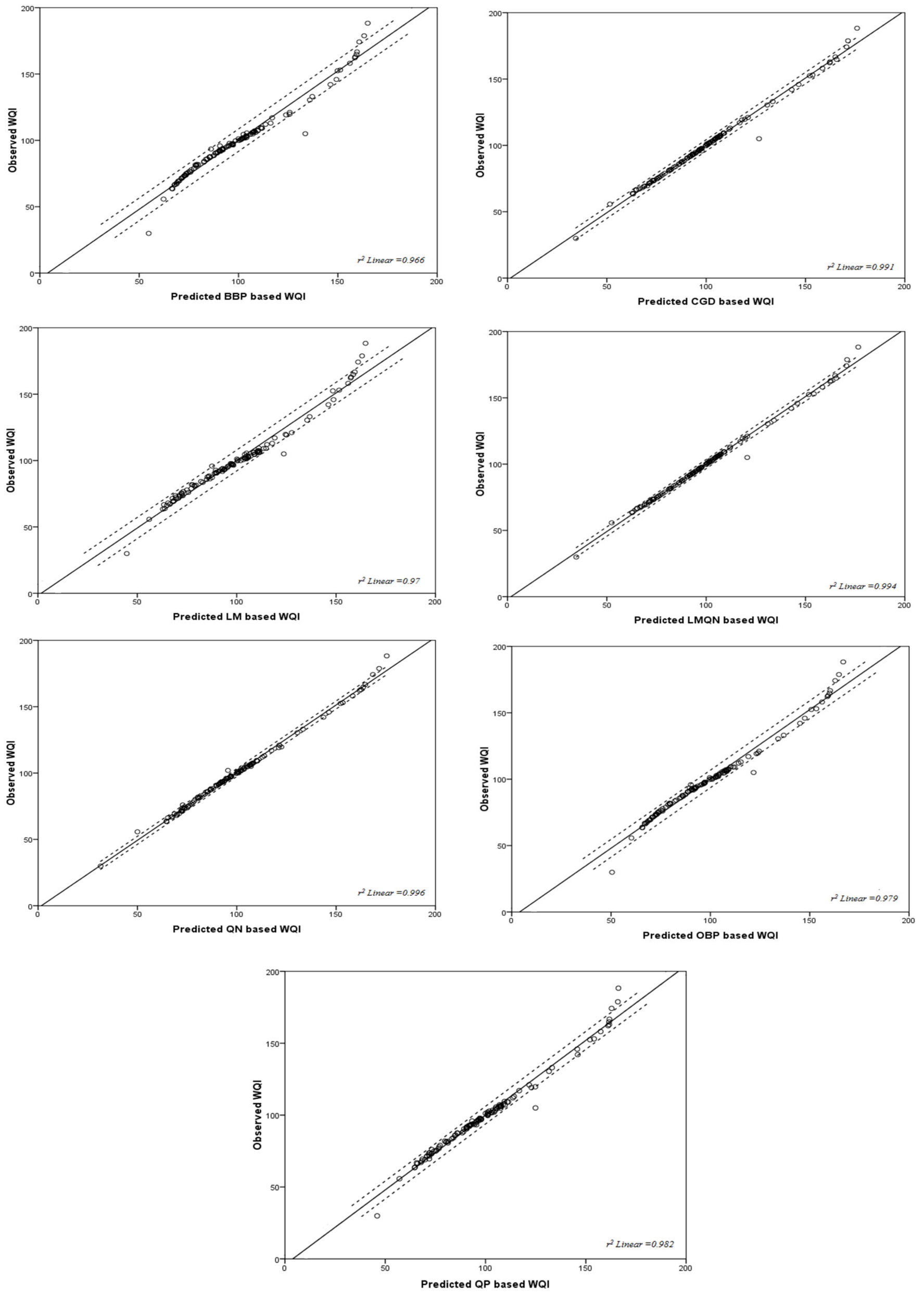
The results (

Table 5. Statistics of the ANN training algorithms-based MLR models.

		Coefficients						Collinearity Statistics
Model	Variable	B	Std. Error	Beta	r2	t	Sig.	Tolerance	VIF
WQIQP	Constant	23.344	0.970		0.985	24.072	0.00
	TDS	0.076	0.002	0.870		37.472	0.00	0.255	3.925
	Na	0.035	0.006	0.086		5.421	0.00	0.542	1.844
	Ca	0.083	0.018	0.090		4.704	0.00	0.376	2.660
WQICGD	Constant	20.733	0.631		0.994	32.845	0.00
	TDS	0.079	0.001	0.879		59.877	0.00	0.255	3.925
	Na	0.034	0.004	0.082		8.139	0.00	0.542	1.844
	Ca	0.084	0.011	0.088		7.294	0.00	0.376	2.660
WQIQN	Constant	22.644	1.140		0.978	19.859	0.00
	TDS	0.088	0.001	0.989		70.684	0.00	1.000	1.000
WQILMQN	Constant	22.478	0.858		0.987	26.207	0.00
	TDS	0.089	0.001	0.994		94.474	0.00	1.000	1.000
WQILM	Constant	−27.26	11.054		0.976	−2.466	0.015
	TDS	0.065	0.004	0.734		18.012	0.00	0.134	7.468
	Na	0.039	0.008	0.096		4.714	0.00	0.532	1.879
	Ca	0.12	0.024	0.128		5.082	0.00	0.351	2.847
	pH	5.813	1.368	0.066		4.250	0.00	0.919	1.088
	HCo3	0.027	0.008	0.066		3.399	0.00	0.589	1.697
	Cl	0.084	0.013	0.064		2.065	0.041	0.234	4.276
WQIOBP	Constant	25.287	1.194		0.974	21.173	0.00
	TDS	0.085	0.001	0.987		65.272	0.00	1.000	1.000
WQIBBP	Constant	24.159	1.231		0.975	19.619	0.00
	TDS	0.074	0.003	0.855		28.693	0.00	0.255	3.925
	Na	0.039	0.008	0.099		4.857	0.00	0.542	1.844
	Ca	0.084	0.022	0.093		3.771	0.00	0.376	2.660

) show that 97–99% of the total variations in the WQI that were predicted by the ANN training algorithms can be explained by the MLR models (Equations (5)–(11)). The MLR models indicated that TDS, Ca, and Na are important independent variables that contribute to the prediction of the WQI. The r² coefficient of the MLR models is significant at p < 0.05 and no collinearity was observed between the independent variables of the MLR models. Figure 3 illustrates the one-by-one relationship between the predicted and observed WQI.

Moreover, an intermodel comparison was conducted using the Akaike information criterion to screen the ANN training algorithm-based MLR models, to find the most appropriate one for predicting WQI.

3.3. Sensitivity Analysis

The ANN CGD training algorithm-based MLR model was determined to be the main model for predicting the water quality index in the source catchment (

Table 6. Results of the Akaike information criterion for ANN training algorithm-based MLR models.

ANN Training Algorithm-Based MLR Model	AICc	Ranking
CGD	82.59	1
QP	125.32	2
LM	139.37	3
QN	142.04	4
BBP	148.99	5
LMQN	361.32	6
OBP	415.60	7

). The results of the goodness of fit to determine the statistical distributions of the variables in the MLR model, together with the a priori and posteriori statistics of the statistical distributions, are shown in

Table 7. A priori and posteriori statistics of the statistical distribution of the ANN CGD training algorithm-based MLR model.

ANN Training Algorithm		Model Variable	Mean	Min	Max	S.D.	Variance
WQIcgd	A priori statistics	TDS	863.19	141	1785	297.91	710.75
		Ca	64.53	16.03	160.32	28.09	789.40
		Na	150.48	0	363.24	64.46	4155.73
	Posteriori statistics	Yobs.	99.15	34.4	175.97	26.66	710.75
		TDS	862.46	339.47	5219.1	307.39	94,488.3
		Ca	64.91	14.98	436.26	31.03	962.9
		Na	134.18	14.52	3234.0	83.92	7043.06
	Ysim.|Change in target variable for SA	TDS	99.40	58.08	443.58	24.28	589.7
		Ca	99.49	95.3	130.68	2.6	6.79
		Na	98.9	94.84	204.3	2.85	8.14

.

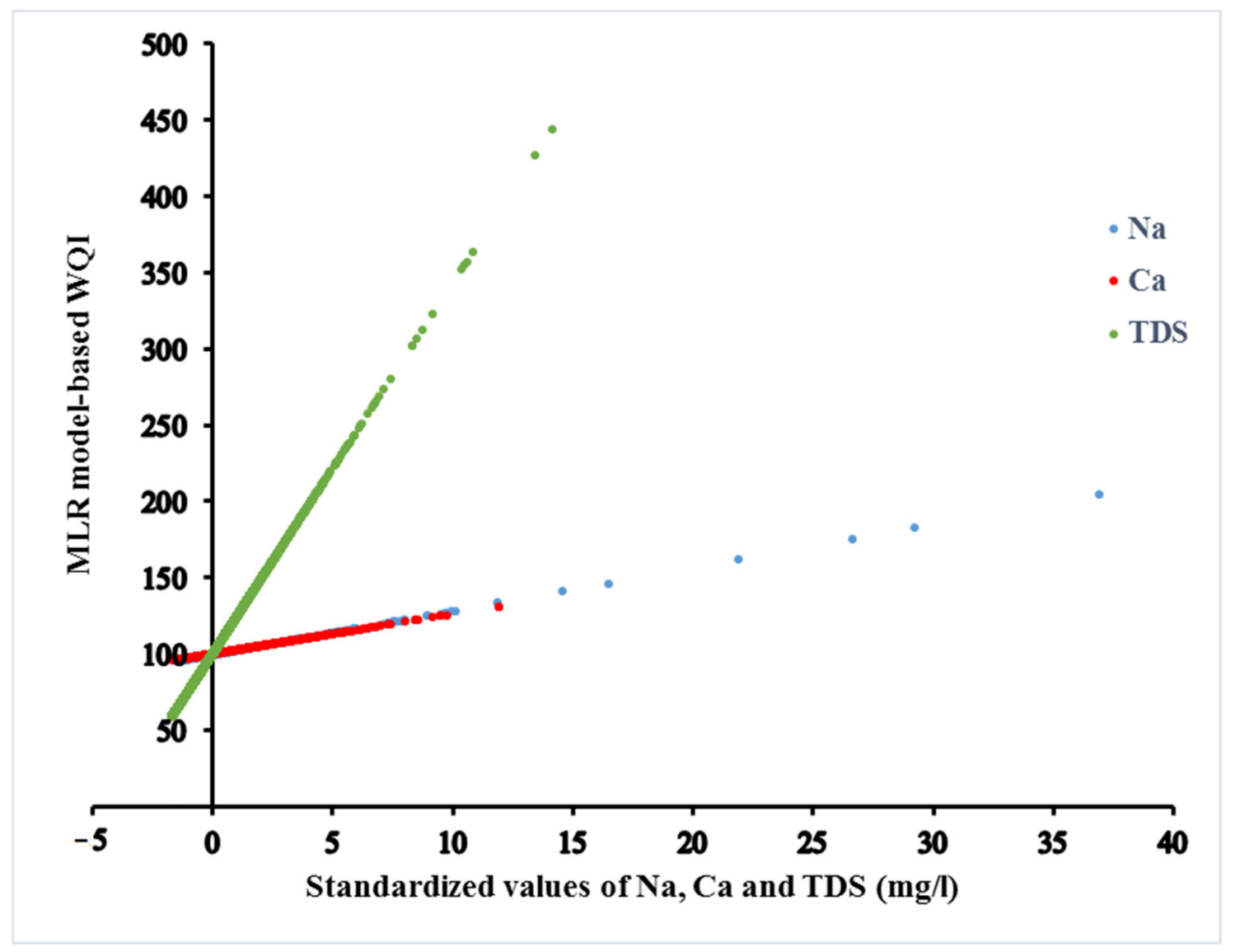
The slope of the lines (Figure 4) indicates how sensitive the responses of the ANN CGD training algorithm-based MLR model are, in relation to the change in a given variable, while the other variables were fixed by their average values. The results of the sensitivity analysis showed that the ANN CGD training algorithm-based MLR model is the most sensitive to change in the Ca variable, while the least sensitive is the TDS variable.

3.4. Uncertainty Analysis

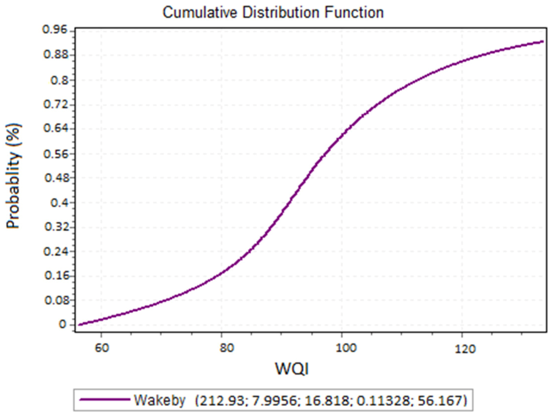
Monte Carlo simulations were performed to analyze the uncertainty of the ANN CGD training algorithm-based MLR model to the dependent and independent variables (

Table 8. Results of the statistical distribution for the ANN CGD training algorithm-based MLR model.

Statistics	Variable	Statistical Distribution	Komologrov Simirnov		Statistical Parameters
			Statistics	p-Value
	TDS	Wake by	0.07468	0.5	α = 2616 β = 8.1652 γ = 207.76 δ = 0.1286 ξ = 339.35
a prior	Ca	Erlang	0.07961	0.5	α =1.4052 β =2.1451 a = 22.445 b = 160.32
	Na	Wake by	0.05868	0.5	α = 524.58 β = 5.2938 γ = 36.524 δ = 0.1505 ξ = 24.138
posterior	Yobs.	Wake by	0.07673	0.5	α = 265.69 β = 8.1782 γ = 19.192 δ = 0.10217 ξ = 48.831
	YSim.	Wake by	0.0048	0.5	α = 201.36 β = 7.7886 γ = 16.748 δ = 0.11488 ξ = 57.049

). The cumulative density function (CDF), F(x), which expresses the random probability of variable X, evaluates a value less than or equal to the values of F (x) = Pr(X = x). In this study, the cumulative density function was considered to determine the probability that the output model functions are less than zero (Pr (Output) < 0), since only positive values can be acceptable for the water quality index. The behavior of the model can be investigated on the values of the cumulative density function. Consequently, the probability values of the cumulative density function for the variables Pr (Output) < 0 for the independent variables were carried out in the modeling, related to water quality (Figure 5). According to Figure 5, the probability that the ANN CGD training algorithm-based MLR model leads to negative values (Pr (Output) < 0) is equal to 0%.

3.5. Scaling the ANN CGD Training Algorithm-Based MLR Model

To up- and downscale the ANN CGD training algorithm-based MLR model, we applied Equations (12) (r² = 0.797) and (13) (r² = 0.995), respectively, which are based on the variable aggregation and disaggregation approach. The results of the up- and downscaling of the ANN CGD training algorithm-based MLR model are summarized in

Table 9. Results of the scaling of the ANN CGD training algorithm-based MLR model.

Catchment		Area (km2)	Mean Discharge (m3 s−1)	Upscaling		Downscaling
No.	Type			r2	MAE	r2	MAE
1	Very Large	1281.1	5.76	0.912	7.89	0.93	2.37
2		1801.17	4.42	0.63	9.63	0.871	5.00
3		2545.87	2.26	0.916	8.80	0.961	4.73
4		1511	1.68	0.958	8.26	0.995	2.16
mean ± sd.		1784.78 ± 550.2	3.53 ± 1.9	0.85 ± 0.15	8.45 ± 0.75	0.93 ± 0.05	3.56 ± 1.5
5	Large	977.84	4.63	0.961	10.18	0.973	2.60
6		581.65	1.78	0.672	11.86	0.972	2.35
7		539.44	0.05	0.553	32.74	0.949	7.44
mean ± sd.		699.64 ± 241.8	2.15 ± 2.31	0.73 ± 0.2	18.26 ± 12.57	0.96 ± 0.01	4.13 ± 2.87
8	Medium	181.63	0.09	0.875	7.10	0.994	1.61
9		131.6	0.67	0.578	3.33	0.921	3.27
10		554.4	2.36	0.864	7.17	0.98	1.90
11		348.41	2.00	0.78	6.51	0.957	2.04
12		152.1	1.50	0.902	2.93	0.968	1.13
13		380.04	0.23	0.949	8.87	0.998	1.50
14		425.98	0.36	0.929	18.41	0.993	3.34
15		156	0.42	0.495	13.98	0.968	2.71
mean ± sd.		291.27 ± 157.53	0.95 ± 0.87	0.79 ± 0.16	8.53 ± 5.26	0.97 ± 0.02	2.18 ± 0.82
16	Small	77.36	0.37	0.741	11.03	0.94	2.48
17		77.5	0.32	0.778	13.54	0.982	2.79
18		55.69	1.22	0.952	11.61	0.997	2.36
mean ± sd.		70.18 ± 12.55	0.63 ± 0.5	0.82 ± 0.11	12.06 ± 1.31	0.97 ± 0.03	2.54 ± 0.22
19	Very Small	42.54	0.12	0.81	14.53	0.975	3.82
20		12.23	0.09	0.599	15.18	0.86	3.73
21		25.62	0.33	0.809	13.90	0.842	4.33
22		8.42	0.08	0.985	15.21	0.997	3.61
23		43.02	0.22	0.892	10.96	0.988	2.30
24		31.32	0.09	0.604	12.98	0.99	2.01
25		38.67	0.49	0.502	13.99	0.964	3.19
mean ± sd.		28.83 ± 14.11	0.2 ± 0.15	0.74 ± 0.17	13.82 ± 1.48	0.94 ± 0.06	3.28 ± 0.84

. It shows that the aggregated MLR model (Equation (12)) could provide reliable performance in predicting the water quality index, since the r² coefficients of the WQI predictions range from 0.73 ± 0.2 for large catchments, to 0.85 ± 0.15 for very large catchments. However, for the disaggregated MLR model (Equation (13)), the r² coefficients of the WQI predictions vary from 0.93 ± 0.05 for very large catchments, to 0.97 ± 0.02 for medium catchments.

$${\mathrm{WQI}}_{\mathrm{cgd}}=0.616\left(\mathrm{Ca}\right)+0.196\left(\mathrm{Na}\right)+29.925$$

(12)

$${\mathrm{WQI}}_{\mathrm{cgd}}=0.086\left(\mathrm{TDS}\right)+0.032\left(\mathrm{Na}\right)+0.076\left(\mathrm{Ca}\right)-0.018\left({\mathrm{SO}}_4\right)+18.979$$

(13)

4. Discussion

The present study has shown that the use of ANN models to determine WQI is a very effective tool to predict the characteristics of river water quality (see, e.g., [75,76,77]). Our findings indicated that the ANN training algorithms can be reliable in predicting and simulating the WQI. Gupta et al. (2019) [76] suggested that ANN models could capture 89% of total variations in WQI, while Othman et al. (2020) [41] revealed that the ANN model could explain 97.78% of the total variations in water quality indices, demonstrating the relatively high performance of ANN training algorithms to predict and simulate water quality [12,65,78]. The applicability of the ANN CGD training algorithm to predict water quality was also confirmed by the findings of Abbaszadeh (2016) [79]. Bafithite (2018) [80] compared the ANN LM and CGD training algorithms to simulate river flow, showing that the ANN CGD training algorithm is more appropriate than any of the other algorithms. The conjugate gradient descent training algorithm of ANN is one of the most frequently used algorithms, due to its simplicity, numerical efficiency, and very low memory requirements for the efficient training tasks of neural networks [81].

Many studies (see, e.g., [82,83,84]) show that the application of ANN models can provide reliable results when predicting water quality indices. The regression model that was developed using the output of the ANN CGD training algorithm as the dependent variable and a set of water quality variables as the independent variables can show the required efficacy in predicting WQI, in the absence of sufficient data and without trapping users in complex calculations, such as artificial intelligence, which is in line with the findings of Haverkamp et al. (2002) [23]. In other words, we found that the regression model is appropriate for use in scaling, as indicated by Zhang et al. (2020) [27] and Zirlewagen and Von Wilpert (2010) [28]. Although several studies [20,22,32] have indicated that regression models may not produce reliable upscaling performance, our findings revealed that reliable performance can be achieved, which is consistent with Henze et al. (2020) [85]. The evaluation of aggregated and disaggregated MLR models to predict water quality indices in target catchments showed that they could significantly explain the water quality indices. Therefore, it can be considered an alternative and cost-effective tool for predicting and scaling river water quality, in terms of time constraints and limited field data.

5. Conclusions

Our findings revealed that the up- and downscaling of the ANN-based MLR model, on the basis of the variable aggregation and disaggregation, can be considered as one of the most effective approaches, by which water quality index can be predicted in the catchments that lack sufficient data, since the performance of the up- and downscaled model varied between 0.93 and 0.97, depending on to which types of catchments those models were applied. The upscaled models can provide us with a tool for assessing the impacts of the strategies and policies at the national level, in general, and at basin level, in particular. They can stop strategies and policies that are detrimental to water resource sustainability from being translated into plans, programs, and, more importantly, projects that inherently degrade the environment. The downscaled models can support local decision making in socio-ecological management. Although we found that the upscaled and downscaled models are appropriate to predict the WQI in the southern basin of the Caspian Sea, it is suggested that the proposed methodology be extended to other basins of the country.

It is obvious that the modeling of water quality characteristics varies, depending on geographical conditions and at different scales, which makes it possible to use hybrid approaches and models to optimize the model and reduce errors. Considering that river water quality is affected by the rainfall-runoff process, and the process is driven by factors, including but not limited to evaporation, vegetation, soil, and geology, examining the contribution of the driving forces in river water quality, using different intelligence models, such as model tree, gene expression programming, support vector machine, multivariate adaptive regression spline, adaptive neurofuzzy inference system, and evolutionary polynomial regression, can increase our understanding of this issue.

References

- Aalipour Erdi, M.; Gasempour Niari, H.; Meshkini, S.R.M.; Foroug, S. Surveying drinking water quality (Balikhlou River, Ardabil Province, Iran). Appl. Water Sci. 2018, 8, 34. [Google Scholar] [CrossRef] [Green Version]
- Singh, K.P.; Malik, A.; Sinha, S. Water quality assessment and apportionment of pollution sources of Gomti river (India) using multivariate statistical techniques—a case study. Anal. Chim. Acta 2005, 538, 355–374. [Google Scholar] [CrossRef]
- Taylor, S.D.; He, Y.; Hiscock, K.M. Modelling the impacts of agricultural management practices on river water quality in Eastern England. J. Environ. Manag. 2016, 180, 147–163. [Google Scholar] [CrossRef] [PubMed] [Green Version]
- Aalipour, M.; Antczak, E.; Dostál, T.; Jabbarian Amiri, B. Influences of Landscape Configuration on River Water Quality. Forests 2022, 13, 222. [Google Scholar] [CrossRef]
- Aalipour Ardi, M.; Jabbarian Amiri, B. Investigating the Effects of Land Use/Land Cover Composition on River Water Quality. J. Civ. Environ. Eng. 2021, 51, 83–93. [Google Scholar]
- Mishra, B.K.; Regmi, R.K.; Masago, Y.; Fukushi, K.; Kumar, P.; Saraswat, C. Assessment of Bagmati river pollution in Kathmandu Valley: Scenario-based modeling and analysis for sustainable urban development. Sustain. Water Qual. Ecol. 2017, 9, 67–77. [Google Scholar] [CrossRef]
- Shakhman, I.; Bystriantseva, A. Water Quality Assessment of the Surface Water of the Southern Bug River Basin by Complex Indices. J. Ecol. Eng. 2021, 22, 195–205. [Google Scholar] [CrossRef]
- Witek, Z.; Jarosiewicz, A. Long-Term Changes in Nutrient Status of River Water. Pol. J. Environ. Stud. 2009, 18, 1177–1184. [Google Scholar]
- Reza, R.; Singh, G. Heavy metal contamination and its indexing approach for river water. Int. J. Environ. Sci. Technol. 2010, 7, 785–792. [Google Scholar] [CrossRef] [Green Version]
- Tiri, A.; Belkhiri, L.; Mouni, L. Evaluation of surface water quality for drinking purposes using fuzzy inference system. Groundw. Sustain. Dev. 2018, 6, 235–244. [Google Scholar] [CrossRef]
- Bachmair, S.; Weiler, M. Interactions and connectivity between runoff generation processes of different spatial scales. Hydrol. Processes 2014, 28, 1916–1930. [Google Scholar] [CrossRef]
- won Seo, I.; Yun, S.H.; Choi, S.Y. Forecasting water quality parameters by ANN model using pre-processing technique at the downstream of Cheongpyeong Dam. Proc. Eng. 2016, 154, 1110–1115. [Google Scholar]
- Rios Rivera, M.A. Upscaling of Point-Scale Groundwater Recharge Measurements Using Machine Learning: A Case Study in New Zealand and Colombia. Ph.D. Thesis, Lincoln University, Lincoln, New Zealand, 2019. [Google Scholar]
- Hamid, A.; Bhat, S.U.; Jehangir, A. Local determinants influencing stream water quality. Appl. Water Sci. 2020, 10, 24. [Google Scholar] [CrossRef] [Green Version]
- Yang, L.; Schnabel, T.; Bennett, P.N.; Dumais, S. Local Factor Models for Large-Scale Inductive Recommendation. In Proceedings of the Fifteenth ACM Conference on Recommender Systems, Amsterdam, The Netherlands, 27 September–1 October 2021; pp. 252–262. [Google Scholar]
- Verhoeven, J.T.; Arheimer, B.; Yin, C.; Hefting, M.M. Regional and global concerns over wetlands and water quality. Trends Ecol. Evol. 2006, 21, 96–103. [Google Scholar] [CrossRef]
- Kanownik, W.; Policht-Latawiec, A.; Fudała, W. Nutrient pollutants in surface water—Assessing trends in drinking water resource quality for a regional city in Central Europe. Sustainability 2019, 11, 1988. [Google Scholar] [CrossRef] [Green Version]
- Read, E.K.; Carr, L.; De Cicco, L.; Dugan, H.A.; Hanson, P.C.; Hart, J.A.; Kreft, J.; Read, J.S.; Winslow, L.A. Water quality data for national-scale aquatic research: The Water Quality Portal. Water Resour. Res. 2017, 53, 1735–1745. [Google Scholar] [CrossRef]
- Troy, T.J.; Wood, E.F.; Sheffield, J. An efficient calibration method for continental-scale land surface modeling. Water Resour. Res. 2008, 44, 1–13. [Google Scholar] [CrossRef]
- Fritsch, M.; Lischke, H.; Meyer, K.M. Scaling methods in ecological modelling. Methods Ecol. Evol. 2020, 11, 1368–1378. [Google Scholar] [CrossRef]
- Taghizadeh-Mehrjardi, R. Spatial down-scaling in digital mapping of soil organic carbon using auxiliary data (case study: Baneh region). J. Agric. Eng. Soil Sci. Agric. Mech. 2017, 40, 71–85. [Google Scholar]
- Yuan, L.; Sinshaw, T.; Forshay, K.J. Review of watershed-scale water quality and nonpoint source pollution models. Geosciences 2020, 10, 25. [Google Scholar] [CrossRef] [Green Version]
- Haverkamp, S.; Srinivasan, R.; Frede, H.; Santhi, C. Subwatershed spatial analysis tool: Discretization of a distributed hydrologic model by statistical criteria 1. J. Am. Water Resour. Assoc. 2002, 38, 1723–1733. [Google Scholar] [CrossRef]
- Larsen, R.K.; Swartling, Å.G.; Powell, N.; May, B.; Plummer, R.; Simonsson, L.; Osbeck, M. A framework for facilitating dialogue between policy planners and local climate change adaptation professionals: Cases from Sweden, Canada and Indonesia. Environ. Sci. Policy 2012, 23, 12–23. [Google Scholar] [CrossRef]
- Wilby, R.L.; Wigley, T.M. Downscaling general circulation model output: A review of methods and limitations. Prog. Phys. Geogr. 1997, 21, 530–548. [Google Scholar] [CrossRef]
- Karger, D.N.; Conrad, O.; Böhner, J.; Kawohl, T.; Kreft, H.; Soria-Auza, R.W.; Zimmermann, N.E.; Linder, H.P.; Kessler, M. Climatologies at high resolution for the earth’s land surface areas. Sci. Data 2017, 4, 170122. [Google Scholar] [CrossRef] [Green Version]
- Zhang, L.; Xu, Y.; Meng, C.; Li, X.; Liu, H.; Wang, C. Comparison of statistical and dynamic downscaling techniques in generating high-resolution temperatures in China from CMIP5 GCMs. J. Appl. Meteorol. Climatol. 2020, 59, 207–235. [Google Scholar] [CrossRef]
- Zirlewagen, D.; von Wilpert, K. Upscaling of environmental information: Support of land-use management decisions by spatio-temporal regionalization approaches. Environ. Manag. 2010, 46, 878–893. [Google Scholar] [CrossRef]
- Leitão, P.J.; Schwieder, M.; Pötzschner, F.; Pinto, J.R.; Teixeira, A.M.; Pedroni, F.; Sanchez, M.; Rogass, C.; Van Der Linden, S.; Bustamante, M.M. From sample to pixel: Multi-scale remote sensing data for upscaling aboveground carbon data in heterogeneous landscapes. Ecosphere 2018, 9, e02298. [Google Scholar] [CrossRef] [Green Version]
- Snell, R.S.; Huth, A.; Nabel, J.E.; Bocedi, G.; Travis, J.M.; Gravel, D.; Bugmann, H.; Gutiérrez, A.G.; Hickler, T.; Higgins, S.I. Using dynamic vegetation models to simulate plant range shifts. Ecography 2014, 37, 1184–1197. [Google Scholar] [CrossRef]
- Wagener, T.; Sivapalan, M.; Troch, P.; Woods, R. Catchment classification and hydrologic similarity. Geogr. Compass 2007, 1, 901–931. [Google Scholar] [CrossRef]
- Yang, S.; Liang, M.; Qin, Z.; Qian, Y.; Li, M.; Cao, Y. A novel assessment considering spatial and temporal variations of water quality to identify pollution sources in urban rivers. Sci. Rep. 2021, 11, 8714. [Google Scholar] [CrossRef]
- Buck, O.; Niyogi, D.K.; Townsend, C.R. Scale-dependence of land use effects on water quality of streams in agricultural catchments. Environ. Pollut. 2004, 130, 287–299. [Google Scholar] [CrossRef] [PubMed]
- Uriarte, M.; Yackulic, C.B.; Lim, Y.; Arce-Nazario, J.A. Influence of land use on water quality in a tropical landscape: A multi-scale analysis. Landsc. Ecol. 2011, 26, 1151–1164. [Google Scholar] [CrossRef] [PubMed] [Green Version]
- Zhou, B.; Xu, Y.; Vogt, R.D.; Lu, X.; Li, X.; Deng, X.; Yue, A.; Zhu, L. Effects of land use change on phosphorus levels in surface waters—a case study of a watershed strongly influenced by agriculture. Water Air Soil Pollut. 2016, 227, 160. [Google Scholar] [CrossRef]
- Mineau, M.M.; Wollheim, W.M.; Stewart, R.J. An index to characterize the spatial distribution of land use within watersheds and implications for river network nutrient removal and export. Geophys. Res. Lett. 2015, 42, 6688–6695. [Google Scholar] [CrossRef] [Green Version]
- Öz, N.; Topal, B.; Uzun, H.I. Prediction of water quality in Riva River watershed. Ecol. Chem. Eng. S 2019, 26, 727–742. [Google Scholar]
- Chen, Y.; Song, L.; Liu, Y.; Yang, L.; Li, D. A review of the artificial neural network models for water quality prediction. Appl. Sci. 2020, 10, 5776. [Google Scholar] [CrossRef]
- Malik, A.; Kumar, A.; Kisi, O.; Shiri, J. Evaluating the performance of four different heuristic approaches with Gamma test for daily suspended sediment concentration modeling. Environ. Sci. Pollut. Res. 2019, 26, 22670–22687. [Google Scholar] [CrossRef]
- Noori, R.; Karbassi, A.; Mehdizadeh, H.; Vesali-Naseh, M.; Sabahi, M. A framework development for predicting the longitudinal dispersion coefficient in natural streams using an artificial neural network. Environ. Prog. Sustain. Energy 2011, 30, 439–449. [Google Scholar] [CrossRef]
- Othman, F.; Alaaeldin, M.; Seyam, M.; Ahmed, A.N.; Teo, F.Y.; Ming Fai, C.; Afan, H.A.; Sherif, M.; Sefelnasr, A.; El-Shafie, A. Efficient river water quality index prediction considering minimal number of inputs variables. Eng. Appl. Comput. Fluid Mech. 2020, 14, 751–763. [Google Scholar] [CrossRef]
- Bandyopadhyay, G.; Chattopadhyay, S. Single hidden layer artificial neural network models versus multiple linear regression model in forecasting the time series of total ozone. Int. J. Env. Sci. Technol. 2007, 4, 141–149. [Google Scholar] [CrossRef] [Green Version]
- Wang, J.; Sui, J.; Guo, L.; Karney, B.; Jüpner, R. Forecast of water level and ice jam thickness using the back propagation neural network and support vector machine methods. Int. J. Env. Sci. Technol. 2010, 7, 215–224. [Google Scholar] [CrossRef] [Green Version]
- Yilmaz, I.; Kaynar, O. Multiple regression, ANN (RBF, MLP) and ANFIS models for prediction of swell potential of clayey soils. Expert Syst. Appl. 2011, 38, 5958–5966. [Google Scholar] [CrossRef]
- Chau, K. A review on integration of artificial intelligence into water quality modelling. Mar. Pollut. Bull. 2006, 52, 726–733. [Google Scholar] [CrossRef] [Green Version]
- Singh, K.; Basant, A.; Malik, A.; Jain, G. Artificial neural network modeling of the river water quality, a case study. Ecol. Model. 2009, 220, 888–895. [Google Scholar] [CrossRef]
- Nourani, V.; Khanghah, T.R.; Sayyadi, M. Application of the Artificial Neural Network to monitor the quality of treated water. Int. J. Manag. Inf. Technol. 2013, 3, 38–45. [Google Scholar] [CrossRef]
- Emamgholizadeh, S.; Kashi, H.; Marofpoor, I.; Zalaghi, E. Prediction of water quality parameters of Karoon River (Iran) by artificial intelligence-based models. Int. J. Environ. Sci. Technol. 2014, 11, 645–656. [Google Scholar] [CrossRef] [Green Version]
- Medeiros, A.C.; Faial, K.R.F.; Faial, K.d.C.F.; da Silva Lopes, I.D.; de Oliveira Lima, M.; Guimarães, R.M.; Mendonça, N.M. Quality index of the surface water of Amazonian rivers in industrial areas in Pará, Brazil. Mar. Pollut. Bull. 2017, 123, 156–164. [Google Scholar] [CrossRef]
- Horton, R.K. An index number system for rating water quality. J. Water Pollut. Control. Fed. 1965, 37, 300–306. [Google Scholar]
- Brown, R.M.; McClelland, N.I.; Deininger, R.A.; Tozer, R.G. A water quality index-do we dare. Water Sew. Work. 1970, 117, 339–343. [Google Scholar]
- Najafzadeh, M.; Homaei, F.; Farhadi, H. Reliability assessment of water quality index based on guidelines of national sanitation foundation in natural streams: Integration of remote sensing and data-driven models. Artif. Intell. Rev. 2021, 54, 4619–4651. [Google Scholar] [CrossRef]
- Uddin, M.G.; Nash, S.; Olbert, A.I. A review of water quality index models and their use for assessing surface water quality. Ecol. Indic. 2021, 122, 107218. [Google Scholar] [CrossRef]
- Noori, R.; Berndtsson, R.; Hosseinzadeh, M.; Adamowski, J.F.; Abyaneh, M.R. A critical review on the application of the National Sanitation Foundation Water Quality Index. Environ. Pollut. 2019, 244, 575–587. [Google Scholar] [CrossRef]
- Wagh, V.; Panaskar, D.; Muley, A.; Mukate, S. Groundwater suitability evaluation by CCME WQI model for Kadava river basin, Nashik, Maharashtra, India. Modeling Earth Syst. Environ. 2017, 3, 557–565. [Google Scholar] [CrossRef]
- Şener, Ş.; Şener, E.; Davraz, A. Evaluation of water quality using water quality index (WQI) method and GIS in Aksu River (SW-Turkey). Sci. Total Environ. 2017, 584, 131–144. [Google Scholar] [CrossRef]
- Yidana, S.M.; Banoeng-Yakubo, B.; Akabzaa, T.M. Analysis of groundwater quality using multivariate and spatial analyses in the Keta basin, Ghana. J. Afr. Earth Sci. 2010, 58, 220–234. [Google Scholar] [CrossRef]
- Vasant, W.; Dipak, P.; Aniket, M.; Ranjitsinh, P.; Shrikant, M.; Nitin, D.; Manesh, A.; Abhay, V. GIS and statistical approach to assess the groundwater quality of Nanded Tehsil, (MS) India. In Proceedings of the First International Conference on Information and Communication Technology for Intelligent Systems; Springer: Cham, Switzerland, 2016; Volume 1, pp. 409–417. [Google Scholar]
- Singh, B. Prediction of the sodium absorption ratio using data-driven models: A case study in Iran. Geol. Ecol. Landsc. 2020, 4, 1–10. [Google Scholar] [CrossRef] [Green Version]
- Singh, B.; Sihag, P.; Singh, V.P.; Sepahvand, A.; Singh, K. Soft computing technique-based prediction of water quality index. Water Supply 2021, 21, 4015–4029. [Google Scholar] [CrossRef]
- Saeedi, M.; Abessi, O.; Sharifi, F.; Meraji, H. Development of groundwater quality index. Environ. Monit. Assess. 2010, 163, 327–335. [Google Scholar] [CrossRef]
- Csábrági, A.; Molnár, S.; Tanos, P.; Kovács, J.; Molnár, M.; Szabó, I.; Hatvani, I.G. Estimation of dissolved oxygen in riverine ecosystems: Comparison of differently optimized neural networks. Ecol. Eng. 2019, 138, 298–309. [Google Scholar] [CrossRef]
- Barzegar, R.; Moghaddam, A.A.; Adamowski, J.; Ozga-Zielinski, B. Multi-step water quality forecasting using a boosting ensemble multi-wavelet extreme learning machine model. Stoch. Environ. Res. Risk Assess. 2018, 32, 799–813. [Google Scholar] [CrossRef]
- Shi, I. Reducing prediction error by transforming input data for neural networks. J. Comput. Civ. Eng. 2000, 14, 109–116. [Google Scholar] [CrossRef]
- Kadam, A.; Wagh, V.; Muley, A.; Umrikar, B.; Sankhua, R. Prediction of water quality index using artificial neural network and multiple linear regression modelling approach in Shivganga River basin, India. Model. Earth Syst. Environ. 2019, 5, 951–962. [Google Scholar] [CrossRef]
- Panchal, G.; Ganatra, A.; Kosta, Y.; Panchal, D. Searching most efficient neural network architecture using Akaike’s information criterion (AIC). Int. J. Comput. Appl. 2010, 1, 41–44. [Google Scholar] [CrossRef]
- Sheela, K.G.; Deepa, S.N. Review on methods to fix number of hidden neurons in neural networks. Math. Probl. Eng. 2013, 2013, 425740. [Google Scholar] [CrossRef] [Green Version]
- Thomas, V.; Pedregosa, F.; van Merriënboer, B.; Mangazol, P.-A.; Bengio, Y.; Le Roux, N. Information matrices and generalization. arXiv 2019, arXiv:1906.07774. [Google Scholar]
- Neter, J.; Kutner, M.H.; Nachtsheim, C.J.; Wasserman, W. Applied Linear Statistical Models; Irwin Chicago: Chicago, IL, USA, 1996; Volume 4. [Google Scholar]
- Chatterjee, S.; Hadi, A.S. Regression Analysis by Example; John Wiley & Sons: Hoboken, NJ, USA, 2015. [Google Scholar]
- Ahearn, D.S.; Sheibley, R.W.; Dahlgren, R.A.; Anderson, M.; Johnson, J.; Tate, K.W. Land use and land cover influence on water quality in the last free-flowing river draining the western Sierra Nevada, California. J. Hydrol. 2005, 313, 234–247. [Google Scholar] [CrossRef]
- Dotto, C.B.; Mannina, G.; Kleidorfer, M.; Vezzaro, L.; Henrichs, M.; McCarthy, D.T.; Freni, G.; Rauch, W.; Deletic, A. Comparison of different uncertainty techniques in urban stormwater quantity and quality modelling. Water Res. 2012, 46, 2545–2558. [Google Scholar] [CrossRef]
- Saltelli, A.; Tarantola, S.; Campolongo, F. Sensitivity analysis as an ingredient of modeling. Stat. Sci. 2000, 15, 377–395. [Google Scholar]
- Amiri, B.J.; Gao, J.; Fohrer, N.; Adamowski, J.; Huang, J. Examining lag time using the landscape, pedoscape and lithoscape metrics of catchments. Ecol. Indic. 2019, 105, 36–46. [Google Scholar] [CrossRef]
- Sakizadeh, M. Artificial intelligence for the prediction of water quality index in groundwater systems. Modeling Earth Syst. Environ. 2016, 2, 8. [Google Scholar] [CrossRef]
- Gupta, R.; Singh, A.; Singhal, A. Application of ANN for water quality index. Int. J. Mach. Learn. Comput. 2019, 9, 688–693. [Google Scholar] [CrossRef]
- Aldhyani, T.H.; Al-Yaari, M.; Alkahtani, H.; Maashi, M. Water quality prediction using artificial intelligence algorithms. Appl. Bionics Biomech. 2020, 2020, 6659314. [Google Scholar] [CrossRef]
- Vasanthi, S.S.; Kumar, S.A. Application of artificial neural network techniques for predicting the water quality index in the Parakai Lake, Tamil Nadu, India. Appl. Ecol. Environ. Res. 2019, 17, 1947–1958. [Google Scholar] [CrossRef]
- Shahri, A.A. An optimized artificial neural network structure to predict clay sensitivity in a high landslide prone area using piezocone penetration test (CPTu) data: A case study in southwest of Sweden. Geotech. Geol. Eng. 2016, 34, 745–758. [Google Scholar] [CrossRef]
- Bafitlhile, T.M.; Li, Z.; Li, Q. Comparison of levenberg marquardt and conjugate gradient descent optimization methods for simulation of streamflow using artificial neural network. Adv. Ecol. Environ. Res. 2018, 3, 217–237. [Google Scholar]
- Livieris, I.E.; Pintelas, P. An advanced conjugate gradient training algorithm based on a modified secant equation. Int. Sch. Res. Not. 2012, 2012, 486361. [Google Scholar] [CrossRef] [Green Version]
- Kim, S.E.; Seo, I.W. Artificial Neural Network ensemble modeling with conjunctive data clustering for water quality prediction in rivers. J. Hydro-Environ. Res. 2015, 9, 325–339. [Google Scholar] [CrossRef]
- Tomas, D.; Čurlin, M.; Marić, A.S. Assessing the surface water status in Pannonian ecoregion by the water quality index model. Ecol. Indic. 2017, 79, 182–190. [Google Scholar] [CrossRef]
- Avila, R.; Horn, B.; Moriarty, E.; Hodson, R.; Moltchanova, E. Evaluating statistical model performance in water quality prediction. J. Environ. Manag. 2018, 206, 910–919. [Google Scholar] [CrossRef]
- Henze, J.; Siefert, M.; Bremicker-Trübelhorn, S.; Asanalieva, N.; Sick, B. Probabilistic upscaling and aggregation of wind power forecasts. Energy Sustain. Soc. 2020, 10, 15. [Google Scholar] [CrossRef] [Green Version]
Figure 1.
Geographical location of the source catchment.
Figure 2.
Geographical location of the target catchments.
Figure 3.
Predicted versus observed WQI for the ANN training algorithms-based MLR models.
Figure 4.
Slope of the line for the variables of the ANN CGD training algorithm-based MLR model.
Figure 5.
The cumulative density function for the WQI that was simulated by the ANN CGD training algorithm-based MLR model.