
On Hypsometric Curve and Morphological Analysis of the Collapsed Irrigation Reservoirs


1
Department of Civil Engineering, Inha University, Incheon 22201, Korea
2
Institute of Water Resources System, Inha University, Incheon 22201, Korea
*
Author to whom correspondence should be addressed.
Water 2022, 14(6), 907; https://doi.org/10.3390/w14060907
Submission received: 24 December 2021
/
Revised: 3 March 2022
/
Accepted: 11 March 2022
/
Published: 14 March 2022
(This article belongs to the Section Hydraulics and Hydrodynamics)
Abstract
:The impact of irrigation reservoirs requires investigation through hydrological analysis to identify the flood control functions of these reservoirs. However, there is insufficient information concerning important geographical, morphological, and topographic characteristics, such as the reservoir cross-section. Therefore, this study aimed to identify the morphological and topographic characteristics of reservoirs using geographical information instead of measurement data. Ten reservoirs, including the Ga-Gog reservoir located in Miryang City, South Korea, were selected. The topographic information of the reservoirs was obtained using topographic maps and GIS techniques. Based on this information, the volume (V)-area (A)-depth (H) relationship and the hypsometric curve (HC) according to the relative area (a/A) and relative height (h/H) were created. A comparison of the reservoir volume, estimated using topographic information, with the measured volume revealed an error rate between 0.23% and 14.27%. In addition, two collapsed reservoirs located near Miryang City were investigated by creating V-A-H relationships and HCs using topographic information. The morphological characteristics of the reservoirs were identified by analyzing the (1) morphology index, (2) full water storage area-levee height relationship, and (3) full water storage area relationship. The analysis results showed that the collapsed reservoirs had high water depth and a large area relative to other reservoirs. Similar types of reservoirs were grouped by conducting a cluster analysis using basic properties such as the basin area, storage, and levee height. The cluster analysis results, based on HC analysis, grouped the reservoirs into three shapes: convex upward (youthful stage), relatively flat (mature stage), and convex downward (old stage). The HCs of the collapsed reservoirs exhibited a convex downward shape, indicating that they were subjected to considerable erosion due to aging. Moreover, this considerable erosion caused a large quantity of sediment to accumulate in the reservoirs, resulting in an insufficient allowable storage capacity of the reservoir because the flood control capacity was reduced, which may have led to their collapse during heavy rainfalls. Therefore, the identification of potential causes of reservoir collapse through the morphological characteristics and HCs of reservoirs are expected to support the operation and management of reservoirs to reduce flood damage.
1. Introduction
During the summer rainy season, water from precipitation in the form of heavy rainfall and typhoons is stored for use in the following year. In this way the water supply is secured, and water resources are managed through hydraulic facilities such as dam reservoirs that provide water and irrigation reservoirs for agriculture [1,2,3,4,5]. The influence of climate change is observed through the increased variability of precipitation and an imbalance in precipitation by region. Consequently, reservoirs in different regions are becoming more vulnerable to either droughts or floods. In particular, flood damage caused by the collapse of irrigation reservoirs occurs because rainfall is more frequent and has an increased rainfall intensity [6].
According to the National Disaster Management Research Institute, there are 16,791 reservoirs in South Korea, including 3406 reservoirs managed by the Korea Rural Community Corporation and 13,385 reservoirs managed by local governments. These reservoirs, having individual properties, vary depending on their topographic characteristics at time of completion [7].
Research on the hydraulic and hydrological analyses of reservoirs and their impact are necessary to implement drought and flood control, which is a function of reservoirs. Basic research on the topographic and morphological characteristics of reservoirs is important for accurate research [8]. While reservoir storage rates are monitored and the systematic management of reservoirs is maintained by the Korea Rural Community Corporation, there is insufficient supervision of small irrigation reservoirs that are managed by local governments. Many of the existing irrigation reservoirs in Korea are more than 50 years old [6,9], and these are small reservoirs with irrigation scales of 100 ha (0.01) or less. In addition, reservoirs have been inefficiently managed because of limited management personnel and considerable cost requirements [10]. Reservoirs, located in different parts of the country, exhibit different damage patterns during heavy rainfall events and have different shapes and characteristics. The flood damage patterns of irrigation reservoirs due to heavy rainfall are correlated to the topographic and physical factors of the reservoirs. Therefore, it is necessary to analyze the topography of the reservoirs and identify their morphological and physical characteristics [8,11,12].
Precision measuring instruments have been used in recent years to efficiently manage reservoirs by accurately quantifying properties such as area by water depth and the storage capacity. According to previous studies, manned and unmanned boats equipped with GPS and water depth sensors are used to measure the topography (area by water depth) and storage capacity of reservoirs [13,14,15,16,17,18]. However, these accurate reservoir property measurements, such as the area and storage capacity, necessitate considerable time and cost. In addition, as reservoirs are located in mountainous areas, access is a challenge for water depth-measuring equipment. Therefore, in this study, the water depth and area were obtained using topographic maps and GIS techniques. Using these data, an attempt was made to apply the hypsometric curve (HC), normally used for river basins, to quantitatively analyze the topographic and morphological characteristics of reservoirs.
Langbein et al. [19] used the HC to identify the topographic characteristics of basins in the northeastern United States. In addition, HCs were created by identifying the area by water depth, and the storage capacity using reservoir topographic information; thus, the topographic and morphological characteristics of these basins were identified and used as basic data [20,21,22,23]. The morphology index and HC are important information for researching reservoir topographic characteristics, and studies are required to quantitatively investigate topographic characteristics [24,25,26,27,28,29,30,31].
Should reservoir topographic and morphological characteristics be reliably identified through quantitative data obtained from topographic maps and GIS techniques, topographic information on reservoirs located in mountainous or remote areas with poor accessibility could be indirectly obtained. In addition, the topographic information obtained could be used for hydraulic and hydrological analyses, and for reservoir management.
Therefore, the purpose of this study was to construct the geometry of reservoirs using their topographic information and to evaluate its accuracy by comparing it with measured data and volumes of the reservoirs. In addition, HCs were created for reservoirs to understand their geometry and to identify the area by elevation and storage capacity. Moreover, an attempt was made to present the morphology index quantitatively through relational analysis using basic reservoir properties, such as the storage capacity and full water area, and to group similar types of reservoirs through cluster analysis. Based on this, topographic and morphological analyses of reservoirs that collapsed due to flooding were conducted to identify the potential causes of collapse.
2. Methodology and Material
2.1. Study Area
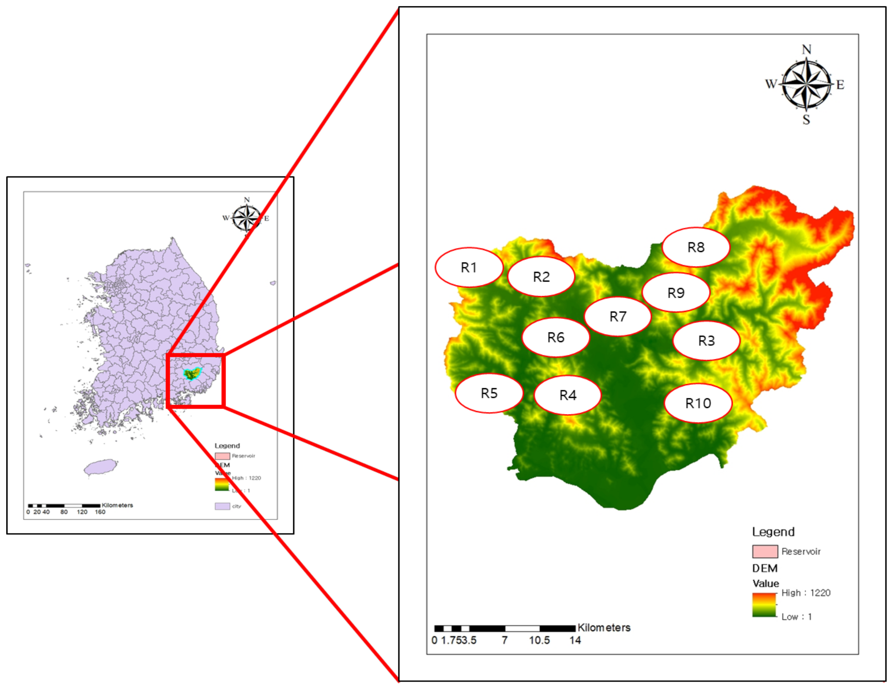
Ten reservoirs were selected for this study, including the Ga-Gog reservoir located in Miryang City, Gyeongsangnam Province. The total storage capacity was defined as the height from the bottom of the reservoir to full water level. As the dead storage levels could not be identified, the total storage volumes were compared and analyzed. The locations of the ten reservoirs, including the Ga-Gog Reservoir, are shown in Figure 1. The names of the ten reservoirs are R(1): Ga-Gog, R(2): Nae-Gog, R(3): Dae-Gog, R(4): Sam-Son, R(5): Deog-Am, R(6): Un-Jeong, R(7): Yong-Po, R(8): O-Cho, R(9): Ga-Gog2, and R(10): U-Gog2.
2.2. The Area-Volume Relationship of Reservoirs According to the Depth of Water
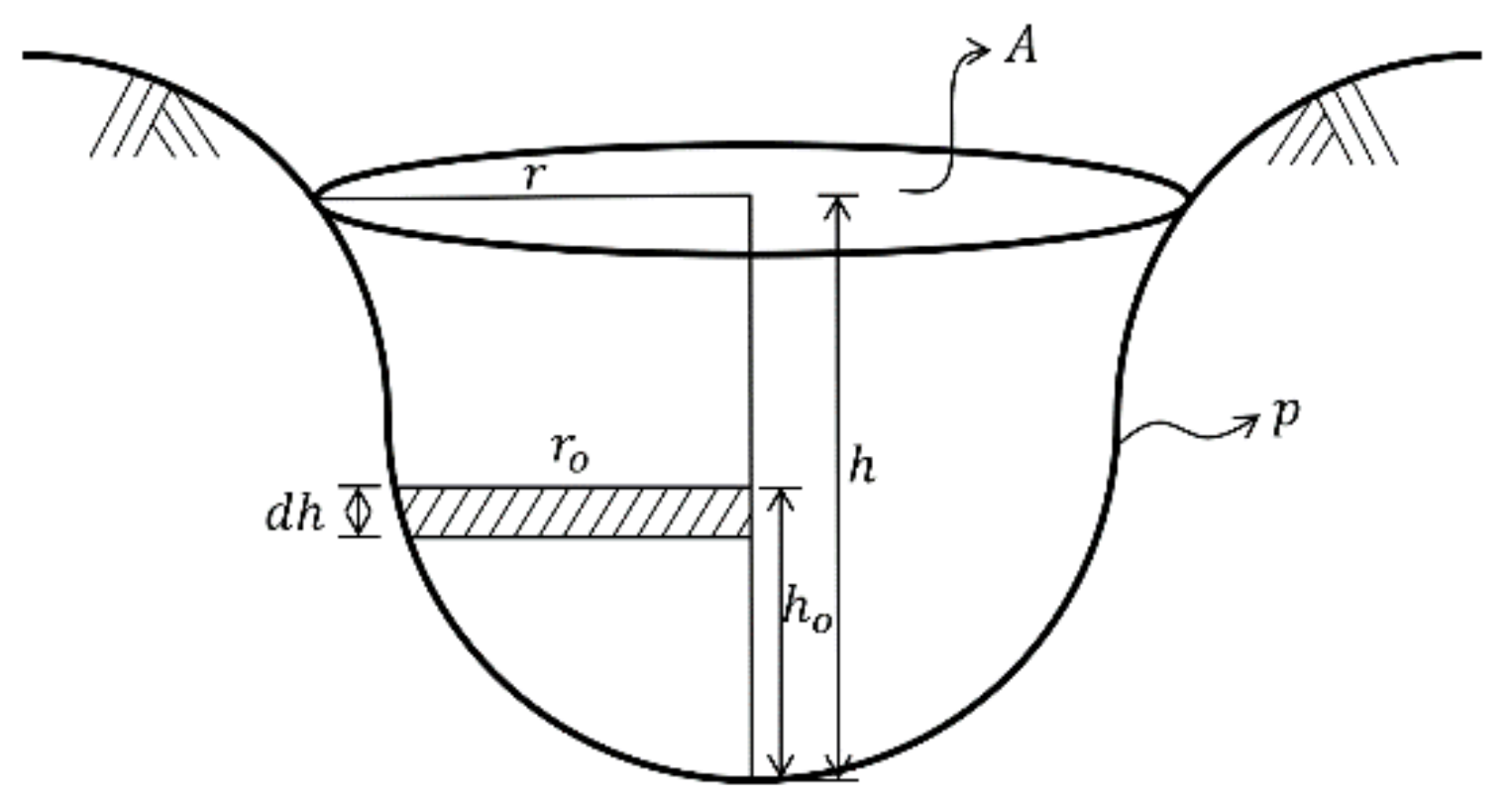
The geometry of a reservoir (Figure 2) is very important to identify the HC of the reservoir using the volume (V)-area (A)-depth (H) relationship. However, reservoirs differ in geometry, and therefore it is not possible to accurately express the geometry of a reservoir with a cross-section. In this study, it was assumed that the A-h and V-h relationships could be expressed using inverse functions. In addition, a basic mathematical theory was developed based on previous studies to derive first-order equations for these relationships. Thus, it was inferred that the A-h and V-h relationships were interdependent. Based on this, the following equations were derived [20,22].
The reservoir volume was obtained by integrating the area along the water depth, as shown in Equation (1).
where is an arbitrary variable for water depth, is the volume of the reservoir, is the water depth from the lowest point of the reservoir to the water surface, is the water depth to the infinitesimal area of the reservoir, and is the wetland surface area. It was assumed that was flat and was obtained by considering the wetland slope between dh, which is expressed as Equation (2).
where is the altitude of the ground surface corresponding to h, is the unit altitude of the ground surface, is the radius of the wetland, is the radius of an arbitrary infinitesimal area of the wetland, and is the shape factor of the side slope of the wetland. Because the area obtained using conventional methods, without considering the slope of the reservoir is , the change in area when factoring in water depth is and . Therefore, Equation (3) is expressed as .
In addition, the relationship of is derived from Equations (2) and (3), and Equation (4) is inferred.
Using Equation (4), the area is expressed as shown in Equation (5):
Therefore, the change in area with regards the slope is expressed by Equation (6).
The volume that factors in the shape of the sloped cross-section of the reservoir is expressed in Equation (7).
Using obtained from Equations (6) and (7), Equation (8) is derived.
2.3. Morphology Index and Equations for the Relationships between Basic Properties
2.3.1. Morphology Index
The morphology index of the reservoir was quantified using the average depth and full water area of the reservoir. According to Leonard and Crouzet [25], a morphology index of 10.5 or higher is considered a deep lake while a morphology index of 0.6 to 10.4 is considered a normal lake. A morphology index of 0.5 or less is classified as a shallow lake. Equation (9) shows the morphology index applied to reservoirs.
2.3.2. Full Water Storage Area-Levee Height Relationship
Lehner et al. [26] estimated the storage area of the full water-levee height relationship for reservoirs and lakes worldwide, as shown in Equation (10), and showed that the storage was approximately 29% (=1/3.42) of the product of the full water area and the levee height.
2.3.3. Full Water Storage Area Relationship
Takeuchi [24] estimated the full water storage area relationship for reservoirs worldwide with a full water area of 36.1 or high and a storage of 0.5 or higher as shown in Equation (11).
2.4. Cluster Analysis
Cluster analysis is a method for classifying data with similar characteristics into groups based on the characteristics of multiple subjects. This method is divided into hierarchical and non-hierarchical cluster analysis [23,32,33]. A representative method for hierarchical cluster analysis uses the distance between data points, such as the shortest and longest connections. A representative method for nonhierarchical cluster analysis is k-means clustering. The K-means cluster analysis classifies data with similar characteristics into K groups. This method groups data that are a short distance from a central point, providing the average data in each cluster. In this study, K-means cluster analysis was conducted to determine the optimal clusters by minimizing the distances between the data in each cluster and the central point; the cluster analysis process was terminated when the arbitrarily defined central point of each cluster could no longer minimize the error. Figure 3 illustrates the concept of cluster analysis.
3. Results
3.1. Data Description
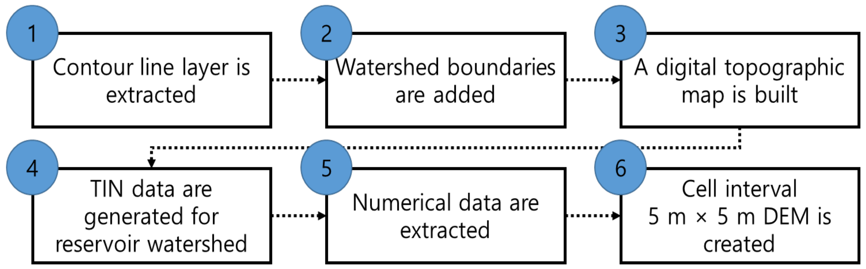
Models of the reservoirs were based on digital topographic maps (1:25,000) of Miryang City, Gyeongsangnam Province, which were provided by the National Spatial Information Portal. Procedures (1)–(6), as shown in Figure 4, were executed to quantitatively identify the altitude and topographic characteristics of the reservoirs. These procedures included: (1) contour line layer extraction, (2) the addition of watershed boundaries, (3) construction of a digital topographic map for each reservoir watershed, (4) generation of TIN data for each watershed, (5) numerical data extraction, and (6) the creation of a 5 × 5 m cell interval for each reservoir watershed. Topographic information was constructed for the ten reservoirs using topographic maps and GIS techniques, and the location and area by water depth were modeled for each reservoir (Figure 5).
3.2. Estimation of the Area-Volume Relationship of a Reservoir According to the Water Depth
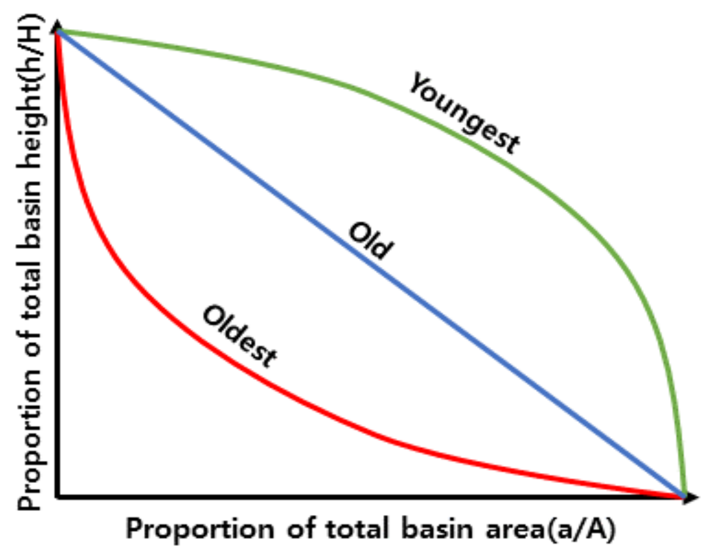
In this study, the application of HCs to reservoirs was attempted. HCs are divided into youthful, mature, and old stages (Figure 6). The youthful stage has the characteristics of a basin in which the original ground surface is not significantly eroded. The mature stage has the characteristics of a basin in which the ground surface is significantly eroded. The old stage has characteristics close to those of a peneplain because the ground surface is substantially eroded. In other words, for reservoirs, the old stage exhibits the highest level of erosion, followed by the mature and youthful stages [34]. Erosion causes reservoirs to have insufficient allowable storage capacity because the accumulated sediment in the reservoirs reduces the flood control capacity and may lead to their collapse during heavy rainfall events.
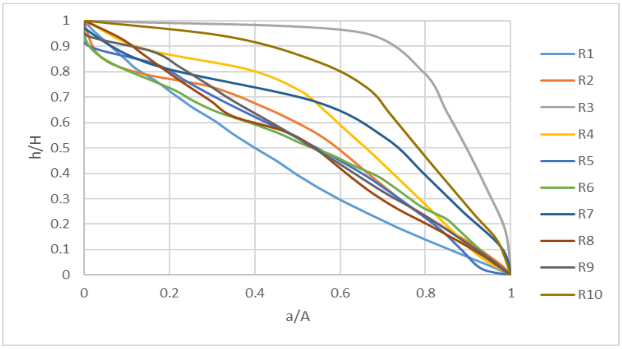
A HC according to the relative height (h/H) and relative area (a/A), was determined for each reservoir based on the topographic information constructed using topographic maps and GIS technique. The HC of a reservoir was created by calculating the area by elevation, and then connecting the altitude of the reservoir above sea level to the cumulative area above a certain altitude. In this instance, the Y-axis was defined as the ratio of a certain height (h) to the total height of the reservoir watershed (H), and the X-axis as the ratio of the cumulative area (a) above a certain height (h) to the total area of the reservoir watershed (A). Thus, the relative height was reflected by h/H and the relative area by a/A. Because h/H and a/A are relative values for each reservoir watershed, the volume and area for each reservoir were calculated as h increased from zero in 0.5 m increments. Table 1, Table 2, Table 3 and Table 4 show the area and volume according to the change in h for each reservoir.
A comparison with the reservoir volumes measured using unmanned water depth measuring equipment by the National Disaster Management Research Institute revealed that the error rate ranged from 0.23% to 14.27%, and the average error rate was 5.03% (Table 5). In addition, a HC was created for each reservoir using the a/A and h/H ratios (Figure 7).
3.3. Analysis of the Morphological Characteristics of the Reservoirs
To identify the characteristics of the reservoirs, the morphology index and full water storage area-levee height relationship used by Leonard and Crouzet (1999) and Lehner et al. (2004) were used. Leonard and Crouzet (1999) quantified the morphology index of a reservoir using the average depth and area of the reservoir at full water. In this study, the average morphology index of the ten reservoirs was found to be approximately 4.36; thus, they were classified as normal lakes. The R3, R4, R5, R7, R8, R9, and R10 reservoirs exhibited low morphology index values, indicating that they had lower depths than other reservoirs. In addition, the morphology index results revealed that reservoirs R1, R2, and R6 were deep lakes.
Lehner et al. (2004) proposed a relationship between reservoirs and lakes. In this study, the storage area of the full water-levee height relationship for the reservoirs was analyzed. Furthermore, the relationship between the storage, and the product of the area at full water and levee height was derived as shown in Equation (12).
The analysis results revealed that the R3, R4, R5, R7, R8, R9, and R10 reservoirs had a smaller area at full water relative to that of the R1, R2, and R6 reservoirs.
Takeuchi (1997) estimated the relationship between the full water area and the reservoir storage worldwide with a full water area of 36.1 or higher and a storage of 0.5 or higher. In this study, the relationship was analyzed for reservoirs in Korea, and Equation (13) was derived.
The results of the full water storage area relationship revealed that the R3, R4, R5, R7, R8, R9, and R10 reservoirs had a smaller storage relative to that of the R1, R2, and R6 reservoirs (Table 6).
3.4. Analysis of Reservoir Characteristics through Cluster Analysis
Cluster analysis was conducted, using the basic properties of each reservoir, to identify the reservoir characteristics with different properties. As shown in Table 7, the properties of the ten reservoirs were used as input data. The input data included the basin area, useful capacity, full water area, levee height, levee length, permissible area, irrigated area, and drought frequency.
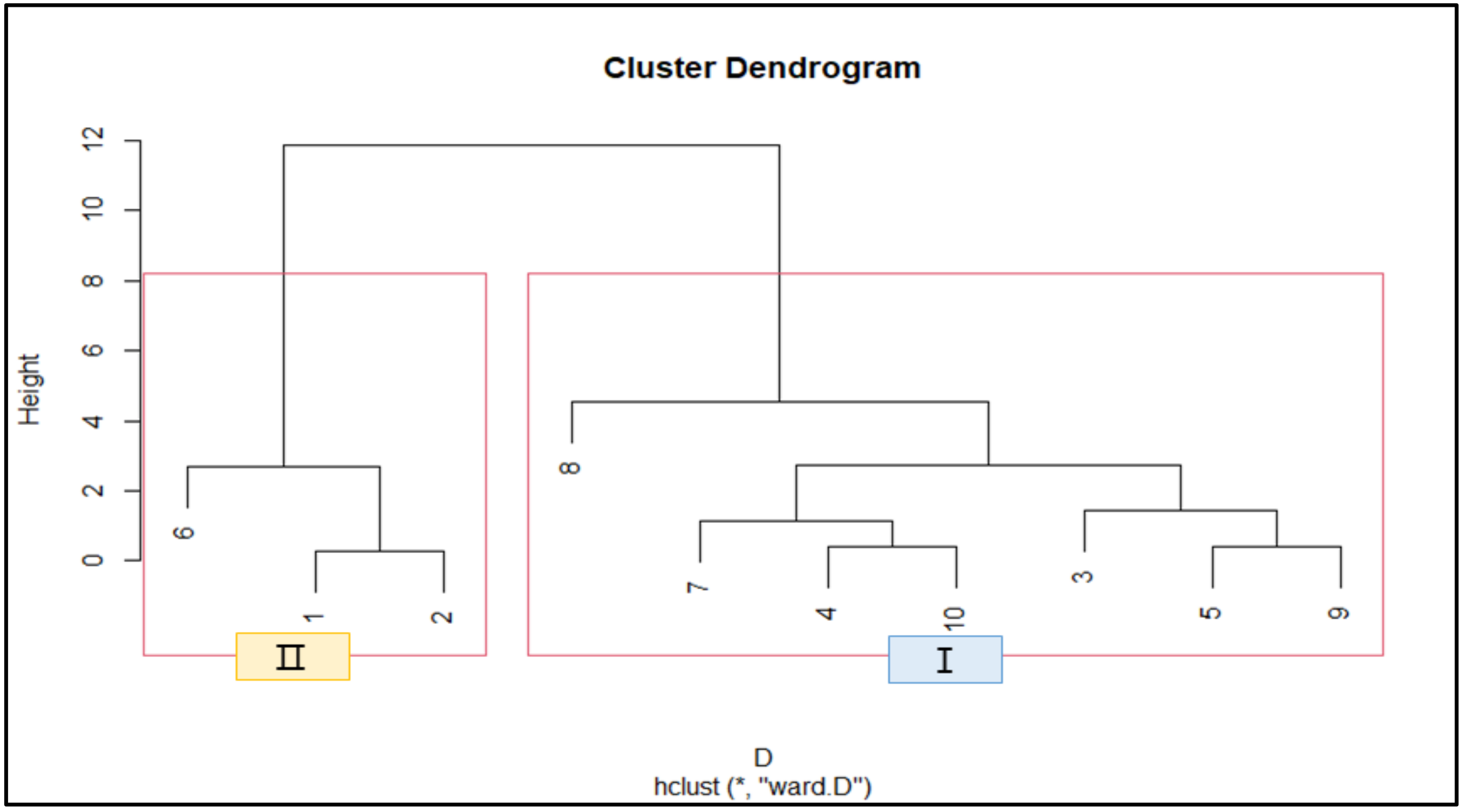
As shown in Figure 8, the cluster analysis classified the reservoirs into two groups: group (I) consisted of reservoirs R1, R2, and R6, whose useful capacity and full water area were large, and group (II) consisted of reservoirs R3, R4, R5, R7, R8, R9, and R10, whose useful capacity and full water area were small. The cluster analysis results, using the basic reservoir properties, revealed that the reservoirs could be classified based on their useful capacity and full water area; these indicators were identified as being more influential than other basic properties in the cluster analysis process.
3.5. Morphological Analysis of the Collapsed Reservoirs Using Cluster Analysis and HC
HCs and the cluster analysis method were applied to reservoirs that had collapsed and caused damage. Only recent cases located near Miryang City, Gyeongsangnam Province were investigated. The Sandae Reservoir, located in Gyeongju City, Gyeongsangbuk Province, collapsed in 2013 and had a full water area of 49,200 , a useful capacity of 194,400 , a levee height of 12.2 m, and a levee length of 210 m. The Goeyeon Reservoir, located in Yeongcheon City, Gyeongsangbuk Province, collapsed in 2014 and had a full water area of 61,000 , a useful capacity of 61,420 , a levee height of 5.5 m, and a levee length of 160 m. In this study, HCs and a cluster analysis were applied to the Sandae and Goeyeon reservoirs, which are located near the ten reservoirs and had caused damage in the past.
The morphology indexes were found to be 11.65 and 26.68 for the Sandae and Goeyeon reservoirs, respectively. These high morphology index values indicated that the reservoirs were deeper than other reservoirs. The results of the full water storage area-levee height relationship were found to be 1.13 and 2.26 for the Sandae and Goeyeon reservoirs, respectively, indicating that they had larger full water areas than other reservoirs. The results of the full water storage area relationships were 6.15 and 8.87 for the Sandae and Goeyeon reservoirs, respectively, indicating that they had a larger storage capacity than other reservoirs.
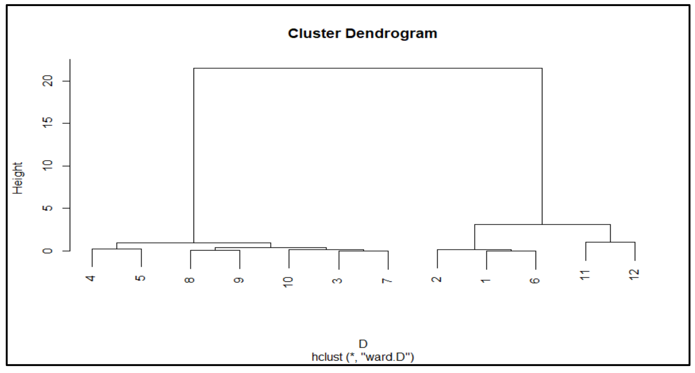
Cluster analysis was conducted using the properties of the ten reservoirs, as well as the Sandae (11) and Goeyeon (12) reservoirs, as input data. Cluster analysis classified the reservoirs into three groups: Group (I) included the R3, R4, R5, R7, R8, R9, and R10 reservoirs, whose full water area and useful capacity were relatively small, Group (II) included the R1, R2, and R6 reservoirs, whose full water area and useful capacity were relatively large, and Group (III) including the Sandae (11) and Goeyeon Reservoirs, whose full water area and useful capacity were the largest (Figure 9).
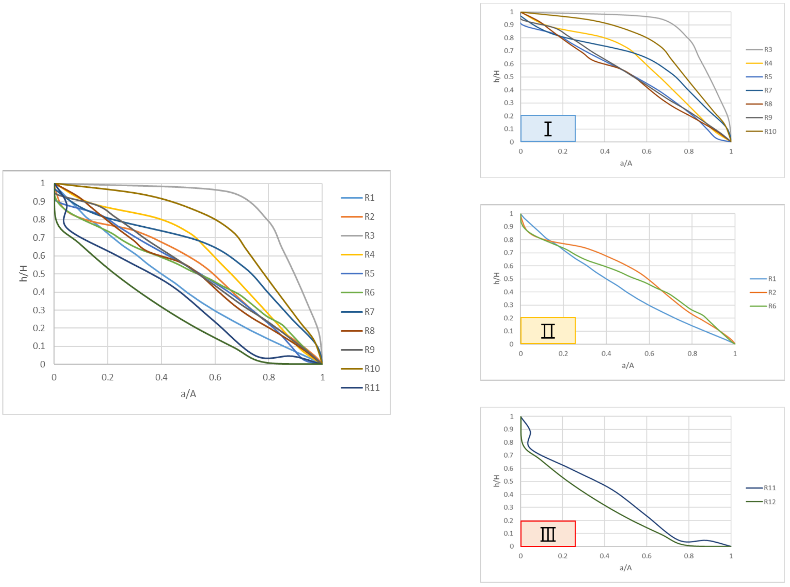
To identify the characteristics of each group, the morphological characteristics of the reservoirs were investigated using the HCs. It was found that group (I) had the original ground surface that was not significantly eroded, group (II) had the original ground surface that was significantly eroded, and group (III) had the original ground surface eroded more extensively (Figure 10).
The Sandae and Goeyeon reservoirs that collapsed had larger storage areas than the other reservoirs, and the HC results showed that considerable erosion occurred in their watersheds. In other words, the Sandae and Goeyeon reservoirs had insufficient allowable storage capacities compared to the other reservoirs.
4. Discussions and Conclusions
In this study, the geometry of unmeasured reservoirs was determined using topographic information, and a morphological analysis was conducted. The geometry and area by elevation and storage capacity of the reservoirs were determined by creating HCs for the reservoirs. In addition, the morphology index was quantitatively determined through an analysis of the full water storage area relationship for each reservoir. Topographic and morphological analyses of two reservoirs that had collapsed because of aging, insufficient management, and flooding were investigated to identify the potential causes of these collapses.
The area by elevation and volume for ten reservoirs located in Miryang City, Gyeongsangnam Province, including the Ga-Gog reservoir, were calculated using digital topographic maps. When the results were compared with the reservoir volumes measured by the National Disaster Management Research Institute, the error rate ranged from 0.23% to 14.27%. This error rate, with an average of approximately 5.03%, was excellent.
The full water storage area-levee height relationship and full water storage area relationship were comprehensively examined. It was found that the R3, R4, R5, R7, R8, R9, and R10 reservoirs had a lower depth and a smaller full water area relative to that of the R1, R2, and R6 reservoirs.
Cluster analysis was conducted to classify similar types of reservoirs into groups using basic properties, such as basin area, useful capacity, and full water area. The cluster analysis classified the reservoirs into two groups: the R1, R2, and R6 reservoirs, whose useful capacity and full water area were large, and the R3, R4, R5, R7, R8, R9, and R10 reservoirs, whose useful capacity and full water area were small. The useful capacity and full water area were identified as the indicators having the largest impact on the cluster analysis results.
HCs and the cluster analysis method were applied to two reservoirs that had collapsed and caused damage. The cluster analysis classified these two reservoirs and the ten reservoirs into three groups. The HCs of the collapsed reservoirs exhibited a convex downward shape compared to those of the other normal reservoirs, indicating that they were significantly aged and had been subjected to considerable erosion.
Each reservoir had different basic properties, such as a full water area and storage capacity. Should reservoir geometry be understood and the common characteristics of similar reservoir types be classified and identified using morphological analysis and HCs, these could be used to reduce the damage caused by reservoir collapse. The identification of potential causes of reservoir collapse prior to the disaster, through proactive disaster management, could possibly reduce the damage.
Author Contributions
Conceptualization by D.K. and H.S.K.; formal analysis by D.K.; methodology by W.W. and H.L.; supervision by H.S.K. and J.K.; writing of original draft by D.K.; writing of review and editing by D.K. and J.K. All authors have read and agreed to the published version of the manuscript.
Funding
This research was supported by a grant(2018-MOIS31-009) from the Fundamental Technology Development Program for Extreme Disaster Response, funded by the Korean Ministry of Interior and Safety (MOIS).
Institutional Review Board Statement
Not applicable.
Informed Consent Statement
Not applicable.
Data Availability Statement
Not applicable.
Conflicts of Interest
The authors declare no conflict of interest.
References
- Groombridge, B.; Jenkins, M. Freshwater Biodiversity: A Preliminary Global Assessment; WCMC Biodiversity Series Number 8; World Conservation Press: Cambridge, UK, 1998. [Google Scholar]
- Mitsch, W.J.; Gosselink, J.G. Wetlands, 3rd ed.; Wiley: New York, NY, USA, 2000. [Google Scholar]
- Revenga, C.; Brunner, J.; Henninger, N.; Kassem, K.; Payne, R. Pilot Analysis of Global Ecosystems (PAGE): Freshwater Systems; World Resources Institute (WRI): Washington, DC, USA, 2000. [Google Scholar]
- Sanderson, M.G. Global Distribution of Freshwater Wetlands for Use in STOCHEM; Technical Note 32 (HTCN 32); Hadley Centre for Climate Prediction and Research, Met Office: Bracknell, UK, 2001.
- Wetzel, R.G. Limnology: Lake and River Ecosystems, 3rd ed.; Academic Press: San Diego, CA, USA, 2001. [Google Scholar]
- Kim, D.H.; Kim, J.S.; Choi, C.H.; Wang, W.J.; You, Y.H.; Kim, H.S. Estimations of Hazard-Triggering Rainfall and Breach Discharge of Aging Reservoir. J. Korean Soc. Hazard Mitig. 2019, 19, 421–432. [Google Scholar] [CrossRef] [Green Version]
- National Disaster Management Research Institute. Annual Report. 2019. Available online: https://nidm.gov.in/PDF/pubs/AR2020.pdf (accessed on 15 November 2021).
- Kim, D.H.; Kim, J.S.; Wang, W.J.; Lee, J.S.; Jung, J.W.; Kim, H.S. Analysis of Morphological Characteristics of Collapsed Reservoirs in Korea. J. Korean Soc. Hazard Mitig. 2020, 20, 207–216. [Google Scholar] [CrossRef]
- Hong, B.M. Problems and improvement plans for the construction of agricultural reservoirs. Water Future 2004, 37, 29–33. [Google Scholar]
- Yoo, C.S.; Park, H.K. Analysis of Morphological Characteristics of Farm Dams in Korea. J. Korean Geogr. Soc. 2007, 42, 940–954. [Google Scholar]
- Graf, W.L. Dam nation: A geographic census of American dams and their large-scale hydrologic impacts. Water Resour. Res. 1999, 35, 1305–1311. [Google Scholar] [CrossRef]
- McDonald, C.P.; Rover, J.A.; Stets, E.G.; Striegl, R.G. The regional abundance and size distribution of lakes and reservoirs in the United States and implications for estimates of global lake extent. Limnol. Oceanogr. 2012, 57, 597–606. [Google Scholar] [CrossRef]
- Chang, Y.K.; Park, J.Y.; Moon, D.Y.; Kang, I.J. Calculation of Reservoir Capacity by Combination of GPS and Echo Sounder. J. Korean Soc. Geospat. Inf. Sci. 2002, 10, 27–35. [Google Scholar]
- Park, S.K.; Jeong, J.H. Calculation of Sediment Volume of the Agriculture Reservoir Using DGPS Echo-Sounder. J. GIS Assoc. Korea 2005, 13, 297–307. [Google Scholar]
- Choi, B.G.; Lee, H.S. Measuring Water Volume of Reservoir by Echosounding. J. Korea Soc. Geospat. Inf. Syst. 2007, 15, 55–59. [Google Scholar]
- Guerrero, M.; Lamberti, A. Flow Field and Morphology Mapping Using ADCP and Multibeam Techniques: Survey in the Po River. J. Hydraul. Eng. 2011, 137, 1576–1587. [Google Scholar] [CrossRef]
- Ilci, V.; Ozulu, I.M.; Alkan, R.M.; Erol, S.; Uysal, M. Determination of Reservoir Sedimentation with Bathymetric Survey: A Case Study of Obruk Dam Lake. J. Fresenius Environ. Bull. 2019, 28, 2305–2313. [Google Scholar]
- Song, B.G.; Oh, J.Y.; Kim, S.S.; Lee, T.W.; Park, K.H. Analysis of 3D Topographic Information on Reservoir Using UAV and Echo Sounder. J. Korean Soc. Hazard Mitig. 2018, 18, 563–568. [Google Scholar] [CrossRef] [Green Version]
- Langbein, W.B. Topographic Characteristics of Drainage Basin. U.S. Geolological Survey W.S. Paper 968-C. 1947. Available online: https://pubs.usgs.gov/wsp/0968c/report.pdf (accessed on 15 November 2021).
- Hayashi, M.; Kamp, G.V. Simple equations to represent the volume-area depth relations of shallow wetlands in small topographic depression. J. Hydrol. 2000, 237, 74–85. [Google Scholar] [CrossRef]
- Oertel, G.F. Hypsographic, hydro-hysographic and hydrological analysis of coastal bay environments, Great Machipongo Bay, Virginia. J. Coast. Res. 2001, 17, 775–783. [Google Scholar]
- Kim, J.G.; Kim, H.S.; Jeong, S.M. Estimation of Volume-Area-Depth Relationship for Shallow Wetland. J. Korea Water Resour. Assoc. 2002, 35, 231–240. [Google Scholar]
- Nam, W.H.; Kim, T.G.; Hong, E.M.; Hayes, M.J.; Svoboda, M.D. Water Supply Risk Assessment of Agricultural Reservoirs using Irrigation Vulnerability Model and Cluster Analysis. J. Korean Soc. Agric. Eng. 2015, 57, 59–67. [Google Scholar]
- Takeuchi, K. Least marginal environmental impact rule for reservoir development. Hydrol. Sci. J. 1997, 42, 583–597. [Google Scholar] [CrossRef] [Green Version]
- Leonard, J.; Crouzet, P. Lakes and Reservoir in the EEA Area; Topoc Report No. 1/1999; European Environment Agency (EEA): Copenhagen, Denmark, 1999. [Google Scholar]
- Lehner, B.; Doll, P. Development and validation of a global database of lakes, reservoir and wetlands. J. Hydrol. 2004, 296, 1–22. [Google Scholar] [CrossRef]
- Dargahi, B.; Setegn, S.G. Combined 3D hydrodynamic and watershed modelling of Lake Tana, Ethiopia. J. Hydrol. 2011, 398, 44–64. [Google Scholar] [CrossRef]
- Li, Y.; Zhang, Q.; Yao, J.; Werner, A.D.; Li, X. Hydrodynamic and hydrological modeling of the Poyang Lake catchment system in China. J. Hydrol. Eng. 2014, 19, 607–616. [Google Scholar] [CrossRef]
- Zhang, L.; Lu, J.; Chen, X.; Liang, D.; Fu, X.; Sauvage, S.; Sanchez Perez, J.-M. Stream flow simulation and verification in ungauged zones by coupling hydrological and hydrodynamic models: A case study of the Poyang Lake ungauged zone. Hydrol. Earth Syst. Sci. 2017, 21, 5847–5861. [Google Scholar] [CrossRef] [Green Version]
- Lopes, V.A.R.; Fan, F.M.; Pontes, P.R.M.; Siqueira, V.A.; Collischonn, W.; da Motta Marques, D. A first integrated modelling of a river-lagoon large-scale hydrological system for forecasting purposes. J. Hydrol. 2018, 565, 177–196. [Google Scholar] [CrossRef]
- Munar, A.M.; Cavalcanti, J.R.; Bravo, J.M.; Fan, F.M.; da Motta-Marques, D.; Fragoso, C.R. Coupling large-scale hydrological and hydrodynamic modeling: Toward a better comprehension of watershed-shallow lake processes. J. Hydrol. 2018, 564, 424–441. [Google Scholar] [CrossRef]
- Kyoung, M.S.; Kim, S.D.; Kim, B.K.; Kim, H.S. Construction of hydrological drought severity-area-duration curves using cluster analysis. J. Korean Soc. Civ. Eng. 2007, 27, 267–276. [Google Scholar]
- Han, S.M.; Hwang, G.S.; Choe, S.Y.; Park, J.W. A study on classifying algorithm of disaster recovery resources using statistical method. J. Korean Soc. Hazard Mitig. 2014, 14, 49–58. [Google Scholar] [CrossRef] [Green Version]
- Sarp, G.; Duzgun, S.; Toprak, V. Hypsometric properties of the hydrolic basins located on western part of NAFZ. In Proceedings of the 34th International Symposium on Remote Sensing of Environment, The GEOSS Era: Towards Operational Environmental Monitoring, Sydney, Australia, 10–15 April 2011. [Google Scholar]
Figure 1.
Study area and locations of 10 reservoirs including the Ga-Gog reservoir in Miryang city, Gyeongsangnam province.
Figure 1.
Study area and locations of 10 reservoirs including the Ga-Gog reservoir in Miryang city, Gyeongsangnam province.

Figure 2.
The Structure of a reservoir.

Figure 3.
Concept of cluster analysis.

Figure 4.
Reservoir modeling flow chart. To quantitatively identify the altitude and topographic characteristics of the reservoirs, procedures (1)–(6) were performed.
Figure 4.
Reservoir modeling flow chart. To quantitatively identify the altitude and topographic characteristics of the reservoirs, procedures (1)–(6) were performed.

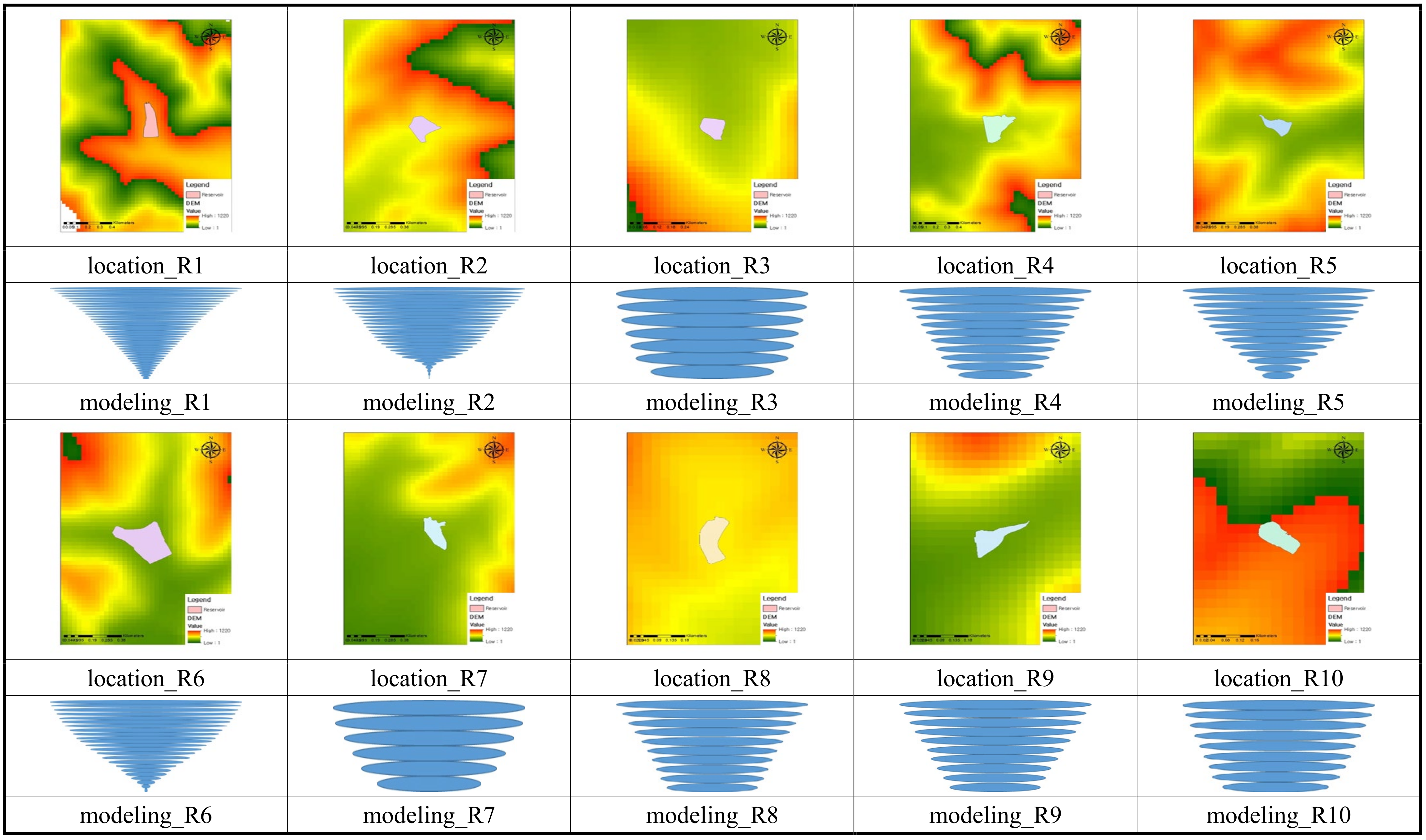
Figure 5.
Locations and modelling of the reservoirs: For the ten reservoirs, including the Ga-Gog Reservoir, topographic information was constructed using topographical maps and GIS techniques. Also, the location and the area in water depth were modeled for each reservoir.
Figure 5.
Locations and modelling of the reservoirs: For the ten reservoirs, including the Ga-Gog Reservoir, topographic information was constructed using topographical maps and GIS techniques. Also, the location and the area in water depth were modeled for each reservoir.

Figure 6.
Interpretation of Hypsometric Curve. HC is divided into the youthful, mature, and old stages.
Figure 6.
Interpretation of Hypsometric Curve. HC is divided into the youthful, mature, and old stages.

Figure 7.
Hypsometric curves for ten reservoirs created using the A-h and V-h relationship curves.

Figure 8.
Result of reservoir characteristics through cluster analysis.

Figure 9.
Result of the collapsed reservoirs using cluster analysis.

Figure 10.
Morphological analysis of the collapsed reservoirs using cluster analysis and HC.


Table 1.
Area measurements according to the change in reservoir height.
| h(m) | R1 | R2 | R3 | R4 | R5 | R6 | R7 | R8 | R9 | R10 |
|---|---|---|---|---|---|---|---|---|---|---|
| 0 | 0 | 0 | 0 | 0 | 0 | 0 | 0 | 0 | 0 | 0 |
| 0.5 | 1012 | 59 | 4033 | 1488 | 107 | 7 | 18 | 1073 | 53 | 4299 |
| 1.0 | 1542 | 227 | 5000 | 4177 | 2554 | 151 | 3385 | 1704 | 1467 | 6950 |
| 1.5 | 2088 | 433 | 5350 | 5510 | 3767 | 1060 | 11,230 | 2330 | 2071 | 8360 |
| 2.0 | 2634 | 809 | 5670 | 6180 | 5020 | 3053 | 14,660 | 2984 | 2628 | 9020 |
| 2.5 | 3164 | 1646 | 5960 | 6760 | 6390 | 6310 | 16,560 | 3679 | 3151 | 9640 |
| 3.0 | 3694 | 3402 | 6220 | 7360 | 7770 | 10,370 | 18,380 | 4332 | 3752 | 10,270 |
| 3.5 | 4477 | 6260 | 6300 | 7920 | 9030 | 14,330 | 20,290 | 5880 | 4354 | 10,910 |
| 4.0 | 5260 | 7870 | 8480 | 10,200 | 17,230 | 20,760 | 6690 | 4910 | 11,550 | |
| 4.5 | 5905 | 9080 | 9030 | 11,190 | 20,840 | 7270 | 5480 | 12,210 | ||
| 5.0 | 6550 | 10,230 | 9580 | 12,130 | 25,910 | 7830 | 6010 | 12,590 | ||
| 5.5 | 7235 | 11,250 | 10,150 | 12,990 | 30,470 | 8440 | 6560 | |||
| 6.0 | 7920 | 12,180 | 10,970 | 13,690 | 34,170 | 9170 | 7180 | |||
| 6.5 | 8720 | 12,950 | 14,410 | 38,610 | 10,050 | 7730 | ||||
| 7.0 | 9520 | 13,600 | 15,470 | 42,050 | 10,880 | 8240 | ||||
| 7.5 | 10,190 | 14,210 | 45,860 | 11,650 | 8760 | |||||
| 8.0 | 10,860 | 14,810 | 48,400 | 12,460 | 9230 | |||||
| 8.5 | 11,620 | 15,410 | 50,700 | |||||||
| 9.0 | 12,380 | 16,040 | 53,100 | |||||||
| 9.5 | 13,190 | 16,670 | 56,600 | |||||||
| 10.0 | 14,000 | 17,340 | 58,500 | |||||||
| 10.5 | 14,705 | 18,110 | 60,300 | |||||||
| 11.0 | 15,410 | 19,030 | 62,100 | |||||||
| 11.5 | 16,195 | 19,890 | 64,000 | |||||||
| 12.0 | 16,980 | 20,700 | 65,900 | |||||||
| 12.5 | 17,860 | 21,420 | 66,800 | |||||||
| 13.0 | 18,740 | 22,090 | ||||||||
| 13.5 | 19,720 | 22,530 | ||||||||
| 14.0 | 20,700 | |||||||||
| 14.5 | 21,715 | |||||||||
| 15.0 | 22,730 | |||||||||
| 15.5 | 23,845 | |||||||||
| 16.0 | 24,960 | |||||||||
| 16.5 | 26,135 | |||||||||
| 17.0 | 27,310 | |||||||||
| 17.5 | 28,510 | |||||||||
| 18.0 | 29,710 | |||||||||
| 18.5 | 31,070 | |||||||||
Table 2.
Area estimations according to the change in reservoir height.
| h(m) | R1 | R2 | R3 | R4 | R5 | R6 | R7 | R8 | R9 | R10 |
|---|---|---|---|---|---|---|---|---|---|---|
| 0 | 0 | 0 | 0 | 0 | 0 | 0 | 0 | 0 | 0 | 0 |
| 0.5 | 1012 | 59 | 4029 | 1484 | 107 | 7 | 18 | 1030 | 53 | 4084 |
| 1.0 | 1542 | 227 | 4995 | 4164 | 2549 | 151 | 3375 | 1635 | 1466 | 6603 |
| 1.5 | 2088 | 432 | 5345 | 5493 | 3759 | 1059 | 11,196 | 2236 | 2069 | 7942 |
| 2.0 | 2634 | 807 | 5664 | 6161 | 5010 | 3050 | 14,616 | 2864 | 2625 | 8569 |
| 2.5 | 3164 | 1643 | 5954 | 6740 | 6377 | 6304 | 16,510 | 3531 | 3148 | 9158 |
| 3.0 | 3694 | 3395 | 6214 | 7338 | 7754 | 10,360 | 18,325 | 4158 | 3748 | 9757 |
| 3.5 | 4477 | 6247 | 6294 | 7896 | 9012 | 14,316 | 20,229 | 5644 | 4350 | 10,365 |
| 4.0 | 5260 | 7854 | 8455 | 10,180 | 17,213 | 20,698 | 6422 | 4905 | 10,973 | |
| 4.5 | 5905 | 9062 | 9003 | 11,168 | 20,819 | 6979 | 5475 | 11,600 | ||
| 5.0 | 6550 | 10,210 | 9551 | 12,106 | 25,884 | 7516 | 6004 | 11,961 | ||
| 5.5 | 7235 | 11,228 | 10,120 | 12,964 | 30,440 | 8102 | 6553 | |||
| 6.0 | 7920 | 12,156 | 10,937 | 13,663 | 34,136 | 8803 | 7173 | |||
| 6.5 | 8720 | 12,924 | 14,381 | 38,571 | 9648 | 7722 | ||||
| 7.0 | 9520 | 13,573 | 15,439 | 42,008 | 10,444 | 8232 | ||||
| 7.5 | 10,190 | 14,182 | 45,814 | 11,184 | 8751 | |||||
| 8.0 | 10,860 | 14,780 | 48,352 | 11,961 | 9221 | |||||
| 8.5 | 11,620 | 15,379 | 50,649 | |||||||
| 9.0 | 12,380 | 16,008 | 53,047 | |||||||
| 9.5 | 13,190 | 16,637 | 56,543 | |||||||
| 10.0 | 14,000 | 17,305 | 58,442 | |||||||
| 10.5 | 14,705 | 18,074 | 60,240 | |||||||
| 11.0 | 15,410 | 18,992 | 62,038 | |||||||
| 11.5 | 16,195 | 19,850 | 63,936 | |||||||
| 12.0 | 16,980 | 20,659 | 65,834 | |||||||
| 12.5 | 17,860 | 21,377 | 66,733 | |||||||
| 13.0 | 18,740 | 22,046 | ||||||||
| 13.5 | 19,720 | 22,485 | ||||||||
| 14.0 | 20,700 | |||||||||
| 14.5 | 21,715 | |||||||||
| 15.0 | 22,730 | |||||||||
| 15.5 | 23,845 | |||||||||
| 16.0 | 24,960 | |||||||||
| 16.5 | 26,135 | |||||||||
| 17.0 | 27,310 | |||||||||
| 17.5 | 28,510 | |||||||||
| 18.0 | 29,710 | |||||||||
| 18.5 | 31,070 | |||||||||
Table 3.
Volume measurements according to the change in reservoir height.
| h(m) | R1 | R2 | R3 | R4 | R5 | R6 | R7 | R8 | R9 | R10 |
|---|---|---|---|---|---|---|---|---|---|---|
| 0 | 0 | 0 | 0 | 0 | 0 | 0 | 0 | 0 | 0 | 0 |
| 0.5 | 843 | 14 | 1109 | 342 | 9 | 1 | 3 | 333 | 14 | 1397 |
| 1.0 | 2081 | 139 | 4742 | 2719 | 891 | 51 | 1497 | 1555 | 790 | 6468 |
| 1.5 | 3866 | 485 | 8021 | 7072 | 3698 | 696 | 10,084 | 3268 | 2724 | 12,631 |
| 2.0 | 6209 | 1223 | 11,296 | 11,456 | 7337 | 3393 | 24,337 | 5633 | 4793 | 18,684 |
| 2.5 | 9074 | 3032 | 14,828 | 15,916 | 12,380 | 10,065 | 37,152 | 8729 | 7339 | 24,725 |
| 3.0 | 12,447 | 7496 | 18,575 | 20,898 | 18,904 | 22,101 | 50,314 | 12,497 | 10,493 | 31,358 |
| 3.5 | 16,873 | 16,764 | 19,969 | 26,434 | 26,628 | 38,903 | 65,352 | 18,484 | 14,348 | 38,654 |
| 4.0 | 22,541 | 28,048 | 32,472 | 35,287 | 57,597 | 71,632 | 25,894 | 18,713 | 46,605 | |
| 4.5 | 28,638 | 37,883 | 39,047 | 44,598 | 78,995 | 32,248 | 23,585 | 55,242 | ||
| 5.0 | 35,061 | 47,985 | 46,153 | 54,452 | 108,694 | 38,656 | 28,955 | 61,628 | ||
| 5.5 | 42,251 | 58,748 | 53,863 | 64,935 | 145,179 | 45,719 | 34,819 | |||
| 6.0 | 50,239 | 69,939 | 64,733 | 75,638 | 182,608 | 53,887 | 41,495 | |||
| 6.5 | 59,322 | 81,296 | 86,689 | 223,799 | 63,618 | 48,756 | ||||
| 7.0 | 69,586 | 92,527 | 102,040 | 268,195 | 74,511 | 56,214 | ||||
| 7.5 | 80,121 | 103,870 | 314,278 | 85,839 | 64,090 | |||||
| 8.0 | 90,831 | 115,645 | 360,545 | 98,851 | 72,050 | |||||
| 8.5 | 102,621 | 127,982 | 403,833 | |||||||
| 9.0 | 115,560 | 141,053 | 448,935 | |||||||
| 9.5 | 129,512 | 154,882 | 501,878 | |||||||
| 10.0 | 144,515 | 169,540 | 555,358 | |||||||
| 10.5 | 159,743 | 185,581 | 602,910 | |||||||
| 11.0 | 175,119 | 203,713 | 651,780 | |||||||
| 11.5 | 191,684 | 223,206 | 703,008 | |||||||
| 12.0 | 209,500 | 242,931 | 756,668 | |||||||
| 12.5 | 228,725 | 262,618 | 791,556 | |||||||
| 13.0 | 249,429 | 282,162 | ||||||||
| 13.5 | 271,720 | 297,392 | ||||||||
| 14.0 | 295,672 | |||||||||
| 14.5 | 320,869 | |||||||||
| 15.0 | 347,338 | |||||||||
| 15.5 | 375,627 | |||||||||
| 16.0 | 405,814 | |||||||||
| 16.5 | 437,629 | |||||||||
| 17.0 | 471,118 | |||||||||
| 17.5 | 506,008 | |||||||||
| 18.0 | 542,319 | |||||||||
| 18.5 | 584,400 | |||||||||
Table 4.
Volume estimations according to the change in reservoir height.
| h(m) | R1 | R2 | R3 | R4 | R5 | R6 | R7 | R8 | R9 | R10 |
|---|---|---|---|---|---|---|---|---|---|---|
| 0 | 0 | 0 | 0 | 0 | 0 | 0 | 0 | 0 | 0 | 0 |
| 0.5 | 252 | 15 | 1007 | 371 | 27 | 2 | 4 | 258 | 13 | 1021 |
| 1.0 | 1273 | 143 | 4512 | 2824 | 1328 | 79 | 1696 | 1333 | 759 | 5343 |
| 1.5 | 2714 | 494 | 7755 | 7243 | 4731 | 907 | 10,928 | 2904 | 2651 | 10,908 |
| 2.0 | 4708 | 1240 | 11,009 | 11,655 | 8769 | 4109 | 25,812 | 5101 | 4694 | 16,511 |
| 2.5 | 7226 | 3063 | 14,523 | 16,126 | 14,234 | 11,692 | 38,908 | 7996 | 7217 | 22,159 |
| 3.0 | 10,256 | 7557 | 18,252 | 21,116 | 21,198 | 24,995 | 52,253 | 11,536 | 10,344 | 28,372 |
| 3.5 | 14,256 | 16,875 | 21,888 | 26,660 | 29,341 | 43,182 | 67,469 | 17,156 | 14,171 | 35,212 |
| 4.0 | 19,416 | 28,203 | 32,702 | 38,383 | 63,057 | 81,854 | 24,134 | 18,509 | 42,674 | |
| 4.5 | 25,046 | 38,061 | 39,279 | 48,031 | 85,572 | 30,154 | 23,354 | 50,787 | ||
| 5.0 | 31,044 | 48,178 | 46,385 | 58,183 | 116,758 | 36,240 | 28,696 | 58,900 | ||
| 5.5 | 37,795 | 58,952 | 54,095 | 68,942 | 154,890 | 42,953 | 34,533 | |||
| 6.0 | 45,329 | 70,149 | 63,170 | 79,880 | 193,726 | 50,717 | 41,179 | |||
| 6.5 | 53,918 | 81,509 | 91,142 | 236,298 | 59,966 | 48,409 | ||||
| 7.0 | 63,648 | 92,739 | 104,371 | 282,028 | 70,325 | 55,839 | ||||
| 7.5 | 73,691 | 104,079 | 329,333 | 81,108 | 63,686 | |||||
| 8.0 | 83,947 | 115,848 | 376,663 | 92,582 | 71,888 | |||||
| 8.5 | 95,253 | 128,178 | 420,754 | |||||||
| 9.0 | 107,676 | 141,242 | 466,633 | |||||||
| 9.5 | 121,093 | 155,062 | 520,554 | |||||||
| 10.0 | 135,542 | 169,710 | 574,925 | |||||||
| 10.5 | 150,249 | 185,740 | 623,076 | |||||||
| 11.0 | 165,136 | 203,861 | 672,527 | |||||||
| 11.5 | 181,184 | 223,342 | 724,350 | |||||||
| 12.0 | 198,453 | 243,053 | 778,621 | |||||||
| 12.5 | 217,097 | 262,724 | 828,546 | |||||||
| 13.0 | 237,186 | 282,249 | ||||||||
| 13.5 | 258,826 | 300,583 | ||||||||
| 14.0 | 282,091 | |||||||||
| 14.5 | 306,586 | |||||||||
| 15.0 | 332,337 | |||||||||
| 15.5 | 359,873 | |||||||||
| 16.0 | 389,269 | |||||||||
| 16.5 | 420,269 | |||||||||
| 17.0 | 452,920 | |||||||||
| 17.5 | 486,960 | |||||||||
| 18.0 | 522,408 | |||||||||
| 18.5 | 560,528 | |||||||||
Table 5.
Reservoir volume comparison and results.
| Classification | Error Rate (Measurement Estimation) | Error Rate (Measurement Estimation) | ||
|---|---|---|---|---|
| R1 | 584,400 | 560,528 | 4.08% | 4.26% |
| R2 | 297,392 | 300,583 | −1.07% | −1.06% |
| R3 | 19,969 | 21,888 | 9.61% | −8.77% |
| R4 | 64,733 | 63,170 | 2.41% | 2.47% |
| R5 | 102,040 | 104,371 | −2.28% | −2.23% |
| R6 | 791,556 | 828,546 | −4.67% | −4.46% |
| R7 | 71,632 | 81,854 | −14.27% | −12.49% |
| R8 | 98,851 | 92,582 | 6.34% | 6.77% |
| R9 | 72,050 | 71,888 | 0.22% | 0.23% |
| R10 | 61,628 | 58,900 | 4.43% | 4.63% |
Table 6.
Analysis of the results of reservoir morphological characteristics.
| Classification | Value (Leonard, 1999) | Value (Lehner, 2004) | Value (Takeuchi, 1997) |
|---|---|---|---|
| R1 | 5.70 | 1.45 | 3.65 |
| R2 | 5.38 | 1.08 | 3.05 |
| R3 | 3.76 | 2.09 | 1.30 |
| R4 | 2.00 | 17.87 | 0.86 |
| R5 | 2.78 | 4.23 | 1.36 |
| R6 | 13.18 | 0.61 | 11.32 |
| R7 | 1.75 | 1.85 | 0.95 |
| R8 | 2.60 | 6.86 | 1.17 |
| R9 | 4.29 | 1.69 | 1.71 |
| R10 | 2.19 | 2.11 | 0.98 |
Table 7.
Basic properties of ten reservoirs.
| Classification | Basin Area (km2) | Useful Capacity (1000 m3) | Full Water Area (m2) | Levee Height (m) | Levee Length (m) | Permissible Area (ha) | Area Irrigated (ha) | Frequency of Drought (Year) |
|---|---|---|---|---|---|---|---|---|
| R1 | 1.5 | 480 | 31,070 | 12.5 | 84 | 35 | 28 | 1 |
| R2 | 0.5 | 280 | 22,530 | 6.2 | 172 | 8.7 | 8.7 | 10 |
| R3 | 0.6 | 28.9 | 6300 | 8.5 | 101 | 10 | 6 | 1 |
| R4 | 1.1 | 35.4 | 10,970 | 18 | 170 | 36.6 | 25 | 1 |
| R5 | 1.7 | 82.1 | 15,470 | 12.5 | 130 | 47 | 12 | 10 |
| R6 | 2.2 | 349 | 66,800 | 10 | 207 | 67.9 | 40.6 | 10 |
| R7 | 1.0 | 80 | 20,760 | 6.3 | 180 | 28.1 | 23.1 | 1 |
| R8 | 0.4 | 55.4 | 12,460 | 14.1 | 140 | 14 | 9 | 10 |
| R9 | 0.4 | 58.2 | 9230 | 10.2 | 112 | 10.4 | 8 | 10 |
| R10 | 0.6 | 47.3 | 12,590 | 7.6 | 241 | 42.2 | 15 | 1 |
Publisher’s Note: MDPI stays neutral with regard to jurisdictional claims in published maps and institutional affiliations. |
© 2022 by the authors. Licensee MDPI, Basel, Switzerland. This article is an open access article distributed under the terms and conditions of the Creative Commons Attribution (CC BY) license (https://creativecommons.org/licenses/by/4.0/).
Share and Cite
MDPI and ACS Style
Kim, D.; Kim, J.; Wang, W.; Lee, H.; Kim, H.S. On Hypsometric Curve and Morphological Analysis of the Collapsed Irrigation Reservoirs. Water 2022, 14, 907. https://doi.org/10.3390/w14060907
AMA Style
Kim D, Kim J, Wang W, Lee H, Kim HS. On Hypsometric Curve and Morphological Analysis of the Collapsed Irrigation Reservoirs. Water. 2022; 14(6):907. https://doi.org/10.3390/w14060907
Chicago/Turabian StyleKim, Donghyun, Jongsung Kim, Wonjoon Wang, Haneul Lee, and Hung Soo Kim. 2022. "On Hypsometric Curve and Morphological Analysis of the Collapsed Irrigation Reservoirs" Water 14, no. 6: 907. https://doi.org/10.3390/w14060907
Note that from the first issue of 2016, this journal uses article numbers instead of page numbers. See further details here.