
Hydrodynamic Characteristics at Intersection Areas of Ship and Bridge Pier with Skew Bridge
by
 ,
,
Anbin Li
1 ,
,
Genguang Zhang
1,*,
Xiaoping Liu
2,
Yuanhao Yu
1,
Ximin Zhang
1,
Huigang Ma
1 and
Jiaqiang Zhang
2 1
Key Laboratory of Agricultural Soil and Water Engineering in Arid and Semiarid Areas, Ministry of Education, Northwest A & F University, Weihui Road, Yangling 712100, China
2
School of Hydraulic Engineering, Changsha University of Science and Technology, Chiling Road, Changsha 410114, China
*
Author to whom correspondence should be addressed.
Water 2022, 14(6), 904; https://doi.org/10.3390/w14060904
Submission received: 20 February 2022
/
Revised: 9 March 2022
/
Accepted: 10 March 2022
/
Published: 14 March 2022
(This article belongs to the Section Hydraulics and Hydrodynamics)
Abstract
:Ships sailing in the area of a bridge are vulnerable to the influence of complex water flow, due to the complex flow pattern around the bridge pier. Ships often crash into bridge piers, leading to serious economic losses and threating personal safety. Based on the common forms of piers of skew bridges, the hydrodynamic problems encountered during ship–bridge interactions in the area of a skew bridge were studied using particle image velocimetry-based flume testing, physical model testing, and numerical simulation. The influence of the flow angle of attack of a round-ended pier on the force and center of gravity of a ship moving on both sides of a pier is discussed under various ship–bridge transverse spacings. The results show that as a ship passes through the bridge area, the bow roll moment exhibits three peak values: ‘positive’, ‘negative’, and ‘positive’, and the curve of the center of gravity position forms the shape of a ‘straw hat’. With an increase in the flow angle of attack of the pier, the negative peak value and the second positive peak value of the bow roll moment of the ship passing through the back flow side of the pier become greater than those on the upstream side. Moreover, the ship’s navigation attitude is more unstable compared to that upstream, and the ship is at risk of colliding with the pier and sweeping. The width of the restricted water area, determined by the hydrodynamic action between the ship and bridge in the skew bridge area, is the same as that determined by the critical lateral velocity. For the ship class referred to in this study, the current code can also be used in channel design, to safeguard ship and personal safety with piers with a large flow angle of attack.
1. Introduction
China has an extensive network of rivers, roads, and railways. Thousands of bridges have been built across rivers; however, piers have become obstacles to navigation. Navigation safety in the area of inland river bridges has become a concern. The piers built in inland river channels block the movement of incoming flow and create a complex 3D flow pattern [1] around them. Ships sailing in these areas are often subjected to turbulence around the piers, and the complex forces cause deflection and deviation, which is not conducive to safe navigation [2].
Due to the difficulty in measuring the flow around piers, scholars generally reduce the size of the measured pier based on a geometric scale, build a flume model in a laboratory to perform tests, or use numerical simulations to study the complex 3D flow structure around a pier. Most experimental studies on the flow around piers have been conducted considering the scouring of the pier. Many scholars [3,4,5,6,7,8,9] have conducted flume model tests on the flow around a pier, in which the back water, shock wave, horseshoe vortex at the pier side, trailing vortex at the pier side, vortex street off, and effects of pier geometry were analyzed. The influences of the water depth, velocity, pier type, and pier diameter on the 3D flow characteristics around piers have been studied. Al-saffar [10] found that the formation of a horseshoe vortex in front of a pier is strongly correlated to the Reynolds number, pier diameter, Froude number, and water depth. Chakrabarti and McBride [11] studied the flow structure between two piers with rapids and analyzed the stress acting on the pier, the velocity of the flow field around the pier, and vortex system structure. Vijayasree et al. [2] studied the difference in the flow field between a square column and a cylinder using a comparative test and showed that the turbulence of the water flow around the cylinder was greater than that around the square column. Daichin and Lee [12] used a single-frame particle image velocimetry (PIV) test to measure the flow field around an immersed elliptical cylinder with a ratio of two axes under the subcritical Reynolds number. The wake width of the elliptical cylinder was found to be smaller than that of the cylinder. Gautam et al. [13] used PIV to observe the flow field around a complex array column and found that the average flow velocity and turbulence parameters around the array column were lower than those around a single column. Carnacina [14] studied the average three-dimensional flow velocities, turbulence intensities, Reynolds stress, and turbulent kinetic energy for a cross-section corresponding to the center of the pier using a Nortek acoustic velocimeter. With the progress of computer technology, scholars have started using numerical models to predict the flow structure around piers. Currently, the large eddy simulation (LES) method and Reynolds-averaged Navier–Stokes (RANS) method are widely used for simulations, among which the latter is favored by engineering scholars, because it can perform efficient simulation, while ensuring accuracy. Salaheldin et al. [1], Paul et al. [15], and Shi et al. [16] obtained relatively realistic flow characteristics around a bluff body through a numerical simulation. Salaheldin et al. [1] used the k-ε turbulence model, based on RANS, to simulate the flow and scouring process around a circular pier. Paul et al. (2014) used a numerical model to simulate the flow field around an elliptical cylinder with different axial ratios under laminar flow conditions at different flow angles of attack. The authors found that the elliptical shape parameters and Reynolds number influenced the vortex shedding behavior. Shi et al. [16] simulated the flow field around an elliptical cylinder with an axial ratio range of 0.25–1.0 and a flow angle of attack range of 0–90° under a Reynolds number of 150; the flow pattern around the cylinder was divided into three types: steady wake, Kármán wake followed by a steady wake, and Kármán wake followed by a secondary wake.
Based on the flow structure around bridge piers, in recent years, some scholars have studied the movement of ships in navigable waters around bridge piers. Since there have been few systematic studies on flow patterns around round-ended piers with similar elliptical sections, under different flow angles of attack and subcritical flow or supercritical flow conditions, most current studies focus on the intersection between ships and circular piers. Zhang et al. [17] improved the method used by Tuck and Newman [18], to study the intersection of two ships. The bridge pier was considered a static ship, and the thin body theory and slender body theory were applied to study the change law of the flow structure during ship–bridge intersection and the hydrodynamic effect acting on the ship throughout the process. The force and moment of a ship passing through a bridge pier will peak at a certain moment; these are important parameters affecting the lateral drift and bow roll of the ship. Liu et al. [19] suggested that the spacing between ships and bridges is an important factor affecting the safety of ships. Based on previous studies, the influences of different spacings on the forces and moments of ships navigating in the area of a bridge have been discussed, by combining physical model tests and numerical simulations. Wang and Wang [20] found that ship motion can be simulated in a relatively accurate manner using the RNG k-ε model. Li et al. [21] used a numerical model to simulate the movement of a ship passing through the clearance between two parallel rectangular piers and found that the turbulence due to the piers had an important impact on ship safety. Based on the 3D N–S equation, Geng et al. [22] used a 3D numerical model to simulate the process of ships passing through an area with a circular bridge pier. The authors found that the movement of ships increased the transverse velocity in the area around the bridge pier, and that the ship size had a significant effect on the flow field.
China’s current navigable standard for inland rivers (GB50139-2014) 5.2.1 [23] proposes that the intersection angle between the normal direction of structures built across rivers and the flow direction of water should not exceed 5°, without giving detailed guidance for situations above 5°. Due to the high speed and large curvature radius of railways, particularly high-speed railways, the oblique angle between the bridge axis and the river cannot meet this requirement. Considering the structural safety of railway bridges, round-ended piers are commonly used. The current railway bridge and culvert design code (TB10002-2017) 3.1.7 [24] proposes that the bridge axis should be orthogonal to the pier axis and that the skew should not be less than 60° when avoidable. In this case, piers for high-speed railway bridges across rivers will inevitably have a certain amount of water flow angle of attack. The above study mainly discussed the process of ships moving past the side of a circular pier with a section, and there has been little discussion on circular piers with a water flow angle of attack.
It is important to study the complex flow field around round-ended piers under different flow angles of attack, in a bid to ensure the safety of ships passing through such bridge areas. Based on the common barge types in the Yangtze and Xiangjiang Rivers, and the common pier types of railway bridges, this study adopts PIV flume testing, ship–bridge intersection physical model testing, and numerical simulation to conduct relevant research.
2. Model Test
In this study, a model test on the flow around a pier and a physical model test on the ship–bridge intersection process were conducted. In the model test, the characteristics of the surface flow field under different flow angles of attack were studied. In the physical model test, the variation law of the bow roll moment during the intersection process was determined.
2.1. Model Test of Flow around a Round-Ended Pier
2.1.1. Flow Patterns and Fields around a Pier on a Fixed Bed
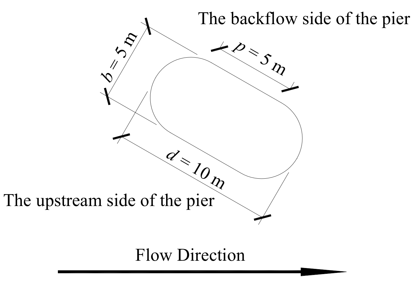
The flow around a round-ended pier of a skew bridge was the background for this study. Referring to the bridge pier type in the Yangtze and Xiangjiang Rivers, the section width of the round-ended pier was b = 5 m, the length was d = 10 m, and the internal rectangular side length was p = 5 m. The geometric scale of the model relative to the prototype was 1:200. Figure 1 shows a schematic of the shape of the bridge pier section. Based on the surface flow velocity of the Yangtze and Xiangjiang rivers in the navigable period, the river flow velocity was 2 m/s. On this basis, the flow regime was observed under flow angles of attack of α = 0°, 15°, 30°, and 45°.
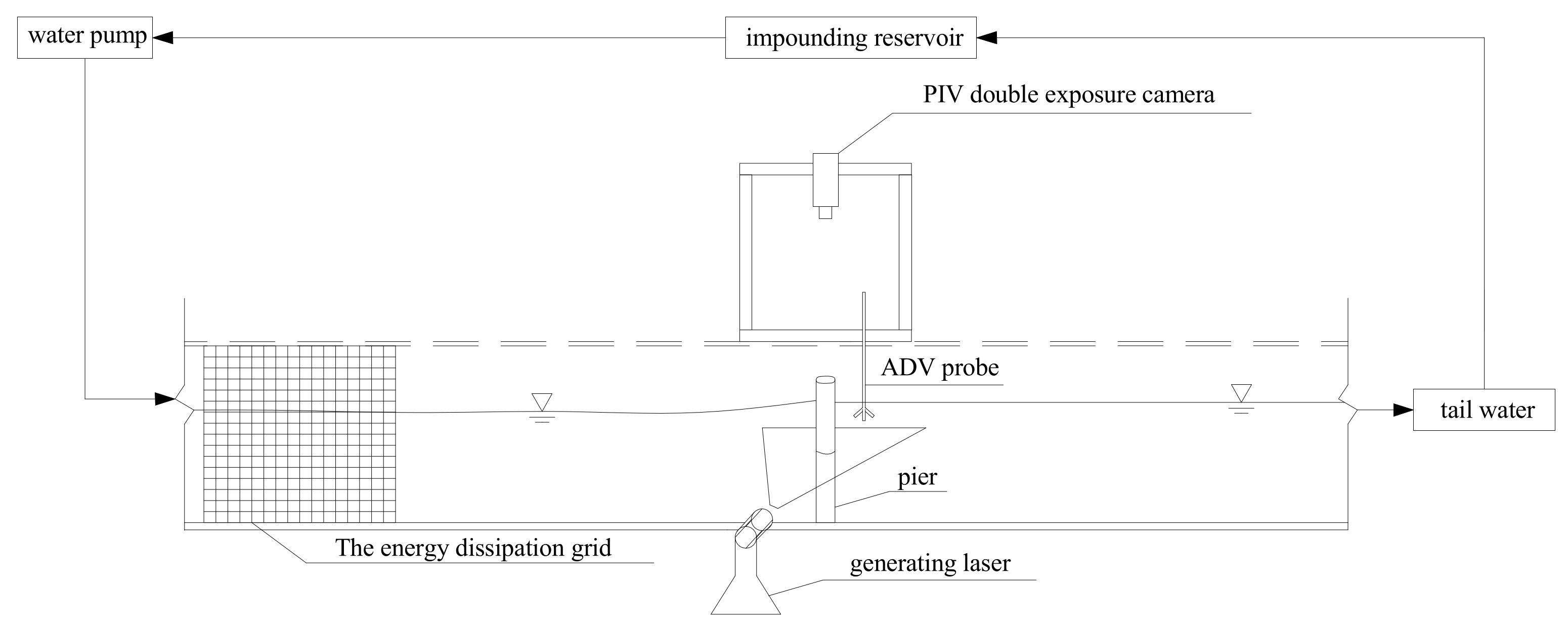
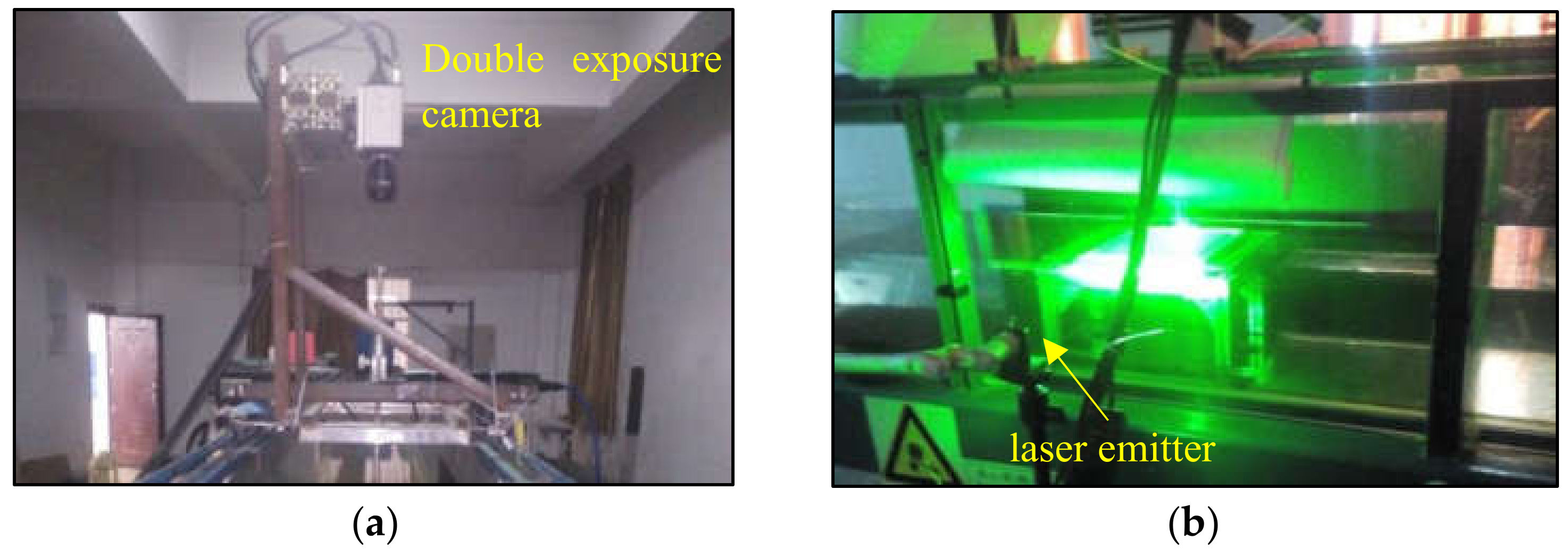
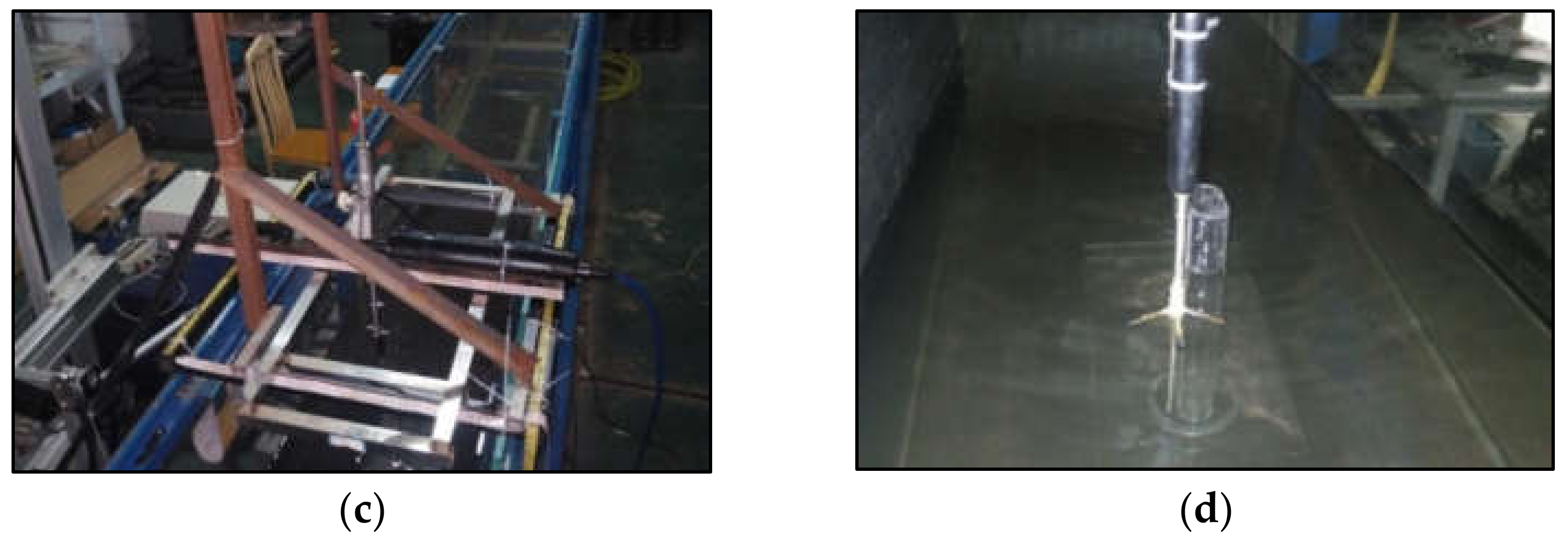
Physical model tests were conducted in a plexiglass tank in a PIV laboratory. The tank dimensions were 16, 0.4, and 0.5 m (length × width × height). The water inlet of the water tank was connected to a reservoir and a pump, and the water from the tail door of the water tank was returned to the reservoir, forming a circulating water system. Figure 2 shows the longitudinal section arrangement of the overall model. In the test, the positive X direction was the flow direction, and the positive Y and Z axes and X axis met the right-hand spiral criterion. In this test, a PIV system was used to observe the surface flow field of the flow around the test area. Before the test, the position of the laser light source and the installation position of the double exposure camera were adjusted, and an iron frame was made, to position the double exposure camera above the bridge pier model (Figure 3a). Figure 3b shows a schematic of the laser emitter placement for measuring the surface test area. Due to the narrow observation range of the PIV, a model geometric scale λL of 200 was adopted. Figure 3c,d show the measuring frame of the self-made ADV profile current meter. The ADV acquisition probe was fixed to the measuring frame and calibrated with a leveling ruler to ensure it was vertical. A scale was laid around the measuring frame in all directions.
The Reynolds number of the flow around the bluff body was 4883.1, which was in the subcritical Reynolds number region, and the wake of the flow around the bluff body was turbulent, which helped simulate the details of the flow around the bluff body. Based on the above conditions, four groups of test conditions were summarized, as shown in Table 1.
2.1.2. Analysis of Test Results
Considering that the measurement range of the ADV was less than 0.04 m below the probe, the surface flow in this study was considered to be 0.04 m below the free surface. To study the influence of the flow around the pier on the ship, mainly, the surface flow regime around the pier was observed in the test. The water resistance pressure in front of the pier and the negative pressure suction in the trailing vortex region have an important influence on the movement of ships in the bridge meeting area. The formation and development rate of the trailing vortex are key factors affecting the vorticity and shedding period; moreover, they affect the range and distribution position of the negative pressure region behind the pier. The flow field observed using the PIV was combined with the variation rule of the transient transverse velocity measured using the ADV.
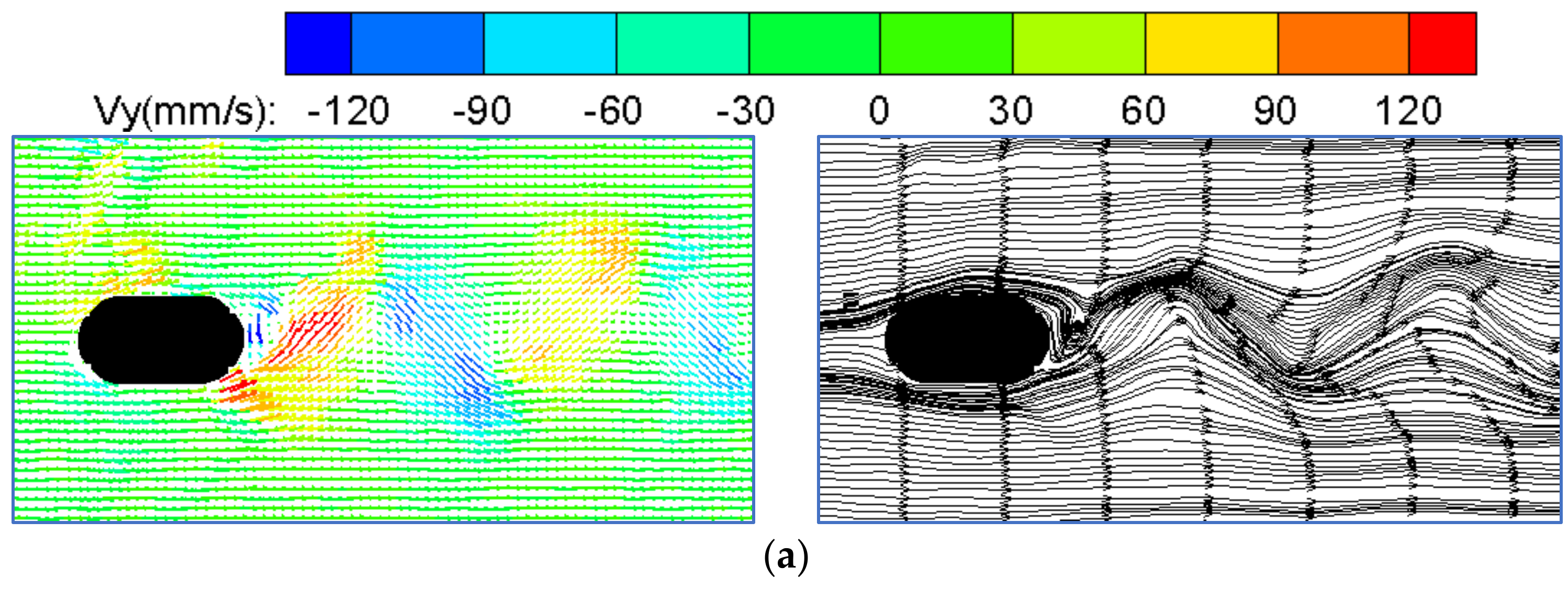
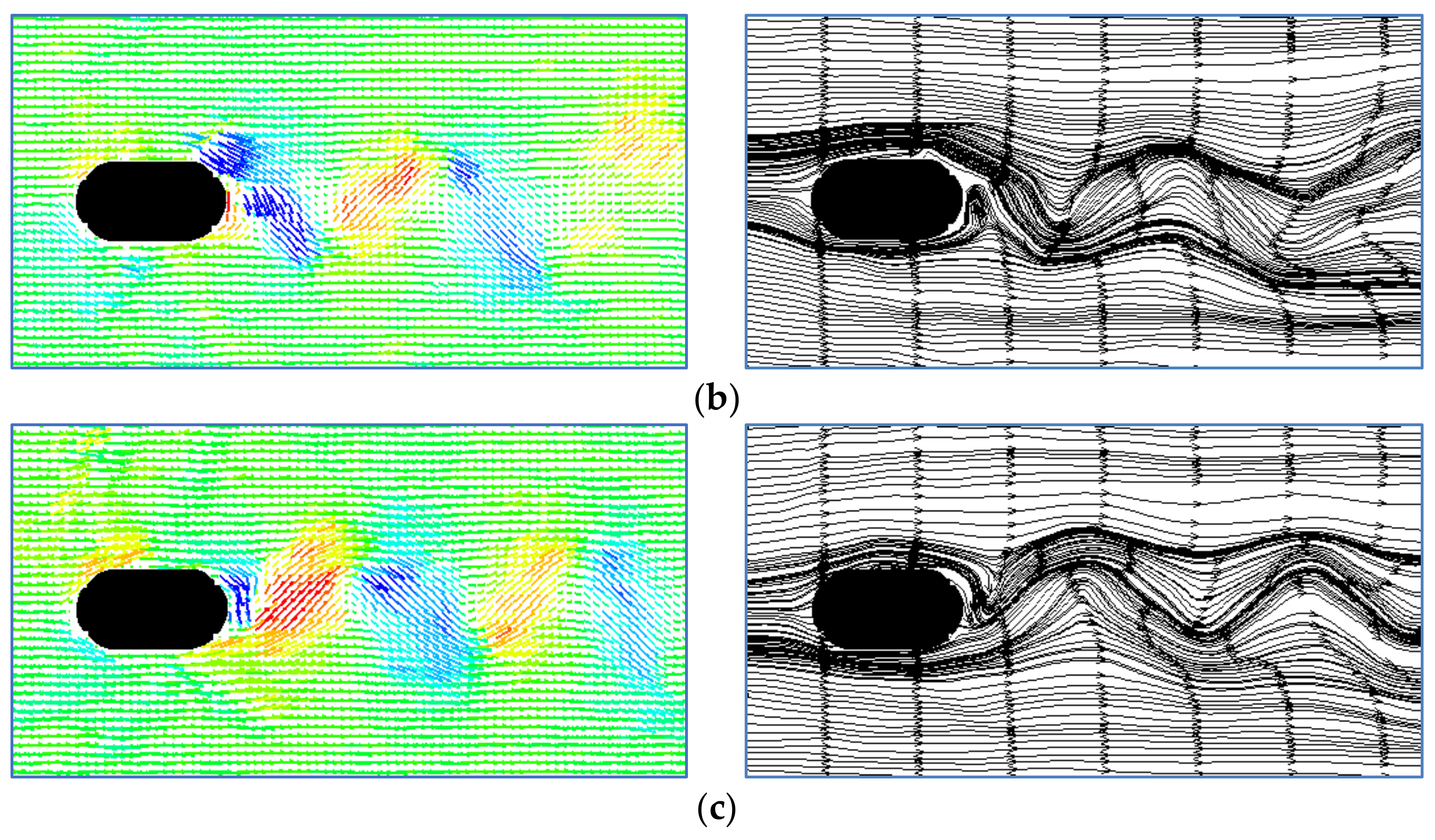
- Analysis of the flow around a pier when the flow angle of attack is 0°
Figure 4a–c show the development of the vortex systems at different moments of the flow around the round-ended pier; the transverse flow velocity Vy is in the legend, in mm/s. The changing process of the ADV measurement probe from Figure 4a–c shows that when α = 0°, the trailing vortex of the round-ended pier alternately falls off and forms a zigzag streamline. At T = 0 s, the boundary layer of the flow around the right side of the pier separates and forms a wake vortex, which then falls off downstream. When T = 0.387 s, a vortex is formed around the left side of the pier, and the flow states at these two moments have an approximate mirror image relationship based on the pier axis. When T = 0.780 s, the flow pattern is the same as that when T = 0 s; therefore, it can be concluded that the quasi-period of vortex formation and shedding around the circular end pier is approximately 0.78 s when α = 0°.
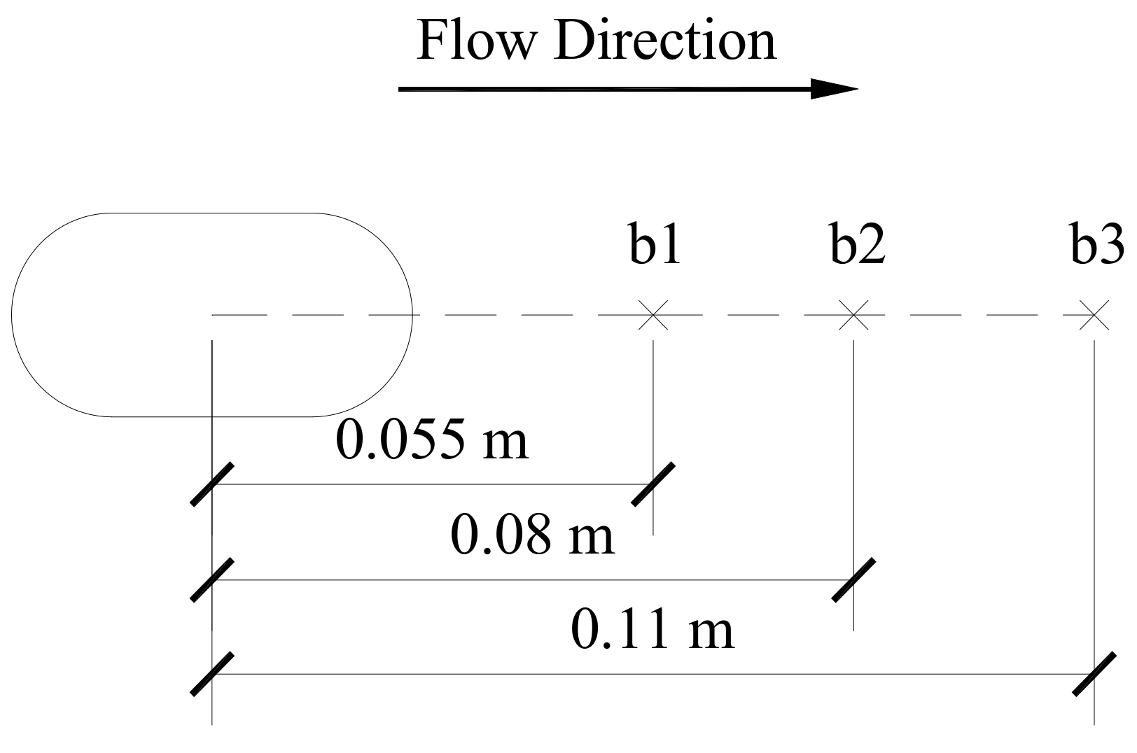
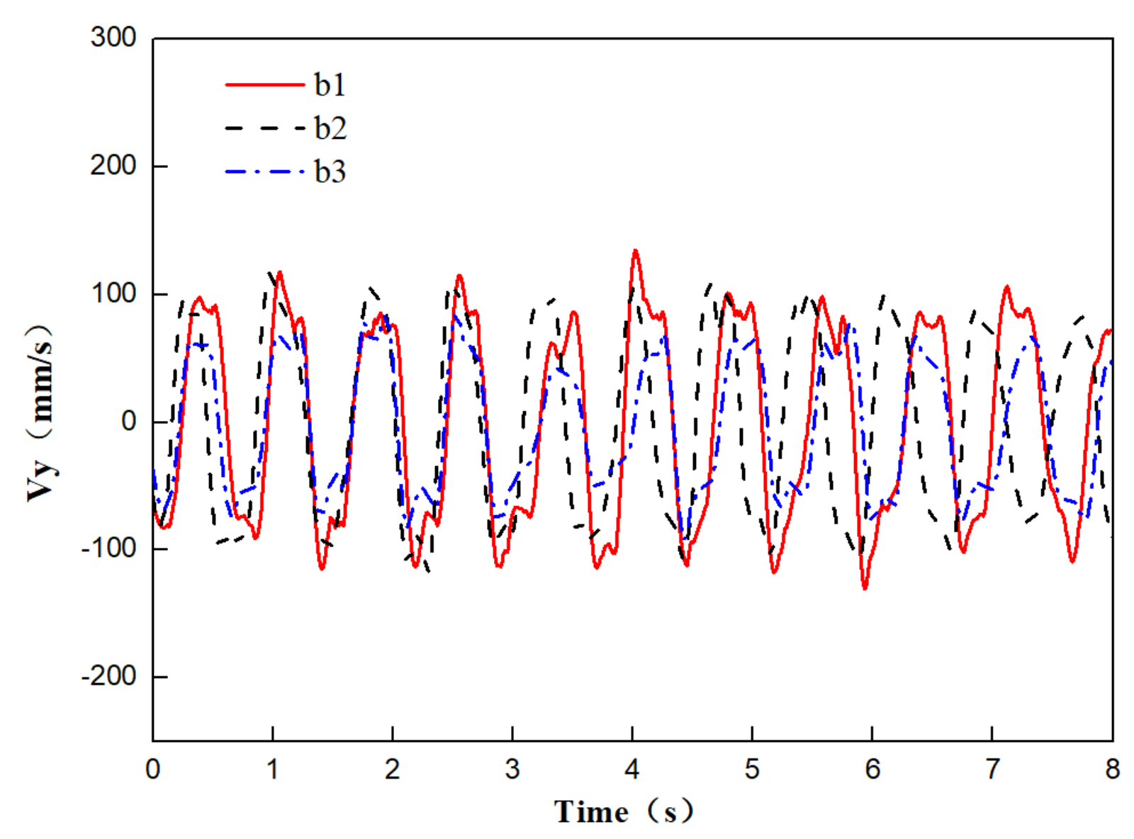
Figure 5 shows the measurement points of the ADV. Figure 6 shows the change curves of the measured transverse flow velocity over time at b1 (0.055 m), b2 (0.08 m), and b3 (0.11 m) downstream of the pier center. B1 is located at the junction of the trailing vortex and the first shedding vortex downstream of the pier, and the projection point of the midpoint of the two vortex cores on the pier axis is taken. B2 is located at the projection point of the first shedding vortex core on the pier axis. B3 is located at the projection point of the second shedding vortex core on the pier axis. Combined with the flow regime change rule shown in Figure 4, the fluctuation time of the transverse velocity duration curve behind the pier is consistent with the trailing vortex shedding time in the flow regime, which is approximately in the range 0.7–0.8 s. The transverse velocity curve behind the pier can reflect the quasi period of vortex shedding. From the peak value of the transverse flow velocity at b1–b3, it is found that the peak transverse flow velocity at b1 is the highest, approximately 0.1 m/s. The peak transverse flow velocity decreases gradually from b1 to b3, reflecting the energy dissipation process of vortex shedding.
- Effect of flow angle of attack on the flow pattern around the round-ended pier
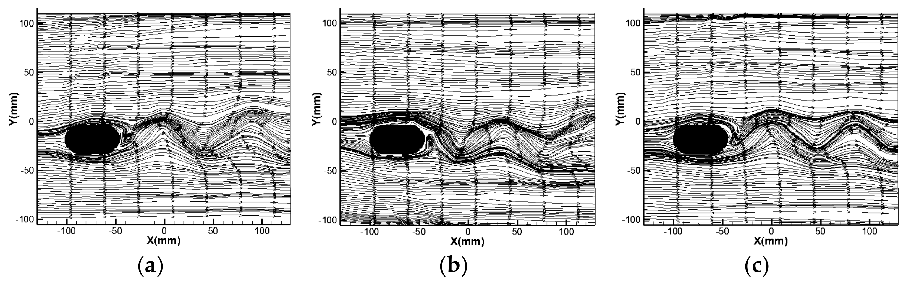
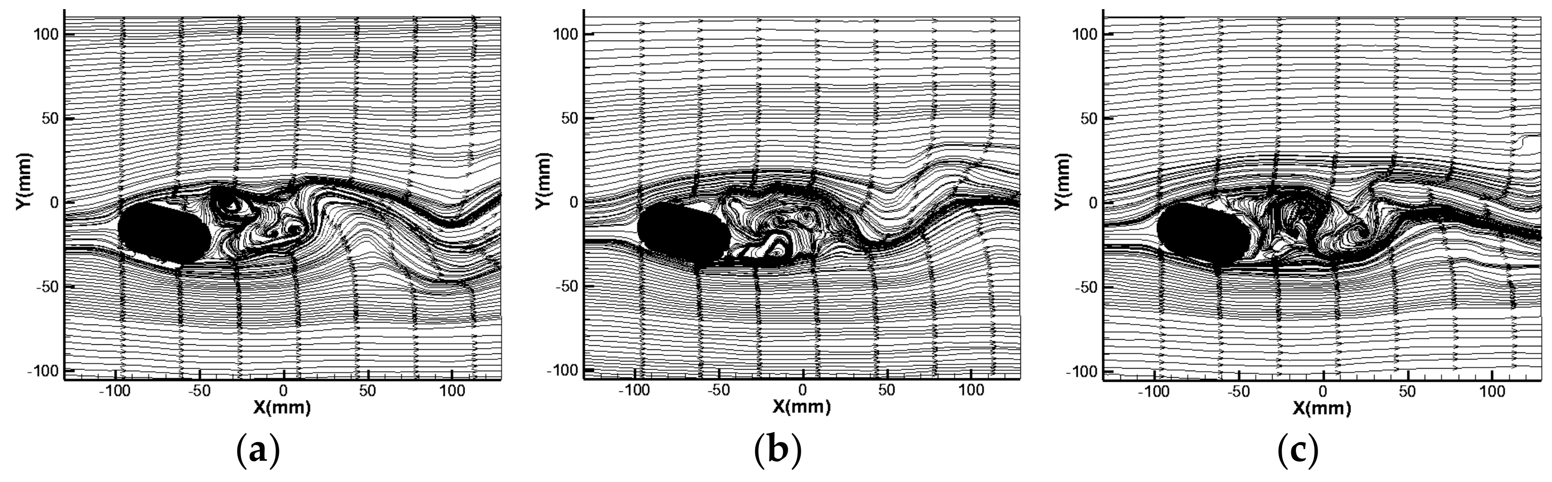
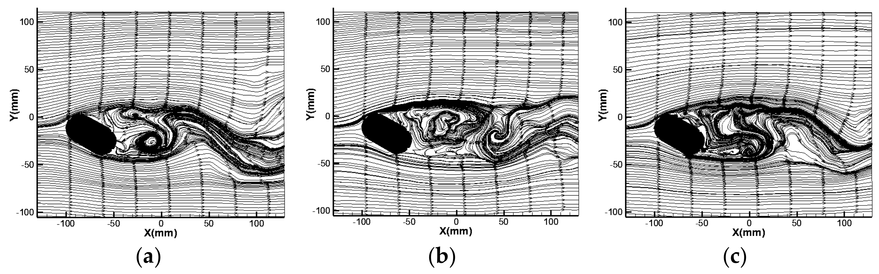
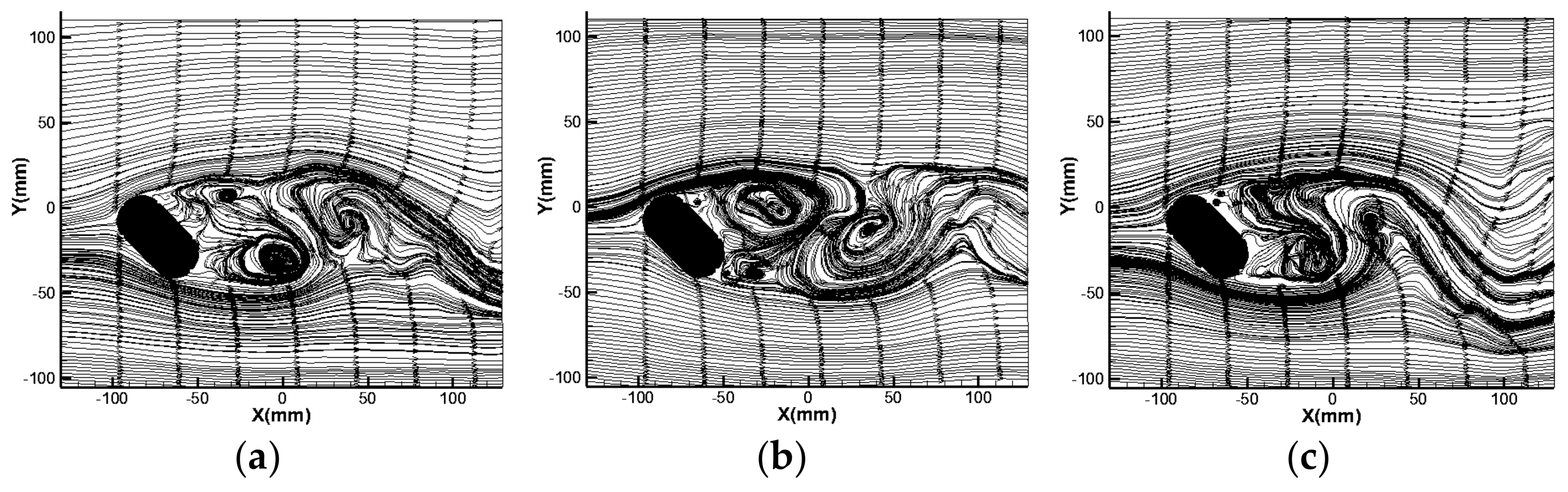
Figure 7, Figure 8, Figure 9 and Figure 10 show the instantaneous flow patterns around a round-ended bridge pier with flow angles of attack of 0°, 15°, 30°, and 45° in a quasi-period. As shown, with the increase in α, the range of the wake vortices on both sides of the pier clearly increases in both the flow and lateral directions. The separation point of the flow around the up flow side of the bridge pier is delayed, while the separation point around the back flow side is advanced. The range of the wake vortices formed on the back flow side of the bridge pier is wider than that on the up flow side, and the gap between the range of the wake vortices on both sides clearly increases with the increase in α. In addition, the trailing vortex shedding period increases significantly with the increase in α, and the trailing vortex shedding period is the slowest when α = 45°, i.e., T = 1.592 s. It is difficult to obtain the law of the pressure difference on both sides of the bridge pier with α from this test.
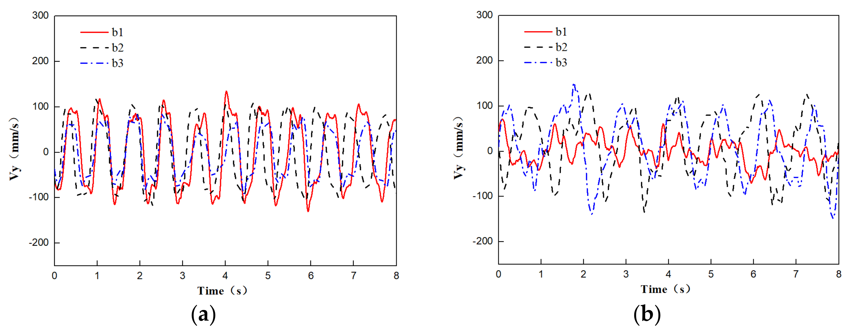
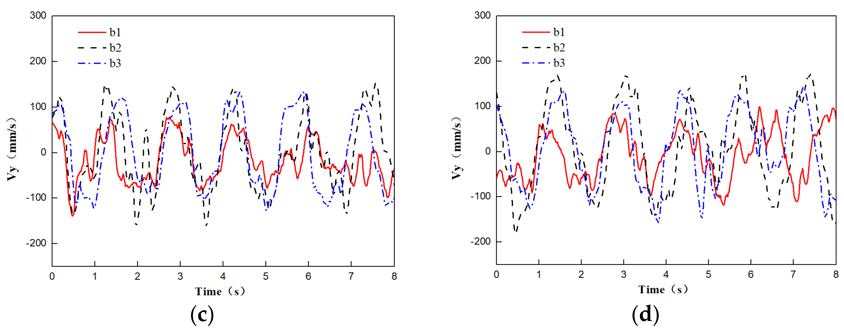
Figure 11a–d show the lateral velocity–duration curves for regions 0.055, 0.08, and 0.11 m downstream from the center of the bridge pier, measured using the ADV. As shown, with the increase in the flow angle of attack α, the pseudo-period of vortex shedding around the flow tail is consistent with the flow state judgment made using Figure 7, Figure 8, Figure 9 and Figure 10, which are approximately 0.8, 1.4, 1.5, and 1.6 s, respectively. When α = 0°, b1, b2, and b3 have clear positions, and the transverse velocity duration curve shows evident quasi-steady periodic characteristics. b1 is located at the junction of the trailing vortex and the first shedding vortex, and its transverse velocity peak is the highest. The transverse velocity peak at b2 and b3 decreases successively. With the increase in α, the range of the wake vortices on the left and right sides of the pier gradually changes; b1 and b2 are embedded into the range of the wake vortices successively; and the peak value transverse velocity at the three positions changes, from decreasing in turn, as shown in Figure 11a, to increasing in turn, as shown in Figure 11d.
2.2. Physical Model Test of Ship–Bridge Intersection
2.2.1. Test Model and Equipment
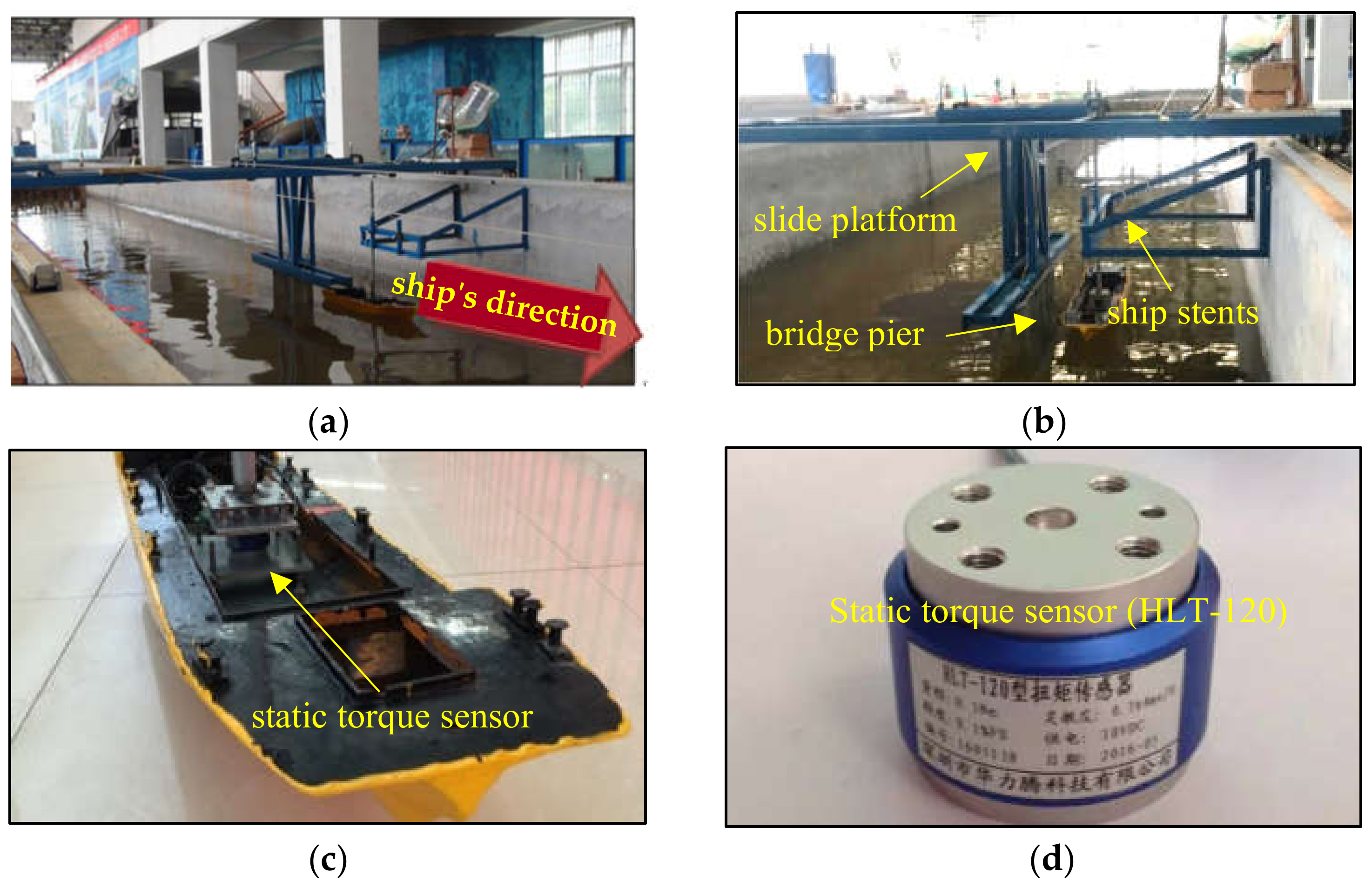
Figure 12a,b shows the ship–bridge intersection model. Figure 12c shows the ship model. Figure 12d shows the static torque sensor. The static water relative test method was adopted in the physical model test, to simulate the state of an unpowered ship passing through the bridge pier in the waterway with a river flow rate of 2 m/s, and the transverse distance between the ship and the side wall of the bridge pier was approximately one-times the diameter of the bridge pier. The test model was a 1:50 generalized flume model, and a 500T class ship model, commonly used in the Xiangjiang River, was adopted. During the test, an adjustable three-phase asynchronous motor was used to pull the wire rope fixed on the block, to drive the pier under the block and let the ship model pass through at a uniform speed. The bow roll moment of the ship model was collected using a static torque sensor.
2.2.2. Analysis of the Test Results
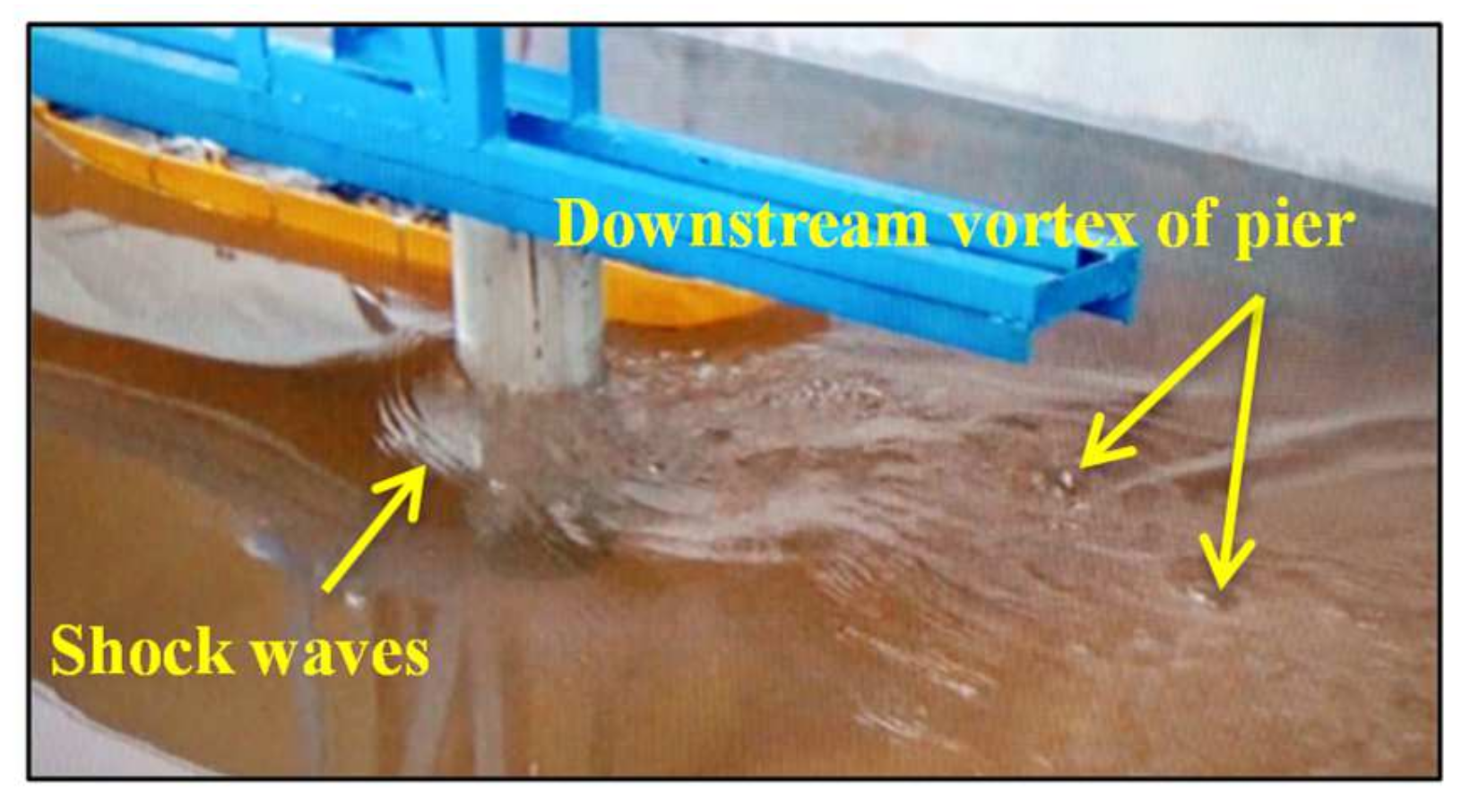
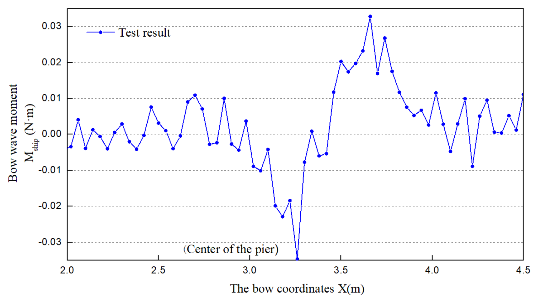
From the physical model tests, the numerical value of the forward roll moment of the ship drifting downstream was recorded. Figure 13 shows a schematic of the wake around the pier. Figure 14 shows the schematic of the ship’s bow roll moment along the path. As shown, under the influence of the complex flow regime around a ship pier, the numerical change in the bow roll moment follows a certain rule: while the bow approaches the pier, the bow roll moment of the ship increases gradually, and when the bow is near the pier, the bow roll moment reaches a positive peak, and the ship turns counterclockwise. When the bow passes through the pier, the bow begins to be affected by the pier tail vortex (Figure 13), and the ship rotates clockwise. The bow roll moment starts to decrease and reaches a negative peak before the ship completely passes the pier. When the stern reaches the position of the pier, the stern enters the wake vortex region, and the bow roll moment again reaches the positive peak value. The second positive peak value is higher than the first positive peak value and negative peak value; therefore, the ship has the highest force influence at this position. After the ship passes the pier completely, the bow roll moment fluctuates near the initial value of 0, due to the effect of street shedding of the trailing vortex of the pier.
3. Numerical Modeling
Physical model test conditions are limited, as they require a high labor cost and a considerable amount of time. It is difficult to conduct multiple groups of tests simultaneously, and the test results only reflect a part of the objective law; the form of the expression is single. In comparison, after a numerical simulation is effectively validated, it can efficiently simulate multiple working conditions simultaneously and obtain richer calculation results and analysis data. In this study, Fluent software was used to simulate the hydrodynamic problems of bridge piers with different flow angles of attack; this section presents the relevant details.
3.1. Establishment of a Geometric Model and the Arrangement of Simulation Groups
The motion of a ship is associated with six degrees of freedom: translation motions in the X, Y, and Z directions, and rotation about the three directions based on these coordinate axes. This study is concerned with the transverse drift (translation in the Y direction) and rotation (rotation about the Z axis) under the influences of transverse flow and vortex negative pressure structure to ensure navigable safety in areas where ships and bridges intersect. Thus, the model was generalized on the basis of the properties of the transverse drift and rotation. Only three degrees of freedom (translation motion in the X and Y directions and rotation about the Z axis) are allowed, and the model is simplified into a 2D plane.
3.1.1. Analysis of Test Results
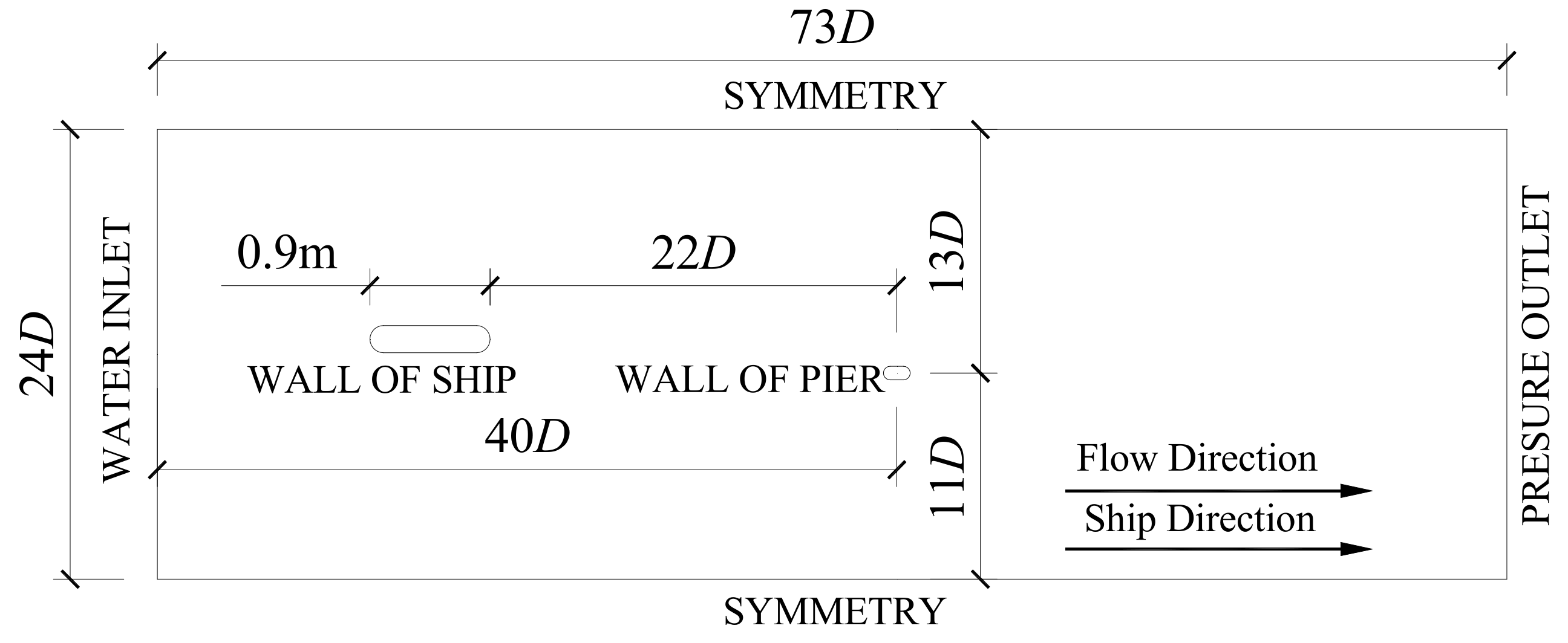
The Design Modeler software in Workbench was used to construct a 2D geometric model of the ship–bridge intersection, with a geometric scale of 1:50. Figure 15 shows a schematic of the geometric model, in which the long axis of the round-ended pier d = 0.2 m, the pier width b = p = 0.1 m, and the hydraulic diameter of the pier section D = 0.138 m for the characteristic length. For the ship size, we used the common 500 T barge for water transport in Xiangjiang River, and the model size was 0.9 m × 0.2 m (length × width). The position that remains unaffected by the development of the vortex street around the pier was selected as the boundary of the computational domain. The distances between the two sides of the boundary and the pier center were 13D and 11D, respectively, and the distance between the downstream boundary and the pier center was 33D. Considering the interaction between the ship and the water flow in the initial flow field, and to avoid the disturbance of the water flow affecting the waters around the pier, the distance between the upstream boundary and the pier center was set to 40D, and the distance between the ship and the upstream gauge boundary was set to 11D.
3.1.2. Numerical Simulation
In this numerical simulation, the river velocity V was set to 0.283 m/s, the opposite shore speed of the downstream ship was set to 0.566 m/s, and the pier width b was set to 0.1 m. Under different transverse spacings between the ship and bridge, the ship movement on the left and right sides of piers, with different flow angles of attack of the water flow, was simulated. There were 21 groups of simulations and one verification simulation with an unpowered ship (Table 2).
3.2. Governing Equation
3.2.1. Flow Governing Equation
The RNG k-ε turbulence model has a good accuracy in simulating the hydrodynamics of ships. The number of encrypted grids required on the wall is small, and the calculation efficiency is high. In this study, this turbulence model was used for the numerical simulation of the ship–bridge hydrodynamic problems. The RNG k-ε governing equation is as follows:
Continuity equation:
RANS equation:
k equation:
ε equation:
In Equations (1)–(4), k is the turbulent kinetic energy, ε is the dissipation rate, is the fluid density, is the velocity, is the pressure, t is the time, is the dynamic viscosity of the fluid, is the Reynold’s stress, is a diffusion coefficient, and are constants () is the turbulent kinetic energy generation term, and is a model constant (). , including the constants , , , , is the time average strain rate, and is the eddy viscosity coefficient, in which 0.0845.
The finite volume method (FVM) was used to discretize the above governing equations in the computational domain, and the SIMPLE algorithm was adopted. The discretization scheme used was the second-order upwind scheme.
3.2.2. Flow Governing Equation
In this study, the movement of the ship passing the pier was considered a rigid body movement, and this process was calculated using the torque and center of gravity displacement formula in the rigid body six-DOF control equation, which is as follows:
In Equations (5)–(7), is the translational motion of the center of gravity per unit time, m is the mass, and is the force vector due to gravity, is the angular velocity vector in the object coordinate system, L is the rigid body inertia tensor, is the moment vector in the object coordinate system, is the moment vector in the inertial coordinate system, and R is the coordinate transformation matrix, expressed in Equation (8):
is equal to in our transformation matrix, and is equal to , and , , and are the Euler angles about the Z, Y, and X axes, respectively.
3.3. Meshing Methods and Application of Self-Compiled UDFs
3.3.1. Grid Division and Dynamic Grid Method
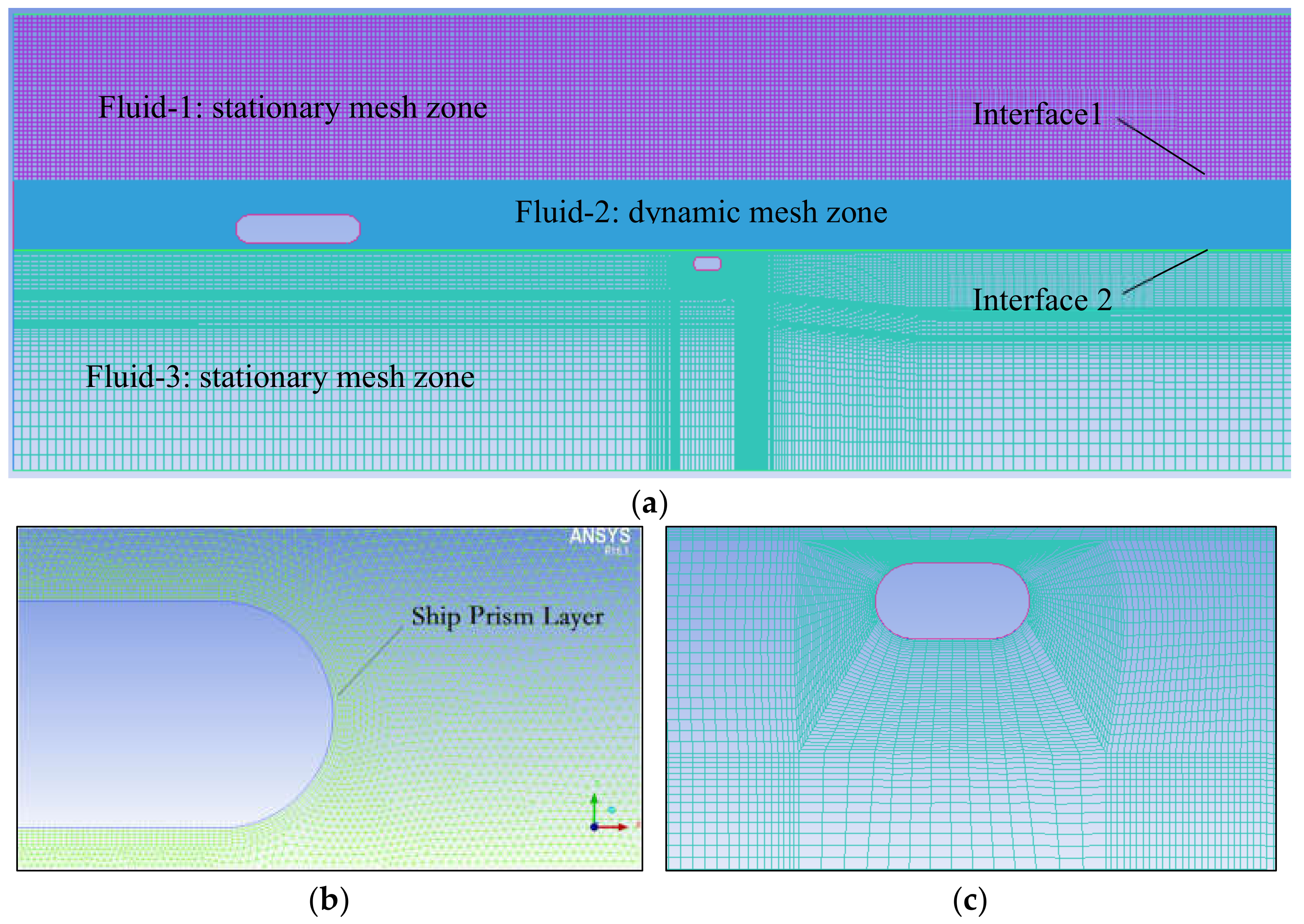
Ship motion involves the motion of the fixed wall boundary, and it should typically be calculated using the dynamic grid method. In this study, the distance of ship movement far exceeds the size of the grid, each part of the ship is affected differently by the force of the water flow, and the motion law is complex. Therefore, the spring smoothing and local reconstruction method built in Fluent was used for a dynamic simulation of the grids. The local reconstruction method requires the regional mesh to be triangular (2D) or tetrahedral (3D), and the computational domain can be divided into moving and stationary mesh zones, on the premise of ensuring accuracy. In Figure 16a, Fluid-1 and Fluid-3 are the stationary mesh zones, which are divided into quadrilateral structural grids using the O-block partition method, and Fluid-2 is the dynamic mesh zone, which is divided into triangular nonstructural grids. To accurately capture the complex flow field near the ship and pier, the boundary grid of the ship and pier was encrypted. The height of the first-layer grid node was calculated as Δy = 0.0017734 m, using the standard wall function method. Figure 16b,c show diagrams of the near-wall grid of the ship and pier.
3.3.2. Self-Compiling UDF Process
In this study, the user defined function (UDF) in Fluent was used to write commands in C language, to simulate the displacement and force during ship movement. In the Fluent software of DEFINE_CG_MOTION (name, dt, vel, omega, time, dtime), the macro moment of inertia of the rigid body, quality, and other related parameters are defined, the degrees of freedom of the ship are only in the three directions of yaw, pitch, and roll. In the simulation process, each time step calls the ship’s linear velocity, angular velocity, and Euler angle in the previous time step through the macro; these are then substituted into the rigid body control equation to obtain the new center of gravity position and moment of the ship. The two parameters are here converted to the inertial coordinate system to calculate the linear velocity, angular velocity, and center of gravity position in the next time step; they are then converted to the onboard coordinate system parameters for storage. The position of the ship’s center of gravity and the rocking moment of each time step are derived from Compute_Force_And_Moment (domain, t, x_cg, f_body, m_body, TRUE) macro, in which x_cg represents the coordinates of the ship’s center of gravity, f_body is the yawing force acting on the ship, and m_body is the rocking moment of the ship.
4. Verification and Analysis of Numerical Simulation Results
4.1. Verification of Numerical Simulation Results
4.1.1. Verification of Flow Field and Vorticity Field around Flow
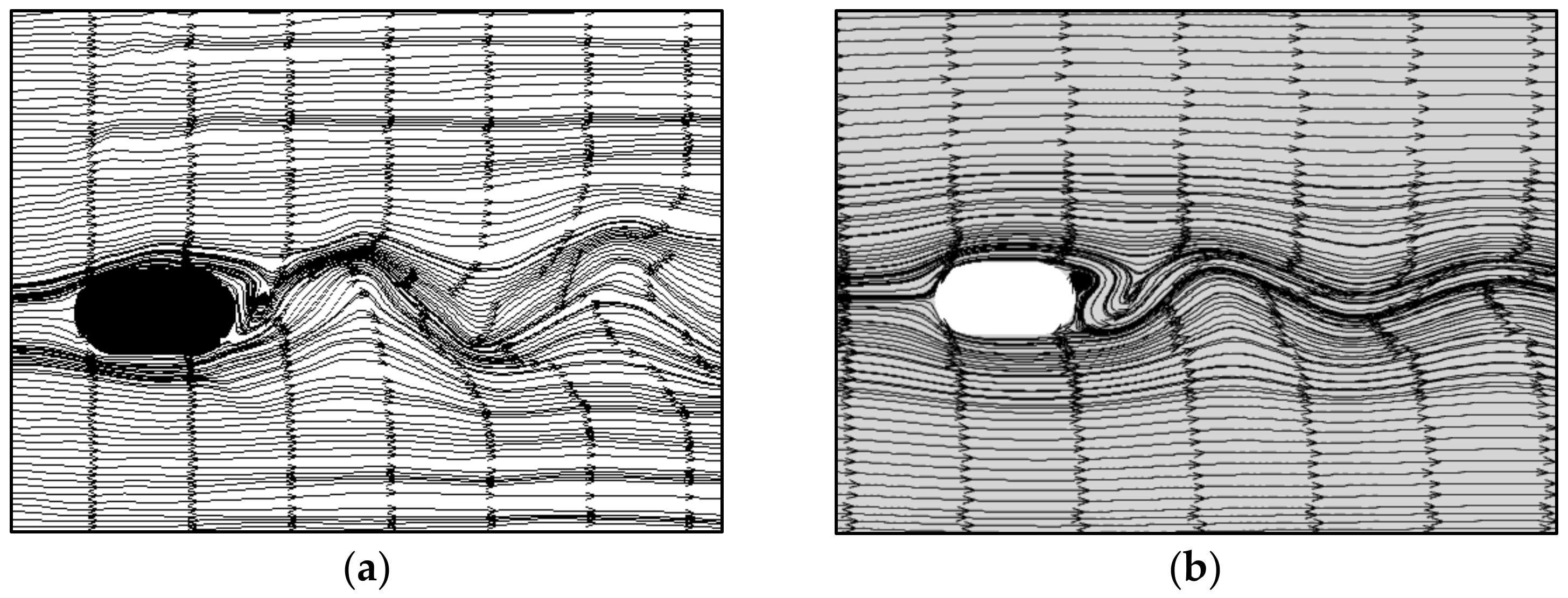
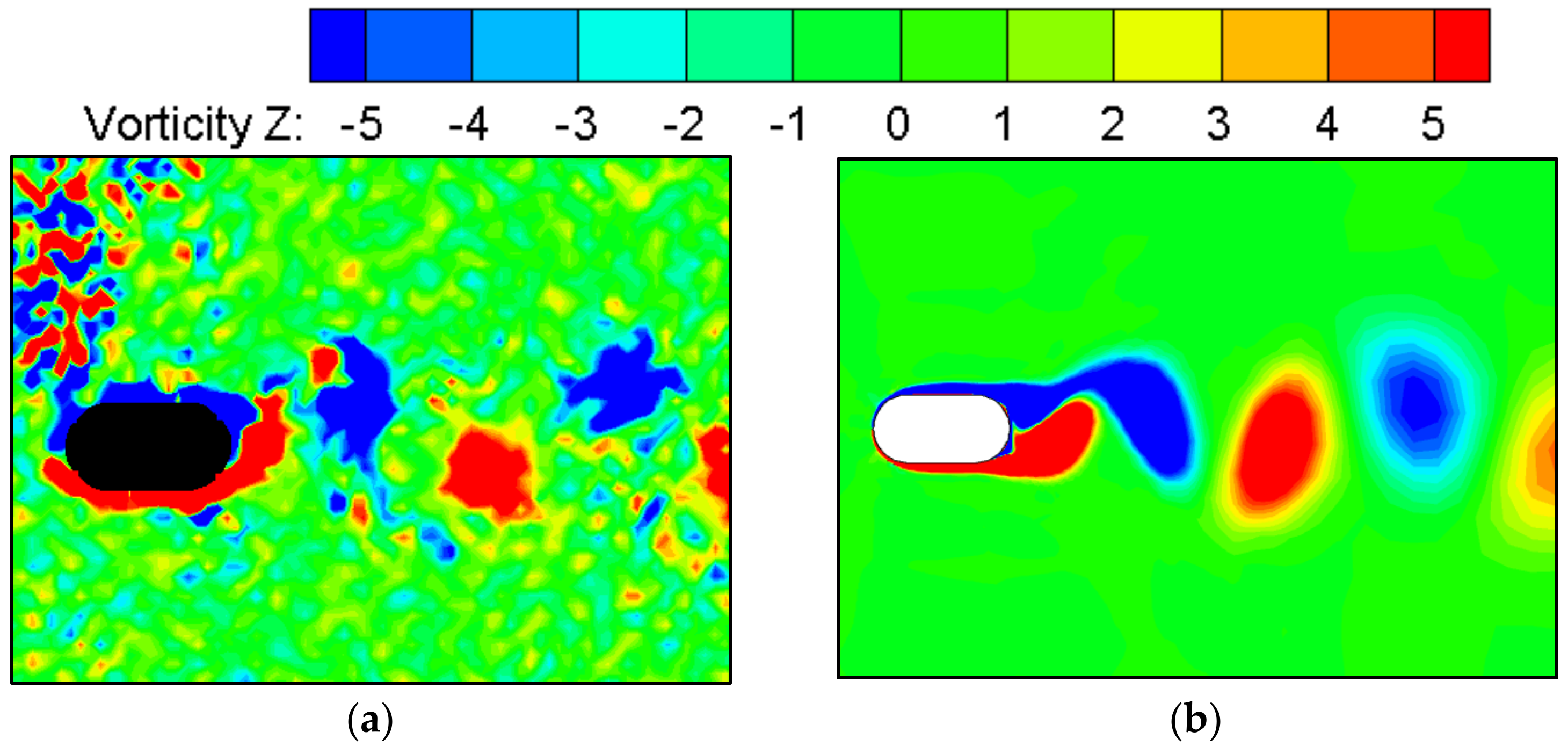
Figure 17 and Figure 18 show the flow pattern and vorticity of the flow field around the pier, obtained by numerical simulation and PIV-based physical model test, respectively. As shown, when the flow rate of the model river is 0.141 m/s, the trailing vortex range, vortex shedding position, and tortuous streamline obtained by the numerical simulation are consistent with the flow pattern results of the test. The vorticity distribution of the wake vortex is consistent with the post-processing results of the test.
4.1.2. Verification of Trailing Vortex Shedding Frequency and Transverse Velocity behind a Round-Ended Pier
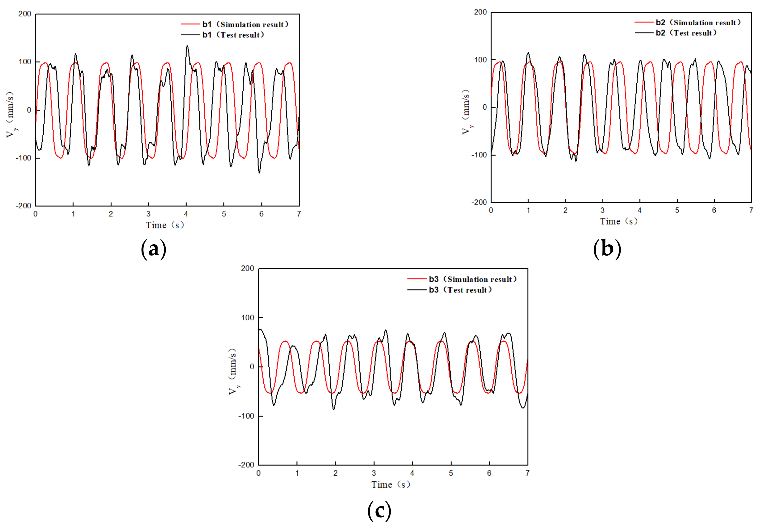
The transverse velocity at b1 (0.055 m), b2 (0.08 m), and b3 (0.11 m) on the back surface of the round-ended pier (α = 0°) without a ship was simulated. Figure 19 shows a comparison between the simulation results and ADV test measurement results. When the river flow rate is 0.141 m/s, the fluctuation frequencies of the transverse velocity curves of the two are close, and the peak value is similar. As the measuring point shifts to downstream of the bridge pier, the peak value of the transverse velocity decreases, reflecting the velocity change rule in the dissipation process of trailing vortex shedding.
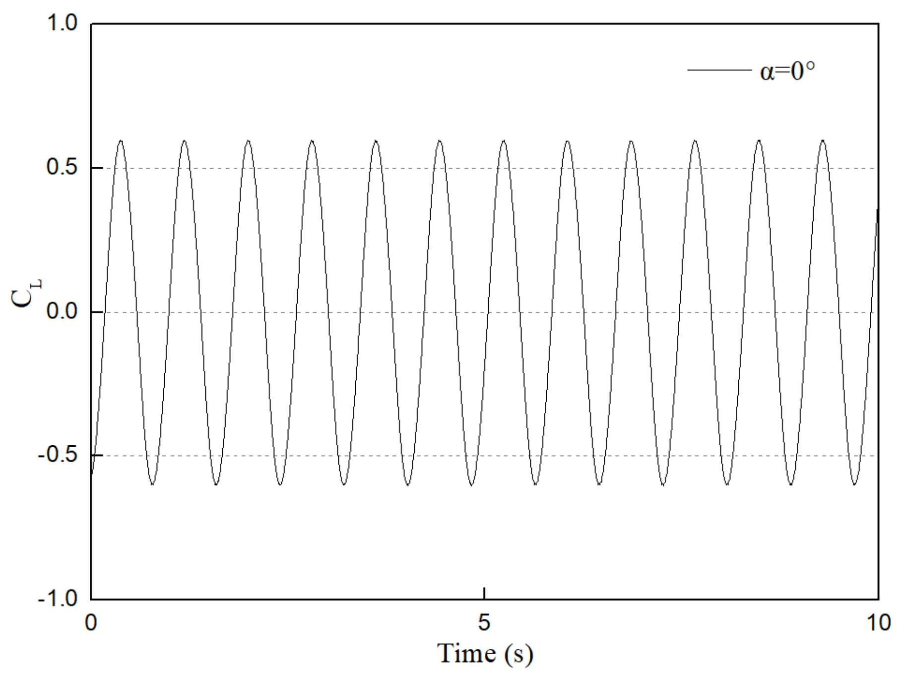
The periodic successive separation of the boundary layer around the pier leads to a dynamic pressure difference on both sides of the pier. FL, which is the force perpendicular to the flow direction of the pier, fluctuates, and its fluctuation frequency is consistent with the wake vortex shedding frequency and transverse flow velocity fluctuation frequency. In this study, the fluctuation period of the lift coefficient around the flow was found to be 0.8 s through simulation (Figure 20), which is consistent with the experimental result of 0.78 s discussed in Section 3.1.2. Here, V is the river velocity, and D is the characteristic length of the blunt body.
In conclusion, the flow pattern, vorticity field, and wake vortex shedding period predicted by the numerical simulation in this study are in good agreement with the physical model test results, indicating that the established model and numerical method can ensure the accuracy of the simulation of the flow around the pier.
4.1.3. Numerical Verification of Bow Roll Moment and Its Evolution Law
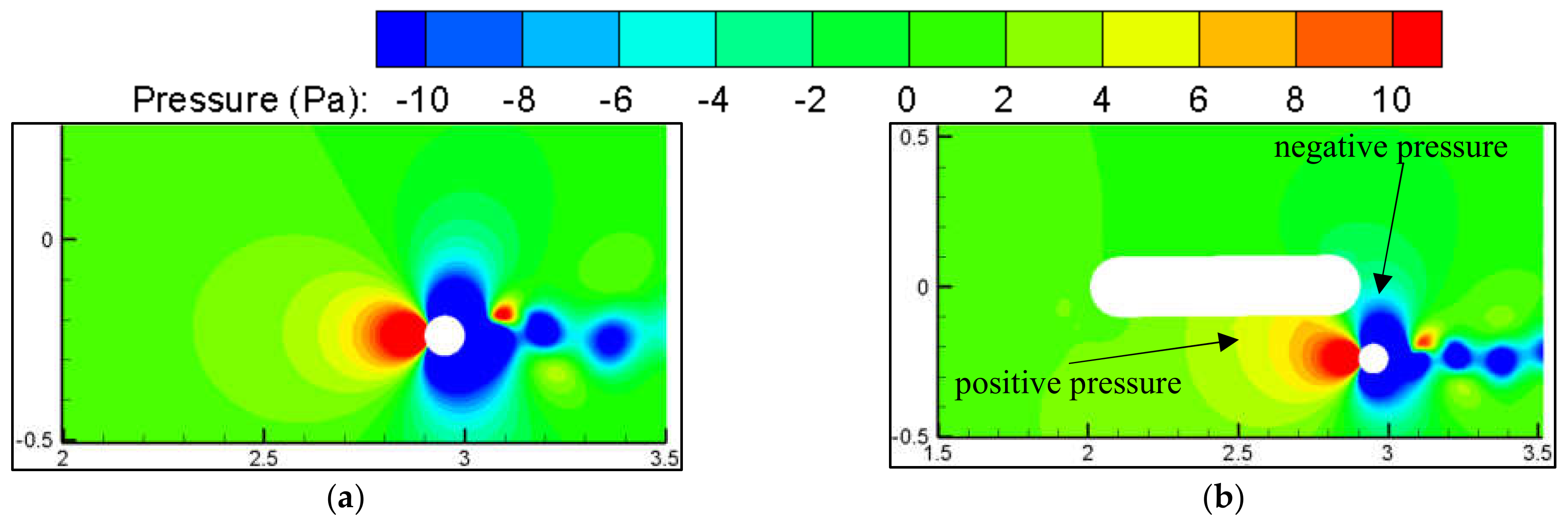
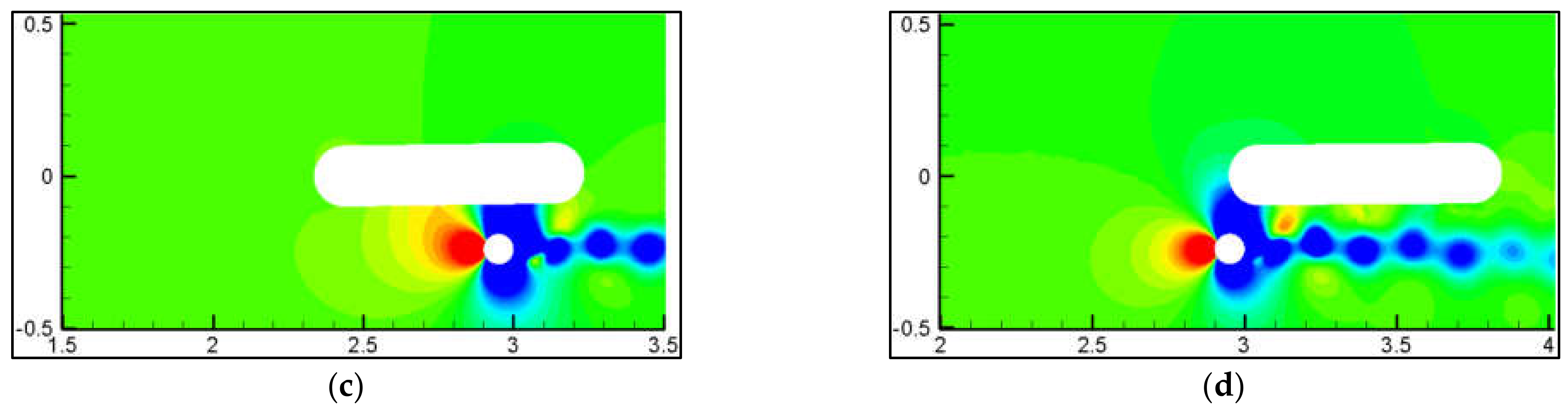
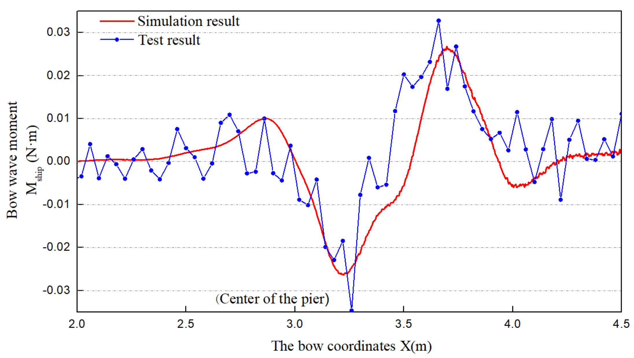
Based on the model test conditions of ship–bridge crossing in the verification group, the drifting process of the ship passing through the bridge pier was simulated when the inlet flow rate was 0.283 m/s, and the transverse distance between the ship and the bridge pier was one-times the diameter. Figure 21 shows the water pressure distribution around the pier. Negative water pressure attracts the ship, while the positive water pressure repels it. Figure 22 shows a comparison between the numerical simulation results and physical model test results of the ship’s roll moment. As shown, the positive and negative water pressures acting on the ship can reflect the change law of the roll moment as the ship passes the bridge pier. The numerical simulation results show that the curve and peak values of the bow roll moment are similar at different ship positions.
In summary, the flow field around the flow predicted by the numerical simulation in this study is in accordance with the actual situation, and the calculation results of the force and moment on the ship are also accurate. Hence, the model and numerical method can be used to simulate the process of ship–bridge crossing in the other groups.
4.2. Verification of Numerical Simulation Results
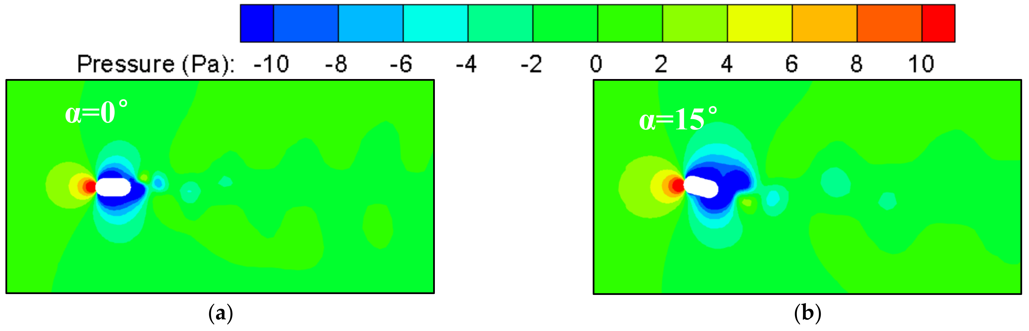
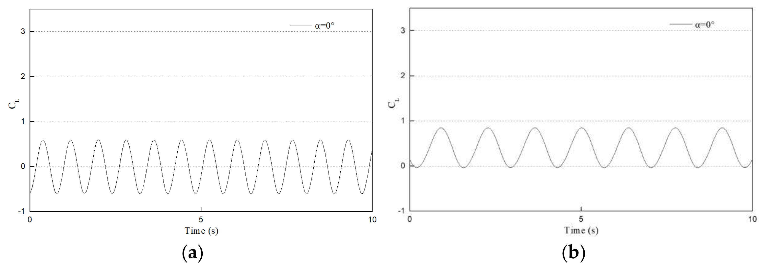
The water pressure around the pier is a direct factor for judging ship motion and force variations. The water pressure distribution around the round-ended pier with different flow angles of attack can be obtained by numerical simulation. Figure 23 and Figure 24 show the water pressure distributions around the round-ended pier with α = 0° and α = 15°, respectively, and the diurnal variation in the lift coefficient of the flow around the pier. The results show that, when the flow angle of attack is less than 15°, the range of the positive water pressure area does not change significantly and is located upstream of the pier, and the range of the negative water pressure area behind the pier increases with the increase in the trailing vortex range on the back side of the pier. Whether the stress on both sides of the pier is uniform can be judged by the amplitude of the positive and negative CL fluctuations. As shown in Figure 24, when the flow angle of attack increases from 0° to 15°, the lift fluctuation period of the bridge pier increases, and the lift direction almost points toward the back flow side. This is because the separation point of the boundary layer on the back flow side advances, while the separation point on the upstream side of the pier drops back, because of which, the upstream side of the pier is subjected to a relatively stable water pressure and counteracts the periodic negative water pressure, due to the wake vortex on the back flow side.
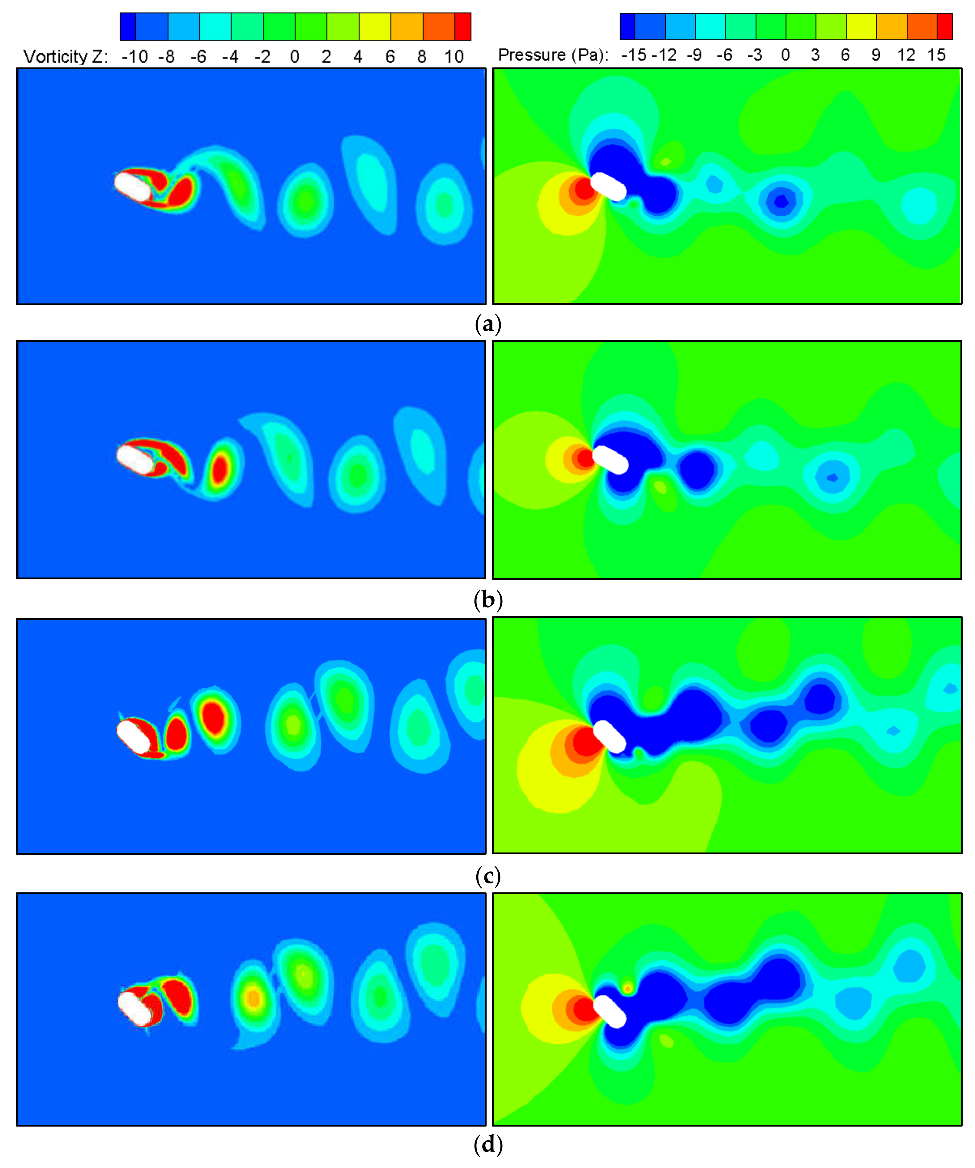
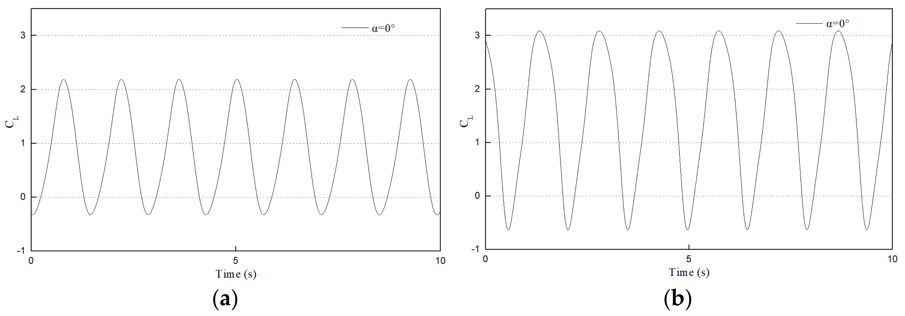
Figure 25 and Figure 26 show the vorticity field, water pressure field, and diurnal variation of the flow CL around the pier within half a period, when the flow angles of attack of the round-ended pier are α = 30° and α = 45°. As shown in Figure 25, when the flow angle of attack is above 30°, the position of the positive water pressure area in front of the pier begins to swing left and right, under the influence of the formation and shedding of the trailing vorticity on the back flow side. The oscillation period is the same as the shedding period of the trailing vortex of the pier, and the oscillation amplitude upstream side of the pier is high. It can be concluded that the positive water pressure on the upstream side of the pier is greater than that on the back side and that the area of positive and negative water pressures increases with the increase in the flow angle of attack. When α = 45°, it is evident that the shedding direction of the downstream vortex shifts to the back flow side, so that the negative water pressure area also shifts to the back flow side of the pier. As shown in Figure 26, the peak lift force of the pier facing the back flow side of the pier increases significantly with the increase in the flow angle of attack, and the maximum lift coefficient reaches 3.03 when α = 45°. However, the increase in the lift force toward the upstream side of the pier is small, indicating that the water pressure therein can still offset most of the periodic negative water pressure on the backflow side after the increase in the flow angle of attack.
4.3. Influence of Flow around a Round-Ended Pier with α = 0° on Moving Ship
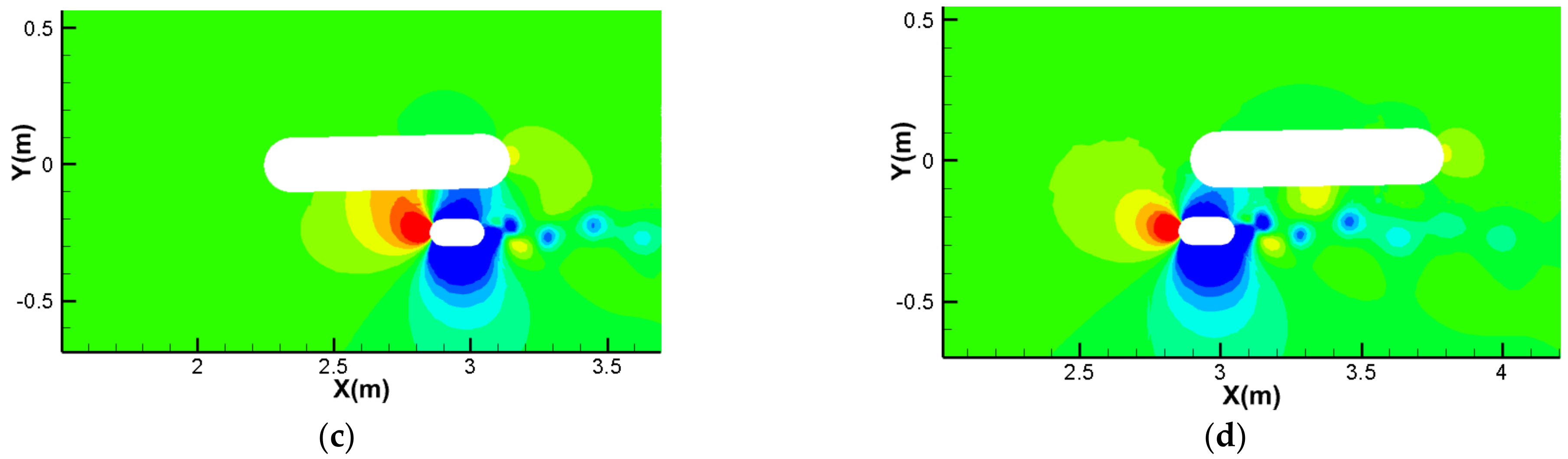
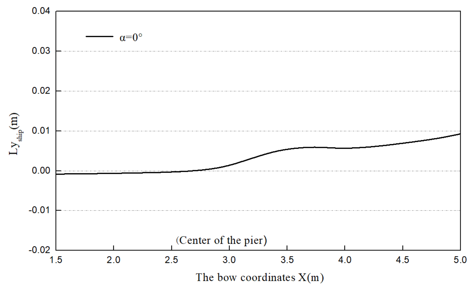
Figure 27a shows the variation rule of the bow roll moment when the ship passes the pier at an opposite speed of 0.566 m/s, under conditions where the transverse spacing between the boat and pier is 1b, the river flow velocity is 0.283 m/s, and the impact flow angle of attack is 0°. Figure 27b–d show a water pressure distribution diagram of the ship in the process of movement. Figure 28 shows the displacement curve of the ship’s center of gravity in the X and Y directions in the movement process (the positive Y direction is laterally away from the bridge pier).
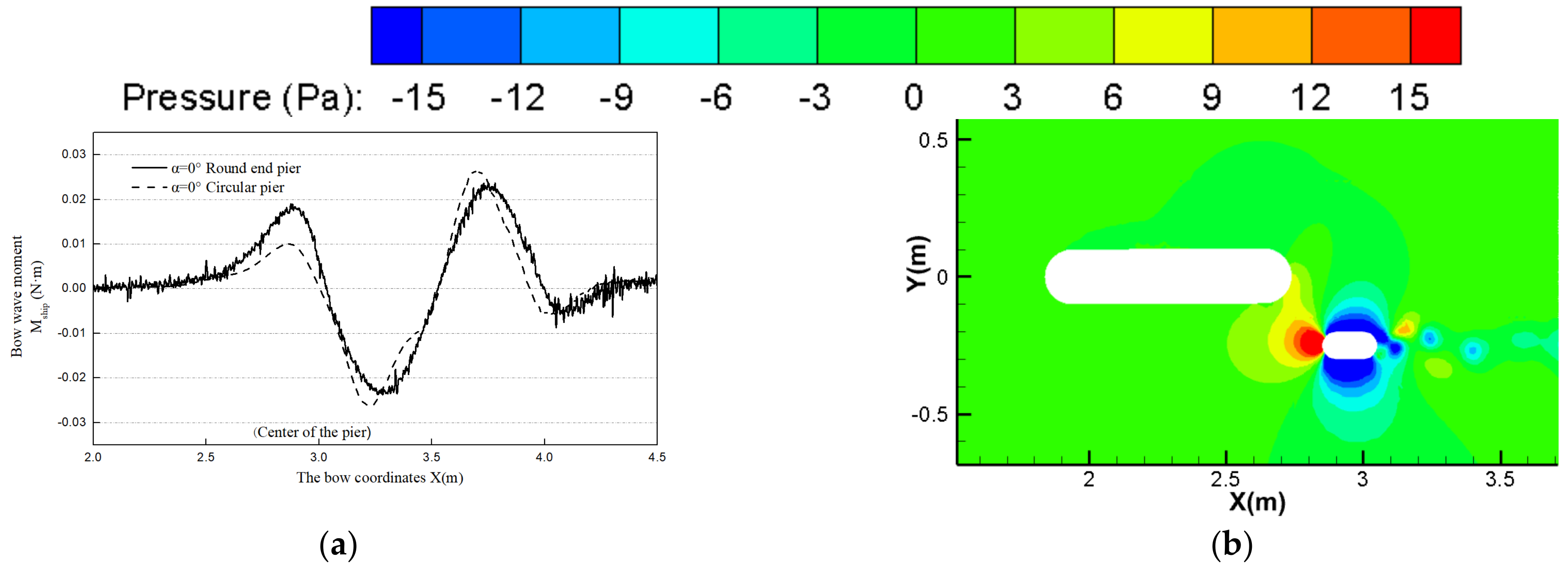
These figures show that the bow roll moment curve of the ship passing through the waters around the round-ended pier (α = 0°) is close to that of the ship passing by the circular pier. The first positive peak value is slightly greater, and the negative peak value and the second positive peak value are slightly lower. When the round-ended pier has an flow angle of attack α = 0°, the bow is subjected to positive water pressure in front of the pier when it comes to the pier head, and the bow tends to deflect away from the pier. At this moment, the bow roll moment reaches the first positive peak in the forward direction, and the ship’s center of gravity begins to shift in the Y-axis direction. When the bow comes to the side and tail of the pier, the hull begins to be affected by the forward water pressure. The bow is subjected to the negative water pressure of the wake vortex behind the separation point on the pier side. At this moment, the hull has a relatively significant clockwise rotation trend, the bow roll moment turns from positive to negative and reaches a negative peak, and the velocity of the ship’s center of gravity moving forward to the Y-axis decreases. For this process, a bulge in the displacement curve can be seen in Figure 28. When the stern passes over the pier, the stern is subjected to the negative water pressure of the trailing vortex behind the separation point on the pier side. Although the bow is also affected by the negative pressure of the trailing vortex, the negative pressure decreases with vortex dissipation after the trailing vortex falls off, so that the negative pressure on the bow is less than that on the stern. The ship will rotate counterclockwise for the second time, so that the bow roll moment reaches the second positive peak value, which is greater than the first positive peak value. After the stern moves away from the negative pressure area of the wake vortex, the ship’s axis keeps an angle with the main stream to the downstream, and the center of gravity is laterally away from the pier. Overall, the bow roll moment curve of the ship passing under the condition α = 0° is close to that of the ship passing around the pier, and the first positive peak value is slightly greater, while the negative peak value and second positive peak value are slightly lower.
4.4. Analysis of the Influence of Flow around a Circular-Ended Pier on Moving Ship
After clarifying the basic laws of the change in the bow roll moment and the position of the center of gravity as a ship passes through a bridge area, the influence of increasing the flow angle of attack of the pier on the moving ship was further analyzed. As previously stated, when α = 30°, the positive water pressure distribution area in front of the pier begins to show an evident periodic swing, which is typical. Therefore, under the condition where the river velocity was 0.283 m/s, the transverse distance between the ship and the pier was 1b, and the flow angle attack of the round-ended pier was 30°, the process of the ship passing through both sides of the pier at an opposite speed of 0.566 m/s was analyzed.
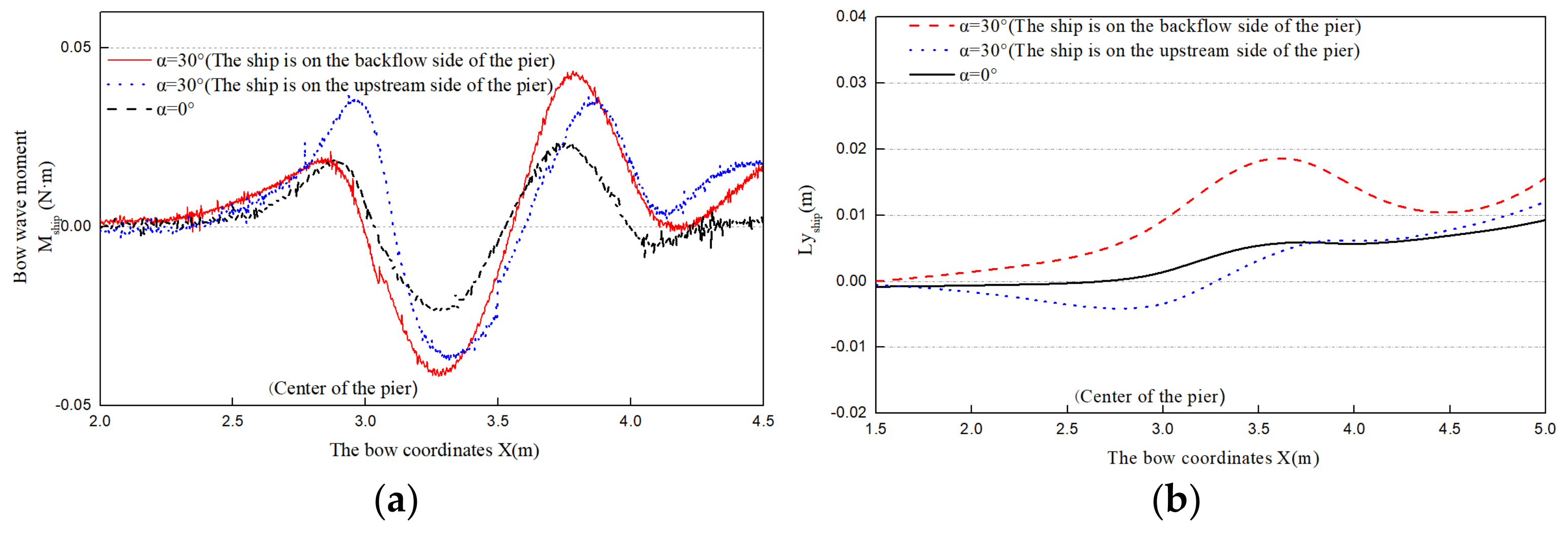
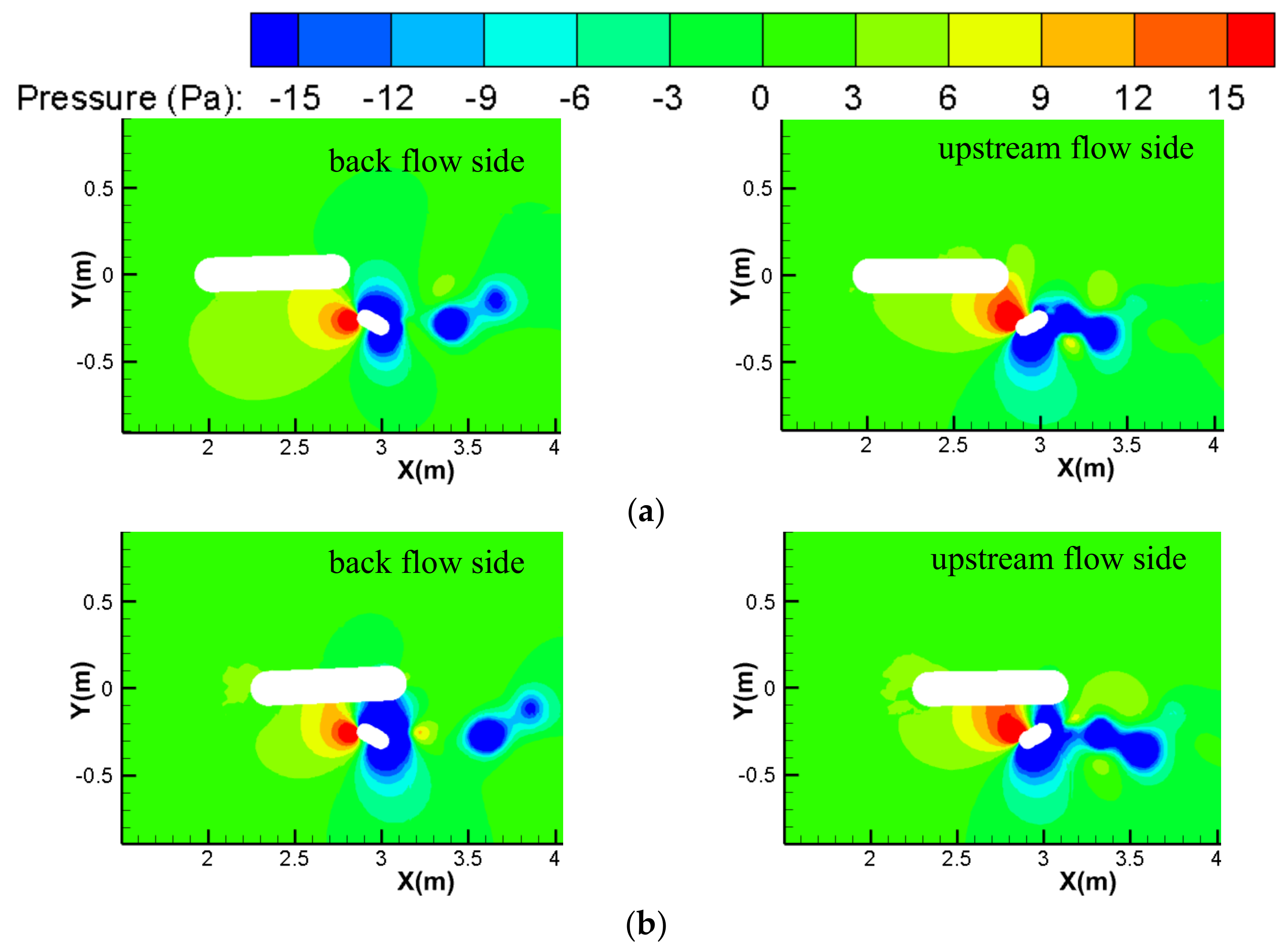
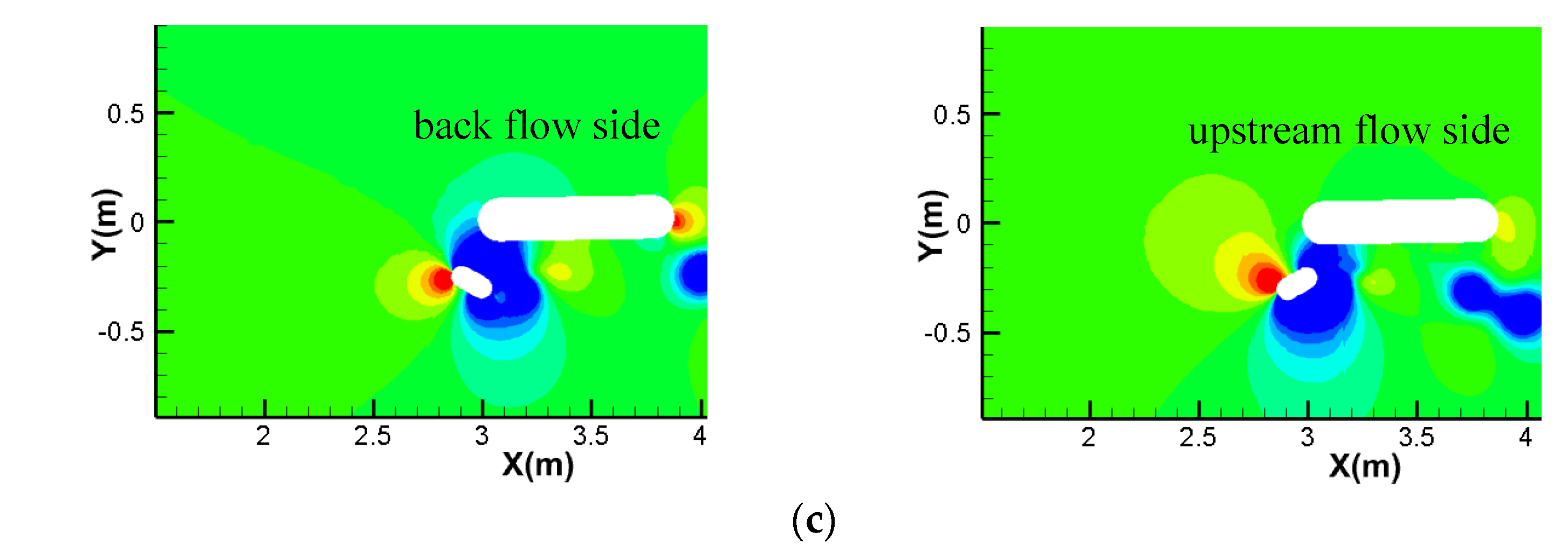
The forward pressure area in front of the pier was made to swing just to the side of the ship when the ship sails toward the pier head, to determine the initial position of the ship release in the numerical model. Figure 29 shows the curves of the bow roll moment and center of gravity position throughout the course when the ship passes by both sides of the upstream and backflow sides of the round-ended pier α = 30°. Figure 30 shows the distribution of the water pressure between the bridge and ship.
These figures show that the first peak value of the ship’s bow roll moment when the ship passes through the upstream side is much higher than that of the ship on the back side, and when α = 0° and the position of the ship’s center of gravity shifts to the negative direction of the Y-axis in advance. This is because, when the bow of the upstream side of the pier is approximately the length of the ship, the velocity in the X direction of the upstream side of the pier is higher close to the pier, due to the diversion action of the upstream side of the pier. At this time, the ship has not reached the positive water pressure area, and there is a pressure difference, due to the velocity difference on both sides of the bow, which pushes the bow toward the right bank. When the ship passes through the back flow side of the pier, the first peak value of the bow roll moment is low, which is close to that when α = 0°, and the ship’s center of gravity shifts in the positive direction of the Y axis much earlier. As shown in these figures, this is because the ship is subjected to small and uniform positive water pressures in advance and in front of the pier when passing through the back flow side, resulting in a large lateral deviation of the center of gravity position when the ship is in front of the pier.
After the ship passes the pier head, the bow roll moment and the center of gravity position evolve in the same manner as when α = 0°; however, there are significant differences in the peak value. The negative peak and second positive peak of the bow roll moment of the ship on the back side of the pier are slightly greater than that of the ship on the upstream side of the pier, due to the different ranges of the positive and negative water pressure areas when the ship passes through the two sides of the pier. From the overall trend of the ship’s center of gravity displacement, the trajectory of the ship’s center of gravity on the upstream side of the pier has a small deviation from that on the α = 0° side of the pier, while the trajectory of the ship on the backflow side of the pier fluctuates significantly, indicating that the ship has potential safety risks.
4.5. Influence of Flow Angle of Attack on Ships Sailing on Both Sides of a Round-Ended Pier
4.5.1. Influence of Flow Angle of Attack on Ships Sailing on the Upstream Side of a Round-Ended Pier
The forward pressure area in front of the pier was made to swing just to the side of the ship, to determine the initial position of the ship release when the bow comes to the pier head, simulating the process of a ship passing through the upstream side of the pier with different flow angles of attack. In the numerical model, the river velocity was 0.283 m/s, the transverse distance between the ship and the pier was 1b, and the ship’s opposite shore speed was 0.566 m/s.
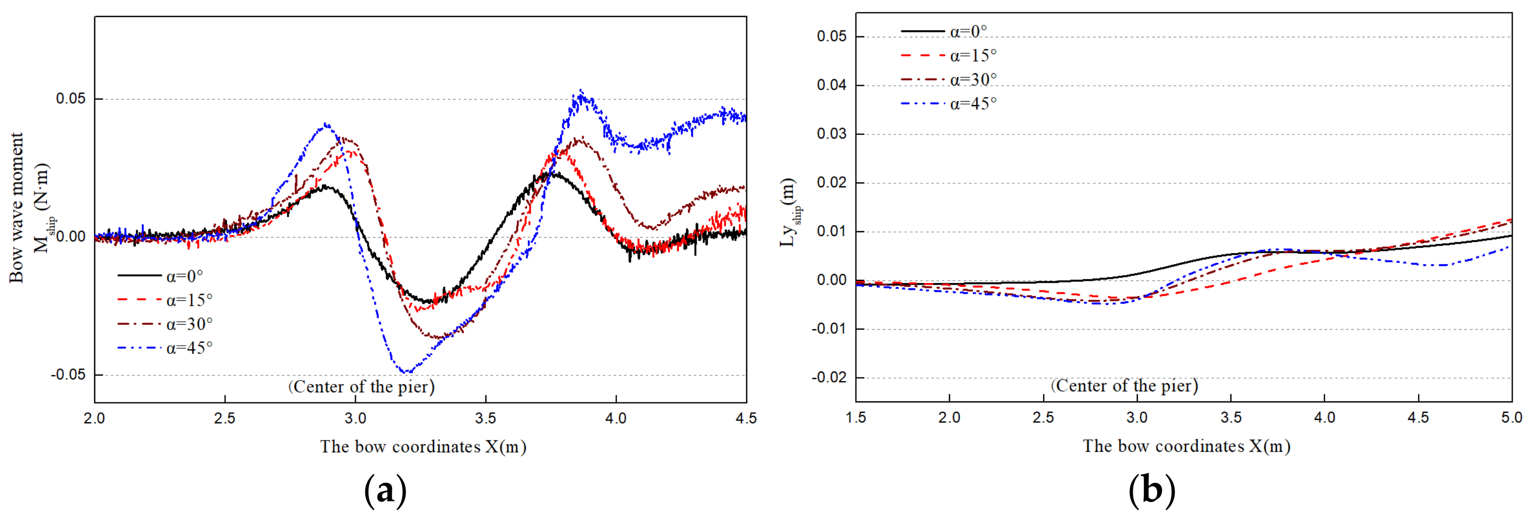
Figure 31a,b show the schematic of the bow roll moment and the position of the center of gravity of the ship passing through the upstream side of the bridge pier, respectively. The peak of the bow roll moment was calculated and is listed in Table 3. As shown, the change in the position of the center of gravity is relatively small when the ship passes through the upstream side of the pier, after the change in the flow angle of attack of the pier, and only has an clear influence on the peak of the ship’s roll moment. When the ship is upstream of the bridge pier, the position of the center of gravity tends to be close to the bridge pier, but is largely unaffected by the change in the flow angle of attack. With the increase in α from 0° to 45°, the range of the positive water pressure on the upstream side of the pier increases, and the water pressure on the bow increases when the ship approaches upstream of the pier, and the first positive peak value of the bow roll moment increases accordingly. When the bow reaches the downstream of the pier, the negative water pressure exerted on the bow and the positive water pressure exerted on the stern in front of the pier both increase with α; thereby, increasing the negative peak value of the bow roll moment. The ‘bulge’ in the center of gravity position curve becomes more evident with the increase in α. After the stern moves to the vortex region of the pier, the negative water pressure of the stern vortex increases with the increase in α, the second positive peak value of the bow roll moment also increases, and the ship turns counterclockwise and keeps a forward attitude. As listed in Table 3, when the flow angle of attack is changed from 0° to 15°, the positive peak increments of bow roll moments I and II are 0.013 and 0.0081 N·m, respectively, which are greater than the increments of 0.0045 and 0.0041 N·m when the flow angle of attack is changed from 15° to 30°. The results indicate that the change in the flow angle of attack of the round-ended pier under 15° has the greatest effect on the ship stress, and the change in the flow angle of attack from 15° to 45° has a relatively stable effect on the ship stress. Generally, although the position of the ship’s center of gravity on the upstream side of the pier tends to be close to the pier in the early stage, the ship’s deviation is less affected by the impact angle of the pier, and the ship’s attitude is relatively stable.
4.5.2. Influence of Flow Angle of Attack on Ships Sailing on the Back Side of a Round-Ended Pier
This section presents the simulation process of a ship passing through the back flow side of a bridge pier with different flow angles of attack; the other parameters are the same as those described in Section 4.5.1.
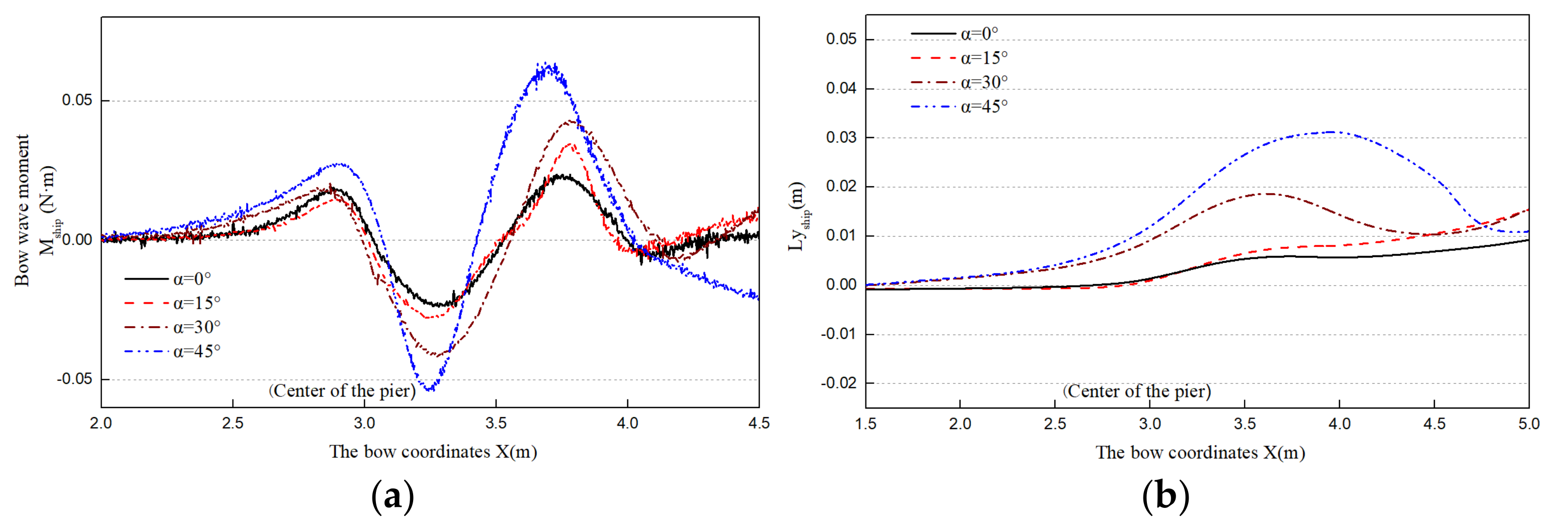
Figure 32a shows a schematic of the bow roll moment of a ship passing through the back flow side of a bridge pier. The peak value of the bow roll moment was calculated and is listed in Table 4. The figure shows that when the ship is passing through the back flow side of the pier, the pier flow angle of attack has a significant influence on the negative peak value and the second positive peak value of the ship’s bow roll moment. The first positive peak values of each bow roll moment are close; the values are 0.0189, 0.0180, and 0.0190 N·m, respectively, when the bow comes to the back flow side of the pier and when the flow angle of attack of the pier are 0°, 15°, and 30°, due to the small difference in the forward water pressure in front of the pier. The negative peak value and the second positive peak value of the bow roll moment increase with the increase in α, particularly when the flow angle of attack is increased from 30° to 45°. The first peak value of the bow roll moment increases by 0.0087 N·m, and the negative peak value and the second positive peak value increase by 0.0539 and 0.0227 N·m, respectively.
Figure 32b shows a schematic of the barycenter position of a ship passing through the back flow side of a bridge pier. As shown, the center of gravity of the ship passing through the bridge area, first moves away from the bridge pier laterally, and then approaches the bridge pier laterally, with the increase in the flow angle of attack. The trajectory of the center of gravity fluctuates more sharply, the ‘bulge’ is more prominent near the bridge pier, and the deviation degree is much greater than when sailing on the upstream side of the pier. Although the ship’s center of gravity keeps a certain transverse distance from the pier to the end, the flow angle of attack of the pier has a significant influence on the attitude of the ship sailing on the back side of the flow.
When the bow enters the negative water pressure area of the stern vortex, the ship experiences a strong forward bow roll as the bow enters the negative water pressure area of the vortex, under the action of the higher negative peak and second positive peak. When the ship leaves the pier, it has a severe negative bow roll. If the rudder is not steered properly or steered in time, the ship will be prone to collision or sweeping bridge pier accidents; hence, the safety of the ship on the back side of the pier is less than that on the upstream side of the pier.
4.5.3. Influence of Transverse Distance between the Ship and Pier on a Ship Sailing in a Skew Bridge Area
This section discusses the influence of different flow angles of attack on a ship passing through the back flow side of a bridge pier under different ship–bridge spacing conditions. The ship’s speed on the opposite shore is 0.566 m/s, and the river velocity is 0.283 m/s.
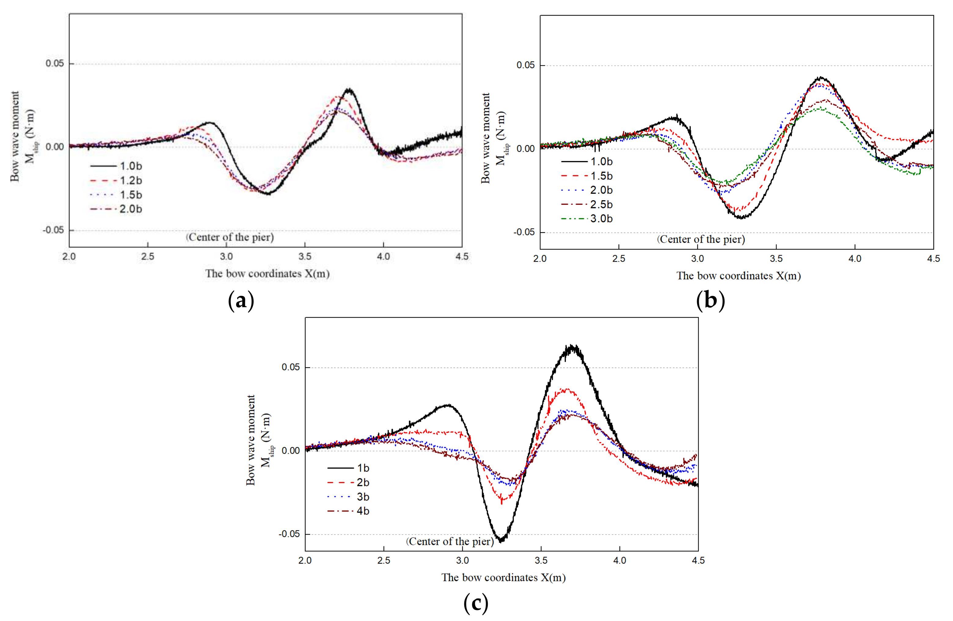
Figure 33 shows a schematic of the ship’s roll moment when passing the back flow side of the bridge pier. The peak of the ship’s roll moment is calculated and listed in Table 5. The chart shows that with the increase in the ship–bridge spacing, the peak values of the bow roll moment acting on the ship along the course decrease, and tend to be stable when the spacing is increased to a certain extent. Taking α = 15° as an example, the positive and negative peak values of the bow roll moment decrease with the increase in the ship–bridge spacing, and when the bridge spacings are 1.5b and 2.0b, the increments in the three peaks of the roll moment (−0.0012, −0.0003, and −0.0009 N·m) tend to be stable. This shows that, when the distance between the ship and bridge is greater than 1.5b, the influence of the water flowing around the pier on ships moving in this area is negligible, and this distance can be used as the safe distance. In addition, the bridge spacing required for the stability of the bow roll moment peak increases with the increase in α. Judging from the fact that the peak increment in the bow roll moment is smaller than the above three increments, it can be concluded that when α = 15°, 30°, and 45°, the safe transverse distances of the bridge are 1.5b, 2.5b, and 3b, respectively, which can be defined as the width of the restricted water area on the back side of the pier.
5. Discussion
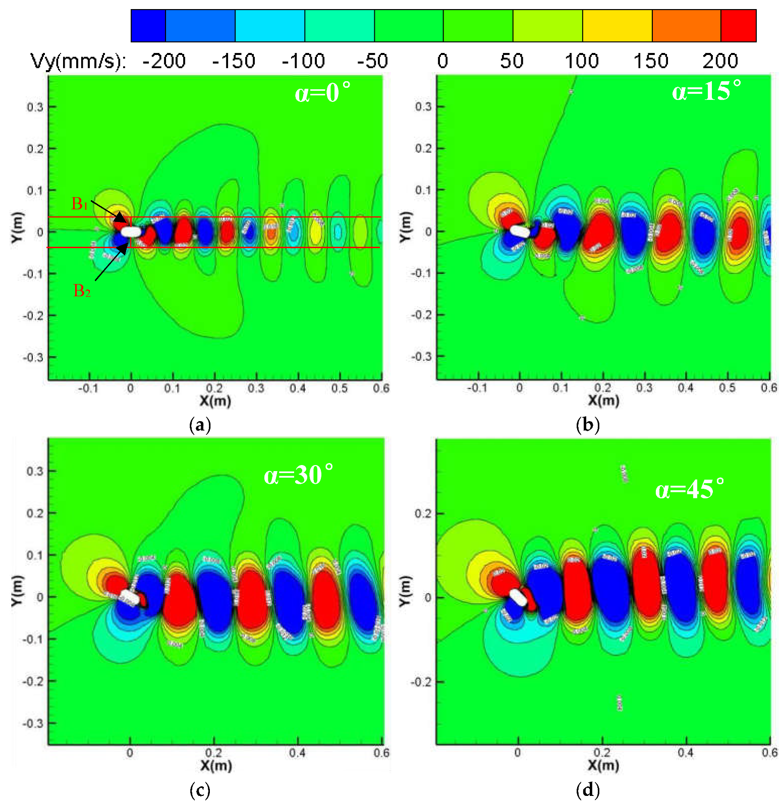
According to China’s current Navigable Standards for Inland Rivers (GB50139-2014), water areas with Vy > 0.3 m/s are unsuitable for ships sailing at low speeds in inland rivers. There is no limit standard for navigable flow conditions in bridge areas, regarding bridge design and other navigable specifications. Hence, based on the limit of the transverse flow velocity in navigable standards for inland rivers, this study defines the water areas B1 and B2 (Figure 34a) with a transverse flow velocity of Vy > 0.3 m/s on both sides of the bridge pier as areas with a significant influence on navigable ships. Based on the flow rate scale calculation, the transverse flow velocity Vy suitable for navigable waters in the PIV test and corresponding numerical model in this study should not exceed 0.02 m/s.
Figure 34a–d show contour maps of the transverse flow velocity around the surface layer of a round-ended bridge pier at different flow angles of attack. The transverse flow rates in dark red and dark blue areas are Vy > 0.02 m/s. Table 6 shows the width of the restricted water area on both sides of the pier. As shown, the scale of the restricted water area on both sides of the bridge pier with α = 0° is approximately 1b in the Y direction. With an increase in the flow angle of attack, B1 and B2 on both sides of the bridge pier increase. When α = 15°, 30°, and 45°, the widths of the restricted water area on the back side of the bridge pier are 1.5b, 1.9b, and 3b, respectively. Notably, the width of the restricted water area at α = 15° and α = 45° is consistent with the simulation results of the spacing between the ship and pier in this study, while the width of the restricted water area at α = 30° slightly deviates, with a difference of only 0.6b. This indicates that the discriminant method of critical lateral velocity may also be suitable for the channel design of skew bridge areas.
6. Conclusions
In this work, a PIV flume test, ship–bridge intersection physical model test, and numerical simulation were used to study the influence of different flow angles of attack of round-ended piers on moving ships. The common barge type and speed in The Xiangjiang River of China were selected as the example parameters. The UDF writing command in Fluent was used to solve for the bow roll moment and center of gravity position of the ship moving in water. Accordingly, the movement of the ship under various conditions was simulated, and the standard for judging the safe space between the ship and bridge, namely the width of the restricted water area, was proposed. The main conclusions are as follows:
- (1)
- The PIV flume test and numerical model test were conducted to study the influence of the flow angle of attack on the flow field and pressure field around a round-ended pier without vessel. The results showed that the fluctuation period of the downstream transverse velocity of the round-ended pier is consistent with the trailing vortex shedding period of the flow around the pier. This period is prolonged with the increase in the flow angle of attack of the pier, but the trailing vortex shedding period tends to be stable at α ≥ 15°. The trailing vortex shedding periods of α = 0°, 15°, 30°, and 45° are 0.8, 1.4, 1.5, and 1.6 s, respectively. Due to the water-blocking effect of the round-ended pier, a positive water pressure area is generated in front of the pier, and this area swings back and forth to the left and right banks when the flow angle of attack α ≥ 30°. A negative water pressure area is generated downstream of the boundary layer separation point of the flow around both sides of the pier, and the pressure area is different on both sides of the pier with the increase in the flow angle of attack. The negative water pressure area of the trailing vortex on the back flow side of the pier is larger than that on the upstream side, and the negative water pressure area generated by the shedding vortex system shifts to the back flow side of the pier with the increase in α.
- (2)
- The accuracy of the numerical simulation results of the ship–bridge intersection was verified based on the ship–bridge intersection model test. The process of the ship drifting through the bridge pier in the channel with a flow rate of 0.283 m/s was deduced by numerical simulation, when the ship–bridge transverse spacing was 1b. The results showed that the ship will be affected by three continuous fluctuation peaks of the bow roll moment, and the ship will experience a change in the bow roll moment direction, from ‘positive’ to ‘negative’ and then from ‘negative’ to ‘positive’. Moreover, the center of gravity position trajectory presents a ‘straw hat’ shape, and the ship will then maintain its attitude, to leave the bridge area.
- (3)
- Through a numerical simulation, the process of a ship passing both sides of the pier with different flow angles of attack at a speed of 0.566 m/s and ship–bridge spacing of 1b was deduced, and the change laws of the bow roll moment and the position of the center of gravity were analyzed. The results showed that the first positive peak value and the second positive peak value of the bow roll moment decrease with the increase in α when the transverse spacing between the ship and pier is constant, and the ship’s attitude is stable. When the ship moves from the back flow side of the bridge pier, although the increase in α has little influence on the overall positive peak value of the bow roll moment, the changes in the negative peak value and second positive peak value are significant, the ship’s navigation attitude is unstable, and the ship has a risk of colliding with the bridge pier and sweeping.
- (4)
- The width of the area that has a significant influence on navigable ships, judged by the hydrodynamic action of the ship on the skew bridge area, is the same as the result judged from the transverse velocity. For the ship class referred to in this study, it is reasonable to take the range of the transverse velocity limit of 0.3 m/s in the bridge area as the area having a significant influence on navigable ships. Combined with the analysis of the impact of the flow angle of attack, this study provides a reference for the width of channel design in skew bridge areas.
Author Contributions
Conceptualization, A.L., G.Z. and X.L.; methodology, A.L., G.Z., X.L. and J.Z.; software, A.L., Y.Y., X.Z. and H.M.; validation, A.L., X.Z. and H.M.; formal analysis, A.L.; investigation, J.Z.; resources, G.Z. and X.L.; data curation, A.L., Y.Y. and X.L.; writing—original draft preparation, A.L.; writing—review and editing, G.Z., X.L. and Y.Y.; visualization, A.L.; supervision, G.Z. and X.L.; project administration, X.L.; funding acquisition, G.Z. and X.L. All authors have read and agreed to the published version of the manuscript.
Funding
This research was funded by the National Natural Science Foundation of China, grant number 51879227.
Institutional Review Board Statement
Not applicable.
Informed Consent Statement
Informed consent was obtained from all subjects involved in the study.
Data Availability Statement
All data, models, or code generated or used during the study are available from the corresponding author by request.
Conflicts of Interest
The authors declare that they have no known competing financial interest or personal relationships that could have appeared to influence the work reported in this paper.
References
- Salaheldin, T.M.; Imran, J.; Chaudhry, M.H. Numerical modeling of three-dimensional flow field around circular piers. J. Hydraul. Eng. 2004, 130, 91–100. [Google Scholar] [CrossRef]
- Vijayasree, B.A.; Eldho, T.I.; Mazumder, B.S. Turbulence statistics of flow causing scour around circular and oblong piers. J. Hydraul. Res. 2020, 58, 673–686. [Google Scholar] [CrossRef]
- Melville, B.W. Local Scour at Bridge Sites. Ph.D. Thesis, University of Auckland, Auckland, New Zealand, 1975. [Google Scholar]
- Kumar, A.; Kothyari, U.; Ranga, R.; Kittur, G. Flow structure and scour around circular compound bridge piers—A review. J. Hydro-Environ. Res. 2012, 6, 251–265. [Google Scholar] [CrossRef]
- Beheshti, A.A.; Ataie-Ashtiani, B. Scour Hole Influence on Turbulent Flow Field around Complex Bridge Piers. Flow Turbul. Combust. 2016, 97, 451–474. [Google Scholar] [CrossRef]
- Ulrich, J.; Michael, M. Flow around a scoured bridge pier: A stereoscopic PIV analysis. Exp. Fluids 2020, 61, 251–265. [Google Scholar] [CrossRef]
- Chang, W.Y.; Constantinescu, G.; Lien, H.C.; Tsai, W.F.; Lai, J.S.; Loh, C.H. Flow Structure around Bridge Piers of Varying Geometrical Complexity. J. Hydraul. Eng. 2013, 139, 812–826. [Google Scholar] [CrossRef]
- Aly, A.M.; Dougherty, E. Bridge pier geometry effects on local scour potential: A comparative study. Ocean Eng. 2021, 234, 109326. [Google Scholar] [CrossRef]
- Link, O.; Henríquez, S.; Ettmer, B. Physical scale modelling of scour around bridge piers. J. Hydraul. Res. 2019, 57, 227–237. [Google Scholar] [CrossRef]
- Al-Saffar, M. The Influence of Dimensional and Dimensionless Parameters on the Dynamics of the Horseshoe Vortex Upstream of a Circular Cylinder. Ph.D. Thesis, University of Sheffield, Sheffield, UK, 2016. [Google Scholar]
- Chakrabarti, S.K.; McBride, M. Model tests on current forces on a large bridge pier near an existing pier. J. Shore Mech. Arct. Eng. 2005, 127, 212–219. [Google Scholar] [CrossRef]
- Daichin; Lee, S.J. Flow structure of the wake behind an elliptic cylinder close to a free surface. KSME Int. J. 2001, 15, 1784–1793. [Google Scholar] [CrossRef]
- Gautam, P.; Eldho, T.I.; Mazumder, B.S.; Behera, M.R. Experimental study of flow and turbulence characteristics around simple and complex piers using PIV. Exp. Therm. Fluid Sci. 2019, 100, 193–206. [Google Scholar] [CrossRef]
- Carnacina, L.; Leonardi, N.; Pagliara, S. Characteristics of Flow Structure around Cylindrical Bridge Piers in Pressure-Flow Conditions. Water 2019, 11, 2240. [Google Scholar] [CrossRef] [Green Version]
- Paul, I.; Prakash, K.A.; Vengadesan, S. Numerical analysis of laminar fluid flow characteristics past an elliptic cylinder. Int. J. Numer. Methods Heat Fluid Flow 2014, 24, 1570–1594. [Google Scholar] [CrossRef]
- Shi, X.; Alam, M.; Bai, H. Wakes of elliptical cylinders at low Reynolds number. Int. J. Heat Fluid Flow 2020, 82, 108553. [Google Scholar] [CrossRef]
- Zhang, C.; Zou, Z.; Wang, H.M. Numerical prediction of the unsteady hydrodynamic interaction between a ship and a bridge pier. Chin. J. Hydrodyn. 2012, 27, 359–364. (In Chinese) [Google Scholar]
- Tuck, E.O.; Newman, J.N. Hydrodynamic interactions between ships. In Proceedings of the Symposium on Naval Hydrodynamics, Pap and Discuss, Cambridge, UK, 24–28 June 1977. [Google Scholar]
- Liu, X.P.; Qian, D.Y.; Fang, S.S.; Zhang, Y. Study on the width of turbulent area around pier with ship impact. Appl. Mech. Mater. 2012, 137, 186–191. [Google Scholar] [CrossRef]
- Wang, H.Z.; Zou, Z.J. Numerical prediction of hydrodynamic forces on a ship passing through a lock with different configurations. J. Hydrodyn. 2014, 26, 1–9. [Google Scholar] [CrossRef]
- Li, L.; Yuan, Z.M.; Ji, C.; Li, M.X.; Gao, Y. Investigation on the unsteady hydrodynamic loads of ship passing by bridge piers by a 3-D boundary element method. Eng. Anal. Bound. Elem. 2018, 94, 122–133. [Google Scholar] [CrossRef] [Green Version]
- Geng, Y.F.; Guo, H.Q.; Ke, X. The flow characteristics around bridge piers under the impact of a ship. J. Hydrodyn. 2020, 32, 1165–1177. [Google Scholar] [CrossRef]
- GB50139-2014. Navigation Standards for Inland Rivers; Planning Publishing Press: Beijing, China, 2014. [Google Scholar]
- TB10002-2017. Code for Design of Railway Bridges and Culverts; Railway Publishing House: Beijing, China, 2017. [Google Scholar]
Figure 1.
Schematic of pier section dimensions.

Figure 2.
Model test layout.

Figure 3.
Schematic of the test instrument layout: (a) Double exposure camera layout; (b) Schematic of laser emitter placement; (c) ADV test frame; (d) ADV measuring probe.
Figure 3.
Schematic of the test instrument layout: (a) Double exposure camera layout; (b) Schematic of laser emitter placement; (c) ADV test frame; (d) ADV measuring probe.


Figure 4.
Instantaneous velocity vector diagram and flow diagram of the round-ended pier with α = 0: (a) T = 0 s; (b) T = 0.387 s; (c) T = 0.780 s.
Figure 4.
Instantaneous velocity vector diagram and flow diagram of the round-ended pier with α = 0: (a) T = 0 s; (b) T = 0.387 s; (c) T = 0.780 s.


Figure 5.
Schematic of ADV measuring point layout.

Figure 6.
Variation rule of the transverse flow velocity from b1 to b3.

Figure 7.
Instantaneous surface flow diagram of the flow around a single circular ended pier with α = 0°. (a) T = 0 s; (b) T = 0.387 s; (c) T = 0.780 s.
Figure 7.
Instantaneous surface flow diagram of the flow around a single circular ended pier with α = 0°. (a) T = 0 s; (b) T = 0.387 s; (c) T = 0.780 s.

Figure 8.
Instantaneous surface flow diagram of flow around a single circular ended pier with α = 15°. (a) T = 0 s; (b) T = 0.684 s; (c) T = 1.357 s.
Figure 8.
Instantaneous surface flow diagram of flow around a single circular ended pier with α = 15°. (a) T = 0 s; (b) T = 0.684 s; (c) T = 1.357 s.

Figure 9.
Instantaneous surface flow diagram of flow around a single circular ended pier with α = 30°. (a) T = 0 s; (b) T = 0.711 s; (c) T = 1.396 s.
Figure 9.
Instantaneous surface flow diagram of flow around a single circular ended pier with α = 30°. (a) T = 0 s; (b) T = 0.711 s; (c) T = 1.396 s.

Figure 10.
Instantaneous surface flow diagram of flow around a single circular ended pier with α = 45°. (a) T = 0 s; (b) T = 0.783 s; (c) T = 1.592 s.
Figure 10.
Instantaneous surface flow diagram of flow around a single circular ended pier with α = 45°. (a) T = 0 s; (b) T = 0.783 s; (c) T = 1.592 s.

Figure 11.
Transverse velocity duration curves downstream of bridge pier: (a) α = 0°; (b) α = 15°; (c) α = 30°; (d) α = 45°.
Figure 11.
Transverse velocity duration curves downstream of bridge pier: (a) α = 0°; (b) α = 15°; (c) α = 30°; (d) α = 45°.


Figure 12.
Physical model test site and key equipment: (a) Layout; (b) Layout; (c) Ship model; (d) Static torque sensor.
Figure 12.
Physical model test site and key equipment: (a) Layout; (b) Layout; (c) Ship model; (d) Static torque sensor.

Figure 13.
Schematic of a trailing vortex around a pier.

Figure 14.
Change rule of bow roll moment.

Figure 15.
Numerical model computing domain.

Figure 16.
Schematic of 2D numerical model meshing for ship–bridge intersection: (a) Schematic of a subregional grid; (b) Grid near the wall of a ship; (c) Grid near the wall of a round-ended pier.
Figure 16.
Schematic of 2D numerical model meshing for ship–bridge intersection: (a) Schematic of a subregional grid; (b) Grid near the wall of a ship; (c) Grid near the wall of a round-ended pier.

Figure 17.
Diagrams of the flow field around a circular end pier: (a) Physical model test results; (b) Numerical simulation results.
Figure 17.
Diagrams of the flow field around a circular end pier: (a) Physical model test results; (b) Numerical simulation results.

Figure 18.
Schematic of the vorticity field around a circular-ended pier surface: (a) Physical model test results; (b) Numerical simulation results.
Figure 18.
Schematic of the vorticity field around a circular-ended pier surface: (a) Physical model test results; (b) Numerical simulation results.

Figure 19.
Comparison diagrams of the transverse velocity–duration curves between model test and numerical simulation, measured at points: (a) b1; (b) b2; (c) b3.
Figure 19.
Comparison diagrams of the transverse velocity–duration curves between model test and numerical simulation, measured at points: (a) b1; (b) b2; (c) b3.

Figure 20.
CL of flow around a round-ended pier with α = 0°.

Figure 21.
Schematics of the flow pressure distribution around the pier: (a) No ship; (b) Ship bowled up to the pier; (c) Bow moves over the pier; (d) Stern sailing over the pier.
Figure 21.
Schematics of the flow pressure distribution around the pier: (a) No ship; (b) Ship bowled up to the pier; (c) Bow moves over the pier; (d) Stern sailing over the pier.


Figure 22.
Change law of the bow roll moment.

Figure 23.
Diagrams of the flow pressure around a round-ended pier: (a) α = 0°; (b) α = 15°.

Figure 24.
Distribution diagrams of CL flow around a circular-ended pier: (a) α = 0°; (b) α = 15°.

Figure 25.
Vorticity field and pressure field distribution diagrams of the flow around a circular-ended pier: (a) α = 30°, T = 0 s; (b) α = 30°, T = 0.0705 s; (c) α = 45°, T = 0 s; (d) α = 45°, T = 0.0775 s.
Figure 25.
Vorticity field and pressure field distribution diagrams of the flow around a circular-ended pier: (a) α = 30°, T = 0 s; (b) α = 30°, T = 0.0705 s; (c) α = 45°, T = 0 s; (d) α = 45°, T = 0.0775 s.

Figure 26.
Distribution diagrams of CL flow around a circular-ended pier: (a) α = 30°; (b) α = 45°.

Figure 27.
Diagrams of the flow pressure distribution and bow roll moment variation of a ship moving through a circular-ended pier at α = 0°: (a) Variation law of the bow roll moment; (b) Ship bowled up to the pier; (c) Bow moving over the pier; (d) Stern moving over the pier.
Figure 27.
Diagrams of the flow pressure distribution and bow roll moment variation of a ship moving through a circular-ended pier at α = 0°: (a) Variation law of the bow roll moment; (b) Ship bowled up to the pier; (c) Bow moving over the pier; (d) Stern moving over the pier.


Figure 28.
Change diagram of the barycenter position of the moving ship in the area of a circular-ended pier bridge with α = 0°.
Figure 28.
Change diagram of the barycenter position of the moving ship in the area of a circular-ended pier bridge with α = 0°.

Figure 29.
Change laws of the bow roll moment and center of gravity position on both sides of the circular-ended pier α = 30°: (a) Bow roll moment; (b) Center of gravity position.
Figure 29.
Change laws of the bow roll moment and center of gravity position on both sides of the circular-ended pier α = 30°: (a) Bow roll moment; (b) Center of gravity position.

Figure 30.
Diagrams of the water pressure distribution of the ship passing the left and right sides of the round-ended pier with α = 30°: (a) Ship bowled up to the pier; (b) Bow moving past the pier; (c) Stern sailing past the pier.
Figure 30.
Diagrams of the water pressure distribution of the ship passing the left and right sides of the round-ended pier with α = 30°: (a) Ship bowled up to the pier; (b) Bow moving past the pier; (c) Stern sailing past the pier.


Figure 31.
Schematic of the bow roll moment and center of gravity position of a ship passing through a round-ended pier with different flow angles of attack: (a) Bow roll moment; (b) Center of gravity position.
Figure 31.
Schematic of the bow roll moment and center of gravity position of a ship passing through a round-ended pier with different flow angles of attack: (a) Bow roll moment; (b) Center of gravity position.

Figure 32.
Schematic of bow roll moment and center of gravity position of a ship passing a round-ended pier with different flow angles of attack: (a) Bow roll moment; (b) Center of gravity position.
Figure 32.
Schematic of bow roll moment and center of gravity position of a ship passing a round-ended pier with different flow angles of attack: (a) Bow roll moment; (b) Center of gravity position.

Figure 33.
Variation in the bow roll moment of a round-ended pier under different bridge spacings: (a) α = 15°; (b) α = 30°; (c) α = 45°.
Figure 33.
Variation in the bow roll moment of a round-ended pier under different bridge spacings: (a) α = 15°; (b) α = 30°; (c) α = 45°.

Figure 34.
Transverse velocity distribution of flow around a round-ended pier with different flow angles of attack: (a) α = 0°; (b) α = 15°; (c) α = 30°; (d) α = 45°.
Figure 34.
Transverse velocity distribution of flow around a round-ended pier with different flow angles of attack: (a) α = 0°; (b) α = 15°; (c) α = 30°; (d) α = 45°.


Table 1.
Bridge pier flow model test group.
| V = 0.141 m/s | Flow Angle of Attack of Round-Ended Pier (α) | |||
|---|---|---|---|---|
| 0° | 15° | 30° | 45° | |
| PIV/ADV | √ | √ | √ | √ |
Table 2.
Numerical simulation table for ship–bridge intersection in skew bridge area.
| Set Time Category | Pier Section Shape | Driving Area | Transverse Spacing between a Ship and Pier | Flow Angle of Attack of the Pier α |
|---|---|---|---|---|
| Validation group | Circular shape (diameter = 1 m) | / | 1b | / |
| Different flow angles of attack | Rounded shape | (1) The backflow side of the pier (2) The upstream side of the pier | 1b | 0° 15° 30° 45° |
| Distance between different ships and piers | Rounded shape | The backflow side of the pier | 1b, 1.2b, 1.5b, 2b 1b, 1.5b, 2b, 2.5b, 3b 1b, 2b, 3b, 4b | 15° 30° 45° |
Table 3.
Statistical table of bow roll moment peaks.
| Parameter | Flow Angle of Attack (α°) | First Positive Peak (N·m) | The Incremental (N·m) | Negative Peak (N·m) | The Incremental (N·m) | Second Positive Peak (N·m) | The Incremental (N·m) |
|---|---|---|---|---|---|---|---|
| Bow roll moment | 0 | 0.0189 | / | −0.0238 | / | 0.0236 | / |
| 15 | 0.0319 | 0.0130 | −0.0271 | −0.0033 | 0.0317 | 0.0081 | |
| 30 | 0.0364 | 0.0045 | −0.0371 | −0.0100 | 0.0358 | 0.0041 | |
| 45 | 0.0422 | 0.0058 | −0.0495 | −0.0124 | 0.0530 | 0.0172 |
Table 4.
Statistical table of bow roll moment peaks.
| Parameter | Flow Angle of Attack (α°) | First Positive Peak (N·m) | The Incremental (N·m) | Negative Peak (N·m) | The Incremental (N·m) | Second Positive peak (N·m) | The Incremental (N·m) |
|---|---|---|---|---|---|---|---|
| Bow roll moment | 0 | 0.0189 | / | −0.0238 | / | 0.0236 | / |
| 15 | 0.0180 | −0.0009 | −0.0287 | −0.0049 | 0.0353 | 0.0117 | |
| 30 | 0.0190 | 0.0040 | −0.0411 | −0.0124 | 0.0398 | 0.0045 | |
| 45 | 0.0277 | 0.0087 | −0.0539 | −0.0128 | 0.0625 | 0.0227 |
Table 5.
Statistical table of bow roll moment peak values under different bridge spacings.
| Flow Angle of Attack (α°) | Transverse Spacing between Ship and Pier | First Positive Peak (N·m) | The Incremental (N·m) | Negative Peak (N·m) | The Incremental (N·m) | Second Positive Peak (N·m) | The Incremental (N·m) |
|---|---|---|---|---|---|---|---|
| 15 | 1.0b | 0.0150 | / | −0.0287 | / | 0.0353 | / |
| 1.2b | 0.0123 | −0.0027 | −0.0271 | 0.0016 | 0.0302 | −0.0051 | |
| 1.5b | 0.0081 | −0.0042 | −0.0257 | 0.0014 | 0.0240 | −0.0062 | |
| 2.0b | 0.0069 | −0.0012 | −0.0254 | 0.0003 | 0.0231 | −0.0009 | |
| 30 | 1.0b | 0.0190 | / | −0.0411 | / | 0.0398 | / |
| 1.5b | 0.0129 | −0.0061 | −0.0377 | 0.0034 | 0.0396 | −0.0002 | |
| 2.0b | 0.0104 | −0.0025 | −0.0262 | 0.0115 | 0.0383 | −0.0013 | |
| 2.5b | 0.0082 | −0.0010 | −0.0222 | 0.0040 | 0.0282 | −0.0101 | |
| 3.0b | 0.0079 | −0.0003 | −0.0216 | 0.0006 | 0.0253 | −0.0029 | |
| 45 | 1.0b | 0.0277 | / | −0.0539 | / | 0.0625 | / |
| 2.0b | 0.0133 | −0.0144 | −0.0291 | 0.0248 | 0.0383 | −0.0242 | |
| 3.0b | 0.0076 | −0.0057 | −0.0199 | 0.0092 | 0.0244 | −0.0139 | |
| 4.0b | 0.0069 | −0.0007 | −0.0188 | 0.0011 | 0.0242 | −0.0002 |
Table 6.
Navigation limits of the width of the water area on either side of a round-ended pier with different flow angles of attack.
Table 6.
Navigation limits of the width of the water area on either side of a round-ended pier with different flow angles of attack.
| Flow Angle of Attack (α) | 0° | 15° | 30° | 45° |
|---|---|---|---|---|
| Ship on the backflow side of the pier (B1) | 1b | 1.5b | 1.9b | 3b |
| Ship on the upstream side of the pier (B2) | 1b | 1.4b | 2.2b | 2b |
Publisher’s Note: MDPI stays neutral with regard to jurisdictional claims in published maps and institutional affiliations. |
© 2022 by the authors. Licensee MDPI, Basel, Switzerland. This article is an open access article distributed under the terms and conditions of the Creative Commons Attribution (CC BY) license (https://creativecommons.org/licenses/by/4.0/).
Share and Cite
MDPI and ACS Style
Li, A.; Zhang, G.; Liu, X.; Yu, Y.; Zhang, X.; Ma, H.; Zhang, J. Hydrodynamic Characteristics at Intersection Areas of Ship and Bridge Pier with Skew Bridge. Water 2022, 14, 904. https://doi.org/10.3390/w14060904
AMA Style
Li A, Zhang G, Liu X, Yu Y, Zhang X, Ma H, Zhang J. Hydrodynamic Characteristics at Intersection Areas of Ship and Bridge Pier with Skew Bridge. Water. 2022; 14(6):904. https://doi.org/10.3390/w14060904
Chicago/Turabian StyleLi, Anbin, Genguang Zhang, Xiaoping Liu, Yuanhao Yu, Ximin Zhang, Huigang Ma, and Jiaqiang Zhang. 2022. "Hydrodynamic Characteristics at Intersection Areas of Ship and Bridge Pier with Skew Bridge" Water 14, no. 6: 904. https://doi.org/10.3390/w14060904
Note that from the first issue of 2016, this journal uses article numbers instead of page numbers. See further details here.