
Development of Rainfall Intensity, Duration and Frequency Relationship on a Daily and Sub-Daily Basis (Case Study: Yalamlam Area, Saudi Arabia)


Civil Engineering Department, King Saud University, P.O. Box 800, Riyadh 11421, Saudi Arabia
*
Author to whom correspondence should be addressed.
Water 2022, 14(6), 897; https://doi.org/10.3390/w14060897
Submission received: 9 February 2022
/
Revised: 4 March 2022
/
Accepted: 10 March 2022
/
Published: 13 March 2022
(This article belongs to the Section Hydrology)
Abstract
:Realistic runoff estimates are crucial for the accurate design of stormwater drainage systems, particularly in developing urban catchments which are prone to overland flow and street inundation following extreme rainstorms. This paper derives new intensity–duration–frequency (IDF) curves for the Yalamlam area in the Kingdom of Saudi Arabia. These curves were obtained based on daily rainfall measurements and, in some short durations, across the entire study area over 30 years. The study is based on applying two distributions—the Log-Pearson type III and Gumbel—to estimate the average rainfall for the different return periods. The results show that there are slight differences between the Log-Pearson type III distribution and the Gumbel distribution, so the average parameters were used to construct the IDF curve in the Yalamlam area. The maximum daily rainfall was converted into sub-daily intervals using two methods and compared with the observed value. The new ratios were calculated using the converting rainfall from daily to sub-daily. These ratios are recommended for application in the Yalamlam area if there are no short-time-interval data available. The following ratios for 1-day rainfall were proposed: 0.37, 0.40, 0.46, 0.53, 0.61, 0.66, 0.70, 0.76, 0.80, and 0.87 for 10 min, 15 min, 30 min, 1 h, 2 h, 3 h, 4 h, 6 h, 8 h, and 12 h rainfall, respectively. The developed IDF curve for the Yalamlam district was built based on the daily and sub-daily observed data.
1. Introduction
The concept of intensity–duration–frequency (IDF) curves of precipitation is based on city stormwater management and engineering infrastructure design to withstand floods and extreme precipitation events [1].
The IDF curves are commonly used by civil engineers and hydrologists to design hydraulic structures. Initiatives for flood mitigation and flood control systems rely on IDF curves for safe and cost-effective design. Stormwater systems and flood control channels and structures are usually based on IDF curves [2].
The first IDF relationships were established in 1932 [3]. Hirschfield [4] created rainfall contour maps to estimate rainfall design depths for a variety of durations and return periods. Chen [5] created a generalized IDF formula for the United States based on three rainfall depths: 1 h, 10-year rainfall depths; 24 h, 10-year rainfall depths; and 1 h, 100-year rainfall depths. For India, Kothyari and Garde [6] showed a relationship between rainfall intensity and 24 h and 2-year rainfall depths. Ghiaei et al. [7] used L-moments and artificial neural networks to assess rainfall intensity–duration–return period data in the Eastern Black Sea Region. They retrieved the governing equations for computation of intensities of 2-, 5-, 25-, 50-, 100-, 250-, and 500-year return periods based on the distribution functions (T). Then, using data on the highest quantity of rainfall at various periods, T values for various rainfall intensities were calculated. In two climatic areas in Canada and South Korea, Yeo et al. [8] examined three fitting approaches for scaling the GEV distribution function in terms of their ability to temporally downscale the daily annual maximum precipitation to be employed in the building of IDF curves. Kristvik et al. [9] used scale invariance to downscale the distribution of severe precipitation in three Norwegian cities from daily to sub-daily timeframes. They used this information to create local-scale intensity–duration–frequency (IDF) curves for future rainfall. Schardong et al. [10] built IDF curves in both gauged and ungauged areas under varied climate conditions using a web-based tool.
Aldosari et al. [11] modified the IDF curves in Kuwait as part of attempts to manage recent flash floods in the country’s metropolitan areas. They contended that Kuwait’s existing IDF curves are inappropriate because they were created roughly three decades ago and do not correctly represent the country’s current rainfall patterns. They compared the revised and previous IDF functions, which revealed increased intensities for the majority of return periods with short durations. Almheiri et al. [12] studied the impact of the cloud-seeding operations that began in 2010 on Sharjah’s IDF curves in the United Arab Emirates. Hourly rainfall data from three stations, Sharjah Airport, Al Dhaid, and Mleiha, spanning the years 2010 to 2020, were used. The developed IDF curves showed an apparent increase in rainfall intensities after implementing the cloud-seeding missions.
In Saudi Arabia, Al-Shaikh [13] suggested dividing Saudi Arabia into six zones to evaluate rainfall data using depth–duration–frequency (DDF) relations. Al-Hassoun [14] presented a rainfall analysis of IDF curves in the Riyadh area using the Gumbel and Log-Pearson type III methods. He noticed no difference in results between the two methods which might be because of the small rainfall variations in the Riyadh region.
Elsebaie [15] generated IDF equations in both the Najran and Hafr-Albatin regions using two distribution methods of the Gumbel and Log-Pearson type III distributions with durations ranging from 10 to 1440 min and return periods ranging from 2 to 100 years. The findings were slightly superior to those obtained from the Log-Pearson III distribution concerning the Gumbel distribution process.
Al-Anazil and Elsebaie [16] established an IDF curve in the Kingdom of Saudi Arabia (KSA) for Abha city. Based on 34 years of results, IDF curves are obtained for eight different durations (10, 20, 30, 60, 120, 180, 360 and 720 min) and six frequency intervals (2, 5, 10, 25, 50 and 100 years). Three frequency distributions have been used, namely: distributions Gumbel, log normal, and Log-Pearson Type III. It was shown that there were minor variations between the three methods obtained from the results.
Ewea et al. [2] developed IDF models and curves to predict rainfall levels for different durations and return times in the Makkah Al Mukarramah area. A consultancy study [17] is used to develop regional maps of probable maximum precipitation to estimate flood frequency for Jabal Sayid in the Al-Madinah region. The empirical formula for the IDF curve was further tested by Subyani and Al-Amri [18], using the 43-year daily rainfall record of Al-Madinah station (M001). Abdeen et al. [19] looked at the distribution of maximum daily rainfall in Saudi Arabia and found that the log-Pearson type III distribution was the best model.
For the AL-Lith wadis in Saudi Arabia, Elsebaie et al. [20] built IDF curves for a variety of return periods and used Gumbel and Log-Pearson type III distributions to predict the maximum rainfall for different metrological stations with varying return periods and topographical characteristics.
The Gumbel and Log-Pearson type III distributions were applied to estimate the average rainfall depth for the different return periods. This procedure is suitable for estimating discharge while constructing structures for flood control. Many researchers in the hydrology and engineering sectors have developed IDF curves for arid and non-arid regions of the world. For example, Bell [21] and Chen [22] derived IDF formulae for some regions of the US. Koutsoyiannis et al. [23] used an efficient parameterization technique to construct an IDF curve mathematical method. In Vietnam, for monsoon zones, empirical functions and widespread IDF equations have been developed [24]. IDF curves have been updated using rainfall techniques and iso-pluvial maps for unheeded sites in the eastern United States [25]. Regional IDF curves derived from isolation maps of untapped sites in the Sinai region of Northeast Egypt [26]. In Malaysia, IDF curves are used in unguessed areas using data from local weather stations that have been updated for standard deviations [27].
IDF curves must be available in order to properly plan for flash floods and runoff collection. There is a wealth of literature on the construction of IDF curves for various areas using various techniques. However, it has been reported that IDF curves do not cover all areas in Saudi Arabia. The topography of the region varies, so the region must be divided into smaller parts for a more accurate assessment of IDF relationships. Furthermore, most rainfall stations provide daily data; therefore, the sub-hourly data are necessary to establish IDF relationships, and many authors use sub-hourly data instead of daily data.
The purpose of this paper was to build IDF curves to estimate the rainfall intensity in the Yalamlam area of Saudi Arabia. The IDF curves are used as an aid for any engineering project when constructing drainage systems. The curves allow the engineer to make efficient and cost-effective flood control steps.
The purpose of this paper is to develop IDF curves for the Wadi Yalamlam area in Saudi Arabia based on daily and sub-daily basis available rainfall data measured in the station. Additionally, ratios for shorter periods were calculated to use if there is only provided daily rainfall data, which need to be converted to sub-daily for a thorough rainfall study.
2. Study Area
Wadi Yalamlam is located approximately 100 km south of Mecca and 90 km north of Al Lith. It lies between the longitudes 39°50′00′′ and 40°36′00′′ and the latitudes 20°33′00″ and 21°07′00″.
The basin of the Yalamlam Wadi occupies a wide area of some 1665 km2. The basin boundary, situated in the downstream area, is extended to include virtually all of the lower flat area. From the high altitudes of the Hijaz Mountains, near Taif, Wadi Yalamlam starts from the Al Shafa region. This has an annual average rainfall of 140 mm. The wadi has various altitudes, ranging widely from 2600 to 25 m. A general location map and a digital elevation model (DEM) of Wadi Yalamlam are shown in Figure 1. The higher and lower parts of the basin are dominated by incisive natural vegetation. Quaternary deposits and sand dunes, on the other hand, followed by tiny dispersed fragments, greatly alter the granitoid and metamorphosed basaltic slopes, the constituents of the lower part of the wadi [28].
3. Methodology and Data Collection
To find the best fit among some probability distributions, accurate analyses of the IDF curves of extreme rainfall amounts of fixed periods are needed. The average annual rainfall intensity for various durations (or the maximum annual rainfall depth over the specified durations) is determined for any recorded year based on the rainfall measurements. Common design times are 5 min, 10 min, 15 min, 30 min, 1 h, 2 h, 6 h, 12 h and 24 h. To construct the IDF curves, each set of the annual maximum for each frequency must be measured, one for each rainy period. The fundamental objective of any frequency analysis is to determine the function of the distribution of rain intensity over each period of probability.
In order to create the IDF curves, the maximum rainfall for certain durations in each year of the historical dataset must be obtained. Converting the daily rainfall data to sub-daily data is a critical part of analysis in many hydrological research. Many rainfall stations only provide daily rainfall data, which need be translated to sub-daily for a thorough rainfall study. There are several experimental and analytical approaches available for this conversion. The Indian Meteorological Department (IMD) has recommended one of the simplest equations:
where Pt is estimated precipitation depth (mm) for the duration of t hours, P24 is depth of daily precipitation (mm) and t is duration (h).
Several methodologies have been utilized in previous research to generate sub-daily data from daily rainfall data, and the rainfall depth-to-duration ratio may be derived using a variety of methods:
- -
- Method A
Wheater et al. [29] used daily rainfall data in the southwestern area of Saudi Arabia to calculate ratios for shorter periods. The rainfall data came primarily from short-duration storm episodes that occurred throughout the day. Wheatear et al. suggested adopting the following ratios of 1-day rainfall to 10 min, 30 min, 1 h, 2 h, and 6 h rainfall: 0.33, 0.56, 0.68, 0.79, and 0.92, respectively.
- -
- Method B
Al-Hassoun [14] developed rainfall depth–duration relationships for the Riyadh region of Saudi Arabia. He proposed the following one-day rainfall to 15 min, 30 min, 1 h, 2 h, 3 h, 4 h, 6 h, 8 h, 12 h rainfall ratios: 0.44, 0.5, 0.56, 0.64, 0.69, 0.72, 078, 0.82, and 0.88, respectively.
Method (A) was applied in the southwest of Saudi Arabia, which is the same region for the current study area. The hydrological characteristics for that region are more or less the same. However, due to the limited data used, which was only six years (1983–1988), as well as this method was presented more than three decades, it did not make up for the climate changes which had happened during the preceding 30 years of the study; therefore, significant variations between the current study and Method (A) are to be expected. Method (B) was developed based on daily rainfall measurements and some short durations spanning 30 years (1963–1994), and this is considered good record. Although their study area was far from the current study area, the results of that method (B) are closer to the current results.
In this study, various statistical distributions, including the Gumbel, generalized extreme value (GEV), Gamma, Normal, and Log-Pearson Type III (LPT III), have been investigated for the creation of IDF curves in the wadi. According to the results, LPT III and Gumbel best suit the data. Rainfall data have been collected from the Ministry of Agriculture, Water and Environment for the J204 station.
The Log-Pearson type III distribution and the Gamble distribution were selected because they show the best fit of the dataset, as shown in the Results section. Estimate rainfall in millimeters and its intensity in mm/h have been calculated for different return periods and durations.
The following equation gives the frequency precipitation PT (in mm) for each duration with a set return time T (in year) for the Gamble distribution.
where K is Gumbel frequency factor given by:
where Pave is the average of the maximum precipitation corresponding to a specific duration.
PT = Pave + KS
In utilizing Gumbel’s distribution, the arithmetic average in Equation (2) is used:
where Pi is the individual extreme value of rainfall and n is the number of events or years of record. The standard deviation is calculated by Equation (5) computed using the following relation:
where S is the standard deviation of P data. The frequency factor (K), which is a function of the sample size and the return period. The rainfall intensity, I (in mm/h) for return period T is obtained from
where Td is durations in hours.
A typical description of the yearly rainfall frequency is the maximum annual sequence which comprises of the highest values in every year. The definition of peak-over threshold is an alternative information format for rainfall frequency studies, which consists of all precipitation amounts exceeding the specified thresholds selected for distinct times. In practice, because of its simpler form, the annual maximum number technique is utilized more often [30].
The simplified expression for this latter distribution is given below for the frequency of precipitation obtained using Log-Pearson type III:
where P*T, P*ave and S* are as defined previously but based on the logarithmically transformed Pi values, i.e., P* of Equation (7). KT is the Pearson frequency factor which depends on return period (T) and skewness coefficient (Cs).
The skewness coefficient, Cs, is required to compute the frequency factor for this distribution. The skewness coefficient was computed by Equation (11) [31,32].
In many hydrological sources, KT values can be determined from tables [31]. The frequency factor KT for the Log-Pearson type III distribution may be extracted by knowing the coefficient of skewness and the recurrence period. The solution antilog in Equation (8) provides the projected extreme value for the return time.
- -
- IDF formula development
The IDF equations reflect the correlations between the intensity of rainfall, duration, and return period. The IDF equation can be written as
where I = intensity of rainfall (mm/h); T = return period (years); t = duration of rainfall (minutes); and a, b, and c are parameters. The parameters are generated from area characteristics and precipitation data using logarithmic relationships and are dependent on the location, shape, and size of the area. Logarithmic function can be applied:
where K = aTb , c denotes the straight line’s slope.
Log(I) = log(k) − c log(t)
Parameters of IDF curve are found by flowing steps:
- -
- Determine the natural logarithm for the (K) value obtained from the Gumbel distribution or the Log-Pearson type III distribution, as well as the natural logarithm for the rainfall period T.
- -
- Draw the log (I) values on the y axis and the log(T) values on the x axis for each return periods.
- -
- Using the graphs, we obtained the value of c for all recurrence intervals, and then we used the following equation to find the average (cave) value, by using the following equation:
Short-duration rainfall is critical for small catchments and urban drainage systems. However, due to a shortage of rain-gauging stations for short-duration rainfall, such critical data are frequently unavailable in many regions of the world. In general, manual rain gauges outnumber automated rain gauges, making it difficult to obtain appropriate data on short-duration rainfall values, which are critical for urban hydrology. The study area is an arid region, and it is exposed to flash floods due to rainfall in very short durations. So, taking into account the short duration data, it is very important and very useful to develop an IDF equation for the Yalamlam wadi area. This can be used in water resource management, flash flood mitigation, and for designing storm drainage systems that use the short rainfall duration to define the design storm. Additionally, the updated and developed ratios can be used later when there is only daily rainfall data available or a shortage in getting short duration data in a similar catchment.
4. Results and Discussion
The study of the morphometric analysis of Wadi Yalamlam is mainly based on the tracing of the drainage network using the Digital Elevation Model (DEM) with 30 m resolution. The different parameters are calculated by WMS program and presented in Table 1.
Figure 2 shows the annual maximum daily rainfall depths of the meteorological station. The rainfall depth ranges from 12.6 to 110 mm. The used data in this study were taken from J204 station that coordinated longitude and latitude are 40.32061 and 21.06409, respectively. The statistical characteristics of the yearly maximum daily rainfall for the meteorological station (J-204) is shown in Table 2.
The Chi-square goodness-of-fit and Kolmogorov–Smirnov tests were used to determine which of the distributions should be used to create the appropriate IDF curves. The Chi-square test compares observed data to the empirical distribution to see how well-observed and -predicted the frequencies resulting from hypothesized distributions fit are. Table 3 shows the results obtained by comparing the probability of each distribution, based on observed precipitation data, with the same expected time given by the distributions investigated, and assuming a significance level of =0.05. The K-S test for goodness-of-fit revealed that, the best-fit distribution was the Log-Pearson type III, with the lowest value of K-S being 0.11. The Gumbel had the lowest Chi-square value—2.
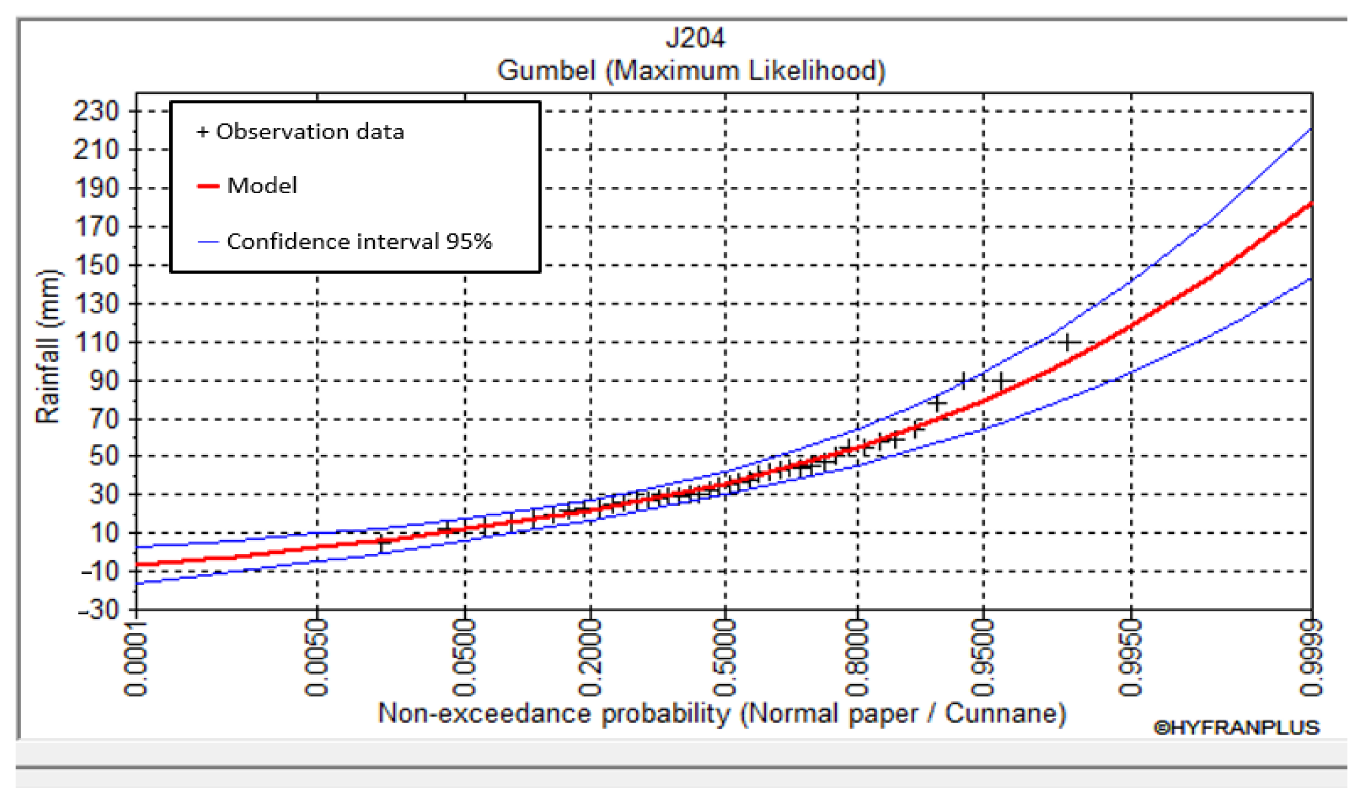
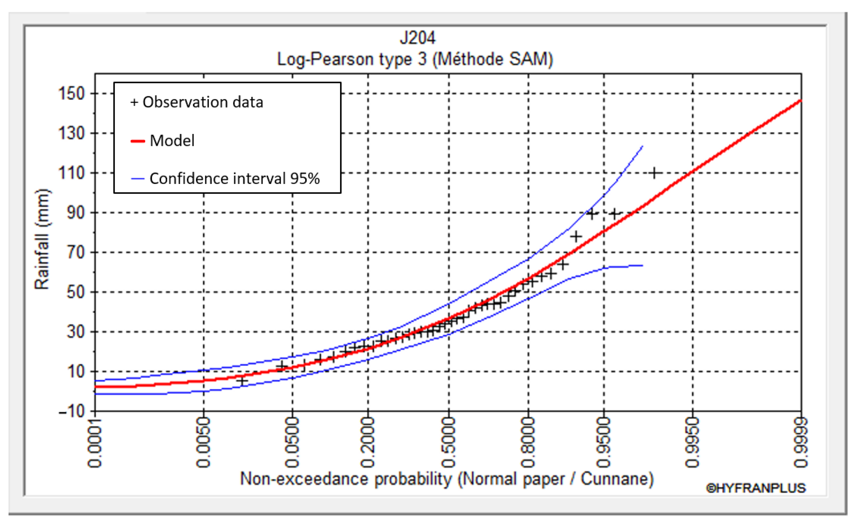
Using the Gamble distribution and the Log-Pearson type III distribution, the maximum rain depth was determined for different periods, and these values are shown in Table 4. A comparison for data obtained from station by using Hyfran software was made between Gumbel and Log-Pearson type III distributions. The distribution of Log-Pearson type III was found to be more suitable for this area, as shown in Figure 3 and Figure 4 for station J204.
Figure 4 shows the non-exceedance probability with 95% confidence intervals for the station. Forecasting return periods of up to 100 years with just 30 years of data available leads to substantially less confidence in the outcomes as the return period grows. In these scenarios, it is clear that the Log-Pearson type III offers a slightly greater range. The confidence interval is relatively broad when the sample size is not too large. As the sample size grows, i.e., more meteorological data are collected over time, the width of the confidence interval around the estimated rainfall quantity will likely be narrow.
Estimated rainfall in mm and its intensity in mm/h were calculated for different return periods and durations using two techniques (Gumbel and Log-Pearson Type III). Table 3 indicates the maximum depth of rainfall for various return periods. It has been shown that there are minor differences between the findings from the two methods, where the method obtained by Log-Pearson III provides slightly greater precision than the Gumbel distribution.
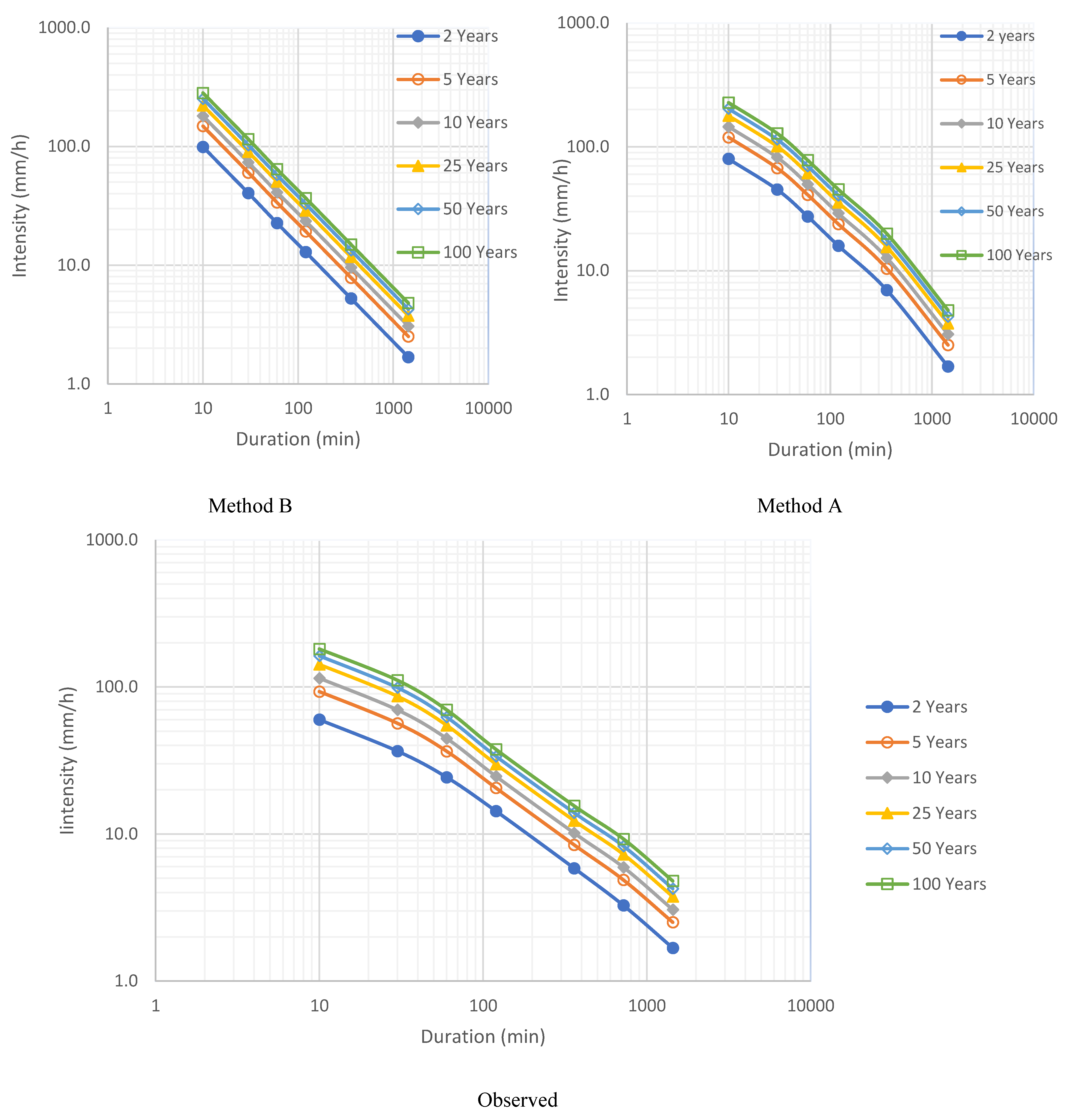
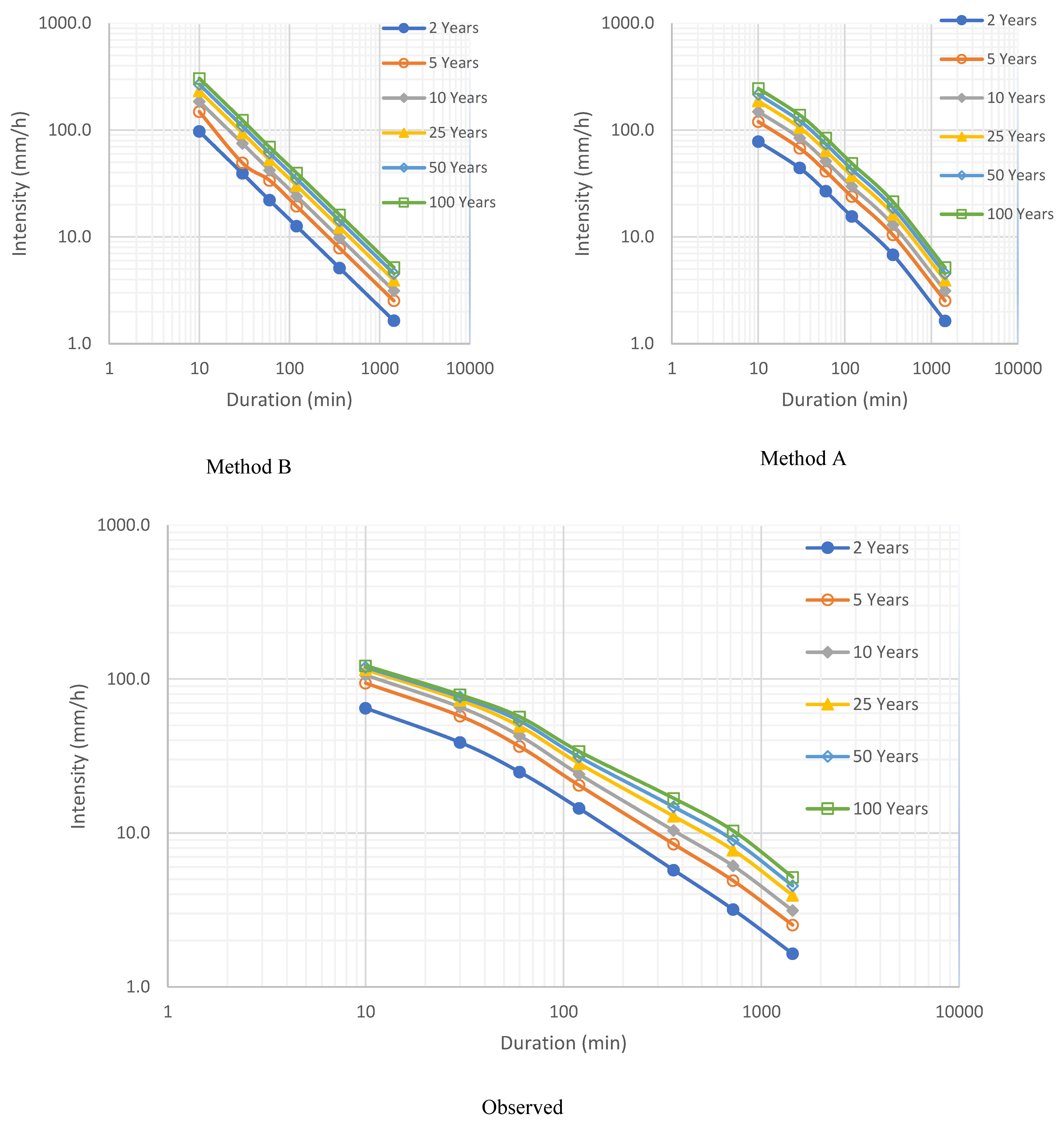
For this area, IDF curves are developed based on Log-Pearson type III and Gumbel distributions because they are more fitting of the available data, as seen in Table 3 and Figure 3 and Figure 4. IDF curves with different return periods of different methods using Gumbel distribution are presented in Figure 5, while IDF curves using Log-Pearson type III distribution are presented in Figure 6. It is noticeable from the figures that the rainfall intensity increases as the return period increases and the intensity decreases as the duration increases for the same return period and all return periods.
Rainfall intensities are related to great differences across the region. Method (A) has the highest intensities for a given duration when using historical data of the southwestern region, while Method (B) is less precise than Method (A), which uses the historical data of the Riyadh region. To explain the differences between various methods, the IDF curves of return periods 100 and 25 years were plotted by using Gumbel and Log-Pearson type III distributions, as shown in Table 5 and Table 6 and Figure 7 and Figure 8.
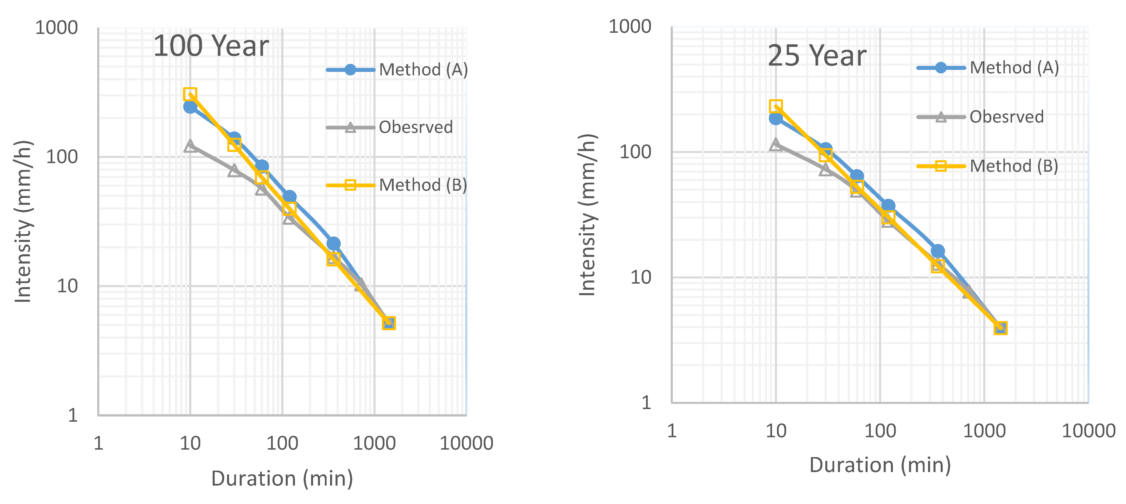
For comparison, the rainfall intensity was plotted with duration at 100-year and 25-year return periods for all methods (A, B, and observed), as shown in Figure 7 and Figure 8.
As can be seen, the rainfall intensity from observed values is the least one by using both distributions Gumbel and Log-Pearson type III. The rainfall intensity using method A is the highest at all rainfall durations except when the duration of rainfall is 10 min, in which case Method B is higher than Method A and the observed value because it uses both distributions (Gumel and Log-Pearson type III). The rainfall intensity from method B and the observed value give similar results from a duration of 120 to 1440 min. The gaps between them increase when the duration is less than 120 min, until they reach their maximum when the duration is 10 min.
In Figure 8, it is clear that there is a deviation in rainfall intensity between the observed and two methods (A,B). This is clear for a rainfall duration less than 100 min when the Log-Pearson type III distribution was applied. On the other hand, this deviation for the same rainfall durations is very small when using Gumbel distribution, as shown in Figure 7. This deviation may be due to one of the reasons mentioned before—either the data record used in Method (A) was too short and did not cover the phenomena of climate change occurring during the current study records, or the hydrological and topographic characteristics of this study area are different compared to previous studies.
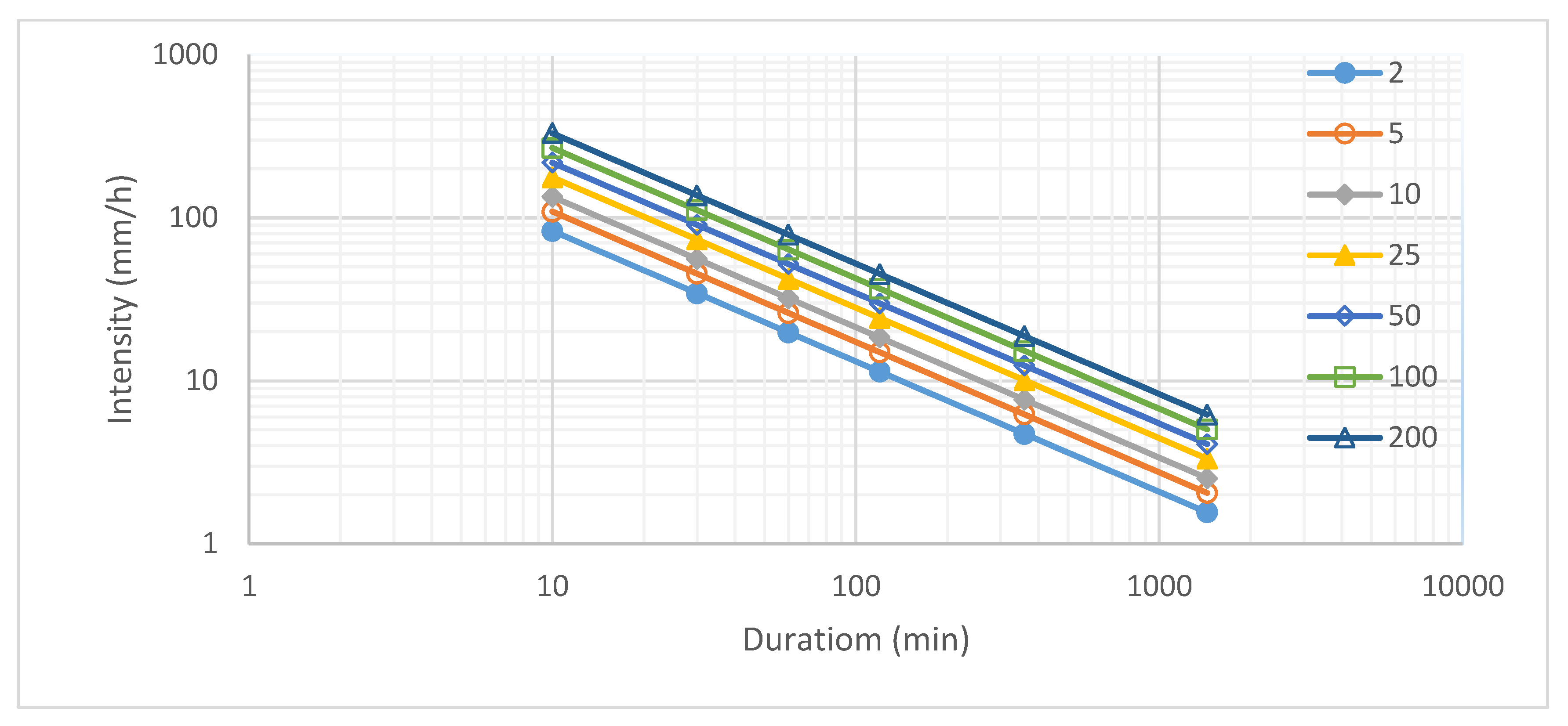
In IDF formula development section, we proposed a method to calculate the parameters of IDF curve using equation (Equation (12)). After carrying out these steps and obtaining the average parameters (a, b and c) using Gumbel and Log-Pearson type III distributions, the final values of parameters a, b, and c are 425, 0.3, and 0.8, respectively. So, for calculating rainfall intensity IT for any design storm with a specified duration td (min) and return time Tr (years) for the Yalamlam area, you can use Equation (15) or Figure 9.
Due to the urgent need to find rainfall values for a short interval (sub-daily) and because most rainfall stations give rain values of the daily readings, so the relationship to convert the daily readings into sub-daily is built. The percentages were calculated for the short intervals of daily values based on Equation (15), as shown in Table 7, which was calculated from the observed data. The ratios are recommending for use in Wadi Yalamem and the nearby areas.
Figure 10 shows compression of the ratio to daily rainfall with duration between Method A, Method B and the ratio calculated from observed values. The ratios from Method A were higher than the ratios from Method B and the calculated ratio. There was a small difference between the ratios from Method B and the calculated ratio.
Although the obtained developed model’s results are close to Method (B), it is favorable to have a unique IDF equation for the current study area—different to the nature of the area which was used in Method (B)—recommended for specific application in the Riyadh region. On the other hand, the current study area was exposed to severe flash flood during the last five years, which caused damage to property and human health; therefore, more intensive studies are recommended in that area to develop a reliable IDF equation which can be used in the storm drainage systems and measure mitigations.
5. Conclusions
The intensity–duration–frequency (iDf) curves are a significant technical resource for hydrologists and engineers engaged in the design of water projects. Historical rainfall intensity records are provided from a major meteorological station (J204) using the best possible distribution methods. Based on results from the probability density function, linked IDF curves of different durations (15, 30, 60, 120, 180, 480, 720, and 1440 min) shall be extracted with the relevant return periods of 2, 5, 10, 25, 50, 100, and 200 years. The Log-Pearson type III and Gumbel distributions were chosen, so they were selected to build the IDF curve because they were more fitting to the available data. The IDF curve equation was developed and the parameters were found so the equation could be used to find the rainfall intensity of different durations and different return periods for the Yalamlam area. The ratios were suggested of 1-day rainfall to 10 min, 15 min, 30 min, 1 h, 2 h, 3 h, 4 h, 6 h, 8 h, and 12 h rainfall ratios: 0,37, 0.40, 0.46, 0.53, 0.61, 0.66, 0.70, 076, 0.80, and 0.87, respectively, and use these ratios in the Yalamlam area if the sub-daily rainfall data were not available.
Further research employing satellite production, i.e., the Global Precipitation Measurement (GPM), is advised to explore and evaluate the veracity of the observed rainfall data, as well as to address the problem of a lack of rainfall stations in the catchment region. As a result, after adding the satellite production, the acquired IDF curves may be adjusted. An appropriate and reliable assessment of IDF curves will enable and assure the planning and optimal design of hydraulic structures, as well as future flood hazard studies, and as a result, disaster risk management will directly benefit from that research.
Author Contributions
Conceptualization, I.H.E.; Formal analysis, A.Q.K. and I.H.E.; Investigation, I.H.E.; Methodology, A.Q.K.; Software, A.Q.K.; Supervision, I.H.E.; Writing—original draft, A.Q.K.; Writing—review and editing, I.H.E. All authors have read and agreed to the published version of the manuscript.
Funding
This research was funded by the National Plan for Science, Technology and Innovation (MAARIFAH), King Abdulaziz City for Science and Technology, Kingdom of Saudi Arabia, Award Number (13-WAT1027-02).
Institutional Review Board Statement
Not applicable.
Informed Consent Statement
Not applicable.
Acknowledgments
The authors extend their sincere appreciations to the National Plan for Science, Technology and Innovation (NPST)-King Saud University for funding the Research Project (13-WAT1027-02).
Conflicts of Interest
The authors declare no conflict of interest.
References
- Wayal, A.S.; Menon, K. Intensity–Duration–Frequency Curves and Regionalization. Int. J. Innov. Res. Adv. Eng. 2014, 1, 28–32. [Google Scholar]
- Ewea, H.A.; Elfeki, A.M.; Bahrawi, J.A.; Al-Amri, N.S. Modeling of IDF curves for stormwater design in Makkah Al Mukarramah region, The Kingdom of Saudi Arabia. Open Geosci. 2018, 10, 954–969. [Google Scholar] [CrossRef]
- Bernard, M.M. Formulas for rainfall intensities of long duration. Trans. Am. Soc. Civ. Eng. 1932, 96. [Google Scholar] [CrossRef]
- Hershfield, D.M. Estimating the Probable Maximum Precipitation. J. Hydraul. Div. 1961, 87, 99–116. [Google Scholar] [CrossRef]
- Cheng, L.; AghaKouchak, A. Nonstationary Precipitation Intensity-Duration-Frequency Curves for Infrastructure Design in a Changing Climate. Sci. Rep. 2015, 4, 7093. [Google Scholar] [CrossRef] [PubMed] [Green Version]
- Kothyari, U.C.; Garde, R.J. Rainfall Intensity-Duration-Frequency Formula for India. J. Hydraul. Eng. 1992, 118, 323–336. [Google Scholar] [CrossRef]
- Ghiaei, F.; Kankal, M.; Anilan, T.; Yuksek, O. Regional intensity–duration–frequency analysis in the Eastern Black Sea Basin, Turkey, by using L-moments and regression analysis. Arch. Meteorol. Geophys. Bioclimatol. Ser. B 2018, 131, 245–257. [Google Scholar] [CrossRef]
- Yeo, M.-H.; Nguyen, V.-T.-V.; Kpodonu, T.A. Characterizing Extreme Rainfalls and Constructing Confidence Intervals for IDF Curves Using Scaling-GEV Distribution Model. Int. J. Climatol. 2021, 41, 456–468. [Google Scholar] [CrossRef]
- Kristvik, E.; Johannessen, B.G.; Muthanna, T.M. Temporal Downscaling of IDF Curves Applied to Future Performance of Local Stormwater Measures. Sustainability 2019, 11, 1231. [Google Scholar] [CrossRef] [Green Version]
- Schardong, A.; Simonovic, S.P.; Gaur, A.; Sandink, D. Web-Based Tool for the Development of Intensity Duration Frequency Curves under Changing Climate at Gauged and Ungauged Locations. Water 2020, 12, 1243. [Google Scholar] [CrossRef]
- Aldosari, D.; Almedeij, J.; Alsumaiei, A.A. Update of Intensity–Duration–Frequency Curves for Kuwait Due to Extreme Flash Floods. Environ. Ecol. Stat. 2020, 27, 491–507. [Google Scholar] [CrossRef]
- Almheiri, K.B.; Rustum, R.; Wright, G.; Adeloye, A.J. Study of Impact of Cloud-Seeding on Intensity-Duration-Frequency (IDF) Curves of Sharjah City, the United Arab Emirates. Water 2021, 13, 3363. [Google Scholar] [CrossRef]
- Al-Shaikh, A. Rainfall Frequency Studies for Saudi Arabia. Master’s Thesis, Civil Engineering Department, King Saud University, Riyadh, Saudi Arabia, 1985. [Google Scholar]
- AlHassoun, S.A. Developing an empirical formulae to estimate rainfall intensity in Riyadh region. J. King Saud Univ. Eng. Sci. 2011, 23, 81–88. [Google Scholar] [CrossRef] [Green Version]
- Elsebaie, I.H. Developing rainfall intensity–duration–frequency relationship for two regions in Saudi Arabia. J. King Saud Univ. Eng. Sci. 2012, 24, 131–140. [Google Scholar] [CrossRef] [Green Version]
- Al-anazi, K.K.; El-Sebaie, D.I.H. Development of Intensity-Duration-Frequency Relationships for Abha City in Saudi Arabia. Int. J. Comput. Eng. Res. 2013, 3, 58–65. [Google Scholar]
- Subyani, A.M.; Alahmadi, F. Rainfall-Runoff Modeling in the Al-Madinah Area of Western Saudi Arabia. J. Environ. Hydrol. 2011, 19, 1–13. [Google Scholar]
- Subyani, A.M.; Al-Amri, N.S. IDF curves and daily rainfall generation for Al-Madinah city, western Saudi Arabia. Arab. J. Geosci. 2015, 8, 11107–11119. [Google Scholar] [CrossRef]
- Abdeen, W.M.; Awadallah, A.G.; Hassan, N.A. Investigating regional distribution for maximum daily rainfall in arid regions: Case study in Saudi Arabia. Arab. J. Geosci. 2020, 13, 501. [Google Scholar] [CrossRef]
- Elsebaie, I.H.; El Alfy, M.; Kawara, A.Q. Spatiotemporal Variability of Intensity–Duration–Frequency (IDF) Curves in Arid Areas: Wadi AL-Lith, Saudi Arabia as a Case Study. Hydrology 2021, 9, 6. [Google Scholar] [CrossRef]
- Bell, F.C. Generalized Rainfall-Duration-Frequency Relationships. J. Hydraul. Div. 1969, 95, 311–328. [Google Scholar] [CrossRef]
- Chen, C. Rainfall Intensity-Duration-Frequency Formulas. J. Hydraul. Eng. 1983, 109, 1603–1621. [Google Scholar] [CrossRef]
- Koutsoyiannis, D.; Kozonis, D.; Manetas, A. A mathematical framework for studying rainfall intensity-duration-frequency relationships. J. Hydrol. 1998, 206, 118–135. [Google Scholar] [CrossRef]
- Nhat, L.M.; Tachikawa, Y.; Takara, K. Establishment of Intensity-Duration-Frequency Curves for Precipitation in the Monsoon Area of Vietnam. Annu. Disas. Prev. Res. Inst. Kyoto Univ. 2006, 49, 93–103. [Google Scholar]
- Raiford, J.P.; Aziz, N.M.; Powell, D.N.; Khan, A.A. Rainfall Depth-Duration-Frequency Relationships for South Carolina, North Carolina, and Georgia. Am. J. Environ. Sci. 2007, 3, 78–84. [Google Scholar] [CrossRef]
- El-Sayed, E.A.H. Generation of Rainfall Intensity Duration Frequency Curves for Ungauged Sites. Nile Basin Water Sci. Eng. J. 2011, 4, 112–124. [Google Scholar]
- Liew, S.C.; Raghavan, S.V.; Liong, S.-Y. Development of Intensity-Duration-Frequency curves at ungauged sites: Risk management under changing climate. Geosci. Lett. 2014, 1, 8. [Google Scholar] [CrossRef] [Green Version]
- Aldhebiani, A.Y.; Elhag, M.; Hegazy, A.K.; Galal, H.K.; Mufareh, N.S. Consideration of NDVI thematic changes in density analysis and floristic composition of Wadi Yalamlam, Saudi Arabia. Geosci. Instrum. Methods Data Syst. 2018, 7, 297–306. [Google Scholar] [CrossRef] [Green Version]
- Wheater, H.S.; Laurentis, P.; Hamilton, G.S. Design rainfall characteristics for south-west Saudi Arabia. Proc. Inst. Civ. Eng. 1989, 87, 517–538. [Google Scholar] [CrossRef]
- Borga, M.; Vezzani, C.; Dalla Fontana, G. Regional Rainfall Depth–Duration–Frequency Equations for an Alpine Region. Nat. Hazards 2005, 36, 221–235. [Google Scholar] [CrossRef]
- Chow, V.T. Bibliography: 1) Handbook of Applied Hydrology. Int. Assoc. Sci. Hydrol. Bull. 1965, 10, 82–83. [Google Scholar] [CrossRef]
- Burke, C.B.; Burke, T.T. Storm Drainage Manual. Indiana LTAP 2008. Available online: https://docs.lib.purdue.edu/cgi/viewcontent.cgi?article=1099&context=inltappubs (accessed on 2 September 2019).
- Al-Areeq, A.; Al-Zahrani, M.; Chowdhury, S. Rainfall Intensity–Duration–Frequency (IDF) Curves: Effects of Uncertainty on Flood Protection and Runoff Quantification in Southwestern Saudi Arabia. Arab. J. Sci. Eng. 2021, 46, 10993–11007. [Google Scholar] [CrossRef]
Figure 1.
General location map and digital elevation model (DEM) of Wadi Yalamlam.

Figure 2.
Maximum 24 h rainfall precipitation at J-204 station.

Figure 3.
Gumbel fit of maximum daily rainfall of J204 station.

Figure 4.
Log-Pearson type 3 fit of maximum daily rainfall for J204 station.

Figure 5.
IDF curves by using Gumbel distribution of Yalamlam area (method A, B and observed).

Figure 6.
IDF curves by Log-Pearson type III distribution of Yalamlam area (Methods A, B and observed).
Figure 6.
IDF curves by Log-Pearson type III distribution of Yalamlam area (Methods A, B and observed).

Figure 7.
Comparison of IDF curves between two methods and observed with return periods 100 and 25 years using Gumbel distribution.
Figure 7.
Comparison of IDF curves between two methods and observed with return periods 100 and 25 years using Gumbel distribution.

Figure 8.
Comparison of IDF curves between two methods and observed with return periods 100 and 25 years using Log-Pearson type III distribution.
Figure 8.
Comparison of IDF curves between two methods and observed with return periods 100 and 25 years using Log-Pearson type III distribution.

Figure 9.
IDF curves of the Wadi Yalamlam area.

Figure 10.
Ratio to daily rainfall.


Table 1.
Topographic parameters of Wadi Yalamlam catchment.
| Basin Area (A) | 1665 (km2) |
| Basin Slope (BS) | 0.1308 (m/m) |
| Average Overland Flow (AOFD) | 1.23 (km) |
| Basin lengths (L) | 88.01 (km) |
| Mean Basin elevation (AVEL) | 771.84 (m) |
| Max Flow Distance (MFD) | 110.8 (km) |
| Max Flow Slope (MFS) | 0.0210 (m/m) |
| Centroid stream Distance (CSD) | 68.8 (km) |
Table 2.
Statistical characteristics of the annual maximum daily rainfall of J-204 station.
| Station | J-204 |
|---|---|
| Sample size | 30 |
| Minimum (mm) | 12.6 |
| Maximum (mm) | 110 |
| Median (mm) | 41.6 |
| Mean (mm) | 44.5 |
| Standard deviation | 23.3 |
| Variation coefficient | 0.524 |
| Skewness coefficient | 1.14 |
| Kurtosis coefficient | 3.54 |
Table 3.
Summary of the best-fit distribution of stations.
| Stations | Gumbel | GEV | Gamma | Normal | LPT III | |||||
|---|---|---|---|---|---|---|---|---|---|---|
| Chi-Square | K-S | Chi-Square | K-S | Chi-Square | K-S | Chi-Square | K-S | Chi-Square | K-S | |
| J-204 | 2 | 0.113 | 3.2 | 0.112 | 4.8 | 0.118 | 4.8 | 0.119 | 3.2 | 0.11 |
Note: Bold font in the table shows the minimum K-S and Chi-square values obtained from the data.
Table 4.
The maximum 24 h rainfall depths for different return period of J204 station.
| Return Period (Year) | 2 | 5 | 10 | 25 | 50 | 100 |
| Gumbel (mm) | 40.4 | 60.1 | 73.2 | 89.6 | 102 | 114 |
| Log-Pearson type III | 39.7 | 60.5 | 74.8 | 93.3 | 107 | 121 |
Table 5.
The rainfall intensity of 100- and 25-year return periods using Gumbel distribution.
| Duration (min) | Rainfall Intensity (mm/h) | |||||
|---|---|---|---|---|---|---|
| Return Period of 100-Year | Return Period of 25-Year | |||||
| Method (A) | Method (B) | Observed | Method (A) | Method (B) | Observed | |
| 10 | 224.7 | 282 | 181.2 | 178.2 | 221.4 | 142.2 |
| 30 | 128.6 | 114.8 | 111 | 101 | 90 | 86.4 |
| 60 | 78 | 64.3 | 69.8 | 61.3 | 50.5 | 54.8 |
| 120 | 45.3 | 36.7 | 37.6 | 35.6 | 28.9 | 29.9 |
| 360 | 19.9 | 14.9 | 15.5 | 15.5 | 11.7 | 12.3 |
| 1440 | 4.8 | 4.8 | 4.8 | 3.8 | 3.8 | 3.8 |
Table 6.
The rainfall intensity of 100- and 25-year return periods using Log-Pearson type III distribution.
Table 6.
The rainfall intensity of 100- and 25-year return periods using Log-Pearson type III distribution.
| Duration (min) | Rainfall Intensity (mm/h) | |||||
|---|---|---|---|---|---|---|
| Return Period of 100-Year | Return Period of 25-Year | |||||
| Method (A) | Method (B) | Observed | Method (A) | Method (B) | Observed | |
| 10 | 254.4 | 304.8 | 122.4 | 187.2 | 232.2 | 115.2 |
| 30 | 138.8 | 124 | 79.2 | 105.8 | 94.4 | 73 |
| 60 | 84.3 | 69.4 | 56.9 | 64.2 | 52.9 | 49.4 |
| 120 | 49 | 39.9 | 33.9 | 37.3 | 30.2 | 28.3 |
| 360 | 21.4 | 16.1 | 16.8 | 16.3 | 12.3 | 12.9 |
| 1440 | 5.2 | 5.2 | 5.2 | 3.9 | 3.9 | 3.9 |
Table 7.
Ratio to daily rainfall.
| Duration (h) | 24 h Rainfall (%) |
|---|---|
| 24 | 1.00 |
| 12 | 0.87 |
| 8 | 0.80 |
| 6 | 0.76 |
| 4 | 0.70 |
| 3 | 0.66 |
| 2 | 0.61 |
| 1 | 0.53 |
| 0.5 (30 min) | 0.46 |
| 0.25 (15 min) | 0.40 |
| 0.167 (10 min) | 0.37 |
Publisher’s Note: MDPI stays neutral with regard to jurisdictional claims in published maps and institutional affiliations. |
© 2022 by the authors. Licensee MDPI, Basel, Switzerland. This article is an open access article distributed under the terms and conditions of the Creative Commons Attribution (CC BY) license (https://creativecommons.org/licenses/by/4.0/).
Share and Cite
MDPI and ACS Style
Kawara, A.Q.; Elsebaie, I.H. Development of Rainfall Intensity, Duration and Frequency Relationship on a Daily and Sub-Daily Basis (Case Study: Yalamlam Area, Saudi Arabia). Water 2022, 14, 897. https://doi.org/10.3390/w14060897
AMA Style
Kawara AQ, Elsebaie IH. Development of Rainfall Intensity, Duration and Frequency Relationship on a Daily and Sub-Daily Basis (Case Study: Yalamlam Area, Saudi Arabia). Water. 2022; 14(6):897. https://doi.org/10.3390/w14060897
Chicago/Turabian StyleKawara, Atef Q., and Ibrahim H. Elsebaie. 2022. "Development of Rainfall Intensity, Duration and Frequency Relationship on a Daily and Sub-Daily Basis (Case Study: Yalamlam Area, Saudi Arabia)" Water 14, no. 6: 897. https://doi.org/10.3390/w14060897
Note that from the first issue of 2016, this journal uses article numbers instead of page numbers. See further details here.