
Dynamic Modeling of Crop–Soil Systems to Design Monitoring and Automatic Irrigation Processes: A Review with Worked Examples


1
Department of Electrical and Electronic Engineering, Universidad de los Andes, Bogotá 111711, Colombia
2
Systems, Estimation, Control, and Optimization (SECO), University of Mons, 7000 Mons, Belgium
*
Author to whom correspondence should be addressed.
Water 2022, 14(6), 889; https://doi.org/10.3390/w14060889
Submission received: 28 January 2022
/
Revised: 7 March 2022
/
Accepted: 9 March 2022
/
Published: 12 March 2022
(This article belongs to the Special Issue Research on Irrigation Strategies for Sustainable Water Management)
Abstract
:The smart use of water is a key factor in increasing food production. Over the years, irrigation has relied on historical data and traditional management policies. Control techniques have been exploited to build automatic irrigation systems based on climatic records and weather forecasts. However, climate change and new sources of information motivate better irrigation strategies that might take advantage of the new sources of information in the spectrum of systems and control methodologies in a more systematic way. In this connection, two open questions deserve interest: (i) How can one deal with the space–time variability of soil conditions? (ii) How can one provide robustness to an irrigation system under unexpected environmental change? In this review, the different elements of an automatic control system are described, including the mathematical modeling of the crop–soil systems, instrumentation and actuation, model identification and validation from experimental data, estimation of non-measured variables and sensor fusion, and predictive control based on crop–soil and weather models. An overview of the literature is given, and several specific examples are worked out for illustration purposes.
1. Introduction
The rise of the world population motivates the increase in food production. To achieve this goal, irrigation plays a major role, since 70% of fresh water around the world is used in agriculture [1]. A challenge is to increase production while following a sustainable and efficient strategy [2,3]. Efficient irrigation has a determinant impact on the water footprint of agricultural production, which depends not only on the amount of water that is used, but also on the way it is exploited and on the water sources [4]. On the one hand, sustainability is linked to water scarcity and climate change, since historical climatic data may not be sufficient to determine irrigation strategies. This issue was discussed by [5], where the authors proposed an adaptive irrigation strategy. On the other hand, the design of irrigation systems involves a proper interpretation of the crop–soil system in order to propose an optimal irrigation policy. One of the most relevant open challenges is the management of land heterogeneity related to topography and soil properties [6]. Over the years, the representation of crop–soil dynamics has been addressed with mathematical models, where the cause–effect relations between environmental variables and plant/soil components have been incorporated. These models mainly include mass balance equations, heuristic relationships, and statistical functions. The historical evolution of these models was described by [6,7,8]. Nevertheless, modeling of irrigation systems has traditionally been limited to soil dynamics, neglecting the plants’ interactions and effects [9], which has led to sub-optimal solutions [10]. Consequently, the design of irrigation systems can be enhanced by more comprehensive models that take interactions between the different system compartments into account and by a more systematic use of system and control theory to improve monitoring and predictive control.
This trend in smart farming and precision agriculture has been boosted by the availability of more sources of information, notably, through remote sensing [8,11,12], thus also leading to the use of machine learning [13]. The applications of these tools have led to improvements in production performance, as discussed in [14].
However, there is still room for a full exploitation of system and control methodologies, particularly in this new era of massive data sources, as recently pointed out by [15]. In this latter review article, the authors emphasized two research directions, i.e., minimal resource usage and the exploitation of current technology to build better management systems. The open challenges include the resource allocation problem, control-oriented modeling, and sensor and actuator placement.
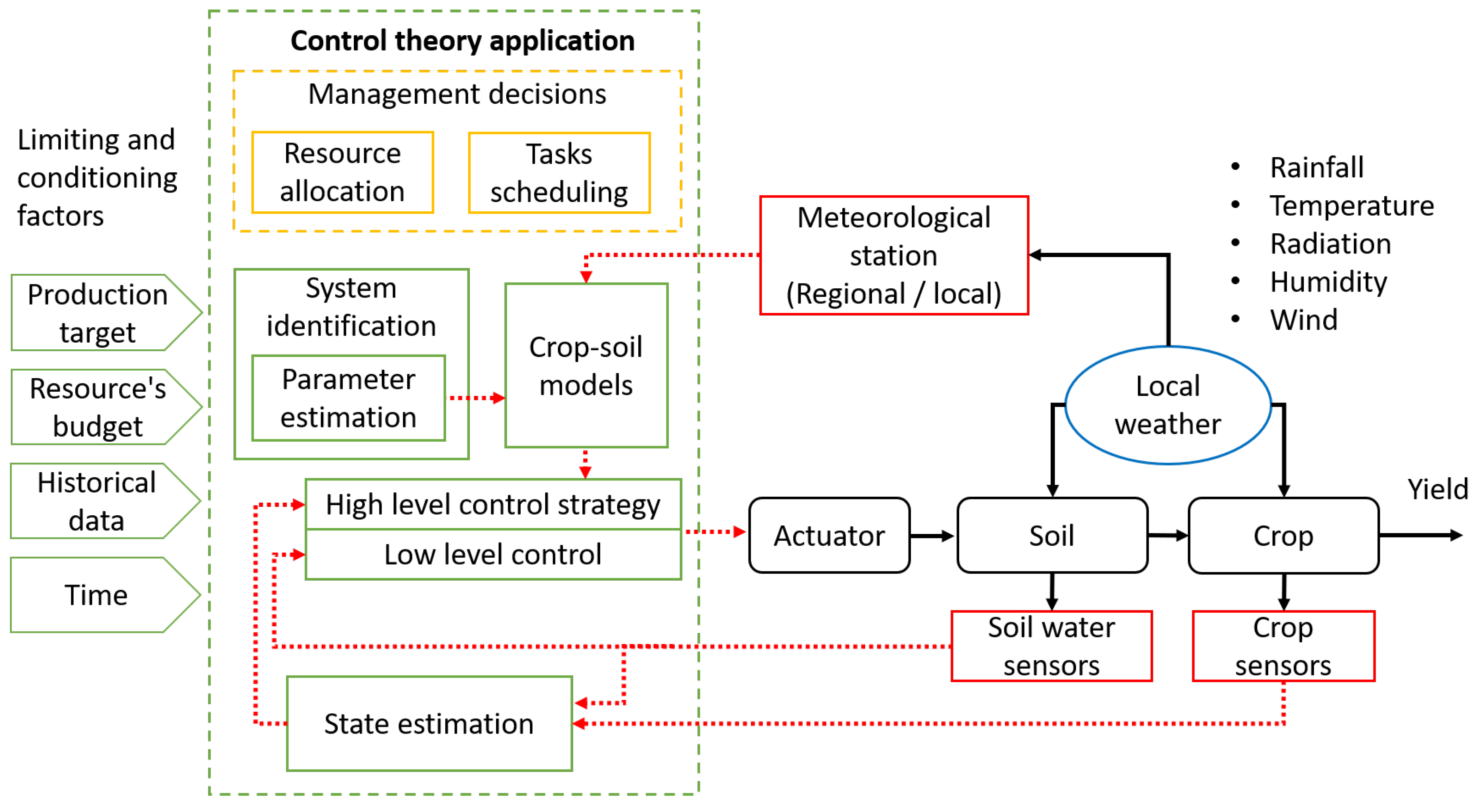
In this present article, the last ten years of developments related to irrigation in agricultural systems are reviewed by following the methodological structure shown in Figure 1. The objective is to highlight the several steps leading to an advanced control strategy, including instrumentation, mathematical modeling, model identification and validation, state estimation (software sensors), and model-based control. The main concepts are illustrated by numerical examples that are carefully worked out. This review builds upon past reviews, such as [16,17], which summarized fundamental control concepts applied to irrigation systems.
The problem of irrigation can be divided into two subproblems, i.e., water transportation and water usage. In this review article, the focus is put on the latter subject, since a complete review about water transportation was recently published [18], where the authors presented a comprehensive description of an open-channel system that included modeling and control features.
This paper is organized as follows. In Section 2, the main components of simulation-oriented models are extracted to propose control-oriented models. Next, Section 3 presents the sensing and measurement elements. Afterwards, in Section 4, the system identification techniques used to determine the model parameters are presented, with an emphasis on parameter uncertainties and model validation. Section 5 reviews state estimation and the reconstruction of non-measured variables. Then, in Section 6, the most popular control techniques are discussed. Section 7 discusses spatial representation and soil heterogeneity. Finally, Section 8 draws conclusions and perspectives.
2. Dynamic Crop–Soil Model Components
Crop-growth models are developed to understand how environmental and management factors affect food production. In a predictive irrigation policy, these models are a core component, as illustrated in Figure 1. Two types of models can be distinguished: (i) simulation-oriented models (SOMs) and (ii) control-oriented models (COMs). The goal of the models in the first category is to faithfully mimic the system behavior and to understand the phenomena influencing crop growth. These models combine mechanistic descriptions of biophysical phenomena and heuristic laws. In [19], the authors presented an extensive list of crop-growth models (however, more than 50% of these models have become obsolete over time). The models in the second group are usually reduced or simplified versions of the previous models. Only 12 of the most cited SOMs are usually considered to build a control-oriented framework (see Table 1) based on a hierarchy in growth and production factors proposed by [20]. These include growth-defining factors, growth-limiting factors, and growth-reducing factors. The growth-defining factors determine the maximum possible growth and are dependent on crop-specific parameters and weather influences, such as temperature and solar radiation. The growth-limiting factors are due to a shortage or excess of water and nutrients such as nitrogen. The growth-reducing factors are due to, e.g., weeds and pests. Some of the mentioned factors are listed in Table 2 for representative SOMs, whose evolution has been reviewed by [21]. Other related works, such as [22], used a dynamic system approach to represent full agricultural production systems. These agricultural production systems include livestock production, economic and labor modules, environmental impact, and social components, which are outside of the scope of this review.
In this review, we describe the crop dynamics for a homogeneous portion of land by following two approaches.
2.1. Crop and Growth Models
Food production includes perennial and seasonal crops. As mentioned in the introduction, water has a determinant influence on the development of both. For instance, large crops of almonds have been identified as the most significant consumers of freshwater, followed by large-scale seasonal crops of rice, alfalfa, sugarcane, wheat, maize, and plantains [23]. Therefore, efficient irrigation offers a global benefit for long- and short-term crops. However, in short-term crops (e.g., cereals and legumes), the excess or lack of water can be catastrophic, since the crop might be under irrecoverable conditions [24]. Consequently, most COMs are focused on seasonal and short-term crops.
The dynamics of crop processes can be described by a system of differential or difference equations, which represent the plant growth with at least three levels of detail. In the first level, the crop growth is limited solely by weather conditions, primarily solar radiation and air temperature. In the second level, growth is water-limited, i.e., limited by the shortage or excess of water supply, in addition to the constraints imposed by weather conditions. In the third level, growth is also limited by the shortage of nutrients—mainly, but not limited to, nitrogen (N)—during some lapses in the growing season. The shortage of other nutrients, such as phosphorus or potassium, follows the same logic as for nitrogen, imposing more restrictive bounds on the growth function. These levels are explained next.

Table 1.
Main inputs and driving and output variables for selected SOM crop models.
| Model | Inputs | Driving Variable | Output Variables | References | |||||||||
|---|---|---|---|---|---|---|---|---|---|---|---|---|---|
| Environmental | Manipulated | ||||||||||||
| Radiation | Temperatures (max, min) | Rainfall Precipitation | Reference Evapotranspiration | Wind | Humidity | Irrigation Moisture | Fertilization | Other | Yield | Other | |||
| APEX | √ | √ | √ | √ | √ | √ | √ | • Soil preparation | Cumulative | √ | • Carbon and nitrogen transformations | [25] | |
| • Pesticide | temperature | • Costs | |||||||||||
| • Crop rotation | |||||||||||||
| • Tillage | |||||||||||||
| APSIM | √ | √ | √ | √ | √ | √ | • Vapor pressure | Thermal time | √ | • Dry matter | [26] | ||
| accumulation | |||||||||||||
| AquaCrop | √ | √ | √ | √ | • CO2 concentration | Water content | √ | • Irrigation | [27] | ||||
| • Soil fertility level | and fluxes | • Water losses | |||||||||||
| • Weed management | • Soil water | ||||||||||||
| CropSyst | √ | √ | √ | • Soil profile | Thermal time | √ | • Above-ground root biomass accumulation | [28] | |||||
| • Management of scheduled events | accumulation | ||||||||||||
| • Fertilization | |||||||||||||
| • Residue fate | |||||||||||||
| DAISY | √ | √ | √ | √ | √ | √ | √ | √ | • Soil properties | Air temperature | • Water balance | [29] | |
| • Sowing/planting | • Heat balance | ||||||||||||
| • Soil tillage | • Solute balance | ||||||||||||
| • Harvest | • Pesticide fate | ||||||||||||
| DNDC | √ | √ | √ | √ | √ | √ | √ | • Redox potential Eh | Air temperature | √ | • Gas emissions | [30,31] | |
| • Oxygen concentration | • N leaching | ||||||||||||
| • Climate file | • Weather | ||||||||||||
| • Soil profile | • Soil carbon sequestration | ||||||||||||
| • Tillage | |||||||||||||
| DSSAT | √ | √ | √ | √ | √ | √ | √ | • CO2 concentration | Thermal time | √ | • Weather | [32] | |
| • Soil profile | accumulation | • Soil profile | |||||||||||
| • Crop profile | • Fertilization | ||||||||||||
| • Management profile | • Irrigation | ||||||||||||
| EPIC | √ | √ | √ | √ | √ | √ | √ | • Soil profile | Solar | √ | • Productivity | [33] | |
| • Soil erosion | radiation | • Waste management | |||||||||||
| • Pesticide | • Plant competition | ||||||||||||
| • Homogeneous soil assumption | • Pesticide fate | ||||||||||||
| • Crop rotation | • Furrow diking | ||||||||||||
| • Tillage | |||||||||||||
| SALUS | √ | √ | √ | √ | √ | • Tillage | Solar | √ | • Development stages | [34] | |||
| • Residue fate | radiation | • Fertilization | |||||||||||
| • Pesticide | • N leaching | ||||||||||||
| • Soil erosion | • Irrigation | ||||||||||||
| STICS | √ | √ | √ | √ | √ | √ | √ | √ | Cropping | Plant carbon | √ | • Nitrate leaching | [35] |
| schema | accumulation [36] | • Drainage | |||||||||||
| SWAP | √ | √ | √ | √ | √ | √ | • Crop rotation | Thermal time | • Dry weight (stems/leaves) | [37] | |||
| • Solute transport | • Water management | ||||||||||||
| WOFOST | √ | √ | √ | √ | √ | √ | √ | √ | • CO2 concentration | Thermal time | √ | • Biomass | [38] |
| • Vapor pressure | • Water use | ||||||||||||
| • Management profile | |||||||||||||
Table 2.
Main functions related to the simulation processes of selected SOMs.
| Model | Water Balance | Nutrient Balance | Evapotranspiration | Growth-Core Main State Variable | Biomass or Yield Formation | Stresses |
|---|---|---|---|---|---|---|
| APEX | Probabilistic distribution |
|
| Potential increase in biomass Monteith 1977 |
| |
| APSIM |
| Nitrogen uptake rate |
|
| Potential biomass accumulation |
|
| AquaCrop | Soil water balance | Salt balance by transfer of solutes |
|
| Cumulative crop transpiration limited by biomass water productivity |
|
| CropSyst |
| N Transformations N absorption rate Chemical budget (salinity, pesticide) |
|
| Tanner and Sinclair (1983), daily biomass accumulation Monteith (1977) at low vapor pressure deficit |
|
| DAISY |
| Nitrogen dynamics |
| • Beer’s law | Accumulation of dry matter and nitrogen |
|
| DNDC | • Algebraic equation |
| Water-use efficiency limited by VPD [39] |
| Daily cumulative temperature conditioned by N demand uptake Water demand uptake | •Water |
| DSSAT | Mass-balance (Differential equations by soil layer) |
|
|
| Growing degree-days (GDD) |
|
| EPIC |
| Leaching equations Sediment transport Mineralization |
|
| Conversion of Intercepted light to biomass |
|
| SALUS | • Mass balance |
| • Penman (1948) (modified by Shuttleworth 2007) |
| Carbon assimilation |
|
| STICS | • Mass balance equation | Functional ratio equation |
|
| Plant carbon accumulation [40] |
|
| SWAP |
| Nitrogen cycle |
| • LAI | Daily net assimilation depending on the intercepted light |
|
| WOFOST | • Mass balance by soil layer | SWAMP model for solute transport | • Penman (1948) |
| Daily net assimilation depending on the intercepted light |
|
2.1.1. First Level
The time evolution of the biomass y is related to the energy provided by sunlight:
where is the growth rate (i.e., the light-use efficiency (g/MJ)), w is the daily intercepted solar radiation (MJ/m), and is the maximum (or potential) biomass, which is related to the crop species and the plant density. After the limit of accumulation of solar energy is reached, the phenology of the crop involves maturity and the natural aging process.
The stresses caused by the lack or excess of environmental inputs, including the shortage of nutrients (which can be remedied by fertilization), are accounted for by models in two ways—first, by speeding up the aging process (e.g., shortening the maturity time or cumulative temperature), and second, by using multiplicative factors of the growth function. These multiplicative stress factors are usually in the range of , where 1 represents a non-stress condition and 0 represents a maximum stress factor. The shape of stress factors is related to the mathematical representation of the observed experimental impact (see Table 3). It is important to note that the multiplicative structure can present serious difficulties for parameter identification.
Other models consider the temperature (T) as a driving variable in order to describe matter formation. The crop grows according to the thermal pace, which corresponds to the number of days that the crop is subject to a range of temperature that has been experimentally proven to be optimal for stomatal exchanges. Crop growth is expressed as the product of the solar radiation (w), the radiation-use efficiency (r), the growth function , and the stress function depending on water (X), temperature (T), and nutrients (N), i.e.,
The growth function is formed by the combination of two logistic shapes: one for the plant vegetative growth from germination to the half of crop life with a positive slope, and the second one for aging from the maturity to harvest with a negative slope.
This type of model can be illustrated by considering the simple case in [43]. Originally, this model was presented in a discrete-time version that used daily steps, as the environmental inputs were typically sensed and reported daily. The potential growth function is given by
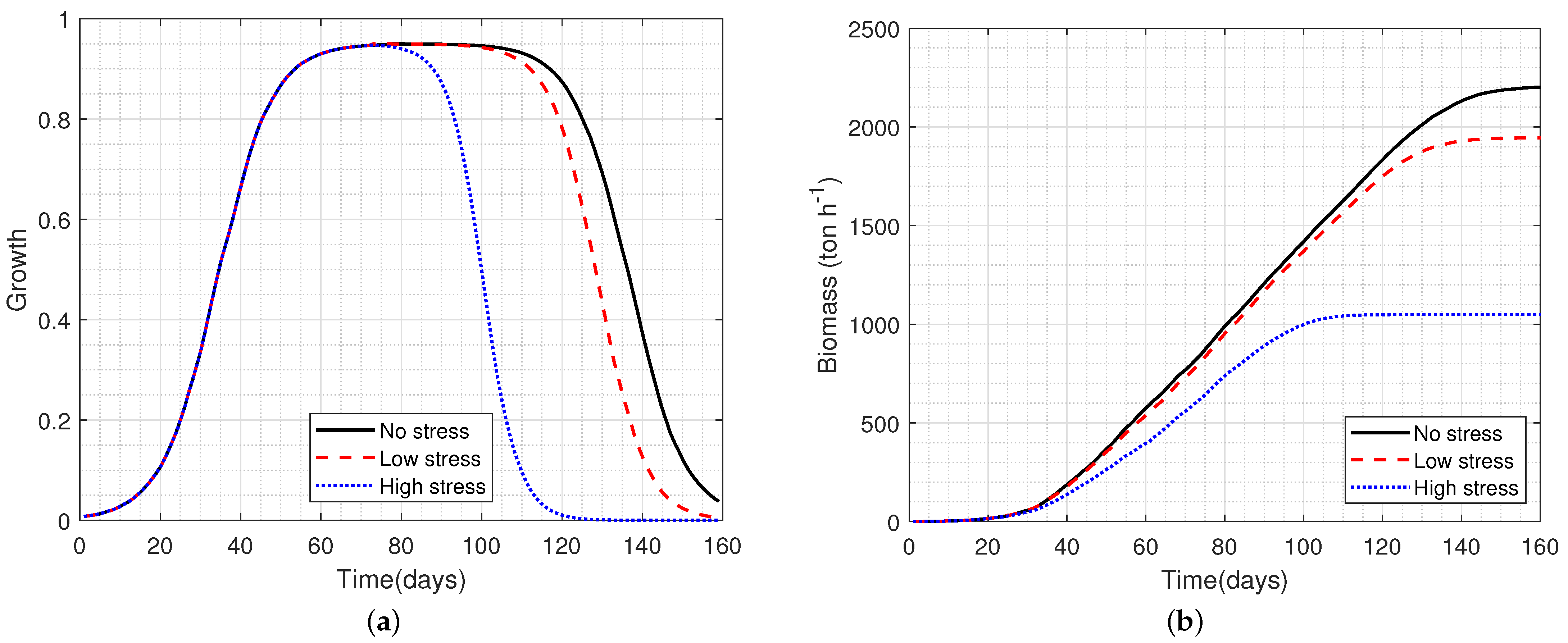
where v represents the cumulative temperature, is the maximum fraction of radiation interception that the crop can reach, is the cumulative temperature requirement for leaf area development to intercept 50% of radiation, is the cumulative temperature requirement from sowing to maturity, and is the temperature aging function accounting for the negative effects of water and temperature stresses. The stress function K, which penalizes the growth in Equation (2), is represented as the product of single environmental stresses, but also includes an additional positive effect of CO (), i.e., .
An example of wheat as a test crop that is sown on a deep loamy soil is shown in Figure 2. Figure 2a shows the shape of the growth function and senescence for non-stress crop growth () and two stress levels (). The early senescence is directly related to stress amplitude. In correspondence, Figure 2b shows the biomass evolution. Notice that any stress factor in Equation (2) affects the growth function by narrowing the bell shape, but also by attenuating its height. Consequently, the presence of stress factors changes the slope of the biomass production graph and its final value.
2.1.2. Second Level
This level of model description involves water supply as a limiting growth factor. Most of the water exchanges occur below the ground, which is why the water-in-soil mass balance equation is considered. This equation is the core of COMs, and is often used to compute the water stress factors. The water content in soil x is computed by
where represents the crop transpiration [47], represents the surface runoff, represents the drainage, u represents the irrigation, and represents the rainfall. As mentioned earlier, a discrete-time version of the model equations is often preferred for practical purposes. This discrete-time version can be obtained using an explicit Euler method for numerical integration, i.e.,
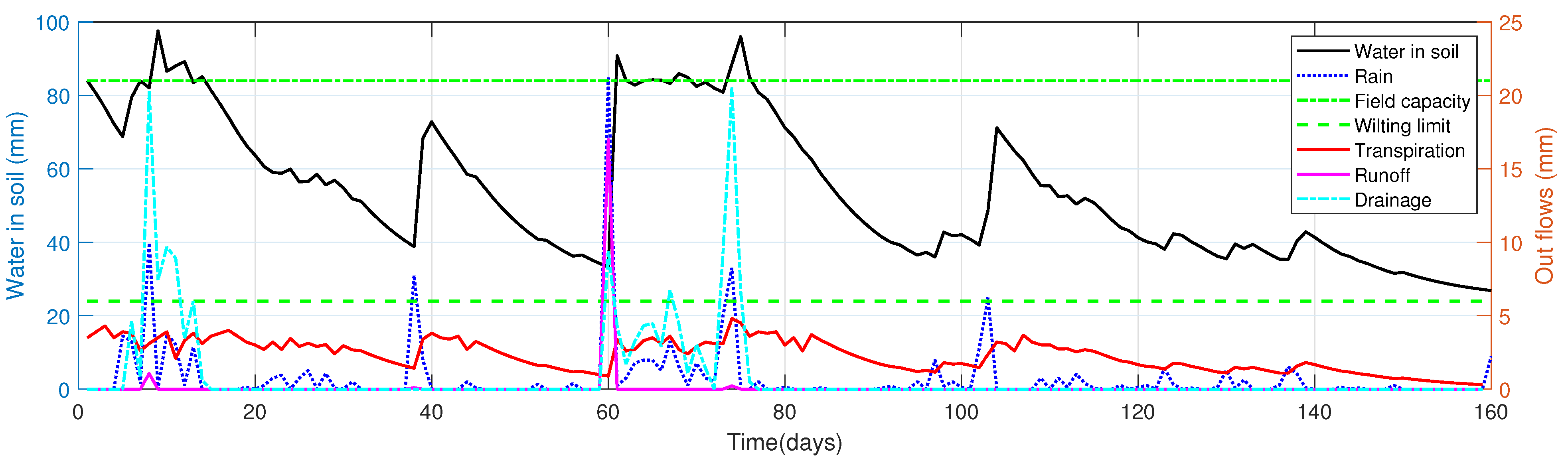
An illustrative example of the behavior of water fluxes in a homogeneous area of soil (Equation (5)) is depicted in Figure 3. The dynamics of water in soil are affected by rainfall and temperature (not in the graph), where the negative effects (i.e., stresses for plants) occur if the water in soil is above the field capacity (saturation) and below the wilting limit. Notice that for proper crop development, it is not necessary to always fill the soil up to the field holding capacity; instead, it is essential to avoid soil dryness.
An example of a more elegant soil representation (i.e., with compartmental vertical layers) is the one proposed by AquaCrop [27]. In this latter model, the differential flow equation is replaced by a set of finite difference equations, which are written in terms of the dependent variable x and the independent variable of time (k). The vertical soil profile is divided into m layers indexed from the surface to the maximum depth considered (), and the time k runs from the sowing to the harvest day. This representation includes the evaporation effect in the surface layer and the rising effect due to the capillarity in the presence of the water table. The moisture content is determined for each layer of the soil and for every time step as follows:
where the superscript i is the index of the soil layer, is the crop transpiration, is the drainage of the soil profile, is the water infiltration into the soil profile (after the subtraction of surface runoff), is the upward movement by capillary rise from a shallow groundwater table, and represents the amount of water lost by soil evaporation. Notice that the advantage of (6) over (5) is the separation of evaporation and transpiration, which address the temperature effect in the top layers, and the vertical movements of water. However, the price to pay is a large number of equations to solve.
2.1.3. Third Level
In this modeling level, the shortage of nitrogen (N) is considered. Nitrogen is fundamental for leaf development, production of chlorophyll, and the synthesis of carbohydrates. However, nitrogen cycles in agriculture are asynchronous and evolve at different rates. There is a slow rate of natural incorporation of nitrogen into the soil by microorganisms and nitrogen uptake by plants, in contrast with the fast rates of nitrogen use inside the plants and the nitrogen compounds withdrawn from the soil. Moreover, nitrogen provided by fertilization is not fully retained in the soil, as only a fraction is used by plants before emission of ammonia into the atmosphere and leaching losses [48].
The nitrogen balance of the soil can be represented as the difference between the nitrogen added by fertilization or mineralization and the nitrogen removed by crop uptake and losses [49]. Therefore, the rate of nitrogen in the soil () is given by:
where is the nitrogen supply through mineralization and biological N fixation, is the fertilizer nitrogen application rate, is the fertilizer nitrogen recovery fraction, and is the rate of nitrogen uptake by the crop, which is calculated as the minimum of the N supply from the soil and the N demand from the crop, and represents the nitrogen losses by leaching.
The net rate of change of nitrogen is
where is the nitrogen translocation and is the loss due to death of the biomass.
A crop is assumed to experience N stress at N concentrations below a critical value for unrestricted growth. To quantify crop response to nitrogen shortage, a Nitrogen Nutrition Index () is defined, ranging from 0 (maximum N shortage) to 1 (no N shortage) as follows:
where , , and are the actual, critical, and residual nitrogen content, respectively. This index, as described in Section 2.1, can affect the growth function as a multiplicative factor or as a modulator of the aging function.
2.2. Compartmental Approach
A modeling approach that differs from the three levels of detail described in the previous subsections is the use of the concepts of storage compartments or pools. In these pools, the organic matter is divided into shoots, or aboveground biomass (AGB), and roots [50]. This compartmental approach has the advantage of discriminating phenological development before germination and after germination, which is convenient for the use of remote sensing technology to measure state variables. As the supply of carbon (C) creates a demand for nitrogen (N), the biomass above and below the ground can be divided into nitrogen and carbon pools. In this case, the biomass (Y in kg m) can be decomposed into the shoot () and root structures (), which are related to the C and N substrate pools in shoots ( and in kgC m) and roots ( and in kgN m). Shoot and root substrate concentrations are defined by
and the differential equations of the state variables are:
where is the net photosynthetic rate (KgC m d), and , are the shoot and root growth rates, and are the substrate fluxes (kg kg), is the flux of C from shoot to root, is the flux of N from root to shoot (Kg m d), , , , and are the output fluxes of C and N from root and shoot to the total product (Kg m d), and are the litter fluxes by the shoot and root structure senescence, and is the growth rate of the total product (kg m d).
This approach based on pools is attractive from a mathematical point of view. However, it poses a challenge for the continuous measurement of the related variables in the pools, particularly the measurement of nitrogen with nondestructive methods, which is still an open research subject.
2.3. State-Space Representation and Variable Definition
To design irrigation strategies, mathematical models can be built based on mass balance equations and mechanistic descriptions of crop–soil subprocesses, as illustrated in Table 2 for some popular SOMs. These models can be cast into a standard nonlinear state-space representation:
where x is the vector of state variables, is the vector of functions that describe the dynamics of the crop–soil system, u represents the vector of inputs, including the environmental inputs and the artificial, or manipulated, inputs , is the set of model parameters, y is the vector of measurement outputs, and is a vector of nonlinear functions relating the state variables with the measurable variables. It is important to note that the crop–soil system is a positive system, i.e., the trajectory of the state variables starting from a positive initial condition always remains positive, regardless of the values of the input variables. However, crop–soil models can preserve this fundamental property only if they are properly formulated. The environmental inputs cannot be influenced, but can be sensed at regular time intervals (for instance daily), whereas the manipulated variables, e.g., fertilization or irrigation, allow one to act on the evolution of the soil–crop system. In Table 2, the main modules (in many reported studies, the models are actually not presented as a global system of equations, but more as a set of software modules achieving the computation of the outcome of specific subprocesses) of selected SOMs are presented based on a functional decomposition of the soil–crop subprocesses. Mass balance modules are solutions of differential or difference equations, whereas other modules are sets of algebraic equations or heuristic formulations, e.g., modules for the evapotranspiration subprocess. Pests, diseases, and weeds may further limit crop production at all developmental stages. However, these factors are not considered in detail in this review, which is dedicated to mathematical modeling and control to support irrigation.
The models have uncertainty related to the inputs, the structure, and the model parameters. These uncertainties can be formulated as probability distributions and can be accounted for in the models. In [51], the authors demonstrated that the uncertainty in the model structure was larger than in the model parameters. However, as SOMs were developed for scientific understanding as well as decision/policy support, the model uncertainty was limited to the bias in the final output, and there was no tracking of how the uncertainty was propagated in the model. As an alternative, in [52], the authors proposed the use of multi-model ensembles (MMEs) to quantify model structural uncertainty, showing that they rely on parts of models that are based on traditional heuristics. In contrast, the uncertainty in a COM can be analyzed by considering the state-space structure.
3. Sensors and Instrumentation
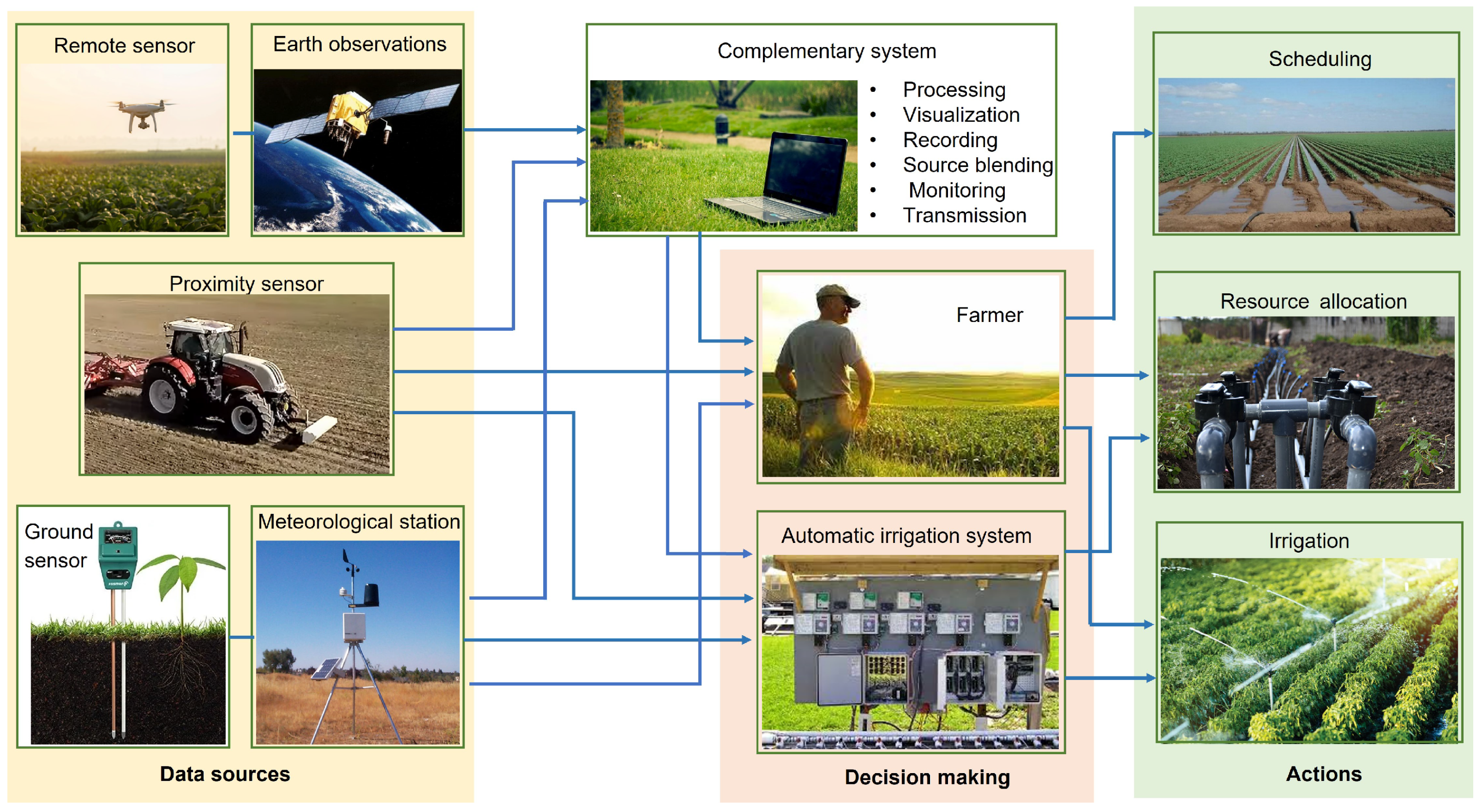
In modern agricultural systems, there is a network of interconnections among farmers, sensors, actuators, machinery, and cultivated areas, forming a so-called cyber–physical–human system (CPHS) [53]. In this context, farmers play a key role as decision makers regarding the management of cultivated areas and food production in general. A global picture is rpresented in Figure 4.
Of course, the information provided by the sensors is a keystone for the development of dynamic models, the estimation of parameters, and the development of more elaborate monitoring and control schemes. For instance, soil moisture (SM) and soil water content (SWC) are essential in irrigation. Traditionally, these variables were measured using probes, e.g., stick probes, neutron probes, phene cells, time-domain reflectometers (TDRs), and tensiometers. The variables are related to physical properties, such as capacitance, resistivity, heat conductance, and mechanical force. Other methods involve collecting samples to be analyzed offline, such as gravimetric measurement, with the drawback of being noncontinuous in time and space. However, more reliable remote methods have gained interest in the last decade due to their coverage of large fields. These include ground-penetrating radar (GPR), aerial photography, multi- and hyperspectral imagery, and electromagnetic induction (EMI). A list of common state variables included in SOMs, as well as the possible types of sensing techniques, is provided in Table 4.
The output equation of the state-space representation (Equation (11b)) is described by the nonlinear vector function , whose structure will highly depend on the underlying physical principles and technology of the measurements. In some specific cases, this nonlinear equation can reduce to a linear one in the form
where is a constant matrix depending on parameter . As a practical example, let us consider the soil moisture sensor presented in [81]. In this work, the output variable y (relative soil moisture) is given by
where w is defined as the ratio of the mass of moisture present in the soil sample to the dried mass of the sample, is the dry unit weight of the soil, and is the unit weight of water. However, many of the output variables are not linearly related to the state variables.
The data acquisition system includes sensors, measurement instruments, transducers, and algorithms. The sensing devices can retrieve information about physical variables through direct (i.e., ground sensors) or indirect contact (i.e., proximity or remote sensing). Traditionally, direct measurements are restricted by the locations of the sensors. This issue was discussed in [82,83], where the main conclusion was that direct measurements are still required as a part of a monitoring and sensing system. Moreover, there are soil properties that can only be sensed directly, e.g., soil organic carbon [84]. The big advantage of ground sensors is the precision and reliability of measurements independently of environmental conditions. The drawback is the limited capability of representing the heterogeneity of a cropping area, as the ground sensors are fixed in particular locations. To alleviate this latter issue, proximity sensors are used for their flexibility. These sensors require one to be close to the crop and soil, but are portable and, therefore, can be installed in unmanned aerial vehicles (UAV), ground robots, or agricultural machinery. However, portability and mobility cannot ensure a simultaneous and global measurement of a cultivated area, and arrays of sensors—especially wireless sensor networks, as suggested by [85,86]—can resolve this global picture. However, this approach is, in turn, limited by the size of the cropping field. Hence, remote sensing (RS) appears as the ultimate solution due to the ability to simultaneously encompass multiple measurements over diverse scales of cropping land. These techniques are particularly well suited for water-related variables in climate change scenarios [87].
RS is a current research and development trend due to its advantages of capturing large amounts of data all at once. RS gathers Earth observations (EOs), which are limited by the orbit and periodicity of satellites, and aerial imagery, which is limited by the frequency of capture and weather conditions. In either case, some variables must be inferred by combining data from multiple sensors in different wavelengths or other variables [67]. For instance, in [61], the evapotranspiration (ET) was derived from the solution of the energy balance equation by using short-wave and long-wave band inputs from satellite sensors to estimate net radiation (), soil heat flux (G), and sensible heat flux (H), with the latent heat flux () obtained as a residual . The LE could then be extrapolated from a quasi-instantaneous value at the time of the satellite overpass to a daily ET value using different methods, such as the evaporative fraction or the reference ET fraction. For large-scale crops, EOs are suited to collecting information that is simultaneously related to crop and field variables. However, the spatial resolution is an issue for non-flat land. A descriptive presentation of the sensors embedded in active satellites is provided in [12], which includes frequency range and spatial and temporal resolution. Optical and thermal sensors are highly sensitive to climatic conditions. For this reason, other sensors, such as synthetic aperture radar (SAR), prove to be an effective technique for monitoring crops and other agricultural targets, as they do not depend on weather conditions [88]. This technology was discussed in [71], which provided a review of the diverse vegetation indexes associated with state variables and discussed the limitations linked to the current information retrieved from SAR sensors and optical/thermal signals to derive variables such as crop height (which is typically sensed by airborne instruments, such as light detection and ranging (LiDAR)).
Reviews of particular data acquisition systems have recently been published. For instance, the authors of [89] surveyed soil moisture measurements by considering ground, proximal, and satellite remote sensing. One of the main challenges is to combine point observations, which are commonly obtained with in situ techniques, such as simple gravimetric sampling or various electromagnetic sensors, with a spatial representation of the water distribution. The problem is to properly capture spatial variability without deploying too many sensors. A possible solution is to combine ground-based and airborne or spaceborne remote sensing techniques to provide a characterization and monitoring of large-scale near-surface soil properties and processes at reasonable temporal and spatial resolutions.
Other environmental and weather variables can be retrieved from either portable or official meteorological stations with regional coverage near the field. The portable stations located in the field have the advantage of reducing the uncertainty of some variables, as their measurement precision is comparable to that of regional meteorological stations, which are usually situated several kilometers away from the field [90].
4. Model Identification
Once a model structure has been established based on mass and energy balances and the use of physical and heuristic relations, the model needs to be calibrated in order to fit to the experimental observations. This operation of model calibration is called parameter estimation or identification in the systems and control literature. System identification gathers a set of statistical techniques that allow the designer to assess the values of model parameters based on signals and data from measurable inputs and outputs. Identification is a broad subject that is well documented in the literature, and we refer the interested reader to a few monographs and textbooks, including [91,92].
Basically, system identification proceeds in several steps, which can be iterated and can be summarized as follows:
- data collection;
- definition of the model objectives (simulation or control) and of the model structure;
- identifiability study;
- parameter estimation;
- evaluation of parameter uncertainties and of confidence intervals in the model prediction;
- model validation and cross-validation.
This section discusses the parameter estimation problem of a crop–soil mathematical model with a known structure, i.e., once the selection of an appropriate model structure has been achieved by following the ideas in Section 2, starting with the question of parameter identifiability.
4.1. Identifiability
Initially, an identifiability study will indicate whether it is possible to determine the parameter values from the available data. More precisely, two types of identifiability studies can be achieved, i.e., structural and practical [93]. The first assesses the possibility of estimating the model parameters given ideal measurements, i.e., it allows the determination of which output signals should be measured, assuming that they are available in continuous time and without noise. Several mathematical approaches can be used to achieve this analysis, and specialized software is available, e.g., DAISY [94], GENSSI [95], SIAN [96], and STRIKE-GOLDD [97], among others. To the best of our knowledge, these methods and software have rarely been used in the modeling of agricultural systems.
Practical identifiability deals with the possibility of assessing all or some of the model parameters under realistic conditions, e.g., sampled data and measurement noise.
The basic tool in this latter study is parametric sensitivity analysis, which can be local [91] or global, and it takes account of the interactions between parameter effects [98,99,100]. Sensitivity analysis has been applied in several studies of crop models. For instance, in [101], the sensitivity of four yield outputs of the APSIM-Sugar model to 13 parameters in rain-fed and irrigated conditions was studied using a global sensitivity method based on the decomposition of variance of the outputs known as Gaussian process emulation. As some crop models are difficult to analyze, as they are not fully mechanistic, but include empirical rules, it might also be interesting to using automatic differentiation tools to achieve sensitivity analysis, as demonstrated in [102].
In this paper, we limit ourselves to a brief introduction of the basic concepts related to a local analysis and consider the model , which is based on the vector of parameters , of the measured output :
In the case of a Gaussian distribution of zero-mean white noise , the Fisher Information Matrix (FIM) can be defined as
where is the covariance matrix of the measurement errors , represents the first-order parametric sensitivity matrix, and M represents the number of data points. The inverse of the FIM provides a lower bound (the so-called Cramer–Rao bound) of the covariance matrix of the parameter estimation errors, i.e.,
A parameter estimation method that can achieve the Cramer–Rao lower bound is called efficient. The FIM is a covariance matrix and, as such, is positive semidefinite. The FIM can be used to assess practical identifiability through a rank condition (a rank-deficient FIM indicates that the model is not identifiable with the data at hand). In turn, if the parameters are identifiable, the Cramer–Rao bound can be used to provide confidence intervals for the estimated parameters (which are, unfortunately, often not given in the published literature on parameter identification of crop models). In general, the use of (local or global) sensitivity analysis will be an important tool for determining the most influential parameters of a model, which requires estimation based on experimental data and may be re-estimated at a later stage if the environmental conditions have changed.
A challenge in the identification of crop–soil models is to deal with a large number of parameters. For instance, DSSAT [32] has more than 300 parameters, STICS [103] has 232 parameters, AquaCrop [104] has 29 parameters, and EPIC [33] has 22 parameters. An approach to reducing the number of parameters to consider is to use specific crop models instead of generic models, e.g., CERES-Wheat [47]. Another option is to derive more compact models, which are usually called summary crop models [6]. These summary models can be developed in several ways—first, as a simplification of full-scale models, e.g., FIELD presented by [105] as a crop–soil subsystem based on APSIM [44] and mini-STICS, a compact and limited version of STICS [103] presented in [106]. Further, compact models can be included in additional software tools, e.g., the OptimiSTICS package [107]. In this case, the aim is to guide the user into parameter estimation under various assumptions. For instance, this software package was used in [108] to estimate a set of parameters of the STICS model. Alternatively, it is possible to build simple new generic crop models on a mechanistic basis, e.g., the simple model [43], which includes 14 equations with 13 parameters. In conclusion, the modeler will generally have to either reduce the model under consideration or to decide on a subset of parameters to estimate in order to ensure practical parameter identifiability before embarking on the actual parameter estimation task.
4.2. Parameter Estimation
Parameter estimation is based on the minimization of the deviation between the model prediction , which depends on a set of parameters , and the measured outputs . A general approach is the maximum likelihood estimator (MLE) [91]:
where M is the number of data points and is the covariance matrix of the measurement errors. Other weighting matrices can be considered, leading to weighted least-squares estimators.
For instance, the generalized least squares (GLS) method was used in [109] to estimate the parameters and to compute the variance–covariance matrix of the cultivar parameters of APSIM [44] and DSSAT [32]. In [108], a Bayesian approach was used to identify the parameter of the STICS crop model [103] based on the Differential Evolution Adaptive Metropolis (DREAM) algorithm [110], which is a variation of the Monte Carlo Markov Chain (MCMC) algorithm.
One of the main dangers in achieving parameter estimation is the risk of local minima of the cost function, leading to biased parameter estimates. This problem can be alleviated by using multistart strategies [111], i.e., repeated optimization starting from a large set of initial parameter guesses sampled in the design space, and through the use of global optimization algorithms [112].
4.3. Model Validation and Uncertainty Analysis
After the model parameters have been determined, model cross-validation should be achieved by comparing the model prediction to a fresh, unseen dataset in order to ensure that the model identification has not been subjected to local minima. The uncertainty of parameters should then be evaluated [113] by using various methodologies, including the Fisher Information Matrix and Monte Carlo analysis.
In [101], an uncertainty propagation analysis was performed assuming both normal and uniform distributions to conclude with a cross-validation. The results confirm the distinct variation of parameter influence between climatic and management conditions. The generalized likelihood uncertainty estimation (GLUE) method was used in [114] to generate 10,000 random parameter sets, including one calibrated parameter set, to explore the effects of parameter uncertainty on model output. GLUE was also exploited in [115] to analyze the DSSAT-CERES model [116]. In [108], the posterior distributions of nine specific crop parameters of the STICS model were sampled with the aim of assessing the growth of a winter wheat culture.
In addition, cross-validation is helpful in dealing with the parameter overfitting problem [117]. In [118], the authors identified ten parameters of AquaCrop and used the MCMC to infer the uncertainty in the parameters by approximating the posterior distribution function with eight experimental datasets.
4.4. Illustrative Example: Water Balance in Soil
To illustrate the previous concepts, the model introduced in Equation (5) is used as an example. This COM is based on water mass balance in soil. Considering that measurements are available for transpiration (), runoff (), drainage (), and available water in the root zone (), the model can be expanded as follows:
where is rainfall, is the reference grass evapotranspiration, and there is no irrigation, i.e., . The set of parameters are the water uptake coefficient , the drainage coefficient , the runoff curve number , the available water capacity , the root zone depth , and the wilting point . is the potential maximum retention depending on the soil type.
First, we conduct an uncertainty and sensitivity analysis by applying Monte Carlo simulations and a Sobol global sensitivity method, as implemented in the Python library UncertainPy [119] and the Sensitivity Analysis Library SALib [120]. In [121], the same model (Equation (18)) was used to compute a drought index named ARID. The authors proposed different probability density functions (PDFs) (i.e., uniform, normal, triangular, and custom) for five parameters (i.e., ) and performed a Fourier amplitude sensitivity test to assess the uncertainty and sensitivity. In contrast with this previous work, we include the wilting point and consider the cumulative available water in the root zone as an output variable, since our objective is to determine the positive and negative impacts of water in soil.
The uncertainty decreases from 40 to 24% when changing from uniform to normal distributions. The parameter is the most relevant, with participation in the global sensitivity. and follow with and , respectively. The full sensitivity test ranks the influence of the parameters as , with negligible influence of the last three. This result suggests that the parameters related to the mechanical properties of soil are more relevant than the ones related to volume constraints.
Next, we perform a parameter estimation based on nonlinear least squares. The basic assumption is that measurements can be collected daily for the four variables (). In the framework of this example, we generate the measurements using the same model and add Gaussian noise to , , , and corresponding to , , , and of the relative standard deviation, respectively. These noise levels are coherent with the corresponding instrumentation [55,122], but they are assumed to be unknown to the process modeler such that a simple weighted least-square approach is used here with a weighting matrix that takes account of the scaling of several variables (the variables have different orders of magnitude, and the scaling avoids distortion in the contributions of the different variables to the cost function). Notice that the information content of the data at hand is crucial. For , only seven measurements contain useful information, and for , sixteen samples do so (see Figure 5b,c). The nominal values of the process emulator parameters and their estimates are presented in Table 5. Confidence intervals of are computed using the Fisher Information Matrix. The model prediction is shown in Figure 5.
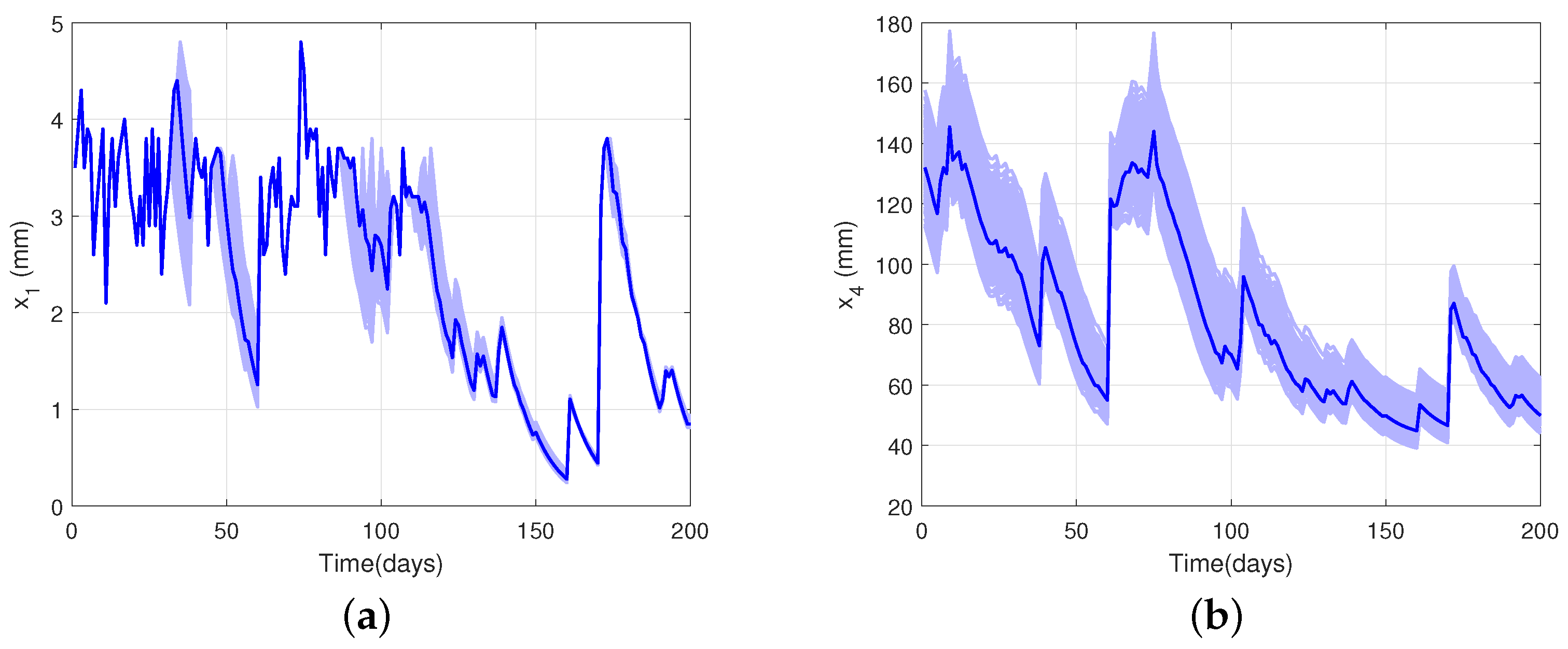
A Monte Carlo simulation is used to assess the uncertainty of the model prediction with the identified parameter values of the parameters in their 95% confidence intervals. The results are shown in Figure 6, where 20,000 runs generate a shaded light-blue region and the solid blue line corresponds to the identified parameters.
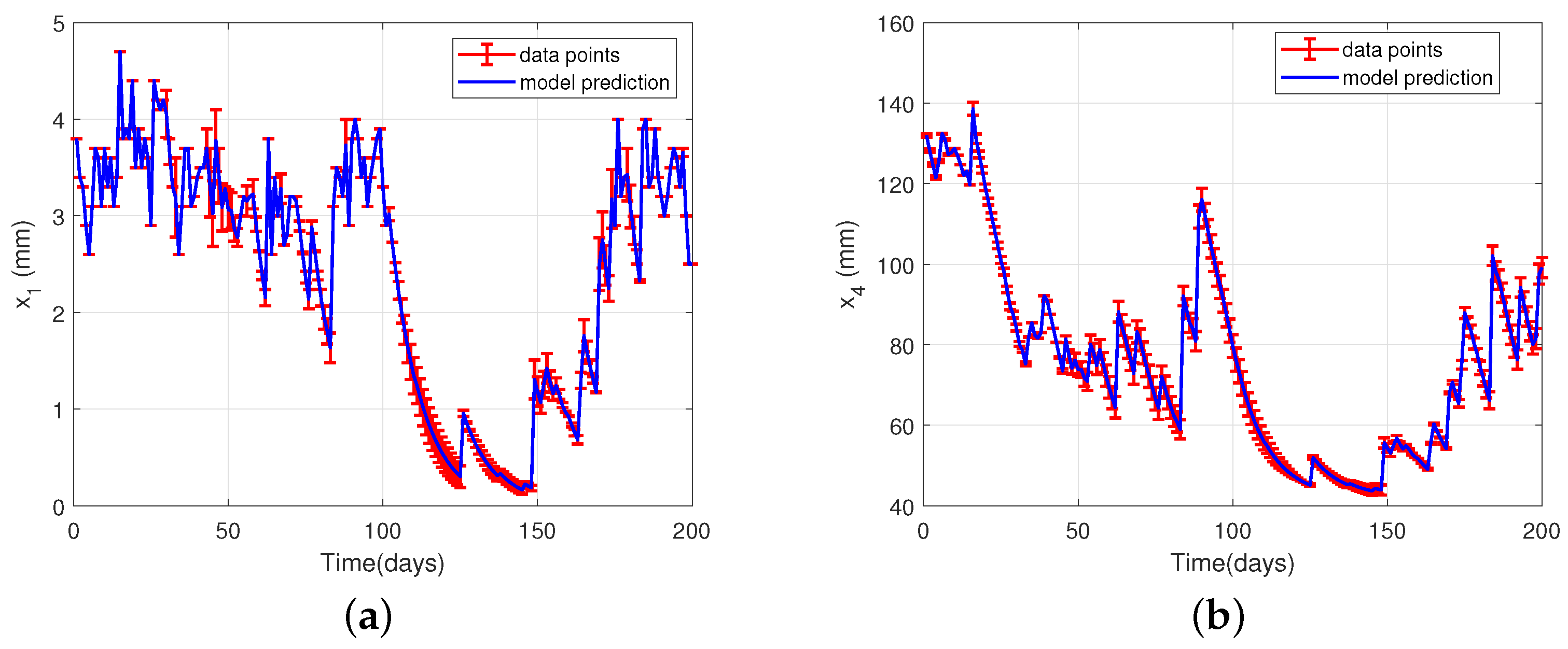
Afterward, cross-validation is performed using a new dataset. The results show that the model with its previously estimated parameters is able to reproduce the dynamic behavior of the soil for other climatic conditions with an error of less than 3%, as shown in Figure 7.
5. State Estimation and Software Sensors
State estimation algorithms allow the reconstruction of non-measured state variables in real time based on a model of the system and some on-line measurements collected from available sensors. In this way, a state estimator constitutes a so-called software sensor, in contrast with a conventional hardware sensor. Aside from the estimation of non-measured state variables, state estimators can also be used for the reconstruction of discrete-time information in continuous time, the fusion of redundant information, the detection and isolation of hardware sensor faults, or the estimation of model parameters. Some introductory surveys related to biological systems can be found in [124,125], and a monograph dedicated to crop systems is found in [113].
In the literature, the notion of data assimilation is also sometimes used to designate the process of combining a mathematical model with measurements to improve the prediction of some state variables or to estimate the initial condition of the model. Historically, data assimilation originates from the field of weather forecasting, and it shares many common features with state estimation techniques, even though the problem of reconstructing non-measured variables and the notion of observability are more typical of the literature dedicated to state estimation. In this review, we will stick with the wording of the system and control community and use state estimation instead of data assimilation.
A state estimator (also known as a state observer) usually has the following extended Luenberger form:
which embeds a copy of the dynamic system for predicting the state trajectory and includes a correction term that measures the deviation between the hardware sensor information y and its prior estimate .
Many state estimation approaches have been proposed. Some of them take account of measurement noise (such as Kalman filters or receding-horizon observers), model uncertainties or disturbances (such as high-gain observers or sliding-mode observers), or uncertainties in model parameters and inputs (such as interval observers). In general, a system property called observability must be checked before embarking on the selection and design of an estimator.
5.1. Observability
A system is said to be observable if the current state vector can be estimated using the information from the sensors collected over a finite period of time. Observability is a structural property of a system, but for nonlinear systems, this property also depends on the input signals.
There are several approaches to the observability analysis of nonlinear systems. The basic one is based on the differentiation of the output and the construction of an observability map. For output j of system (11), the following set of derivatives can be computed:
The observability map is given by:
If a partition of the complete observability map is injective with respect to the state variables, then the system is observable. However, the analytical solution of the nonlinear system is often difficult, or even impossible, to find. Local observability can be checked thanks to the inverse mapping theorem (local inverse):
If the Jacobian is nonsingular, an inverse function exists in some neighborhood of , and local observability is proven.
Note that structural identifiability can be studied as observability by considering the parameters as state variables with zero dynamics [126].
A second approach to global observability analysis is provided by the use of a canonical form [127,128]:
where
A system is said globally observable if
Many systems naturally appear in this form, or can be brought into this form by a change of variables.
Finally, an alternative approach to studying global observability that includes unknown inputs (some system inputs can be uncertain or unknown, such as some environmental conditions) is provided in [129], where a dynamic interpretation of state observability is developed.
Observability Analysis of a Plant-Growth Model
To illustrate these observability tests, let us consider a qualitative mathematical model representing the relationship between supplied water and plant growth [130]. This model relates the water in soil with the water inside the plant for its growth and the amount of dry matter . The state-space representation is given by
where it is assumed that the variables and can be measured.
In this model, the water in soil is related to the biomass production.The soil is modeled as a reservoir of water, and the changes are accounted for in (27a). The first term on the RHS represents the water going out by drainage and evaporation, the second term represents the plant water absorption per unit of time, and the last term is the irrigation input. Next, the water dynamics inside the plant are described by (27b), where the first term on the RHS stands for the water absorbed by the plants, the second term represents the water removed by transpiration, and the last term relates the water used to produce biomass. Finally, the change in biomass is accounted for in Equation (27c), where the first term on the RHS represents the growth function, and the last term represents the plant degradation. A complete description of the parameters and variables is given in Table 6.
Observability can be locally assessed using the Jacobian of the observability map, considering a constant input :
We can see that , provided that either the third or fourth line of the Jacobian matrix is independent of the first two lines. This will be the case if and are not simultaneously equal to zero over some periods of time. This makes sense in an intuitive way, since this would correspond to the situation where the sensors would return zero signals (thus providing no useful information on the dynamical system).
5.2. Software Sensors in Agriculture
Bayesian estimation strategies have been particularly popular in the estimation of variables in crop–soil systems. These techniques can be classified as: (i) Kalman filtering, (ii) variational inference, and (iii) sampling algorithms [131]. Kalman filtering, e.g., the Kalman filter (KF) and the extended Kalman filter (EKF), is based on linear or linearized models and the assumption of Gaussian noise. The optimal estimator (or approximate estimator in the case of the EKF) is provided in the form of the mean and is complemented by the covariance of the estimation error, which is useful in assessing confidence intervals. In variational inference, the approximate posterior distribution of the state (given the measurements) can be obtained through the solution of an optimization problem. However, in crop models with nonlinear observation operators and non-Gaussian observations or non-Gaussian uncertainties, the assumption of normality in the posterior might be a poor choice. In these cases, approaches based on sampling, such as the unscented Kalman filter or particle filters, might be preferable. The first will be appropriate for nonlinear models with Gaussian observations, while the second is appropriate for nonlinear systems with non-Gaussian observations at the price of higher computational expenses. An overview of these estimation techniques and their applications to crop–soil models is given in Table 7 and Table 8. The interested reader is also referred to the review papers in [8,11,132].
The linear and extended Kalman filtering techniques often result in difficulties due to the nonlinearity of the models, and particularly the threshold functions that are often part of their expression. Moreover, the formulation of the uncertainty in the model itself due to parameter, structural, and input uncertainty is often difficult [143].
In [137], the authors used an ensemble Kalman filter (EnKF) in combination with the CERES-Wheat crop-growth model with remote sensing data in order to improve the estimation of LAI parameters. However, the authors did not discuss the setup of the filter or the convergence rate. In [140], the authors implemented an EnKF to estimate the root-zone soil moisture (RZSM) in a coupled SVAT–vegetation model. They compared the results with those of four variants of particle filter implementations. The results showed a small difference in the estimation capabilities of the filters, and the discussion was centered on the selection of the tuning parameters.
Sampling-based algorithms and, particularly, the particle filter (PF) or sequential Monte Carlo filter allow the estimation of information from sources that have non-Gaussian errors. In [144], a variant of the PF, which was called a convolution particle filter, was tested on two models, namely, STICS and LNAS, with several datasets.
The estimation of parameters and state variables can be carried out simultaneously. For instance, in [136], three parameters and three state variables (LAI and soil water content of two soil layers) of the mini-STICS model were estimated. Three techniques were used, namely, the EKF, PF, and VF. The improved performance of the VF method when compared to that of the EKF and PF was demonstrated. The variational filter had a low computational complexity, and the convergence speed of the state and parameter estimation could be adjusted independently. However, the tests of the observers were probably not fully conclusive, as the initial estimates did not display errors (and without initial errors, convergence is not challenged).
5.3. Illustrative Example: State Estimation with a Generic Crop Model
As an illustration of a state estimation problem, an EKF is designed for model (27) with the parameter values given in Table 6. For the sake of simplicity, the irrigation input .
Some underlying assumptions are considered:
- The water absorption rate of the plant is less than or equal to the rate of loss of water from the pond, i.e., ;
- The dry matter accumulation rate of the plant is approximately equal to the rate of decrease in the water inside the plant that goes toward photosynthesis, i.e., ;
- The rate of water loss through transpiration is larger than the rate of water loss through evaporation, i.e., ;
- The degradation rate of the plant is larger than the rate of water loss through evaporation, i.e., ;
- The crop is wheat on a short life cycle of 140 days under no stress conditions. Therefore, water and nutrients are readily available and do not limit growth;
- There is neither damage from pests and diseases nor any competition from weeds growing in the field;
- and can be measured by existing technology, i.e., by RS based on images, and the measurements are collected daily.
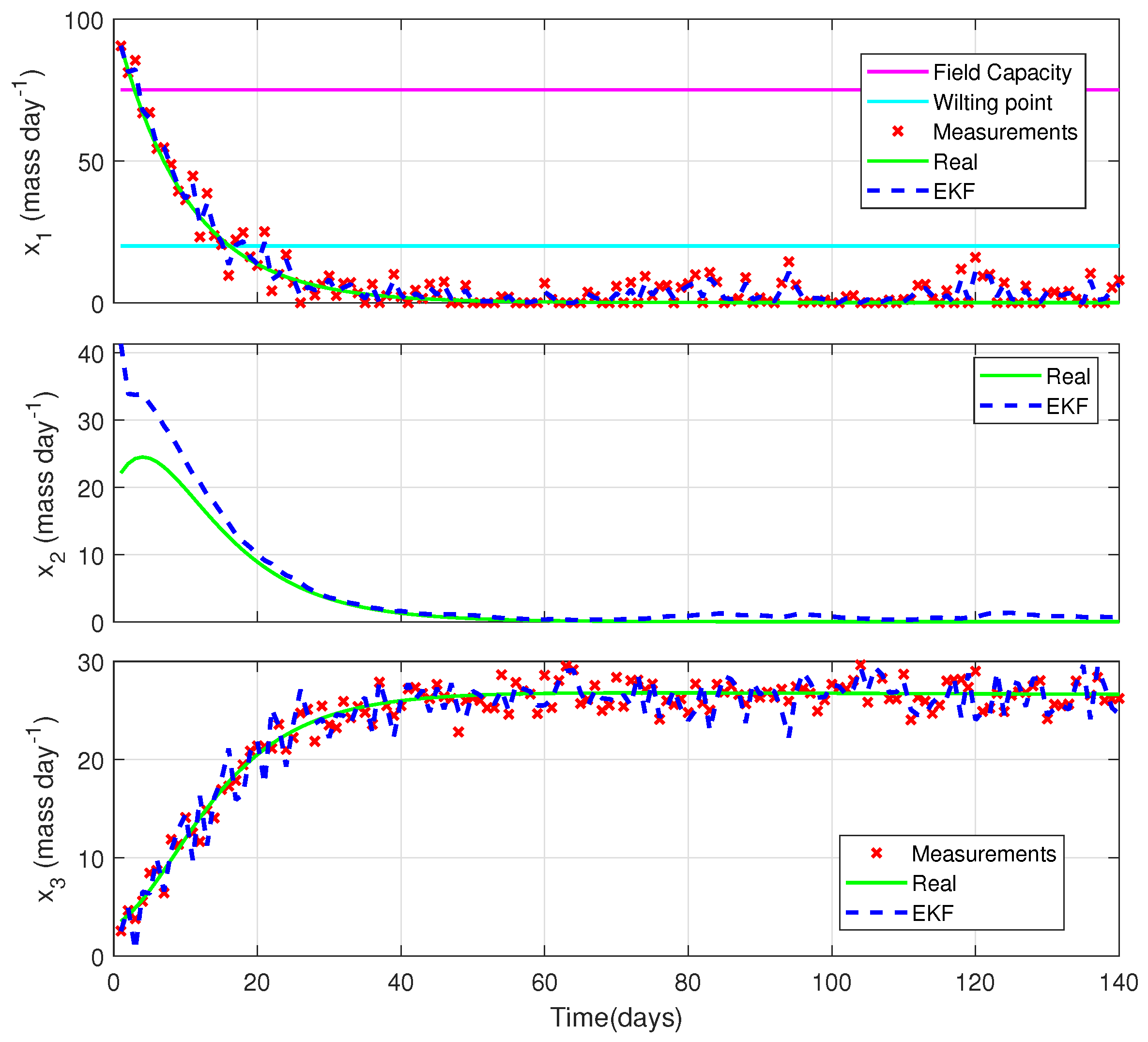
The software sensor is in charge of reconstructing based on the model and the measurements of the other state variables. The EKF design is based on the selection of covariance matrices and , which are based on an evaluation of the model and measurement noises. In Figure 8, the performance of the observer is shown. Notice that the observer uses the first measurement values as initial conditions for the measured variables. On the other hand, the initial value of is intentionally taken far away from the real trajectory to show the convergence speed of the observer (a test that is seldom illustrated in the literature on state estimation in agricultural applications).
6. Irrigation Control
In this section, we review some control techniques that can be used to improve and possibly optimize the irrigation of the field. The manipulated variable is the amount of water supplied in space and time, whereas the output variable is the biomass production. However, in most cases, developers do not consider biomass as an output variable. Instead, they consider a variable related to the soil water content, since models are mostly developed based on the soil behavior.
A preliminary step to the design of an automatic irrigation system is to verify if the state variables can be controlled using the manipulated variables. This issue is accounted for by a property called controllability, which represents the possibility of driving the states of the system from any initial value to a desired final value in a finite time. This property is useful for the control system designer; however, it was not considered in the applications reviewed.
6.1. Control Paradigms
Models for irrigation control can be classified into data-driven and mechanistic models [16]. Data-driven approaches are based on the collection of data from various sensors and the use of machine learning techniques. On the other hand, the mechanistic approach is based on the phenomenological models reviewed in the previous sections, which are possibly simplified to account for only the main phenomena (those that will have a significant effect in a closed-loop operation). Many control techniques can be applied, ranging from classical proportional integral derivative (PID) control to advanced model predictive control (MPC) [17].
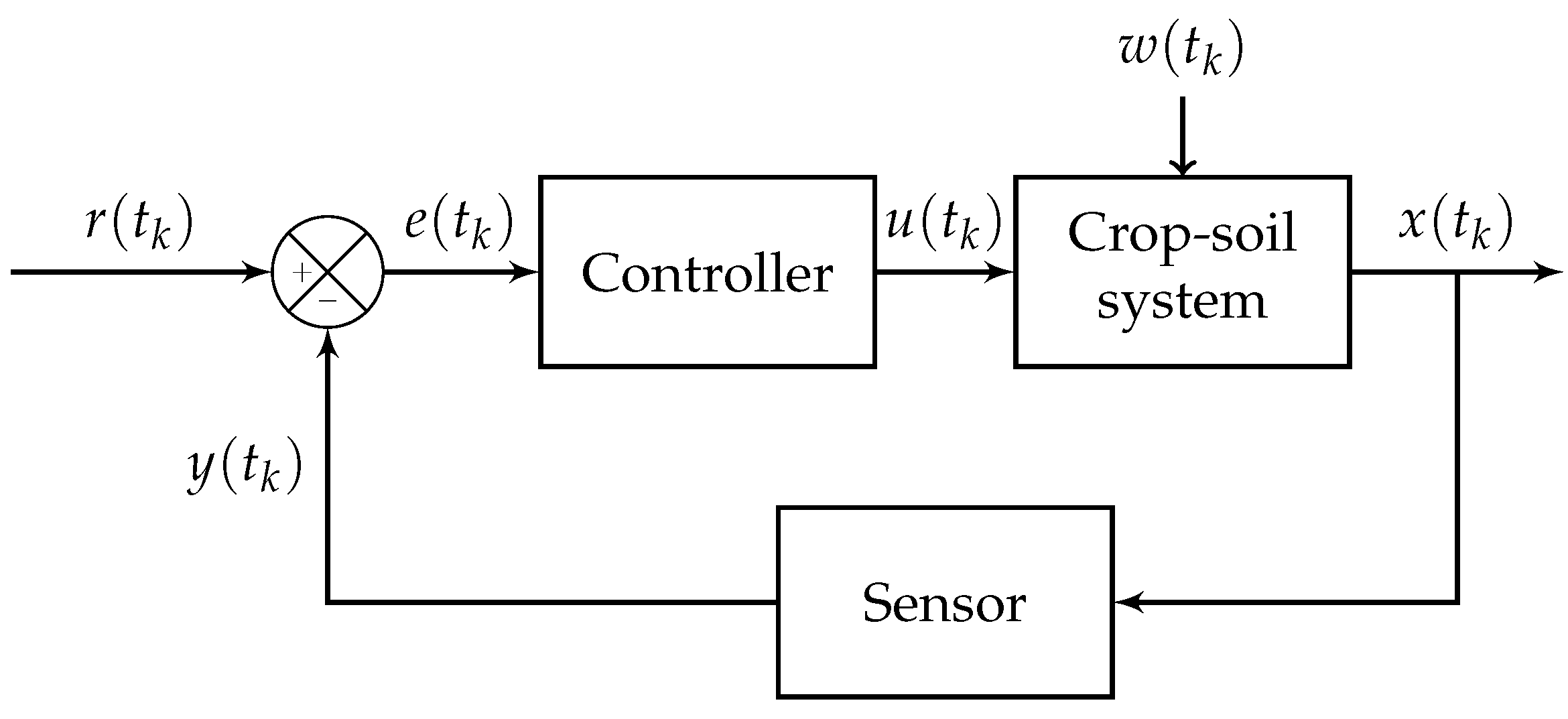
A classical feedback control structure is presented in Figure 9. The error , i.e., the difference between the reference and the measurement signal , feeds the controller, which computes the control action sent to an actuator, e.g., a valve of a sprinkler. A PID controller [145] generates the following control law:
where is the sampling time, is the proportional gain, is the integration time constant, and is the derivative time constant. This control law was implemented and tuned for irrigation using the heuristic methodology in [146], and was further elaborated in [147], where a dielectric tensiometer was used to regulate soil moisture in a strawberry crop.
Model-based control systems make use of a hydrologic model, e.g., related to Equation (4), and some sensors of water in soil. These elements are coupled to an irrigation scheduler to determine the irrigation regime. The main problem is that the output variables (soil moisture, humidity, or evapotranspiration) are related to crop growth, but not to crop performance, which makes irrigation solutions based on the maximization of production suboptimal [148,149]. As an alternative, in [9], the authors described how hydrologic models can be combined with crop-growth models, such as APSIM (i.e., an SOM), to properly account for multiple effects of water on biomass production.
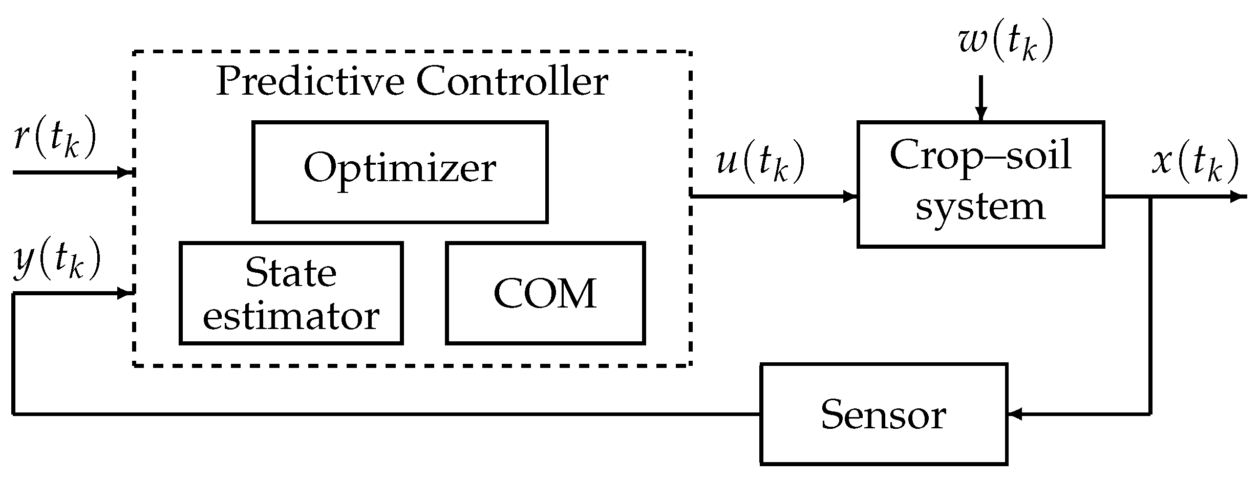
Model predictive control (MPC) is a real-time optimal control strategy based on the numerical optimization of a cost function J (or performance index) over a finite prediction horizon [149]:
where is the ith controlled variable, is the ith reference variable, is the ith manipulated variable move, and and are weighting coefficients, which allow the designer to assign a relative importance to the reference tracking and control energy. is the prediction horizon. The main components of MPC are shown in Figure 10.
In [150], the MPC is formulated based on a linear stochastic state-space model of the soil moisture that incorporates variables such as soil evapotranspiration and deep percolation. A similar work is presented in [148], where the model uses the soil moisture control and the climatic factors to determine the optimal amount of water required by the crop while keeping soil moisture under specific thresholds (avoiding water stress). MPC was also designed based on an SOM, i.e., AquaCrop as a crop emulator, in [151]. In this work, the authors described the design process and discussed the issues related to the implementation. MPC can be improved, as proposed in [152], where the authors presented a data-driven robust model predictive control (DDRMPC) approach for automatic control of irrigation. This control framework integrates a set of mechanistic models, which describe dynamics in soil moisture variations, and data-driven models, which characterize uncertainty in forecast errors of evapotranspiration and precipitation.
Data-driven systems are usually simple and easy to implement. Their main advantage is that they do not require the development of mechanistic models of the crop dynamics [148], and they can be improved over time by optimal learning strategies [153]. In [154], the authors presented an example of a soil moisture control based on continuous measurements of soil water content. This system uses a soil water balance equation to calibrate the model, and then generates an irrigation schedule by combining previous knowledge that is updated by current measurements in an expert system framework. However, the main drawback of these approaches is that they are based on custom solutions for specific areas and crops, which must be constantly calibrated/adapted, and their extrapolation to new situations is not straightforward.
Fuzzy logic has been applied in various agricultural applications, such as irrigation and fertilization. Thanks to its flexibility, this approach allows a qualitative and quantitative interpretation of crop development, which can be defined using expert knowledge and field observations. A design of a fuzzy logic control (FLC) for irrigation was presented in [155]. The stability of the closed-loop system was analyzed using Lyapunov functions. Another application of fuzzy control was presented in [156], where a closed-loop control was integrated with remote sensing. In this work, the objective was to control the speed of the irrigation device (i.e., the central pivot) by sensing the soil moisture, soil temperature, and NDVI.
PID, MPC, and fuzzy logic controllers were compared in [157], where a soil water balance that included soil moisture, temperature, and evapotranspiration was considered. However, the authors only provided general comments on the applicability of such strategies, without design guidelines to support the comparison.
6.2. Illustrative Example: PID and Model Predictive Control
To illustrate an irrigation control application, let us consider the crop–soil model presented in [158]. The discrete-time equations can be summarized as follows:
where the state variables are the water content available in soil , the cumulative temperature , the cumulative temperature until maturity to reach radiation interception due to leaf senescence , and the biomass . The independent inputs are the precipitation , the reference evapotranspiration , the air temperature , solar radiation , and the management input, i.e., the amount of water irrigated u.
The parameters and represent the maximum water content at field capacity, the root water uptake, the maximum daily reduction due to heat stress, the maximum daily reduction due to drought stress, the radiation-use efficiency, and the impact of the growth rate on biomass, respectively. is the drainage coefficient, is the water-holding capacity, is the maximum fraction of radiation interception, and is the cumulative temperature requirement for leaf area development. represents an algebraic function computed by following the procedure described in [113].
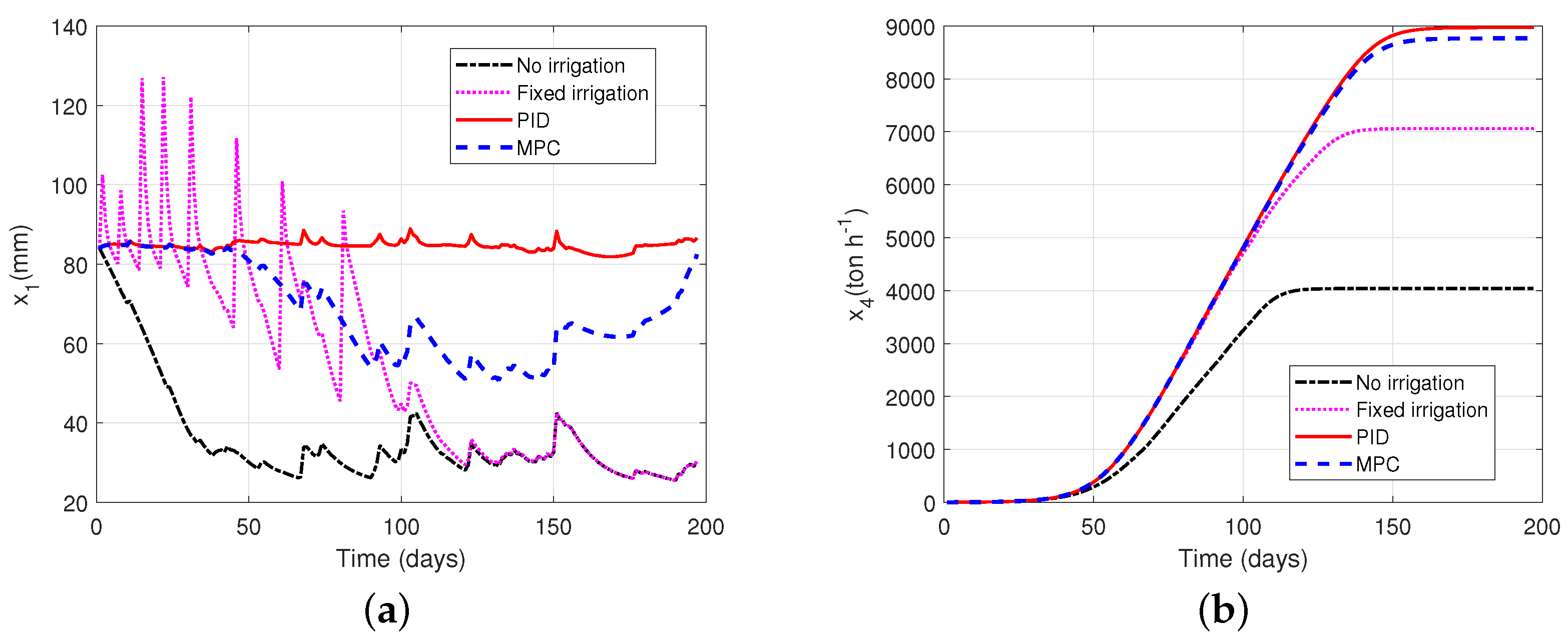
For a wheat crop in loamy soil, a comparison of four situations aimed at assessing the biomass production is presented. First, the model is used under no irrigation policy to establish a minimum performance that is only bounded by environmental conditions. Second, the system is tested while following a fixed irrigation policy, which is a common practice in agriculture. Third, the model is used in a control loop, as shown in Figure 9, using a PID controller, and finally, the model is used in an MPC strategy. The design of the PID controller is achieved with the auto-tune algorithm in Matlab, whereas the MPC cost function targets a maximization of the final biomass in combination with the minimization of the amount of water required to achieve it, i.e.,
where is the prediction horizon in days, is the harvest time, is a weighting factor between the biomass profitability and water expense, and is the maximum amount of water available for the entire crop season. Notice that the proposed cost function considers the maximization of biomass over a limited period , whereas the minimization of the water usage is considered over the full crop season. The reason for the short span of maximization is that biomass production is highly affected by rainfall, while the availability of water for irrigation during the crop season is defined in advance. In addition, the weighting factor gives the designer the possibility to limit the water usage based on the price or availability of the resource.
The results of the comparison are shown in Figure 11 for the water in soil and biomass . Without irrigation, the amount of water in the soil reaches a minimum, and biomass production reaches the lowest level for the season. For the case of fixed irrigation, a total of 340 mm of water is applied in the full season. This irrigation policy increases the production by with respect to the no-irrigation case. However, when control actions are enforced, biomass production and water consumption increase compared to the fixed irrigation scenario. When PID control is active, the reference is to keep the water in the soil at field capacity, implying 405 mm of water, which is about more water than the fixed irrigation. Nevertheless, this represents an increase in biomass production of concerning the case of no irrigation. When the MPC is applied, the increase in the production is about with respect to the no-irrigation case by using about more water than in the case of the fixed irrigation policy. Hence, PID increases production by more than MPC, but requires more water. MPC can be adjusted to relax the constraint related to the water used to reach the same performance as that of the PID control regarding biomass production. The main advantage of MPC is the predictive capability, which can be combined with weather forecasts to reduce water usage to achieve production objectives.
7. Spatial Heterogeneity
The structure of cultivated fields across the world shows non-uniform characteristics. This can be attributed to the topography and soil properties that change spatially and over time. For a continuous modeling of specific soil properties (related to state variables), the formalism of partial differential equations (PDEs) provides an appropriate mathematical representation. In general, the variation of soil properties is considered only with respect to depth, and solvers of the corresponding PDEs have been developed (e.g., for seepage [159]). As an illustration of the above, let us consider the vertical water movement presented in [160], where the soil moisture is computed using the Richards equation, which is a nonlinear parabolic PDE that describes the movement of water in an unsaturated zone. The one-dimensional form of the Richards equation is given by:
where is the volumetric soil moisture, t is time, z is the vertical coordinate (positive in the upward direction), k is the hydraulic conductivity, and h is the pressure head. A discrete-time formulation is used with regard to the standard availability of samples (i.e., daily) and the implementation of the models in dynamic simulation algorithms. Moreover, spatial discretization of the soil into layers or compartments is applied to the vertical water movement, yielding fully discrete (in time and space) simulators. In Section 2, we presented an example of such a model using soil layers, i.e., AquaCrop. A general assumption is a flat land topography with no significant side movements of water.
An alternative to the PDE formalism and the associated spatial discretization is the agent-based approach proposed in [161]. In this work, the layers were treated as agents that interacted with their upper and lower neighbors, exchanging water downward through infiltration or gravity and upward through evaporation or capillarity. The monitoring of vertical water modeling is linked to the availability of sensors, especially for direct measurements. This has limited the applicability of the models.
Partial differential equations have apparently not yet been used by the crop modeling community to represent movements of water to the side, which is probably due to the multidimensional nature of the problem, the more advanced discretization into finite elements or volumes, and the distributed instrumentation required in order to develop monitoring or control.
Instead, other approaches are emerging, such as the stochastic distribution approach [162] and agent-based modeling [123]. In [162], the authors discussed modeling and monitoring complex systems that vary in both space and time given a limited number of agents or sensors providing measurements that are spread out across a large area. They described the land using Gaussian process modeling and addressed data incorporation with a machine learning technique named Kernel Observers. In [123], the idea was to represent the changes across the surface thanks to a discretization of the land into small patches that were linked by the side exchange of water due to the saturation of its retention capacity and the runoff. This latter representation is well suited for crops located in mountain slopes or rugged terrains.
8. Conclusions and Perspectives
A vast body of knowledge about dynamic modeling of crop–soil systems exists, which has resulted in various mathematical models and numerical simulators that allow the understanding and prediction of biomass production as a function of environmental factors and human actions, such as fertilization and irrigation. This modeling approach can be complemented by various concepts of system and control theory to develop efficient monitoring, control, and optimization tools. In this review article, we attempted to draw an overview of these concepts, including model parameter identification, validation, uncertainty analysis, observability analysis, nonlinear state estimation, model-based control, expert systems, and real-time optimization.
Moreover, predictive models can nowadays exploit various sources of information provided by ground sensors, aerial measurements, and satellite imaging, resulting in a big-data perspective and the incorporation of machine learning techniques into the so-called smart farming trend. An important aspect to consider is stochasticity in environmental inputs, which is not a widespread practice in current studies.
There are many appealing directions for future research, including the design of state estimation techniques that exploit sensor networks and take account of uncertainty in the model description and environmental inputs, the development of agent-based models describing soil heterogeneity and incorporating distributed instrumentation and actuation in a possibly asynchronous way, and the design of distributed model predictive control to take full advantage of agent cooperation, real-time optimization, and embedded system technology.
Author Contributions
Conceptualization, N.Q. and A.V.W.; Methodology, N.Q. and A.V.W.; Investigation, J.L.-J., N.Q., and A.V.W.; Formal analysis, J.L.-J.; Software, J.L.-J.; Validation, J.L.-J., Funding acquisition, N.Q. and A.V.W.; Project administration, N.Q. and A.V.W.; Supervision, N.Q. and A.V.W.; Writing—original draft, J.L.-J.; Writing—review and editing, N.Q. and A.V.W. All authors have read and agreed to the published version of the manuscript.
Funding
This research received no external funding.
Data Availability Statement
The data presented in this study are available on request from the corresponding author.
Acknowledgments
The first author acknowledge the support by COLCIENCIAS grant 727.
Conflicts of Interest
The authors declare no conflict of interest.
References
- Campanhola, C.; Pandey, S. Sustainable Food and Agriculture: An Integrated Approach; Academic Press: Cambridge, MA, USA, 2018. [Google Scholar]
- Velasco-Muñoz, J.F.; Aznar-Sánchez, J.A.; Belmonte-Ureña, L.J.; Román-Sánchez, I.M. Sustainable water use in agriculture: A review of worldwide research. Sustainability 2018, 10, 1084. [Google Scholar] [CrossRef] [Green Version]
- Lamnabhi-Lagarrigue, F.; Annaswamy, A.; Engell, S.; Isaksson, A.; Khargonekar, P.; Murray, R.M.; Nijmeijer, H.; Samad, T.; Tilbury, D.; Van den Hof, P. Systems & Control for the future of humanity, research agenda: Current and future roles, impact and grand challenges. Annu. Rev. Control 2017, 43, 1–64. [Google Scholar]
- Nouri, H.; Stokvis, B.; Galindo, A.; Blatchford, M.; Hoekstra, A.Y. Water scarcity alleviation through water footprint reduction in agriculture: The effect of soil mulching and drip irrigation. Sci. Total Environ. 2019, 653, 241–252. [Google Scholar] [CrossRef] [PubMed]
- Ashofteh, P.S.; Bozorg-Haddad, O.; Loáiciga, H.A. Development of adaptive strategies for irrigation water demand management under climate change. J. Irrig. Drain. Eng. 2017, 143, 04016077. [Google Scholar] [CrossRef]
- Jones, J.W.; Antle, J.M.; Basso, B.; Boote, K.J.; Conant, R.T.; Foster, I.; Godfray, H.C.J.; Herrero, M.; Howitt, R.E.; Janssen, S.; et al. Toward a new generation of agricultural system data, models, and knowledge products: State of agricultural systems science. Agric. Syst. 2017, 155, 269–288. [Google Scholar] [CrossRef]
- Jones, J.W.; Antle, J.M.; Basso, B.; Boote, K.J.; Conant, R.T.; Foster, I.; Godfray, H.C.J.; Herrero, M.; Howitt, R.E.; Janssen, S.; et al. Brief history of agricultural systems modeling. Agric. Syst. 2017, 155, 240–254. [Google Scholar] [CrossRef] [PubMed]
- Jin, X.; Kumar, L.; Li, Z.; Feng, H.; Xu, X.; Yang, G.; Wang, J. A review of data assimilation of remote sensing and crop models. Eur. J. Agron. 2018, 92, 141–152. [Google Scholar] [CrossRef]
- Siad, S.M.; Iacobellis, V.; Zdruli, P.; Gioia, A.; Stavi, I.; Hoogenboom, G. A review of coupled hydrologic and crop growth models. Agric. Water Manag. 2019, 224, 105746. [Google Scholar] [CrossRef]
- Zhou, H.; Zhao, W. Modeling soil water balance and irrigation strategies in a flood-irrigated wheat-maize rotation system. A case in dry climate, China. Agric. Water Manag. 2019, 221, 286–302. [Google Scholar] [CrossRef]
- Huang, J.; Gómez-Dans, J.L.; Huang, H.; Ma, H.; Wu, Q.; Lewis, P.E.; Liang, S.; Chen, Z.; Xue, J.H.; Wu, Y.; et al. Assimilation of remote sensing into crop growth models: Current status and perspectives. Agric. For. Meteorol. 2019, 276–277, 107609. [Google Scholar] [CrossRef]
- Karthikeyan, L.; Chawla, I.; Mishra, A.K. A review of remote sensing applications in agriculture for food security: Crop growth and yield, irrigation, and crop losses. J. Hydrol. 2020, 586, 124905. [Google Scholar] [CrossRef]
- Liakos, K.G.; Busato, P.; Moshou, D.; Pearson, S.; Bochtis, D. Machine learning in agriculture: A review. Sensors 2018, 18, 2674. [Google Scholar] [CrossRef] [PubMed] [Green Version]
- Lytos, A.; Lagkas, T.; Sarigiannidis, P.; Zervakis, M.; Livanos, G. Towards smart farming: Systems, frameworks and exploitation of multiple sources. Comput. Netw. 2020, 172, 107147. [Google Scholar] [CrossRef]
- Cobbenhagen, A.; Antunes, D.; van de Molengraft, M.; Heemels, W. Opportunities for control engineering in arable precision agriculture. Annu. Rev. Control. 2021, 51, 47–55. [Google Scholar] [CrossRef]
- Romero, R.; Muriel, J.; García, I.; de la Peña, D.M. Research on automatic irrigation control: State of the art and recent results. Agric. Water Manag. 2012, 114, 59–66. [Google Scholar] [CrossRef]
- McCarthy, A.C.; Hancock, N.H.; Raine, S.R. Advanced process control of irrigation: The current state and an analysis to aid future development. Irrig. Sci. 2013, 31, 183–192. [Google Scholar] [CrossRef]
- Conde, G.; Quijano, N.; Ocampo-Martinez, C. Modeling and control in open-channel irrigation systems: A review. Annu. Rev. Control. 2021, 51, 163–171. [Google Scholar] [CrossRef]
- Di Paola, A.; Valentini, R.; Santini, M. An overview of available crop growth and yield models for studies and assessments in agriculture. J. Sci. Food Agric. 2016, 96, 709–714. [Google Scholar] [CrossRef]
- Rossiter, D. Biophysical models in land evaluation. In Encyclopedia of Land Use, Land cCover and Soil Sciences: Land Evaluation; EOLSS Publishers/UNESCO: Oxford, UK, 2009; Volume 2, pp. 181–195. [Google Scholar]
- Keating, B.A.; Thorburn, P.J. Modelling crops and cropping systems—Evolving purpose, practice and prospects. Eur. J. Agron. 2018, 100, 163–176. [Google Scholar] [CrossRef]
- Walters, J.P.; Archer, D.W.; Sassenrath, G.F.; Hendrickson, J.R.; Hanson, J.D.; Halloran, J.M.; Vadas, P.; Alarcon, V.J. Exploring agricultural production systems and their fundamental components with system dynamics modelling. Ecol. Model. 2016, 333, 51–65. [Google Scholar] [CrossRef] [Green Version]
- Bruinsma, J. World Agriculture: Towards 2015/2030: An FAO Perspective; Routledge: London, UK, 2017. [Google Scholar]
- Yu, L.; Gao, X.; Zhao, X. Global synthesis of the impact of droughts on crops’ water-use efficiency (WUE): Towards both high WUE and productivity. Agric. Syst. 2020, 177, 102723. [Google Scholar] [CrossRef]
- Williams, J.R.; Izaurralde, R.; Singh, V.; Frevert, D. The APEX model. In Watershed Models; CRC Press: Boca Raton, FL, USA, 2006; pp. 437–482. [Google Scholar]
- Keating, B.A.; Carberry, P.S.; Hammer, G.L.; Probert, M.E.; Robertson, M.J.; Holzworth, D.; Huth, N.I.; Hargreaves, J.N.; Meinke, H.; Hochman, Z.; et al. An overview of APSIM, a model designed for farming systems simulation. Eur. J. Agron. 2003, 18, 267–288. [Google Scholar] [CrossRef] [Green Version]
- Steduto, P.; Hsiao, T.C.; Raes, D.; Fereres, E. AquaCrop—The FAO Crop Model to Simulate Yield Response to Water: I. Concepts and Underlying Principles. Agron. J. 2009, 101, 426–437. [Google Scholar] [CrossRef] [Green Version]
- Stöckle, C.O.; Donatelli, M.; Nelson, R. CropSyst, a cropping systems simulation model. Eur. J. Agron. 2003, 18, 289–307. [Google Scholar] [CrossRef]
- Abrahamsen, P.; Hansen, S. Daisy: An open soil-crop-atmosphere system model. Environ. Model. Softw. 2000, 15, 313–330. [Google Scholar] [CrossRef]
- Li, C.; Frolking, S.; Crocker, G.J.; Grace, P.R.; Klír, J.; Körchens, M.; Poulton, P.R. Simulating trends in soil organic carbon in long-term experiments using the DNDC model. Geoderma 1997, 81, 45–60. [Google Scholar] [CrossRef]
- Gilhespy, S.L.; Anthony, S.; Cardenas, L.; Chadwick, D.; del Prado, A.; Li, C.; Misselbrook, T.; Rees, R.M.; Salas, W.; Sanz-Cobena, A.; et al. First 20 years of DNDC (DeNitrification DeComposition): Model evolution. Ecol. Model. 2014, 292, 51–62. [Google Scholar] [CrossRef] [Green Version]
- Jones, J.W.; Hoogenboom, G.; Porter, C.H.; Boote, K.J.; Batchelor, W.D.; Hunt, L.; Wilkens, P.W.; Singh, U.; Gijsman, A.J.; Ritchie, J.T. The DSSAT cropping system model. Eur. J. Agron. 2003, 18, 235–265. [Google Scholar] [CrossRef]
- Williams, J.; Jones, C.; Kiniry, J.; Spanel, D.A. The EPIC crop growth model. Trans. ASAE 1989, 32, 497–0511. [Google Scholar] [CrossRef]
- Basso, B.; Ritchie, J.T. Simulating Crop Growth and Biogeochemical Fluxes in Response to Land Management Using the SALUS Model; Oxford University Press: Oxford, UK, 2015; Volume 2015. [Google Scholar]
- Brisson, N.; Mary, B.; Ripoche, D.; Jeuffroy, M.H.; Ruget, F.; Nicoullaud, B.; Gate, P.; Devienne-Barret, F.; Antonioletti, R.; Durr, C.; et al. STICS: A generic model for the simulation of crops and their water and nitrogen balances. I. Theory and parameterization applied to wheat and corn. Agronomie 1998, 18, 311–346. [Google Scholar] [CrossRef]
- de Wit, C.T. Transpiration and Crop Yields; Technical Report; Wageningen University: Wageningen, The Netherlands, 1958. [Google Scholar]
- Kroes, J.; Van Dam, J.; Bartholomeus, R.; Groenendijk, P.; Heinen, M.; Hendriks, R.; Mulder, H.; Supit, I.; Van Walsum, P. SWAP Version 4; Technical Report; Wageningen Environmental Research: Wageningen, The Netherlands, 2017. [Google Scholar]
- Van Diepen, C.v.; Wolf, J.; Van Keulen, H.; Rappoldt, C. WOFOST: A simulation model of crop production. Soil Use Manag. 1989, 5, 16–24. [Google Scholar] [CrossRef]
- Aber, J.D.; Federer, C.A. A generalized, lumped-parameter model of photosynthesis, evapotranspiration and net primary production in temperate and boreal forest ecosystems. Oecologia 1992, 92, 463–474. [Google Scholar] [CrossRef] [PubMed]
- De Wit, C. Potential Photosynthesis Crop Surfaces. Neth. J. Agric. Sci. 1959, 7, 141–149. [Google Scholar]
- Jiang, T.; Dou, Z.; Liu, J.; Gao, Y.; Malone, R.W.; Chen, S.; Feng, H.; Yu, Q.; Xue, G.; He, J. Simulating the Influences of Soil Water Stress on Leaf Expansion and Senescence of Winter Wheat. Agric. For. Meteorol. 2020, 291, 108061. [Google Scholar] [CrossRef]
- Woli, P.; Jones, J.W.; Ingram, K.T.; Fraisse, C.W. Agricultural Reference Index for Drought (ARID). Agron. J. 2012, 104, 287–300. [Google Scholar] [CrossRef]
- Zhao, C.; Liu, B.; Xiao, L.; Hoogenboom, G.; Boote, K.J.; Kassie, B.T.; Pavan, W.; Shelia, V.; Kim, K.S.; Hernandez-Ochoa, I.M.; et al. A SIMPLE crop model. Eur. J. Agron. 2019, 104, 97–106. [Google Scholar] [CrossRef]
- Holzworth, D.P.; Huth, N.I.; deVoil, P.G.; Zurcher, E.J.; Herrmann, N.I.; McLean, G.; Chenu, K.; van Oosterom, E.J.; Snow, V.; Murphy, C.; et al. APSIM—Evolution towards a new generation of agricultural systems simulation. Environ. Model. Softw. 2014, 62, 327–350. [Google Scholar] [CrossRef]
- Wang, E.; Martre, P.; Zhao, Z.; Ewert, F.; Maiorano, A.; Rötter, R.P.; Kimball, B.A.; Ottman, M.J.; Wall, G.W.; White, J.W.; et al. The uncertainty of crop yield projections is reduced by improved temperature response functions. Nat. Plants 2017, 3, 17102. [Google Scholar] [CrossRef] [Green Version]
- Donatelli, M.; Magarey, R.D.; Bregaglio, S.; Willocquet, L.; Whish, J.P.; Savary, S. Modelling the impacts of pests and diseases on agricultural systems. Agric. Syst. 2017, 155, 213–224. [Google Scholar] [CrossRef]
- Ritchie, J. A user-orientated model of the soil water balance in wheat. In Wheat Growth and Modelling; Springer: Berlin/Heidelberg, Germany, 1985; pp. 293–305. [Google Scholar]
- Cameron, K.; Di, H.J.; Moir, J. Nitrogen losses from the soil/plant system: A review. Ann. Appl. Biol. 2013, 162, 145–173. [Google Scholar] [CrossRef]
- Shibu, M.; Leffelaar, P.; Van Keulen, H.; Aggarwal, P. LINTUL3, a simulation model for nitrogen-limited situations: Application to rice. Eur. J. Agron. 2010, 32, 255–271. [Google Scholar] [CrossRef]
- Thornley, J.H.; France, J. Mathematical Models in Agriculture: Quantitative Methods for the Plant, Animal and Ecological Sciences; Cabi: Wallingford, UK, 2007. [Google Scholar]
- Zhang, S.; Tao, F.; Zhang, Z. Uncertainty from model structure is larger than that from model parameters in simulating rice phenology in China. Eur. J. Agron. 2017, 87, 30–39. [Google Scholar] [CrossRef] [Green Version]
- Wallach, D.; Thorburn, P.J. Estimating uncertainty in crop model predictions: Current situation and future prospects. Eur. J. Agron. 2017, 88, A1–A7. [Google Scholar] [CrossRef]
- Sowe, S.K.; Simmon, E.; Zettsu, K.; de Vaulx, F.; Bojanova, I. Cyber-Physical-Human Systems: Putting People in the Loop. IT Prof. 2016, 18, 10–13. [Google Scholar] [CrossRef] [Green Version]
- Mittelbach, H.; Lehner, I.; Seneviratne, S.I. Comparison of four soil moisture sensor types under field conditions in Switzerland. J. Hydrol. 2012, 430, 39–49. [Google Scholar] [CrossRef]
- Kashyap, B.; Kumar, R. Sensing Methodologies in Agriculture for Soil Moisture and Nutrient Monitoring. IEEE Access 2021, 9, 14095–14121. [Google Scholar] [CrossRef]
- Zare, E.; Arshad, M.; Zhao, D.; Nachimuthu, G.; Triantafilis, J. Two-dimensional time-lapse imaging of soil wetting and drying cycle using EM38 data across a flood irrigation cotton field. Agric. Water Manag. 2020, 241, 106383. [Google Scholar] [CrossRef]
- Zare, E.; Wang, J.; Zhao, D.; Arshad, M.; Triantafilis, J. Scope to map available water content using proximal sensed electromagnetic induction and gamma-ray spectrometry data. Agric. Water Manag. 2021, 247, 106705. [Google Scholar] [CrossRef]
- Qu, Y.; Zhu, Y.; Han, W.; Wang, J.; Ma, M. Crop leaf area index observations with a wireless sensor network and its potential for validating remote sensing products. IEEE J. Sel. Top. Appl. Earth Obs. Remote Sens. 2013, 7, 431–444. [Google Scholar] [CrossRef]
- Viña, A.; Gitelson, A.A.; Nguy-Robertson, A.L.; Peng, Y. Comparison of different vegetation indices for the remote assessment of green leaf area index of crops. Remote Sens. Environ. 2011, 115, 3468–3478. [Google Scholar] [CrossRef]
- Li, X.; Liu, Q.; Yang, R.; Zhang, H.; Zhang, J.; Cai, E. The design and implementation of the leaf area index sensor. Sensors 2015, 15, 6250–6269. [Google Scholar] [CrossRef] [PubMed] [Green Version]
- Neale, C.M.U.; Geli, H.M.E.; Kustas, W.P.; Alfieri, J.G.; Gowda, P.H.; Evett, S.R.; Prueger, J.H.; Hipps, L.E.; Dulaney, W.P.; Chávez, J.L.; et al. Soil water content estimation using a remote sensing based hybrid evapotranspiration modeling approach. Adv. Water Resour. 2012, 50, 152–161. [Google Scholar] [CrossRef]
- Dalezios, N.R.; Dercas, N.; Spyropoulos, N.V.; Psomiadis, E. Remotely sensed methodologies for crop water availability and requirements in precision farming of vulnerable agriculture. Water Resour. Manag. 2019, 33, 1499–1519. [Google Scholar] [CrossRef]
- Campos, I.; González-Gómez, L.; Villodre, J.; González-Piqueras, J.; Suyker, A.E.; Calera, A. Remote sensing-based crop biomass with water or light-driven crop growth models in wheat commercial fields. Field Crop. Res. 2018, 216, 175–188. [Google Scholar] [CrossRef]
- Meng, B.; Ge, J.; Liang, T.; Yang, S.; Gao, J.; Feng, Q.; Cui, X.; Huang, X.; Xie, H. Evaluation of remote sensing inversion error for the above-ground biomass of alpine meadow grassland based on multi-source satellite data. Remote Sens. 2017, 9, 372. [Google Scholar] [CrossRef] [Green Version]
- Kumar, L.; Mutanga, O. Remote sensing of above-ground biomass. Remote Sens. 2017, 9, 935. [Google Scholar] [CrossRef] [Green Version]
- Lu, D.; Chen, Q.; Wang, G.; Liu, L.; Li, G.; Moran, E. A survey of remote sensing-based aboveground biomass estimation methods in forest ecosystems. Int. J. Digit. Earth 2016, 9, 63–105. [Google Scholar] [CrossRef]
- Khanal, S.; Fulton, J.; Shearer, S. An overview of current and potential applications of thermal remote sensing in precision agriculture. Comput. Electron. Agric. 2017, 139, 22–32. [Google Scholar] [CrossRef]
- Lu, L.; Kuenzer, C.; Wang, C.; Guo, H.; Li, Q. Evaluation of three MODIS-derived vegetation index time series for dryland vegetation dynamics monitoring. Remote Sens. 2015, 7, 7597–7614. [Google Scholar] [CrossRef] [Green Version]
- Shen, L.; He, Y.; Guo, X. Suitability of the normalized difference vegetation index and the adjusted transformed soil-adjusted vegetation index for spatially characterizing loggerhead shrike habitats in North American mixed prairie. J. Appl. Remote Sens. 2013, 7, 073574. [Google Scholar] [CrossRef]
- Ren, H.; Zhou, G.; Zhang, F. Using negative soil adjustment factor in soil-adjusted vegetation index (SAVI) for aboveground living biomass estimation in arid grasslands. Remote Sens. Environ. 2018, 209, 439–445. [Google Scholar] [CrossRef]
- Chao, Z.; Liu, N.; Zhang, P.; Ying, T.; Song, K. Estimation methods developing with remote sensing information for energy crop biomass: A comparative review. Biomass Bioenergy 2019, 122, 414–425. [Google Scholar] [CrossRef]
- Amaral, L.R.; Molin, J.P.; Portz, G.; Finazzi, F.B.; Cortinove, L. Comparison of crop canopy reflectance sensors used to identify sugarcane biomass and nitrogen status. Precis. Agric. 2015, 16, 15–28. [Google Scholar] [CrossRef]
- Krienke, B.; Ferguson, R.B.; Schlemmer, M.; Holland, K.; Marx, D.; Eskridge, K. Using an unmanned aerial vehicle to evaluate nitrogen variability and height effect with an active crop canopy sensor. Precis. Agric. 2017, 18, 900–915. [Google Scholar] [CrossRef] [Green Version]
- Peng, J.; Loew, A.; Zhang, S.; Wang, J.; Niesel, J. Spatial downscaling of satellite soil moisture data using a vegetation temperature condition index. IEEE Trans. Geosci. Remote Sens. 2015, 54, 558–566. [Google Scholar] [CrossRef]
- Caldwell, T.G.; Bongiovanni, T.; Cosh, M.H.; Halley, C.; Young, M.H. Field and laboratory evaluation of the CS655 soil water content sensor. Vadose Zone J. 2018, 17, 1–16. [Google Scholar] [CrossRef] [Green Version]
- Bittelli, M. Measuring soil water content: A review. HortTechnology 2011, 21, 293–300. [Google Scholar] [CrossRef]
- Zhao, Y.; Tong, R.j.; Chen, M.Q.; Xia, F. Relative humidity sensor based on hollow core fiber filled with GQDs-PVA. Sens. Actuators B Chem. 2019, 284, 96–102. [Google Scholar] [CrossRef]
- Che, Y.; Ma, S.; Xing, F.; Li, S.; Dai, Y. An improvement of the retrieval of temperature and relative humidity profiles from a combination of active and passive remote sensing. Meteorol. Atmos. Phys. 2019, 131, 681–695. [Google Scholar] [CrossRef]
- Yao, X.; Yao, X.; Jia, W.; Tian, Y.; Ni, J.; Cao, W.; Zhu, Y. Comparison and intercalibration of vegetation indices from different sensors for monitoring above-ground plant nitrogen uptake in winter wheat. Sensors 2013, 13, 3109–3130. [Google Scholar] [CrossRef]
- Yang, B.; Wang, M.; Sha, Z.; Wang, B.; Chen, J.; Yao, X.; Cheng, T.; Cao, W.; Zhu, Y. Evaluation of aboveground nitrogen content of winter wheat using digital imagery of unmanned aerial vehicles. Sensors 2019, 19, 4416. [Google Scholar] [CrossRef] [PubMed] [Green Version]
- SU, S.L.; Singh, D.; Baghini, M.S. A critical review of soil moisture measurement. Measurement 2014, 54, 92–105. [Google Scholar] [CrossRef]
- Fritz, S.; See, L.; Bayas, J.C.L.; Waldner, F.; Jacques, D.; Becker-Reshef, I.; Whitcraft, A.; Baruth, B.; Bonifacio, R.; Crutchfield, J.; et al. A comparison of global agricultural monitoring systems and current gaps. Agric. Syst. 2019, 168, 258–272. [Google Scholar] [CrossRef]
- Chauhan, S.; Darvishzadeh, R.; Boschetti, M.; Pepe, M.; Nelson, A. Remote sensing-based crop lodging assessment: Current status and perspectives. ISPRS J. Photogramm. Remote Sens. 2019, 151, 124–140. [Google Scholar] [CrossRef] [Green Version]
- Li, X.; McCarty, G.W. Application of topographic analyses for mapping spatial patterns of soil properties. In Geospatial Analyses of Earth Observation (EO) Data; IntechOpen: London, UK, 2019. [Google Scholar] [CrossRef] [Green Version]
- Sreeja, B.; Manoj Kumar, S.; Sherubha, P.; Sasirekha, S. Crop monitoring using wireless sensor networks. Mater. Today Proc. 2020. [Google Scholar] [CrossRef]
- Thakur, D.; Kumar, Y.; Kumar, A.; Singh, P.K. Applicability of wireless sensor networks in precision agriculture: A review. Wirel. Pers. Commun. 2019, 107, 471–512. [Google Scholar] [CrossRef]
- Cui, X.; Guo, X.; Wang, Y.; Wang, X.; Zhu, W.; Shi, J.; Lin, C.; Gao, X. Application of remote sensing to water environmental processes under a changing climate. J. Hydrol. 2019, 574, 892–902. [Google Scholar] [CrossRef]
- Liu, C.A.; Chen, Z.X.; Yun, S.H.A.O.; Chen, J.S.; Hasi, T.; PAN, H.Z. Research advances of SAR remote sensing for agriculture applications: A review. J. Integr. Agric. 2019, 18, 506–525. [Google Scholar] [CrossRef] [Green Version]
- Babaeian, E.; Sadeghi, M.; Jones, S.B.; Montzka, C.; Vereecken, H.; Tuller, M. Ground, proximal, and satellite remote sensing of soil moisture. Rev. Geophys. 2019, 57, 530–616. [Google Scholar] [CrossRef] [Green Version]
- Tenzin, S.; Siyang, S.; Pobkrut, T.; Kerdcharoen, T. Low cost weather station for climate-smart agriculture. In Proceedings of the 2017 9th international conference on knowledge and smart technology (KST), Chonburi, Thailand, 1–4 February 2017; pp. 172–177. [Google Scholar]
- Walter, E.; Pronzato, L. Identification of Parametric Models from Experimental Data; Springer: Berlin/Heidelberg, Germany, 1997. [Google Scholar]
- Keesman, K.J. System Identification: An Introduction; Springer Science & Business Media: Berlin/Heidelberg, Germany, 2011. [Google Scholar]
- Wieland, F.G.; Hauber, A.L.; Rosenblatt, M.; Tönsing, C.; Timmer, J. On structural and practical identifiability. Curr. Opin. Syst. Biol. 2021, 25, 60–69. [Google Scholar] [CrossRef]
- Bellu, G.; Saccomani, M.P.; Audoly, S.; D’Angiò, L. DAISY: A new software tool to test global identifiability of biological and physiological systems. Comput. Methods Programs Biomed. 2007, 88, 52–61. [Google Scholar] [CrossRef] [Green Version]
- Chis, O.; Banga, J.R.; Balsa-Canto, E. GenSSI: A software toolbox for structural identifiability analysis of biological models. Bioinformatics 2011, 27, 2610–2611. [Google Scholar] [CrossRef] [Green Version]
- Hong, H.; Ovchinnikov, A.; Pogudin, G.; Yap, C. SIAN: Software for structural identifiability analysis of ODE models. Bioinformatics 2019, 35, 2873–2874. [Google Scholar] [CrossRef]
- Villaverde, A.F. Observability and structural identifiability of nonlinear biological systems. Complexity 2019, 2019. [Google Scholar] [CrossRef] [Green Version]
- Monod, H.; Naud, C.; Makowski, D. Uncertainty and sensitivity analysis for crop models. In Working with Dynamic Crop Models: Evaluation, Analysis, Parameterization, and Applications; Elsevier: Amsterdam, The Netherlands, 2006; Volume 4, pp. 55–100. [Google Scholar]
- Lamboni, M.; Makowski, D.; Lehuger, S.; Gabrielle, B.; Monod, H. Multivariate global sensitivity analysis for dynamic crop models. Field Crop. Res. 2009, 113, 312–320. [Google Scholar] [CrossRef]
- Sarrazin, F.; Pianosi, F.; Wagener, T. Global Sensitivity Analysis of environmental models: Convergence and validation. Environ. Model. Softw. 2016, 79, 135–152. [Google Scholar] [CrossRef] [Green Version]
- Gunarathna, M.; Sakai, K.; Nakandakari, T.; Momii, K.; Kumari, M. Sensitivity Analysis of Plant-and Cultivar-Specific Parameters of APSIM-Sugar Model: Variation between Climates and Management Conditions. Agronomy 2019, 9, 242. [Google Scholar] [CrossRef] [Green Version]
- Lauvernet, C.; Hascoet, L.; Le Dimet, F.X.; Baret, F. Using Automatic Differentiation to study the sensitivity of a crop model. In Recent Advances in Algorithmic Differentiation; Springer: Berlin/Heidelberg, Germany, 2012; pp. 59–69. [Google Scholar]
- Brisson, N.; Gary, C.; Justes, E.; Roche, R.; Mary, B.; Ripoche, D.; Zimmer, D.; Sierra, J.; Bertuzzi, P.; Burger, P.; et al. An overview of the crop model STICS. Eur. J. Agron. 2003, 18, 309–332. [Google Scholar] [CrossRef]
- Vanuytrecht, E.; Raes, D.; Steduto, P.; Hsiao, T.C.; Fereres, E.; Heng, L.K.; Vila, M.G.; Moreno, P.M. AquaCrop: FAO’s crop water productivity and yield response model. Environ. Model. Softw. 2014, 62, 351–360. [Google Scholar] [CrossRef]
- Tittonell, P.; Corbeels, M.; Van Wijk, M.T.; Giller, K.E. FIELD—A summary simulation model of the soil–crop system to analyse long-term resource interactions and use efficiencies at farm scale. Eur. J. Agron. 2010, 32, 10–21. [Google Scholar] [CrossRef]
- Tremblay, M.; Wallach, D. Comparison of parameter estimation methods for crop models. Agronomie 2004, 24, 351–365. [Google Scholar] [CrossRef] [Green Version]
- Wallach, D.; Buis, S.; Lecharpentier, P.; Bourges, J.; Clastre, P.; Launay, M.; Bergez, J.E.; Guerif, M.; Soudais, J.; Justes, E. A package of parameter estimation methods and implementation for the STICS crop-soil model. Environ. Model. Softw. 2011, 26, 386–394. [Google Scholar] [CrossRef]
- Dumont, B.; Leemans, V.; Mansouri, M.; Bodson, B.; Destain, J.P.; Destain, M.F. Parameter identification of the STICS crop model, using an accelerated formal MCMC approach. Environ. Model. Softw. 2014, 52, 121–135. [Google Scholar] [CrossRef] [Green Version]
- Wallach, D.; Nissanka, S.P.; Karunaratne, A.S.; Weerakoon, W.; Thorburn, P.J.; Boote, K.J.; Jones, J.W. Accounting for both parameter and model structure uncertainty in crop model predictions of phenology: A case study on rice. Eur. J. Agron. 2017, 88, 53–62. [Google Scholar] [CrossRef]
- Vrugt, J.A.; Ter Braak, C.J. DREAM (D): An adaptive Markov Chain Monte Carlo simulation algorithm to solve discrete, noncontinuous, and combinatorial posterior parameter estimation problems. Hydrol. Earth Syst. Sci. 2011, 15, 3701–3713. [Google Scholar] [CrossRef] [Green Version]
- Martí, R.; Resende, M.G.; Ribeiro, C.C. Multi-start methods for combinatorial optimization. Eur. J. Oper. Res. 2013, 226, 1–8. [Google Scholar] [CrossRef]
- Floudas, C.A.; Gounaris, C.E. A review of recent advances in global optimization. J. Glob. Optim. 2009, 45, 3–38. [Google Scholar] [CrossRef]
- Wallach, D.; Makowski, D.; Jones, J.W.; Brun, F. Working with Dynamic Crop Models: Methods, Tools and Examples for Agriculture and Environment; Academic Press: Cambridge, MA, USA, 2018. [Google Scholar]
- Yan, L.; Jin, J.; Wu, P. Impact of parameter uncertainty and water stress parameterization on wheat growth simulations using CERES-Wheat with GLUE. Agric. Syst. 2020, 181, 102823. [Google Scholar] [CrossRef]
- Li, Z.; He, J.; Xu, X.; Jin, X.; Huang, W.; Clark, B.; Yang, G.; Li, Z. Estimating genetic parameters of DSSAT-CERES model with the GLUE method for winter wheat (Triticum aestivum L.) production. Comput. Electron. Agric. 2018, 154, 213–221. [Google Scholar] [CrossRef] [Green Version]
- Jones, J.W.; He, J.; Boote, K.J.; Wilkens, P.; Porter, C.; Hu, Z. Estimating DSSAT cropping system cultivar-specific parameters using Bayesian techniques. Methods Introd. Syst. Model. Into Agric. Res. 2011, 2, 365–393. [Google Scholar]
- Seidel, S.J.; Palosuo, T.; Thorburn, P.; Wallach, D. Towards improved calibration of crop models—Where are we now and where should we go? Eur. J. Agron. 2018, 94, 25–35. [Google Scholar] [CrossRef]
- Zhang, T.; Su, J.; Liu, C.; Chen, W.H. Bayesian calibration of AquaCrop model for winter wheat by assimilating UAV multi-spectral images. Comput. Electron. Agric. 2019, 167, 105052. [Google Scholar] [CrossRef]
- Tennøe, S.; Halnes, G.; Einevoll, G.T. Uncertainpy: A python toolbox for uncertainty quantification and sensitivity analysis in computational neuroscience. Front. Neuroinform. 2018, 12, 49. [Google Scholar] [CrossRef] [PubMed] [Green Version]
- Herman, J.; Usher, W. SALib: An open-source Python library for sensitivity analysis. J. Open Source Softw. 2017, 2, 97. [Google Scholar] [CrossRef]
- Woli, P.; Jones, J.W.; Ingram, K.T. Assessing the Agricultural Reference Index for Drought (ARID) Using Uncertainty and Sensitivity Analyses. Agron. J. 2013, 105, 150–160. [Google Scholar] [CrossRef]
- Huang, D.; Wang, J.; Khayatnezhad, M. Estimation of actual evapotranspiration using soil moisture balance and remote sensing. Iran. J. Sci. Technol. Trans. Civ. Eng. 2021, 45, 2779–2786. [Google Scholar] [CrossRef]
- Lopez-Jimenez, J.; Quijano, N.; Vande Wouwer, A. An Agent-Based Crop Model Framework for Heterogeneous Soils. Agronomy 2021, 11, 85. [Google Scholar] [CrossRef]
- Bogaerts, P.; Vande Wouwer, A. Software sensors for bioprocesses. ISA Trans. 2003, 42, 547–558. [Google Scholar] [CrossRef]
- Goffaux, G.; Vande Wouwer, A. Bioprocess state estimation: Some classical and less classical approaches. In Control and Observer Design for Nonlinear Finite and Infinite Dimensional Systems; Springer: Berlin/Heidelberg, Germany, 2005; pp. 111–128. [Google Scholar]
- Villaverde, A.F.; Tsiantis, N.; Banga, J.R. Full observability and estimation of unknown inputs, states and parameters of nonlinear biological models. J. R. Soc. Interface 2019, 16, 20190043. [Google Scholar] [CrossRef] [Green Version]
- Zeitz, M. Observability canonical (phase-variable) form for non-linear time-variable systems. Int. J. Syst. Sci. 1984, 15, 949–958. [Google Scholar] [CrossRef]
- Gauthier, J.P.; Kupka, I.A. Observability and observers for nonlinear systems. SIAM J. Control. Optim. 1994, 32, 975–994. [Google Scholar] [CrossRef]
- Moreno, J.A.; Rocha-Cózatl, E.; Wouwer, A.V. A dynamical interpretation of strong observability and detectability concepts for nonlinear systems with unknown inputs: Application to biochemical processes. Bioprocess Biosyst. Eng. 2014, 37, 37–49. [Google Scholar] [CrossRef] [PubMed]
- Díaz-González, V.; Rojas-Palma, A.; Carrasco-Benavides, M. How Does Irrigation Affect Crop Growth? A Mathematical Modeling Approach. Mathematics 2022, 10, 151. [Google Scholar] [CrossRef]
- Bannister, R. A review of operational methods of variational and ensemble-variational data assimilation. Q. J. R. Meteorol. Soc. 2017, 143, 607–633. [Google Scholar] [CrossRef] [Green Version]
- Dorigo, W.A.; Zurita-Milla, R.; de Wit, A.J.; Brazile, J.; Singh, R.; Schaepman, M.E. A review on reflective remote sensing and data assimilation techniques for enhanced agroecosystem modeling. Int. J. Appl. Earth Obs. Geoinf. 2007, 9, 165–193. [Google Scholar] [CrossRef]
- Sedano, F.; Kempeneers, P.; Hurtt, G. A Kalman filter-based method to generate continuous time series of medium-resolution NDVI images. Remote Sens. 2014, 6, 12381–12408. [Google Scholar] [CrossRef] [Green Version]
- Lü, H.; Yu, Z.; Zhu, Y.; Drake, S.; Hao, Z.; Sudicky, E.A. Dual state-parameter estimation of root zone soil moisture by optimal parameter estimation and extended Kalman filter data assimilation. Adv. Water Resour. 2011, 34, 395–406. [Google Scholar] [CrossRef]
- Agyeman, B.T.; Bo, S.; Sahoo, S.R.; Yin, X.; Liu, J.; Shah, S.L. Soil moisture map construction by sequential data assimilation using an extended Kalman filter. J. Hydrol. 2021, 598, 126425. [Google Scholar] [CrossRef]
- Mansouri, M.; Dumont, B.; Destain, M.F. Modeling and prediction of nonlinear environmental system using Bayesian methods. Comput. Electron. Agric. 2013, 92, 16–31. [Google Scholar] [CrossRef] [Green Version]
- Rui, L.; Li, C.j.; Dong, Y.y.; Feng, L.; Wang, J.h.; Yang, X.d.; Pan, Y.c. Assimilation of remote sensing and crop model for LAI estimation based on ensemble Kaiman Filter. Agric. Sci. China 2011, 10, 1595–1602. [Google Scholar]
- Zhao, Y.; Chen, S.; Shen, S. Assimilating remote sensing information with crop model using Ensemble Kalman Filter for improving LAI monitoring and yield estimation. Ecol. Model. 2013, 270, 30–42. [Google Scholar] [CrossRef]
- Huang, J.; Sedano, F.; Huang, Y.; Ma, H.; Li, X.; Liang, S.; Tian, L.; Zhang, X.; Fan, J.; Wu, W. Assimilating a synthetic Kalman filter leaf area index series into the WOFOST model to improve regional winter wheat yield estimation. Agric. For. Meteorol. 2016, 216, 188–202. [Google Scholar] [CrossRef]
- Nagarajan, K.; Judge, J.; Graham, W.D.; Monsivais-Huertero, A. Particle filter-based assimilation algorithms for improved estimation of root-zone soil moisture under dynamic vegetation conditions. Adv. Water Resour. 2011, 34, 433–447. [Google Scholar] [CrossRef]
- Fang, H.; Liang, S.; Hoogenboom, G.; Teasdale, J.; Cavigelli, M. Corn-yield estimation through assimilation of remotely sensed data into the CSM-CERES-Maize model. Int. J. Remote Sens. 2008, 29, 3011–3032. [Google Scholar] [CrossRef]
- Yildirak, K.; Kalaylıoglu, Z.; Mermer, A. Bayesian estimation of crop yield function: Drought based wheat prediction model for tigem farms. Environ. Ecol. Stat. 2015, 22, 693–704. [Google Scholar] [CrossRef]
- Nychka, D.; Anderson, J.L. Data assimilation. In Handbook of Spatial Statistics; CRC Press: Boca Raton, FL, USA, 2010; pp. 477–492. [Google Scholar]
- Chen, Y.; Cournède, P.H. Data assimilation to reduce uncertainty of crop model prediction with convolution particle filtering. Ecol. Model. 2014, 290, 165–177. [Google Scholar] [CrossRef] [Green Version]
- Visioli, A. Practical PID Control; Springer Science & Business Media: Berlin/Heidelberg, Germany, 2006. [Google Scholar]
- Goodchild, M.; Kühn, K.; Jenkins, M.; Burek, K.; Button, A. A method for precision closed-loop irrigation using a modified PID control algorithm. Sens. Transducers 2015, 188, 61. [Google Scholar]
- Goodchild, M.S.; Jenkins, M.D.; Whalley, W.R.; Watts, C.W. A novel dielectric tensiometer enabling precision PID-based irrigation control of polytunnel-grown strawberries in coir. Biosyst. Eng. 2018, 165, 70–76. [Google Scholar] [CrossRef]
- Lozoya, C.; Mendoza, C.; Aguilar, A.; Román, A.; Castelló, R. Sensor-based model driven control strategy for precision irrigation. J. Sens. 2016, 2016, 9784071. [Google Scholar] [CrossRef] [Green Version]
- Lozoya, C.; Mendoza, C.; Mejía, L.; Quintana, J.; Mendoza, G.; Bustillos, M.; Arras, O.; Solís, L. Model predictive control for closed-loop irrigation. Ifac Proc. Vol. 2014, 47, 4429–4434. [Google Scholar] [CrossRef] [Green Version]
- Balbis, L. Economic Model Predictive Control for Irrigation Systems. In Proceedings of the 2019 8th International Conference on Modeling Simulation and Applied Optimization (ICMSAO), Manama, Bahrain, 5–17 April 2019; pp. 1–4. [Google Scholar]
- Delgoda, D.; Malano, H.; Saleem, S.K.; Halgamuge, M.N. Irrigation control based on model predictive control (MPC): Formulation of theory and validation using weather forecast data and AQUACROP model. Environ. Model. Softw. 2016, 78, 40–53. [Google Scholar] [CrossRef]
- Shang, C.; Chen, W.H.; Stroock, A.D.; You, F. Robust model predictive control of irrigation systems with active uncertainty learning and data analytics. IEEE Trans. Control. Syst. Technol. 2019, 28, 1493–1504. [Google Scholar] [CrossRef] [Green Version]
- Winkler, D.A.; Carreira-Perpiñán, M.Á.; Cerpa, A.E. Plug-and-play irrigation control at scale. In Proceedings of the 2018 17th ACM/IEEE International Conference on Information Processing in Sensor Networks (IPSN), Porto, Portugal, 11–13 April 2018; pp. 1–12. [Google Scholar]
- Liu, Z.; Xu, Q. An automatic irrigation control system for soilless culture of lettuce. Water 2018, 10, 1692. [Google Scholar] [CrossRef] [Green Version]
- Chrouta, J.; Chakchouk, W.; Zaafouri, A.; Jemli, M. Modeling and control of an irrigation station process using heterogeneous cuckoo search algorithm and fuzzy logic controller. IEEE Trans. Ind. Appl. 2018, 55, 976–990. [Google Scholar] [CrossRef]
- Mendes, W.R.; Araújo, F.M.U.; Dutta, R.; Heeren, D.M. Fuzzy control system for variable rate irrigation using remote sensing. Expert Syst. Appl. 2019, 124, 13–24. [Google Scholar] [CrossRef]
- Marinescu, T.; Arghira, N.; Hossu, D.; Fagarasan, I.; Stamatescu, I.; Stamatescu, G.; Calofir, V.; Iliescu, S. Advanced control strategies for irrigation systems. In Proceedings of the 2017 9th IEEE International Conference on Intelligent Data Acquisition and Advanced Computing Systems: Technology and Applications (IDAACS), Bucharest, Romania, 21–23 September 2017; Volume 2, pp. 843–848. [Google Scholar]
- Lopez-Jimenez, J.; Quijano, N.; Vande Wouwer, A. Towards agent-based modeling of crop irrigation. In Proceedings of the 11th International Conference on Simulation and Modelling in the Food and Bio-Industry (FOODSIM), Ghent, Belgium, 6–10 September 2020; pp. 185–189. [Google Scholar]
- Thieu, N.; Fredlund, D.; Hung, V. General partial differential equation solvers for saturated-unsaturated seepage. In Unsaturated Soils for Asia; CRC Press: Boca Raton, FL, USA, 2020; pp. 201–206. [Google Scholar]
- Rai, P.K.; Tripathi, S. Gaussian process for estimating parameters of partial differential equations and its application to the Richards equation. Stoch. Environ. Res. Risk Assess. 2019, 33, 1629–1649. [Google Scholar] [CrossRef]
- Mewes, B.; Schumann, A.H. IPA (v1): A framework for agent-based modelling of soil water movement. Geosci. Model Dev. 2018, 11, 2175–2187. [Google Scholar] [CrossRef] [Green Version]
- Whitman, J.E.; Maske, H.; Kingravi, H.A.; Chowdhary, G. Evolving Gaussian Processes and Kernel Observers for Learning and Control in Spatiotemporally Varying Domains: With Applications in Agriculture, Weather Monitoring, and Fluid Dynamics. IEEE Control Syst. Mag. 2021, 41, 30–69. [Google Scholar] [CrossRef]
Figure 1.
Diagram of a general irrigation system, where solid black blocks indicate physical elements, red blocks are sensors or measurement instruments, solid black lines are physical interactions, red dashed lines are signals, and green and yellow blocks are designed elements.
Figure 1.
Diagram of a general irrigation system, where solid black blocks indicate physical elements, red blocks are sensors or measurement instruments, solid black lines are physical interactions, red dashed lines are signals, and green and yellow blocks are designed elements.

Figure 2.
Potential crop growth (first-level description) and the stress effect on senescence (including the second and third levels) with the parameters , , and . (a) Growth engine shape under three levels of stress and (b) the corresponding biomass production.
Figure 2.
Potential crop growth (first-level description) and the stress effect on senescence (including the second and third levels) with the parameters , , and . (a) Growth engine shape under three levels of stress and (b) the corresponding biomass production.

Figure 3.
Water balance in a homogeneous soil with a reference root depth of 400 mm. The left axis corresponds to water in soil, rainfall, and upper (field capacity) and lower (wilting limit) water limits. The right-side axis corresponds to the outgoing soil fluxes (transpiration, runoff, and drainage). The values of parameters used are , , , , , and , in accordance with the full model description in Section 4.

Figure 4.
Sensors, actuators, scheduling, and control in the context of farm decision making. When automatic irrigation control is enforced, the feedback is implicit in this block, as the sensors continuously retrieve data and signals from the field to feed the control system.
Figure 4.
Sensors, actuators, scheduling, and control in the context of farm decision making. When automatic irrigation control is enforced, the feedback is implicit in this block, as the sensors continuously retrieve data and signals from the field to feed the control system.

Figure 5.
Direct validation: (a) transpiration, (b) runoff, (c) drainage, and (d) available water in soil. Rainfall and evapotranspiration were retrieved from [123].
Figure 5.
Direct validation: (a) transpiration, (b) runoff, (c) drainage, and (d) available water in soil. Rainfall and evapotranspiration were retrieved from [123].

Figure 6.
Monte Carlo simulation for (a) transpiration and (b) available water in soil. The dark blue line corresponds to the model prediction with the identified parameter values.
Figure 6.
Monte Carlo simulation for (a) transpiration and (b) available water in soil. The dark blue line corresponds to the model prediction with the identified parameter values.

Figure 7.
Cross-validation with a previously unseen (for the identification procedure) dataset [123] for (a) transpiration and (b) available water in soil.
Figure 7.
Cross-validation with a previously unseen (for the identification procedure) dataset [123] for (a) transpiration and (b) available water in soil.

Figure 8.
Evolution of the real and estimated state variables. The initial conditions of the estimator are the measured values of state variables and , while .
Figure 8.
Evolution of the real and estimated state variables. The initial conditions of the estimator are the measured values of state variables and , while .

Figure 9.
Classical feedback control system. The signals and represent the vectors of manipulated and environmental inputs and represents the measured system output.
Figure 9.
Classical feedback control system. The signals and represent the vectors of manipulated and environmental inputs and represents the measured system output.

Figure 10.
MPC generic diagram.

Figure 11.
Comparative responses for (a) water in soil and (b) biomass with days. The values of the PID parameters are = 1.7 × 10, , and . For the MPC, , mm/day, and days.
Figure 11.
Comparative responses for (a) water in soil and (b) biomass with days. The values of the PID parameters are = 1.7 × 10, , and . For the MPC, , mm/day, and days.

Table 3.
Stress factor shapes, where is the relative stress level, is the shape factor, and are the relative stress levels at the lower and upper threshold, respectively, and is the rate factor.
Table 3.
Stress factor shapes, where is the relative stress level, is the shape factor, and are the relative stress levels at the lower and upper threshold, respectively, and is the rate factor.
| Shape | Equation | Uses | Reference |
|---|---|---|---|
| Linear | Water drought | [41] | |
| Water-logging | [42] | ||
| Soil salinity | [27] | ||
| CO concentration | [43,44] | ||
| Air temperature | [45] | ||
| Convex | Soil fertility | [31] | |
| Water drought | [27] | ||
| Logistic | Air temperature | [19,27] | |
| Pests and diseases | [46] |
Table 4.
Common state variables and typed of sensing methods—D: direct measurement, P: proximity, and R: remote sensing.
Table 4.
Common state variables and typed of sensing methods—D: direct measurement, P: proximity, and R: remote sensing.
| Variable | Description | Type | Reference |
|---|---|---|---|
| SM | Soil moisture | D, R, P | [54,55,56,57] |
| LAI | Leaf area index | R, P | [58,59,60] |
| ET | Evapotranspiration | D, R | [61,62] |
| PAR | Photosynthetically active radiation | R | [8,63] |
| AGB | Aboveground biomass | D, R | [64,65,66] |
| DVS | Developmental state | D | [11,67] |
| NDVI | Normalized vegetation index | R | [63,64,67] |
| EVI | Enhanced vegetation index | R | [67,68] |
| TSAVI | Transformed soil-adjusted vegetation index | R | [69,70] |
| VI | Vegetation index | R | [63,71] |
| LNA | Leaf nitrogen accumulation | D, P | [12,72] |
| CC | Canopy cover | R | [72,73] |
| CNA | Canopy nitrogen accumulation | R | [12,72] |
| VTCI | Vegetation temperature condition index | R | [11,74] |
| SWC | Soil water content | D, P | [55,75,76] |
| RH | Relative humidity | D, R, P | [77,78] |
| AGN | Aboveground nitrogen accumulation | D, R | [79,80] |
Table 5.
Parameters of the process emulator, identified values, and 95% confidence intervals.
| Parameter | Description | Unit | Nominal Value | Identified Value | Confidence Lb | Interval Ub | Deviation |
|---|---|---|---|---|---|---|---|
| Water uptake coefficient | - | 0.096 | 0.0869 | 0.0792 | 0.0947 | 8.9% | |
| Drainage coefficient | - | 0.55 | 0.6545 | 0.5825 | 0.7265 | 11.0% | |
| Runoff curve number | - | 65 | 64.9794 | 62.8535 | 67.1053 | 3.3% | |
| Available water capacity | - | 0.24 | 0.1990 | 0.1791 | 0.2189 | 10.0% | |
| Root zone depth | mm | 600 | 464.9227 | 422.1499 | 507.6956 | 9.2% | |
| Wilting point | - | 0.075 | 0.0865 | 0.0792 | 0.0938 | 8.4% |
Table 6.
Inputs, variables, and parameters of the generic model [130].
Table 6.
Inputs, variables, and parameters of the generic model [130].
| Name | Description | Unit | Value |
|---|---|---|---|
| Irrigation | |||
| Water in soil for plant water consumption | |||
| Water inside the plant available for its growth | |||
| Biomass (amount of dry matter) | |||
| Inner rate of decrease in the pond water | 0.00001 | ||
| Intrinsic rate of water that goes to the plant | 2.0 | ||
| Limiting factor constant of | 20.0 | ||
| Intrinsic rate of increase in the water inside the plant | 1.0 | ||
| Rate of decrease in water inside the plant | 0.1 | ||
| Intrinsic rate of water decrease by photosynthesis | 0.01 | ||
| Limiting factor constant of | 0.1 | ||
| Intrinsic growth rate per unit of water inside the plant | 0.01 | ||
| Plant degradation rate | 0.0001 |
Table 7.
Summary of the main Kalman family estimation techniques.
| Method | Main Equations | Basic Description | Estimated Variables | Model | References |
|---|---|---|---|---|---|
| KF | The Kalman filter is an optimal estimator for linear systems with Gaussian observations. It provides the expectation of the state and the covariance of the estimation error. It proceeds in two steps: prediction and correction. It exists in several forms: discrete time, continuous time and continuous (prediction)–discrete (correction) time. | NDVI | [133] | ||
| EKF | The extended Kalman filter is based on a model that is linearized along the state estimate trajectory. It requires the on-line computation of the Jacobian matrices. It is no longer an optimal estimator and may diverge. The EKF provides a practical and popular solution for nonlinear systems with Gaussian observations. | SM | [134] | ||
| SW | [135] | ||||
| UKF | The unscented Kalman filter propagates a few sampling points, called sigma points, through the nonlinear model and computes the weighted sample’s mean and covariance. The UKF does not require model linearization and provides more accurate and precise estimates in the case of nonlinear systems under Gaussian noise. | LAI, SM | STICS | [136] | |
| EnKF | The ensemble Kalman filter is a Monte Carlo filter, which is suitable for systems with a large number of variables. It is well suited for systems described by partial differential equations and their discretization by finite difference or element techniques. It assumes Gaussian observations. | LAI | CERES-Wheat | [137] | |
| LAI, SM | WOFOST | [138,139] | |||
| LAI, SM, VTCI | DSSAT | [11] | |||
Table 8.
Summary of the main estimation techniques.
| Method | Main Equations | Basic Description | Estimated Variables | Model | References |
|---|---|---|---|---|---|
| PF | In the particle filter, a large number of particles are propagated through the nonlinear model, and the posterior distribution is reconstructed. A PF is suitable for nonlinear systems with non-Gaussian observations. It is computationally expensive, but it is amenable to parallel computation. | AGB, LAI | STICS | [11] | |
| LAI | DSSAT LSP-DSSAT | [11] | |||
| RZSM | LSP-DSSAT | [140] | |||
| VF | The variational filter aims at approximating the posterior distribution with a parametric density of an assumed form. The primary mechanism of the VF is to minimize the Kullback–Leiber divergence between the assumed posterior distribution and the hypothetically true posterior. This approximation approach lends itself to an optimization problem. | LAI, HUR1, HUR2 | mini-STICS | [136] | |
| 3DVAR | Variational assimilation is the iterative minimization of a cost function . This solution represents the a posteriori maximum likelihood estimate of the true state given the background (previous forecast) and observations. The use of adjoint operations (based on the chain rule for partial differentiation) allows the calculation of the gradient of the cost function. | LAI | CERES-Maize | [141] | |
| 4DVAR | 4DVAR adds an extra time point in the cost function. 4DVAR is actually a direct generalization of 3DVAR for handling observations that are distributed in time. | LAI | WOFOST | [11] | |
| LAI, NDVI | DSSAT | [11] | |||
| HBM | Hierarchical Bayesian modeling is based on the theoretical foundation of conditional probability distribution. The problem is decomposed into layers. Each layer is connected by the conditional probability, and the solution of a complex joint probability problem is converted into the solution of a series of simpler problems. | NDVI | [142] | ||
Publisher’s Note: MDPI stays neutral with regard to jurisdictional claims in published maps and institutional affiliations. |
© 2022 by the authors. Licensee MDPI, Basel, Switzerland. This article is an open access article distributed under the terms and conditions of the Creative Commons Attribution (CC BY) license (https://creativecommons.org/licenses/by/4.0/).
Share and Cite
MDPI and ACS Style
Lopez-Jimenez, J.; Vande Wouwer, A.; Quijano, N. Dynamic Modeling of Crop–Soil Systems to Design Monitoring and Automatic Irrigation Processes: A Review with Worked Examples. Water 2022, 14, 889. https://doi.org/10.3390/w14060889
AMA Style
Lopez-Jimenez J, Vande Wouwer A, Quijano N. Dynamic Modeling of Crop–Soil Systems to Design Monitoring and Automatic Irrigation Processes: A Review with Worked Examples. Water. 2022; 14(6):889. https://doi.org/10.3390/w14060889
Chicago/Turabian StyleLopez-Jimenez, Jorge, Alain Vande Wouwer, and Nicanor Quijano. 2022. "Dynamic Modeling of Crop–Soil Systems to Design Monitoring and Automatic Irrigation Processes: A Review with Worked Examples" Water 14, no. 6: 889. https://doi.org/10.3390/w14060889
Note that from the first issue of 2016, this journal uses article numbers instead of page numbers. See further details here.