Efficiency of Geospatial Technology and Multi-Criteria Decision Analysis for Groundwater Potential Mapping in a Semi-Arid Region

Abstract

The increasing water demand in Egypt causes massive stress on groundwater resources. The high variability in the groundwater depth, aquifer properties, terrain characteristics, and shortage of rainfall make it necessary to identify the groundwater potentiality in semi-arid regions. This study used the possibilities of multi-criteria decision approaches (MCDA), geographical information system (GIS), and groundwater field data to delineate potential groundwater zones in the Tushka area, west of Lake Nasser, South Egypt. Furthermore, groundwater potentiality identification can help decision-makers better plan and manage the water resources in this promising area. Eight controlling factors were utilized to achieve the objective of the present work using multi-criteria decision analysis (MCDA) approaches, namely the analytical hierarchy process (AHP) and frequency ratio (FR) models. The controlling parameters were integrated with the geographic information system (GIS) to develop the zones of groundwater potentialities. The results revealed that high and moderate-potential zones cover approximately 61% and 52% of the total area in the AHP and FR models, respectively. A total of 44 groundwater production wells along with the well yield were collected and used to validate the models. The results were evaluated using the receiver operating characteristics (ROC) curve. The best-performing prediction rates achieved by AHP and FR were 83% and 81%, respectively. Finally, the obtained results indicated that the AHP model achieved better performance than the FR model.

1. Introduction

Water shortage is one of the most critical global issues, especially in semi-arid and arid areas. The availability of groundwater serves as a key component in land development and sustainability for domestic and agricultural purposes [1]. Therefore, and as a part of resource management and planning, the exploration of groundwater as a source of freshwater is essential. In Egypt, groundwater is the second main water source, after the River Nile. For decades, the Egyptian government has attempted to expand its fertile area by reclaiming desert land depending on River Nile channels or groundwater. Tushka is the largest reclamation project in Egypt, which aims to transform the dry land of Upper Egypt into a comprehensive agricultural zone as part of a repatriation effort to ease congestion in the Nile River Basin. The area west of Lake Nasser is a part of the Tushka project, in which groundwater is the main water resource. Without proper management and evaluation of groundwater potentiality, the groundwater exploitation in this area has already begun through drilled wells for a long time, resulting in a decrease in the groundwater yield of some wells after a while. In this regard, the determination and assessment of groundwater potential areas can play a crucial role in increasing the long-term viability of projects, minimizing the risk of water shortage, and reducing drilling costs. Traditional groundwater exploration techniques, such as geophysical methods and borehole data, are costly and time-consuming. Alternatively, the integration of geographic information systems (GIS) coupled with remote-sensing data and multi-criteria decision-making analysis approaches (MCDA) have been widely used for mapping potential groundwater zones [2,3,4,5]. Among these, weighted overlay (influencing factor) is a common method implemented by many researchers [6,7,8]. AHP, one of the MCDA approaches assessing multiple factors that was first developed by [9], is required for rapid evaluation, reliable prediction, and future planning for groundwater. Many studies have been conducted to delineate groundwater potential maps using the AHP model worldwide [10,11,12,13,14,15]. In addition, the AHP method has been widely used in many different environmental studies [16,17]. The frequency ratio model, as a tool to delineate groundwater potential, is not widely used; instead, a few studies have been carried out using frequency ratios [18,19,20,21,22]. Recently, several approaches and methodologies employed for groundwater potential, including the weights of evidence model [23,24], logistic model tree [25,26], Dempster–Shafer model [27], evidential belief function [28], certainty factor [21,29], logistic regression [30], and random forest model [31], have been successfully implemented. Alternative approaches have been used to study water stress applying GIS indicators, geostatistical analysis, and the stochastic model [32,33].

All of these methodological techniques have made groundwater investigation more straightforward, cost-effective, and time-efficient. Although all these approaches provide fairly accurate results, it is always better to follow statistical approaches, such as AHP or FR, in potential groundwater zone mapping.

Groundwater potentiality anywhere depends on geological, structural, hydrological, and climatic factors [34]. In areas of scarce rainfall, such as the area west of Lake Nasser, choosing appropriate criteria controlling groundwater recharge and its potentiality is important, as hydrogeological and structural factors become more effective. The aquifer characteristics and the interaction between groundwater and Lake Nasser water have been investigated in this area [35,36,37,38].

The key objective of the current work is to delineate groundwater potential zones in the area west of Lake Nasser, Egypt, using AHP and FR models, as new approaches used in this area, and compare these models to evaluate the efficiency of the application of groundwater potentiality mapping. This objective is achieved by preparing and overlying thematic layers for the most critical parameters that control groundwater recharge and flow in the area that affect groundwater potentiality.

This study would help to improve water for irrigation planning and management at a comparatively low cost. The applied approaches are well-known multi-criteria decision analyses and, to our knowledge, they have never been investigated in the study site.

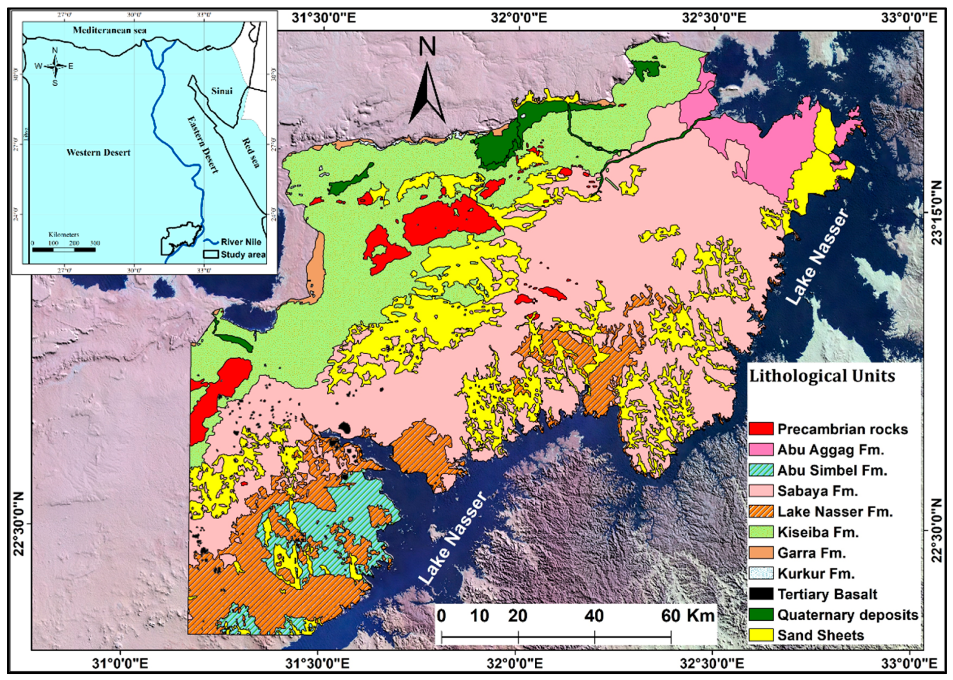
2. Study Area Description

The study area is a part of southern Egypt, located in the southeastern corner of the Egyptian Western Desert, covering an area of 14250 km². It is occupied the area west of Lake Nasser, between latitudes 22°10′–23°40′ N and longitudes 31°10′–33°00′ E, and bounded to the east by the shoreline of the lake (Figure 1).

Geologically, the rock units exposed in the area are from the Precambrian basement to Cenozoic sedimentary successions (Figure 1). The area covered with the Precambrian basement rocks (Arabian Nubian Shield), including granites, granodiorite, gneiss, and Schist [40,41], is overlain by Mesozoic successions of limestones and the Cretaceous sandstones of Abu Agag, Abu Simbel, Sabaya, and Lake Nasser Formations. All of these are covered by Cenozoic rocks of the Tertiary Dakhla, Kiseiba shale, Kurkur, Garra, and Thebes formations; the whole successions are overlain by Quaternary deposits composed of the piedmont gravels, sand sheets, Tufa, and Nile deposits, and are intruded by Oligocene and Quaternary volcanic [42,43,44]. The study site generally belongs to the North Africa arid belt and is characterized by arid conditions with occasional rainfall. These conditions include a long, hot summer and warm winter, where the mean air temperature of the area ranges between 14.2 °C and 38.4 °C.

The Nubian sandstone aquifer in the area represents the principal groundwater aquifer [45]. Over 200 productive wells and piezometers have been drilled, tapping the Sabaya and Abu Simbel Formations of the Nubian Aquifer. It is exposed on the surface of the study region and directly overlies the basement rocks. It is composed of fine to very coarse-grained sandstone with claystone inter-beds. It is hydraulically connected with Lake Nasser water at some localities of the area. The average effective porosity and hydraulic conductivity of this aquifer are 26% and 4.5 m/d, respectively [37,46].

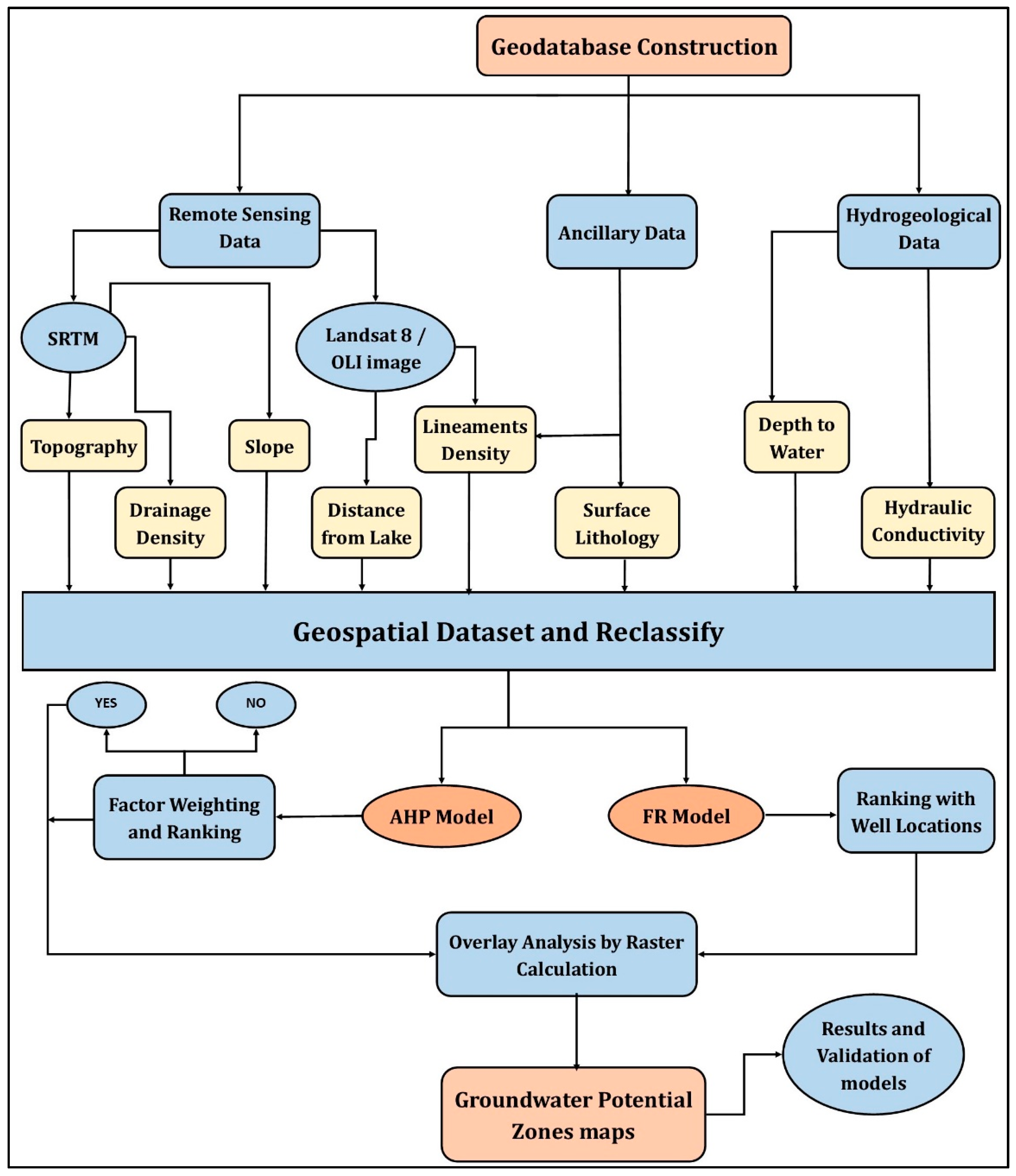
3. Materials and Methods

The groundwater potential zones were delineated by collecting and preparing the spatial database, including thematic layers of the key factors influencing groundwater potentiality, followed by the processing of these layers using the AHP and FR models, and, finally, the interpretation and validation of the results. The methodology of this research is shown in Figure 2.

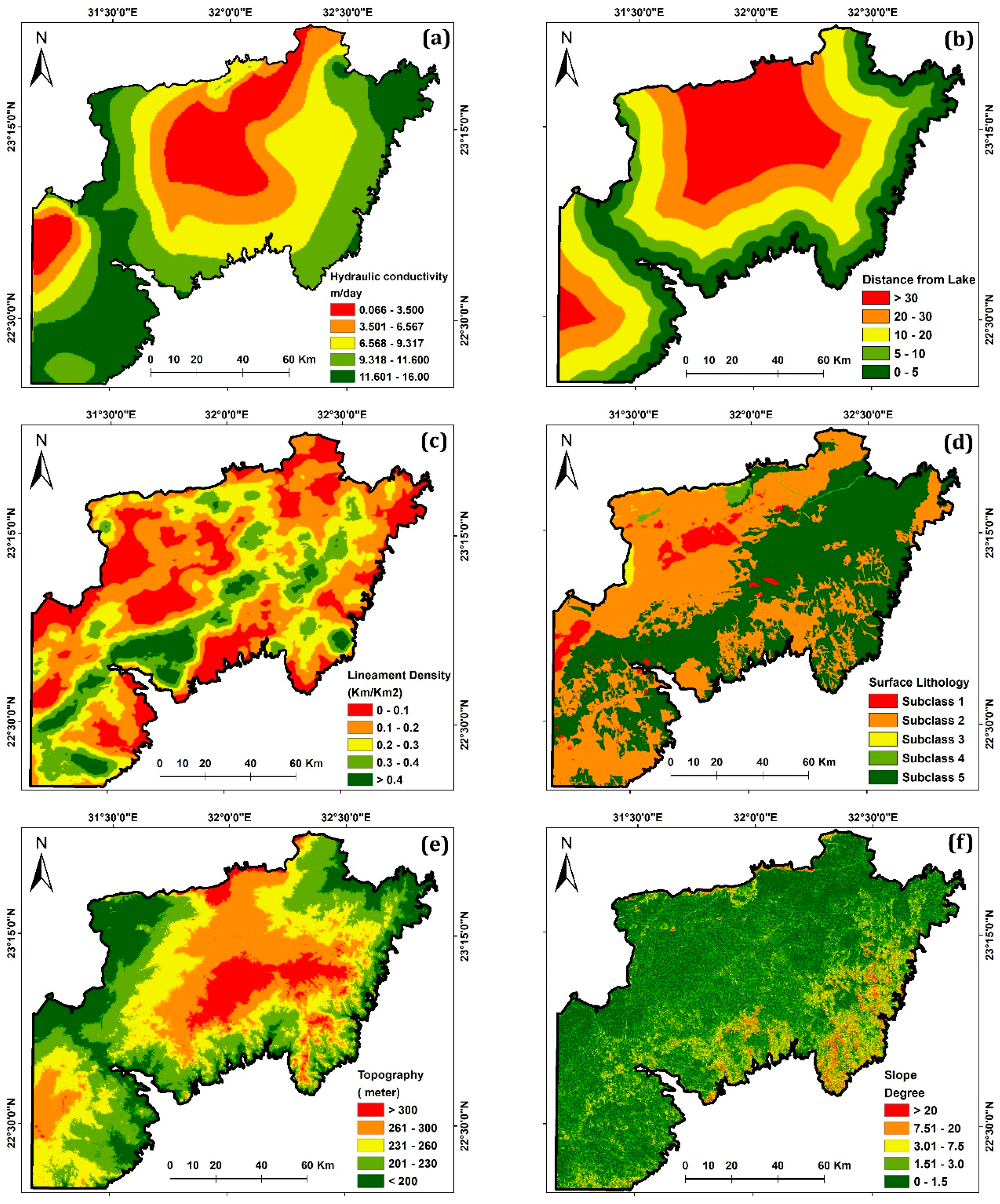
3.1. Thematic Layer Preparation

Eight factors influence the groundwater potentiality in the studied aquifer: hydraulic conductivity, distance from the Lake, lineament density, surface lithology, slope, topography, drainage density, and depth to groundwater. These factors are supposed to control groundwater recharge and groundwater flow in the study area. These factors were processed and presented in the environment of GIS to create the database and apply spatial overlay analysis. Remotely sensed satellite images, hydrogeological data, and maps were provided by governmental institutions and previously published data to generate thematic layers that influence groundwater potentiality.

3.1.1. Hydraulic Conductivity

In general, hydraulic conductivity is an important factor when considering groundwater potentiality, as rock permeability directly affects groundwater flow and storage [47]. Hydraulic conductivity reflects the subsurface lithology of the aquifer and its potentiality, as the higher the permeability, the higher the potentiality. The hydraulic conductivity layer was created from the interpolation of available values resulting from pumping test analysis and based on the previous literature [36,37,48]. The hydraulic conductivity values in the area range from 0.066 to 16 m/day, where the lowest values represent the igneous and metamorphic rocks and highest values represent areas where the sandstone aquifer is dominant. The resultant map of groundwater potentiality was classified and resampled into five classes (Figure 3a).

3.1.2. Distance from the Lake (Lake Nasser)

The Nubian aquifer in the study area is recharged by large quantities of Lake Nasser water, causing an increase in the groundwater level of the aquifer. The detected hypothetical salts in Lake Nasser were the same as those in the Nubian aquifer, indicating the hydraulic connection between the Lake and its adjacent aquifer [37]. Ref. [38] concluded that feeding from Nasser Lake leads to an increase in the groundwater level for a distance up to 30 km from the lake; however, the areas further away from the lake are not affected (during the past 30 years). The distance from the lake layer was extracted using the distance extension and buffer tools in ArcGIS and reclassified into five classes, where the shorter the distance from the lake, the greater possibility of groundwater recharge (Figure 3b).

3.1.3. Lineaments Density

The lineament density reflects rock structures, such as fractures, faults, or joints, denoting a permeable zone that water can infiltrate [49,50]. Therefore, high-groundwater-potential zones are characterized by a high density of lineaments. Lineaments were digitized manually from the geological map of Egypt [39] and were automatically extracted from the Landsat 8 OLI image (Band 8) using PCI Geomatica software (LINE module) [51]. The linear structures were imported and processed into the ArcGIS environment to create a lineament thematic map later used to create the lineament density map in ArcGIS. The lineament density of the study area ranged between 0 and 0.67 km/km², and the area was classified into five classes, as shown in Figure 3c.

3.1.4. Surface Lithology

Surface lithology is a vital factor for groundwater potentiality, as it controls the subsurface flow of groundwater. The lithology layer was digitized from the geological map of Egypt [39]. The lithology of the study area was classified based on its influence on groundwater potentiality into five classes (Figure 3d). Groundwater activities are thought to be lower towards the north and west due to the presence of igneous and metamorphic rocks, owing to the rocks’ low permeability (subclass 1). Granites, granodiorite, and gneiss are considered impermeable units. Although the sedimentary successions represented moderate to high groundwater potential, the sand sheets and clay deposits were considered unsuitable areas for drilling wells (subclass 2). The zones of Nubian sandstone rocks were considered the high potential area of groundwater (subclass 5).

3.1.5. Topography and Slope

Both the topography and slope layers were generated from NASA’s Shuttle Radar Topography Mission (SRTM) with a 30 m resolution using the spatial analysis tool in ArcMap. Before processing the digital elevation model (DEM), a “fill” function was used to eliminate pixel value problems. Because the gravitational forces of the Earth draw water streams down, high-altitude places have a low possibility of groundwater occurrence, and low-altitude regions have a more significant probability [52]. In addition, high-elevation areas are not preferable for drilling wells due to the high cost of water extraction. The elevation of the study area ranges from 135 to 459 m.a.s.l (Figure 3e). The highly elevated areas are located in the middle region of the study area, while low-land areas are spread around the outskirts of the area, especially near the lake. The study area was reclassified into five topographic classes, as shown in Figure 3e.

Slope angle has a significant impact, as the slope determines how much surface water percolates into the groundwater [13]. The steeper the slope, the lower the infiltration rate will be due to the more considerable runoff potential [53]. The slope map was reclassified into five classes (Figure 3f), where high weight was given to flat and gentle slopes, and low weight was given to steep slopes.

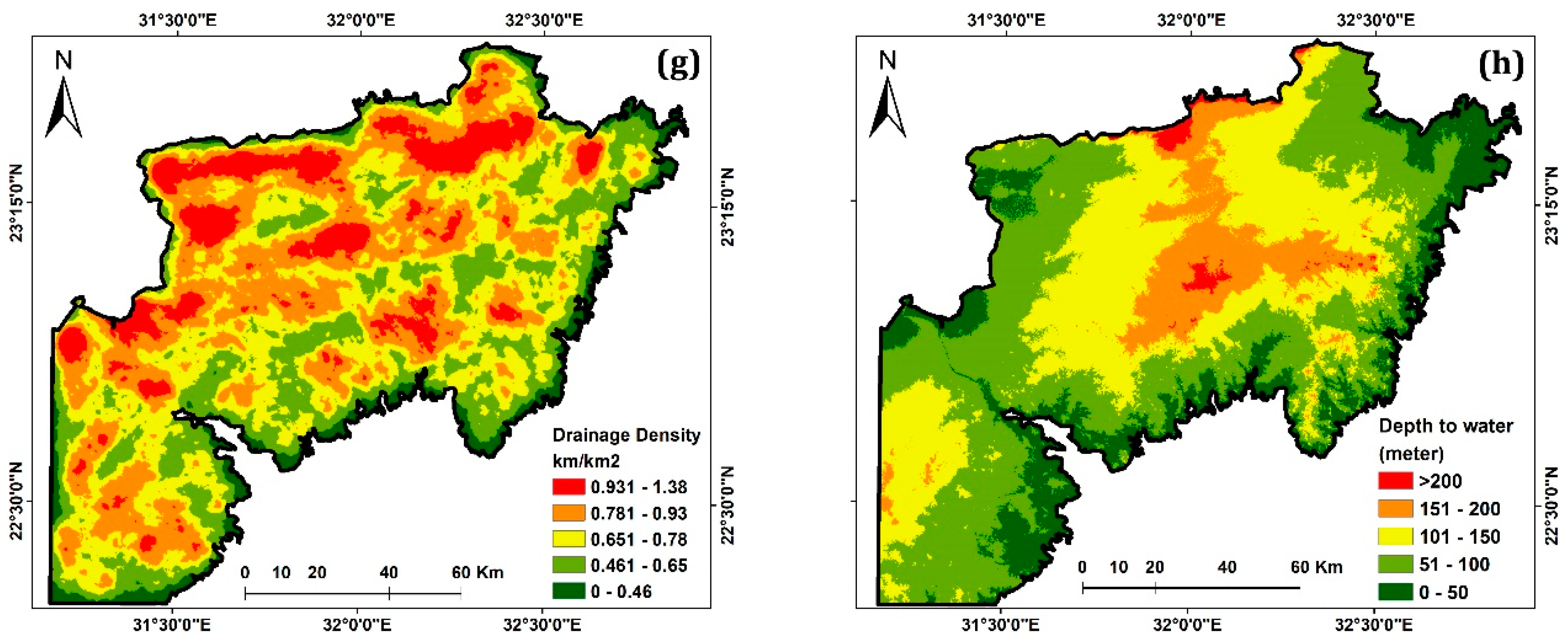
3.1.6. Drainage Density

The drainage density is linked to the infiltration rate, with high drainage density representing less infiltration. The drainage density is obtained mathematically by dividing the total lengths of all the streams in a drainage basin by the drainage basin’s total area. The drainage density map was prepared from the drainage map using the ArcGIS platform (line density tool) (Figure 3g). The density values of the study area ranged between 0 and 1.38 km/km². However, for groundwater potentiality, high weight was attributed to low drainage density and low weight was assigned to high drainage density.

3.1.7. Depth to Water

The depth to groundwater is defined as the vertical distance from the ground’s surface to the static water level. It measures the potential distance for water to travel to the aquifer and controls the cost of water consumption and abstraction. In general, the deeper the water is, the lower the potentiality of groundwater. Water level measurement data from 44 boreholes during December 2018 were used to prepare the depth to water map of the area shown in Figure 3h. The inverse distance-weighted (IDW) interpolation method of the spatial analysis tool in ArcGIS was used to fill the gaps in null data areas. Depth to water exhibited significant variations in the study area; it ranged between 4 and 258 m. The depth to water map was classified into five classes from 1 to 5, representing potentiality classes from high to low, respectively (Figure 3h).

3.2. Analytical Hierarchy Process (AHP) Method

The groundwater potential zones in the AHP model were classified based on the index value calculated using Equation (1):

$$\mathrm{GWPI}={\mathrm{C}}_{\mathrm{w}}{\mathrm{C}}_{\mathrm{r}}+{\mathrm{D}}_{\mathrm{w}}{\mathrm{D}}_{\mathrm{r}}+{\mathrm{Ld}}_{\mathrm{w}}{\mathrm{Ld}}_{\mathrm{r}}+{\mathrm{G}}_{\mathrm{w}}{\mathrm{G}}_{\mathrm{r}}+{\mathrm{T}}_{\mathrm{w}}{\mathrm{T}}_{\mathrm{r}}+{\mathrm{S}}_{\mathrm{w}}{\mathrm{S}}_{\mathrm{r}}+{\mathrm{Dd}}_{\mathrm{w}}{\mathrm{Dd}}_{\mathrm{r} }+{\mathrm{Sw}}_{\mathrm{w}}{\mathrm{Sw}}_{\mathrm{r} }{}_{ }$$

(1)

where GWPI is the groundwater potential zone index, C is the hydraulic conductivity, G is the surface lithology (geology), D is the distance from the Lake, Ld donates the lineament density, T refers to topography, S is the slope, Dd is drainage density, Sw is the static water or depth to water, (w) is the weight, and (r) is the rate of each factor.

The weight of each factor (w) was determined using the AHP model through two main steps. The first step is the construction of a pair-wise comparison matrix between all of the (eight) influencing factors [54]. The relative importance of each parameter on groundwater potentiality was graded according to Saaty’s 1–9 scale [9]. The rank of 9 was given to criteria that have an extremely strong influence over the other, while a rank of 1 meant equal significance for the two compared parameters.

The relevance of each factor was determined based on the review of past studies, field experience, and expert’s opinions. Accordingly, in the pair-wise comparison matrix, all concerned parameters were graded compared with each other (

Table 1. Pair-wise comparison matrix between the applied parameters for the AHP model.

	Hydraulic Conductivity	Distance from Lake	Lineament Density	Surface Lithology	Topography	Slope	Drainage Density	Static Water Level
Hydraulic Conductivity	1	2	2	3	4	5	5	6
Distance from Lake	½	1	2	3	3	4	4	5
Lineament Density	½	½	1	2	2	3	3	4
Surface Lithology	⅓	⅓	½	1	2	3	3	4
Topography	¼	⅓	½	½	1	2	1	2
Slope	⅕	¼	⅓	⅓	½	1	1	2
Drainage Density	⅕	¼	⅓	⅓	1	1	1	2
Static Water Level	⅙	⅕	¼	¼	½	½	½	1
Sum	3.15	4.87	6.92	10.42	14.00	19.50	18.50	26.00

). In the next step, the normalized pair-wise comparison matrix was created by dividing each cell by the sum of each column, and normalized weights for each component were calculated using the average of each row (

Table 2. Normalized pair-wise comparison matrix and weights of each factor.

	Hydraulic Conductivity	Distance from Lake	Lineament Density	Surface Lithology	Topography	Slope	Drainage Density	Static Water Level	Weights
Hydraulic Conductivity	0.317	0.411	0.289	0.288	0.286	0.256	0.270	0.231	0.294
Distance from Lake	0.159	0.205	0.289	0.288	0.214	0.205	0.216	0.192	0.221
Lineament Density	0.159	0.103	0.145	0.192	0.143	0.154	0.162	0.154	0.151
Surface Lithology	0.106	0.068	0.072	0.096	0.143	0.154	0.162	0.154	0.119
Topography	0.079	0.068	0.072	0.048	0.071	0.103	0.054	0.077	0.072
Slope	0.063	0.051	0.048	0.032	0.036	0.051	0.054	0.077	0.052
Drainage Density	0.063	0.051	0.048	0.032	0.071	0.051	0.054	0.077	0.056
Static Water Level	0.053	0.041	0.036	0.024	0.036	0.026	0.027	0.038	0.035
Sum	1.000	1.000	1.000	1.000	1.000	1.000	1.000	1.000	1.000

).

The created matrix was checked for consistency by determining the consistency ratio (CR) using Equations (2) and (3) developed by [55].

$$\mathrm{CR}=\frac{\mathrm{CI}}{\mathrm{RI}}$$

(2)

$$\mathrm{CI}=\frac{\mathsf{\lambda }\max -\mathrm{n}}{\mathrm{n}-1}$$

(3)

where RI is the random index obtained from Saaty’s standard (

Table 3. Random consistency index (RI) introduced by [9].

Less Importance								More Importance
RI	0	0	0.58	0.9	1.12	1.24	1.32	1.41	1.45	1.49	1.51
n	1	2	3	4	5	6	7	8	9	10	11

), determined by the number of criteria, which in this study was equal to 1.41; CI is the consistency index; where λmax is the principal eigenvalue of the matrix, which is equal to 8.19; and n is the number of parameters applied in the matrix, which was equal to 8 in the present study.

Refs. [54,55] stated that the model prediction can be accepted and reliable if the CR is less than or equal to 0.1%. However, if the CR is higher than (0.1), the prediction model needs to be reassessed.

All factors were classified into subclasses and ranked based on their influence on groundwater potentiality. The lowest grade was given to the class with the most minor influence, and the highest was given to the class with the strongest influence. Finally, the normalized rate I of each subclass was determined by dividing each rank value by the total of all rankings for each factor, as shown in

Table 4. Assigned normalized weights and rates for all factors and subclasses.

No.	Factors	Subclasses	Rating	Weights
1	Hydraulic conductivity	0.066–3.5	0.053	0.294
		3.5–6.567	0.158
		6.567–9.318	0.211
		9.318–11.6	0.263
		11.6–16.00	0.316
2	Distance from Lake	0–5	0.316	0.221
		5–10	0.263
		10–20	0.211
		20–30	0.158
		>30	0.053
3	Lineament Density	0–0.1	0.067	0.151
		0.1–0.2	0.133
		0.2–0.3	0.200
		0.3–0.4	0.267
		>0.4	0.333
4	Surface lithology	Igneous and Metamorphic rocks	0.059	0.119
		Clay, claystone, fine sandstone, and sand sheets	0.118
		Limestone of Kurukur and Garra Fms.	0.176
		Wadi and Quaternary deposits	0.294
		Nubian Sandstone and Gravels	0.353
5	Topography	<200	0.353	0.072
		200–230	0.294
		230–260	0.176
		260–300	0.118
		>300	0.059
6	Slope	0–1.5	0.333	0.052
		5–3	0.267
		3–7.5	0.200
		7.5–20	0.133
		>20	0.067
7	Drainage Density	<0.46	0.333	0.056
		0.46–0.65	0.267
		0.65–0.78	0.200
		0.78–0.93	0.133
		0.93–1.38	0.067
8	Static water level	0–50	0.353	0.035
		50–100	0.294
		100–150	0.176
		150–200	0.118
		>200	0.059

. In the AHP method, the groundwater potential map was constructed by overlaying the obtained controlling factors (thematic layers), which were calculated from Equation (1), using ArcMap 10.7.1.

3.3. Frequency Ratio (FR) Method

The frequency ratio (FR) model is a bivariate statistical approach used as a valuable technique for geospatial evaluation to examine the probability connection between independent and dependent data, such as multi-classified maps [56]. It has recently been utilized to map groundwater potential in a specific place based on the link between the observed pumping wells and parameters regulating groundwater potential [18,21,57]. In this method, an FR value should be assigned for each subclass of the groundwater influencing parameter using Equation (4) [56]:

$$\mathrm{FR}=\frac{\mathrm{W}/\mathrm{G}}{\mathrm{M}/\mathrm{T}}$$

(4)

where W is the number of groundwater wells representing each conditioning factor’s subclass, G is the total number of groundwater wells in the study area, M is the number of pixels representing the subclass of the factor, and T is the total number of pixels in the study area.

In this study, 44 groundwater pumping wells were used, and the FR value for each subclass of used parameters was calculated and is presented in

Table 5. The spatial relationship between the factors and wells with the assigned FR for each subclass.

No.	Factors	Subclasses	No. of Pixels	Percentage of Subclass	No. of Wells	Percentage of Wells	FR
1	Hydraulic conductivity	0.066–3.5	210,565	14.70	0	0.00	0.000
		3.5–6.567	227,811	15.91	1	2.27	0.143
		6.567–9.318	338,147	23.61	3	6.82	0.289
		9.318–11.6	339,749	23.72	11	25.00	1.054
		11.6–16.00	315,848	22.05	29	65.91	2.988
2	Distance from Lake	0–5	281,709	19.63	20	45.45	2.316
		5–10	227,445	15.85	17	38.64	2.438
		10–20	371,659	25.89	5	11.36	0.439
		20–30	259,197	18.06	2	4.55	0.252
		>30	295,346	20.58	0	0.00	0.000
3	Lineament Density	0–0.1	346,082	24.11	15	34.09	1.414
		0.1–0.2	487,932	34.00	9	20.45	0.602
		0.2–0.3	329,150	22.93	7	15.91	0.694
		0.3–0.4	193,369	13.47	7	15.91	1.181
		>0.4	78,730	5.49	6	13.64	2.486
4	Surface lithology	Ign. And Meta. Rocks	52,600	3.66	0	0.00	0.000
		Clays, fine s.s, and sand sheets	697,457	48.59	17	38.64	0.795
		L.S of Kurukur and Garra Fms.	17,444	1.22	3	6.82	5.610
		Wadi and Qs. Deposits	13,411	0.93	0	0.00	0.000
		Nubian S.S and Gravels	654,459	45.60	24	54.55	1.196
5	Topography	<200	276,288	19.25	21	47.73	2.479
		200–230	384,425	26.78	19	43.18	1.612
		230–260	356,523	24.84	4	9.09	0.366
		260–300	307,777	21.44	0	0.00	0.000
		>300	110,307	7.69	0	0.00	0.000
6	Slope	0–1.5	729,970	51.13	24	54.55	1.067
		5–3	545,889	38.23	18	40.91	1.070
		3–7.5	106,144	7.43	2	4.55	0.611
		7.5–20	32,691	2.29	0	0.00	0.000
		>20	13,106	0.92	0	0.00	0.000
7	Drainage Density	<0.46	927,935	6.47	0	0.00	0.000
		0.46–0.65	3,121,085	21.75	19	43.18	1.986
		0.65–0.78	4,592,402	32.00	7	15.91	0.497
		0.78–0.93	4,046,225	28.19	13	29.55	1.048
		0.93–1.38	1,664,497	11.60	5	11.36	0.980
8	Static water level	0–50	232,236	16.18	15	34.09	2.107
		50–100	573,308	39.95	25	56.82	1.422
		100–150	454,686	31.68	4	9.09	0.287
		150–200	156,139	10.88	0	0.00	0.000
		>200	18,782	1.31	0	0.00	0.000

. The GWPI map was constructed following the FR method by integrating the FR layers of the controlling factors (thematic layers) (Equation (5)) using ArcMap 10.7.1.

$$\mathrm{GWPI}={\sum }_{\mathrm{i}=1}^{\mathrm{n}}\mathrm{FR}$$

(5)

4. Results

The groundwater potential zones were estimated based on the AHP and FR models, considering the previously mentioned methodology applied to the eight most influential thematic layers.

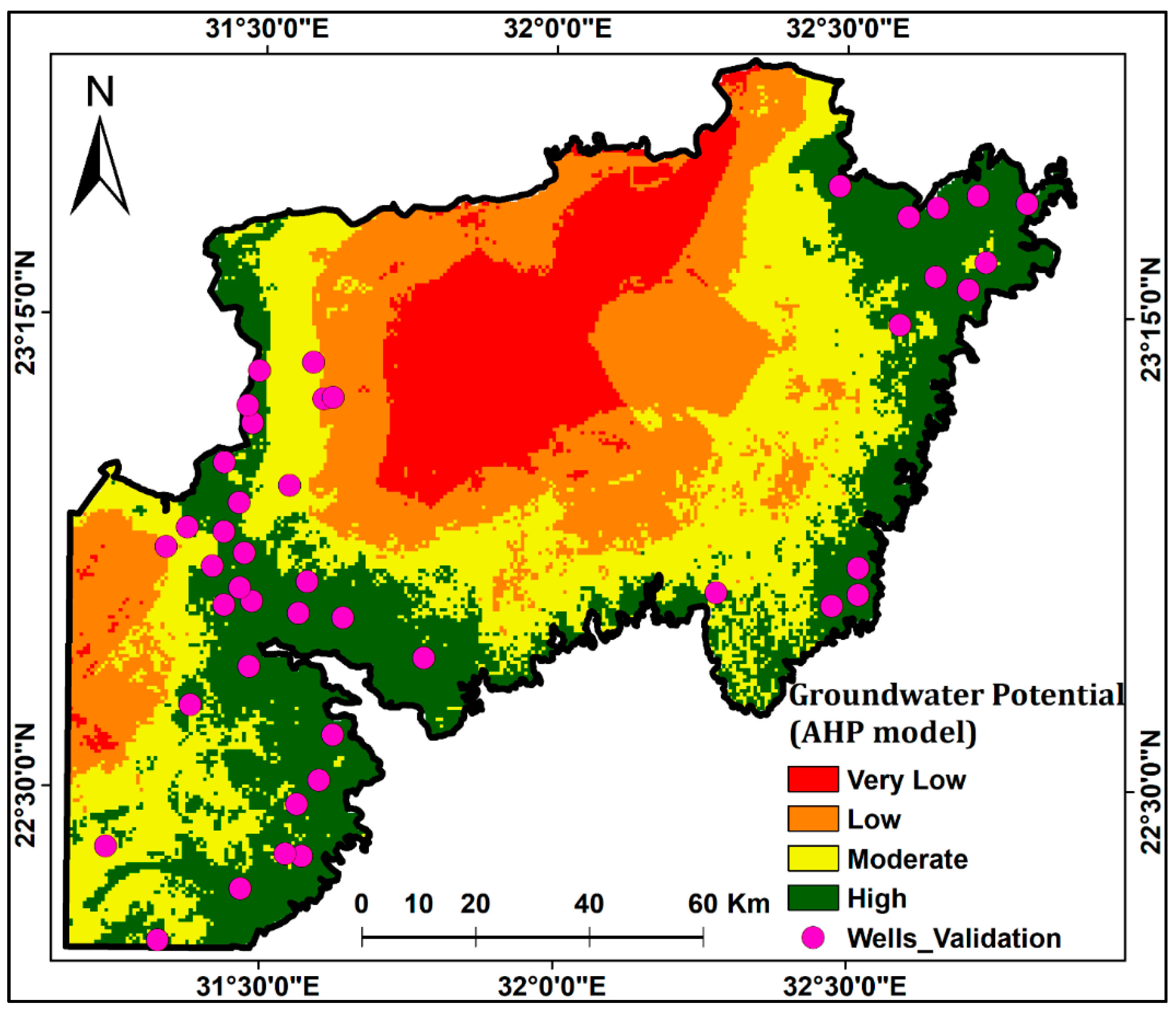
4.1. Results of AHP Model

In the AHP model, the final weight of each influencing feature is shown in Table 4. From the pair-wise comparison results, the most weight was given to the hydraulic conductivity, distance from the Lake, lineament density, and surface lithology factors.. The CR was 0.0197, reflecting a good level of consistency in the pair-wise comparison phase. The resulting groundwater potential map obtained by the AHP model is shown in Figure 4, and was classified based on the natural breaks classification method in ArcGIS into four classes: high, moderate, low, and very low categories. In this map, most of the study area was classified as moderate potential (31.4%), 29.4% of the total area was classified as high, 25.8% as low, and 13.4% as very low groundwater potentiality.

4.2. Results of FR Model

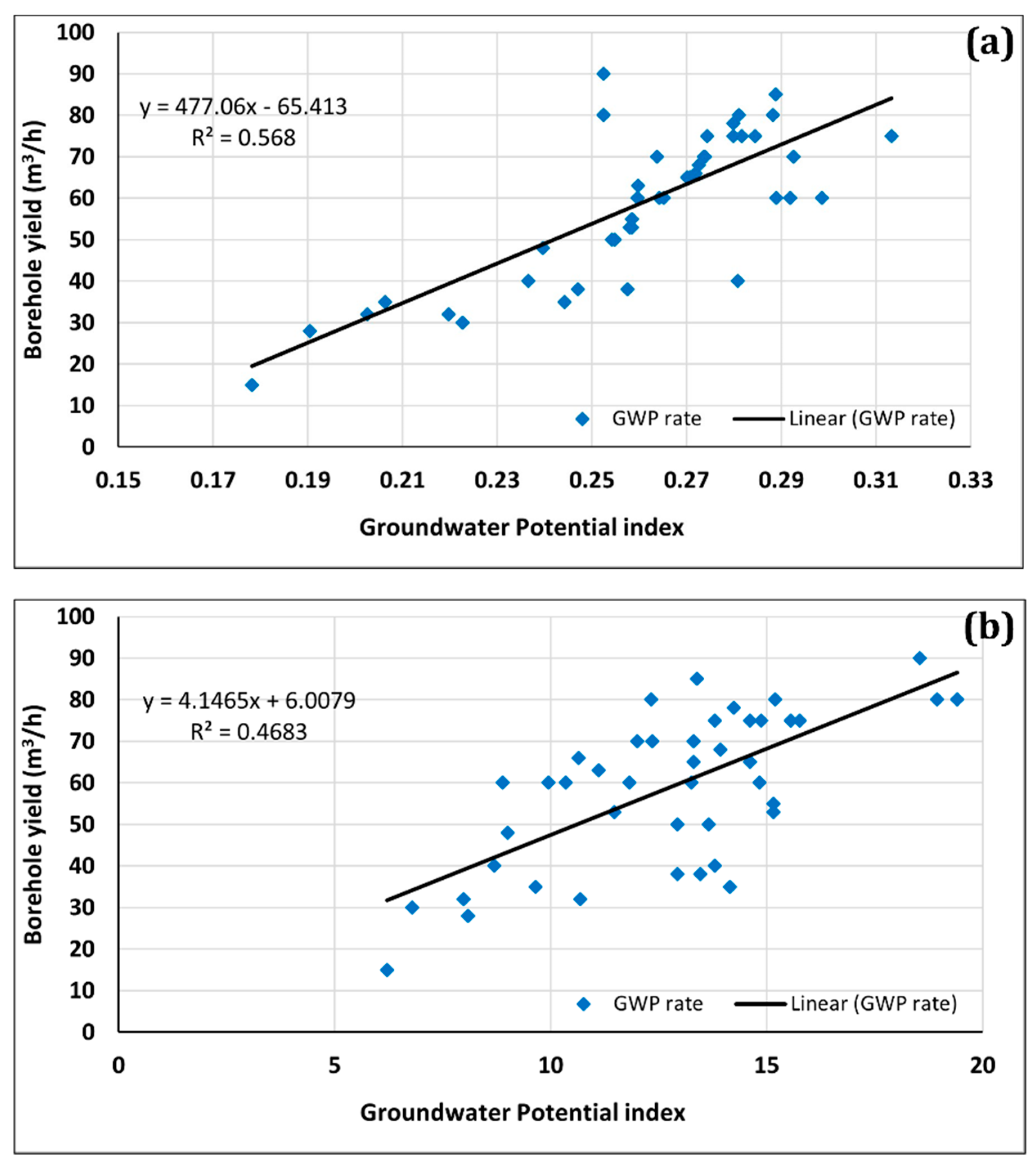
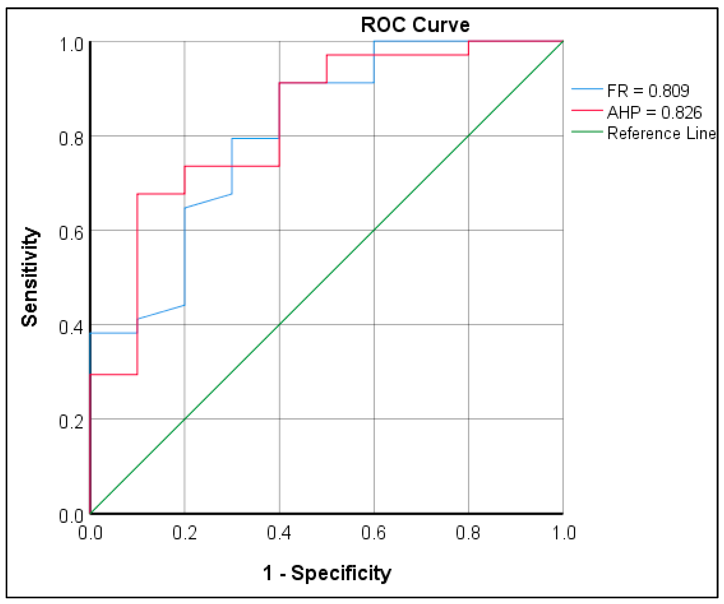
According to relationships between the pumping well and each conditioning factor, the FR model was applied, and the results are shown in Table 5. An FR value of 1 implies an average geographical correlation between the location of a groundwater well and its conditioning parameter. There is a low correlation if the value is less than 1 and a stronger correlation if the value is greater than 1 [58].

The spatial relationships between the groundwater wells and hydraulic conductivity values revealed a low possibility of groundwater potential in the range of hydraulic conductivity below 9.32 m/day. Areas with distances less than 10 km from the lake had a high probability of groundwater potential, with FR values of >2. The calculations showed that as the distance from the lake increased, the ratio decreased. Additionally, the assessment of the lineament density indicated that density classes of >0.4 km/km² had the highest value of FR (2.49), followed by 0–0.1 classes (1.414). The lowest FR (0.6) value was defined for 0.1–0.2 classes. Limestone of the Kurkur and Garra Formations class had the highest value of FR (5.6) due to the limitation of that type of surface rock in the region with the presence of three pumping wells in that class, followed by the sandstone and gravel deposits class (FR = 1.2), in which most of the pumping wells were drilled in the region. The igneous and metamorphic rocks acting as an aquifuge had an FR value of zero. In case of topography, the FR values reflected a decrease in groundwater potential as the altitude increased. Similarly, the FR values were inversely proportional to the slope angle (Table 5). The locations with drainage densities of 0.46–0.65 and 0.78–0.93 km/km² possessed the highest frequency ratio (FR = 1.99, 1.05, respectively), reflecting the strong relationship with groundwater potentiality. The static water level factor showed that the regions with the lowest static water levels (0–50 m) had the maximum frequency ratio (2.11). The groundwater potential map produced by the FR model is shown in Figure 5, which was reclassified based on the natural breaks classification method into four classes: high potential (23.4%), moderate potential (28.2%), low potential (25.3%), and very low potential (23.1%).

4.3. Validation

The validation of the results is necessary to acquire trust in the spatial approaches developed in this work and to identify their physical relevance. In the present study, the groundwater potential zone maps were validated by the overlying number of productive wells on the map (Figure 4 and Figure 5), considering that most of these wells were pumped with a high yield.

The overlying and extraction processes within ArcGIS were performed to assume the potential zone of each well. A total of 44 existing pumping wells were identified in the study area. In the AHP method, no wells were found to be in the very low groundwater potential zone (GWPZ), only two wells were found to exist within the poor GWPZ, and 36 wells were found within the high GWPZ (

Table 6. The distribution of groundwater potential classes based on the AHP and FR models.

	AHP Model				FR Model
	Range	Area (km2)	Area%	Pumping Wells	Range	Area (km2)	Area%	Pumping Wells
Very Low	0.0787–0.142	1906.24	13.43	0	0.891–4.701	3275.38	23.07	0
Low	0.142–0.196	3662.00	25.80	2	4.701–7.38	3592.61	25.31	2
Moderate	0.196–0.242	4452.89	31.37	6	7.38–10.65	4004.96	28.21	9
High	0.242–0.3167	4174.97	29.41	36	10.65–20.09	3323.26	23.41	33

), indicating a high level of validation. Likewise, only 2 of these 44 wells existed within the very poor and poor GWPZ in the FR method, and 33 wells were located within the high GWPZ. Therefore, the model was valid, as it indicated that 82% and 75% of wells existed in the high GWPZ for the AHP and FR models, respectively.

The yield of the groundwater wells was compared to the groundwater potential index calculated using the AHP and FR models. The groundwater yield values varied from 15 to 28, 30–48, and 38–90 m³/h in the low, moderate, and high-potential zones using the AHP model, respectively; while, for the FR model, they varied from 15–30, 28–70, and 32–90 m³/h in the low, moderate, and high-potential zones, respectively. The scatter plot between the groundwater potential index and well yield values showed a reasonable correlation, with coefficient of determination (R²) values equal to 0.57 and 0.47 for the AHP and FR models (Figure 6a,b), respectively. This demonstrates that the AHP model was a good model for describing zones of good groundwater yield, since it described borehole yield variability around its mean.

Moreover, the ROC curve was prepared by comparing the existing groundwater well locations in the validation datasets with the groundwater potential map [1,59].

The ROC curve of the GPMZs generated using the AHP and FR models is shown in Figure 7. These graphs showed that the AHP model (AUC = 82.6%) outperformed the FR model (AUC = 80.9%).

Based on [21], the AUC values corresponding to the prediction accuracy were divided into poor (0.5–0.6), average (0.6–0.7), good (0.7–0.8), very good (0.8, 0.9), and excellent (0.9–1). As a consequence of these validation results, the AHP and FR models used in this work both exhibited reasonable accuracy in spatial groundwater potential prediction, with the AHP technique being more efficient than the FR model in this study.

5. Discussion

The groundwater potentiality in a semi-arid area surrounding Nasser Lake was mapped using the integration of GIS, remote sensing, and multi-criteria decision analysis AHP and FR. In such areas characterized by rain scarcity, factors controlling subsurface recharge are predominant, and the influence of the factors controlling the vertical seepage from the surface is lower [60]. In the area surrounding Lake Nasser, where lake water feeds the groundwater aquifer, the factors controlling groundwater flow, such as hydraulic conductivity, proximity to the lake, and lineament density have the greatest impact. The normalized matrix (Table 4) revealed that hydraulic conductivity was the most significant factor, accounting for 29.4%, followed by the distance from Lake Nasser, at 22.1%, while the slope and static water level were the least influential at 5.2% and 3.5%, respectively.

On the contrary, [13,60,61] concluded that lithology (geology), slope, and rainfall are the main influential factors of groundwater potential using the AHP model in the Vaitarna Basin of India, Motloutse Watershed of Botswana, and Tirnavos area of Greece, respectively. This is because groundwater recharge in these areas depends mainly on rainfall and recharge from flood water, while in the area west of Lake Nasser, where there is very little rainfall, recharge from Lake water prevails.

The resultant maps constructed using the AHP and FR techniques showed that the high-potential zones were located close to Lake Nasser due to the high hydraulic conductivity of the subsurface rocks, proximity to the lake, and permeable surface lithology in these areas. Furthermore, due to the low permeability, high altitudes, and steep slopes, the central part of the research site fell within very low groundwater potential zones.

Despite the high matching between the maps resulting from both AHP and FR, the spatial pattern of some zones differed somewhat. This difference may be related to the location of the pumping wells drilled in the observed low and moderate-potential zones, which increased the calculated potentiality of these areas in the FR technique.

One of the most important limitations in this study was the lack of data. Interpolation methods were used to compensate for the lack of that data to cover the entire study area. Future studies should be carried out to fill this gap in data, especially the lineament characteristics, hydraulic conductivity, and groundwater levels. Overall, the produced groundwater potential maps indicated reliable potentiality for groundwater occurrence. Accordingly, the potential areas can be easily identified on the produced maps and they can be used by the decision-makers to locate drilling sites in the ongoing reclamation projects during that period. They will be useful to avoid the wasted cost of drilling unproductive and unsustainable wells.

6. Conclusions

The southern part of Egypt is experiencing arid conditions and a significant increase in water demands due to reclamation projects. Consequently, assessing and evaluating the groundwater potentiality west of Lake Nasser can provide highly beneficial results for water resource management. There have been no studies on the southern parts of Egypt using approaches such as MCDA. Therefore, AHP and FR were used to carry out the present work to assess groundwater potential zones. In this study, an attempt was made using eight groundwater controlling factors to develop a groundwater potential zone map. The study showed that the high and moderate-potential zones were 61% to 52% of the total area for AHP and FR, respectively. Therefore, the results indicated that 82% and 75% of wells existed in the high GWPZ for the AHP and FR models, respectively. The performance and validation of the employed models were conducted using the ROC curve. The ROC curve accuracy for both employed approaches, i.e., AHP and FR, revealed accuracy values of 83% and 81%, indicating a better predictive performance rate for the AHP approach.

The AHP and FR-based approaches for delineating groundwater potential zones used in this study were effective due to their ability to generate reliable results that could be applied in the development of semi-arid regions, especially in developing and low-income countries. It can be argued that the complexity and highly dynamic nature of the relationship between the lake and adjacent aquifer, the lineament characteristics, aquifer hydraulic parameters, and fluctuation of water levels in both systems, making it is necessary to conduct monitoring and integrating water levels in future studies.

References

1. Pradhan, B. Groundwater potential zonation for basaltic watersheds using satellite remote sensing data and GIS techniques. Cent. Eur. J. Geosci. 2009, 1, 120–129. [Google Scholar] [CrossRef]
2. Al-Shabeeb, A.A.R.; Al-Adamat, R.; Al-Fugara, A.; Al-Amoush, H.; AlAyyash, S. Delineating groundwater potential zones within the Azraq Basin of Central Jordan using multi-criteria GIS analysis. Groundw. Sustain. Dev. 2018, 7, 82–90. [Google Scholar] [CrossRef]
3. Jasrotia, A.S.; Kumar, R.; Saraf, A.K. Delineation of groundwater recharge sites using integrated remote sensing and GIS in Jammu district, India. Int. J. Remote Sens. 2007, 28, 5019–5036. [Google Scholar] [CrossRef]
4. Hammouri, N.; Al-Amoush, H.; Al-Raggad, M.; Harahsheh, S. Groundwater recharge zones mapping using GIS: A case study in Southern part of Jordan Valley, Jordan. Arab. J. Geosci. 2014, 7, 2815–2829. [Google Scholar] [CrossRef]
5. Kumar, P.K.D.; Gopinath, G.; Seralathan, P. Application of remote sensing and GIS for the demarcation of groundwater potential zones of a river basin in Kerala, southwest coast of India. Int. J. Remote Sens. 2007, 28, 5583–5601. [Google Scholar] [CrossRef]
6. Das, S.; Pardeshi, S.D. Integration of different influencing factors in GIS to delineate groundwater potential areas using IF and FR techniques: A study of Pravara basin, Maharashtra, India. Appl. Water Sci. 2018, 8, 197. [Google Scholar] [CrossRef] [Green Version]
7. Das, S.; Gupta, A.; Ghosh, S. Exploring groundwater potential zones using MIF technique in semi-arid region: A case study of Hingoli district, Maharashtra. Spat. Inf. Res. 2017, 25, 749–756. [Google Scholar] [CrossRef]
8. Magesh, N.S.; Chandrasekar, N.; Soundranayagam, J.P. Delineation of groundwater potential zones in Theni district, Tamil Nadu, using remote sensing, GIS and MIF techniques. Geosci. Front. 2012, 3, 189–196. [Google Scholar] [CrossRef] [Green Version]
9. Saaty, T.L. What is the analytic hierarchy process. In Mathematical Models for Decision Support; Springer: Berlin/Heidelberg, Germany, 1988; pp. 109–121. [Google Scholar]
10. Agarwal, E.; Agarwal, R.; Garg, R.D.; Garg, P.K. Delineation of groundwater potential zone: An AHP/ANP approach. J. Earth Syst. Sci. 2013, 122, 887–898. [Google Scholar] [CrossRef] [Green Version]
11. Jenifer, M.A.; Jha, M.K. Comparison of Analytic Hierarchy Process, Catastrophe and Entropy techniques for evaluating groundwater prospect of hard-rock aquifer systems. J. Hydrol. 2017, 548, 605–624. [Google Scholar] [CrossRef]
12. Rahmati, O.; Nazari Samani, A.; Mahdavi, M.; Pourghasemi, H.R.; Zeinivand, H. Groundwater potential mapping at Kurdistan region of Iran using analytic hierarchy process and GIS. Arab. J. Geosci. 2015, 8, 7059–7071. [Google Scholar] [CrossRef]
13. Das, S. Comparison among influencing factor, frequency ratio, and analytical hierarchy process techniques for groundwater potential zonation in Vaitarna basin, Maharashtra, India. Groundw. Sustain. Dev. 2019, 8, 617–629. [Google Scholar] [CrossRef]
14. Mohammadi-Behzad, H.R.; Charchi, A.; Kalantari, N.; Nejad, A.M.; Vardanjani, H.K. Delineation of groundwater potential zones using remote sensing (RS), geographical information system (GIS) and analytic hierarchy process (AHP) techniques: A case study in the Leylia–Keynow watershed, southwest of Iran. Carbonates Evaporites 2019, 34, 1307–1319. [Google Scholar] [CrossRef]
15. Arulbalaji, P.; Padmalal, D.; Sreelash, K. GIS and AHP Techniques Based Delineation of Groundwater Potential Zones: A case study from Southern Western Ghats, India. Sci. Rep. 2019, 9, 2082. [Google Scholar] [CrossRef]
16. Yu, Y.; Wu, Y.; Yu, N.; Wan, J. Fuzzy comprehensive approach based on AHP and entropy combination weight for pipeline leak detection system performance evaluation. In Proceedings of the 2012 IEEE International Systems Conference, Vancouver, BC, Canada, 19–22 March 2012; pp. 606–611. [Google Scholar]
17. Waris, M.; Panigrahi, S.; Mengal, A.; Soomro, M.I.; Mirjat, N.H.; Ullah, M.; Azlan, Z.S.; Khan, A. An Application of Analytic Hierarchy Process (AHP) for Sustainable Procurement of Construction Equipment: Multicriteria-Based Decision Framework for Malaysia. Math. Probl. Eng. 2019, 2019, 6391431. [Google Scholar] [CrossRef]
18. Guru, B.; Seshan, K.; Bera, S. Frequency ratio model for groundwater potential mapping and its sustainable management in cold desert, India. J. King Saud Univ. Sci. 2017, 29, 333–347. [Google Scholar] [CrossRef] [Green Version]
19. Trabelsi, F.; Lee, S.; Khlifi, S.; Arfaoui, A. Frequency Ratio Model for Mapping Groundwater Potential Zones Using GIS and Remote Sensing; Medjerda Watershed Tunisia; Springer: Cham, Switzerland, 2019; pp. 341–345. [Google Scholar]
20. Ahmadi, H.; Kaya, O.A.; Babadagi, E.; Savas, T.; Pekkan, E. GIS-Based Groundwater Potentiality Mapping Using AHP and FR Models in Central Antalya, Turkey. Environ. Sci. Proc. 2020, 5, 8741. [Google Scholar] [CrossRef]
21. Razandi, Y.; Pourghasemi, H.R.; Neisani, N.S.; Rahmati, O. Application of analytical hierarchy process, frequency ratio, and certainty factor models for groundwater potential mapping using GIS. Earth Sci. Inform. 2015, 8, 867–883. [Google Scholar] [CrossRef]
22. Abu El-Magd, S.A.; Embaby, A. To investigate groundwater potentiality, a GIS-based model was integrated with remote sensing data in the Northwest Gulf of Suez (Egypt). Arab. J. Geosci. 2021, 14, 2737. [Google Scholar] [CrossRef]
23. Lee, S.; Kim, Y.S.; Oh, H.J. Application of a weights-of-evidence method and GIS to regional groundwater productivity potential mapping. J. Environ. Manag. 2012, 96, 91–105. [Google Scholar] [CrossRef]
24. Sahoo, S.; Munusamy, S.B.; Dhar, A.; Kar, A.; Ram, P. Appraising the Accuracy of Multi-Class Frequency Ratio and Weights of Evidence Method for Delineation of Regional Groundwater Potential Zones in Canal Command System. Water Resour. Manag. 2017, 31, 4399–4413. [Google Scholar] [CrossRef]
25. Rahmati, O.; Kornejady, A.; Samadi, M.; Nobre, A.D.; Melesse, A.M. Development of an automated GIS tool for reproducing the HAND terrain model. Environ. Model. Softw. 2018, 102, 1–12. [Google Scholar] [CrossRef]
26. Rahmati, O.; Naghibi, S.A.; Shahabi, H.; Bui, D.T.; Pradhan, B.; Azareh, A.; Rafiei-Sardooi, E.; Samani, A.N.; Melesse, A.M. Groundwater spring potential modelling: Comprising the capability and robustness of three different modeling approaches. J. Hydrol. 2018, 565, 248–261. [Google Scholar] [CrossRef]
27. Rahmati, O.; Melesse, A.M. Application of Dempster–Shafer theory, spatial analysis and remote sensing for groundwater potentiality and nitrate pollution analysis in the semi-arid region of Khuzestan, Iran. Sci. Total Environ. 2016, 568, 1110–1123. [Google Scholar] [CrossRef]
28. Abu El-Magd, S.A.; Eldosouky, A.M. An improved approach for predicting the groundwater potentiality in the low desert lands; El-Marashda area, Northwest Qena City, Egypt. J. Afr. Earth Sci. 2021, 179, 104200. [Google Scholar] [CrossRef]
29. Hou, E.; Wang, J.; Chen, W. A comparative study on groundwater spring potential analysis based on statistical index, index of entropy and certainty factors models. Geocarto Int. 2018, 33, 754–769. [Google Scholar] [CrossRef]
30. Ozdemir, A. GIS-based groundwater spring potential mapping in the Sultan Mountains (Konya, Turkey) using frequency ratio, weights of evidence and logistic regression methods and their comparison. J. Hydrol. 2011, 411, 290–308. [Google Scholar] [CrossRef]
31. Golkarian, A.; Naghibi, S.A.; Kalantar, B.; Pradhan, B. Groundwater potential mapping using C5.0, random forest, and multivariate adaptive regression spline models in GIS. Environ. Monit. Assess. 2018, 190, 149. [Google Scholar] [CrossRef]
32. Garcia-Ayllon, S.; Radke, J. Diffuse Anthropization Impacts in Vulnerable Protected Areas: Comparative Analysis of the Spatial Correlation between Land Transformation and Ecological Deterioration of Three Wetlands in Spain. ISPRS Int. J. Geo Inf. 2021, 10, 630. [Google Scholar] [CrossRef]
33. Witkowski, W.T.; Hejmanowski, R. Software for Estimation of Stochastic Model Parameters for a Compacting Reservoir. Appl. Sci. 2020, 10, 3287. [Google Scholar] [CrossRef]
34. Greenbaum, D. Structural influences on the occurrence of groundwater in SE Zimbabwe. Geol. Soc. Spec. Publ. 1992, 66, 77–85. [Google Scholar] [CrossRef]
35. Abdelmohsen, K.; Sultan, M.; Save, H.; Abotalib, A.Z.; Yan, E. What can the GRACE seasonal cycle tell us about lake-aquifer interactions? Earth Sci. Rev. 2020, 211, 103392. [Google Scholar] [CrossRef]
36. Aggour, T.A.; Korany, E.A.; Mosaad, S.; Kehew, A.E. Geological conditions and characteristics of the Nubia Sandstone aquifer system and their hydrogeological impacts, Tushka area, south Western Desert, Egypt. Egypt J. Pure Appl. Sci. 2012, 50, 27–37. [Google Scholar] [CrossRef]
37. Ghoubachi, S.Y. Impact of Lake Nasser on the groundwater of the Nubia sandstone aquifer system in Tushka area, South Western Desert, Egypt. J. King Saud Univ. Sci. 2012, 24, 101–109. [Google Scholar] [CrossRef] [Green Version]
38. Kim, J.; Sultan, M. Assessment of the long-term hydrologic impacts of Lake Nasser and related irrigation projects in southwestern Egypt. J. Hydrol. 2002, 262, 68–83. [Google Scholar] [CrossRef]
39. Geological Map of Egypt, El Sad El Ali-Sheet, Scale 1:500,000; CONOCO Coral, and Egyptian General Petroleum Company: Cairo, Egypt, 1987.
40. Sultan, M.; Chamberlain, K.R.; Bowring, S.A.; Arvidson, R.E.; Abuzied, H.; El Kaliouby, B. Geochronologic and isotopic evidence for involvement of pre-Pan- African crust in the Nubian shield, Egypt. Geology 1990, 18, 761–764. [Google Scholar] [CrossRef]
41. Stern, R.J.; Kroner, A. Late Precambrian crustal evolution in NE Sudan: Isotopic and geochronologic constraints. J. Geol. 1993, 101, 555–574. [Google Scholar] [CrossRef]
42. Issawi, B. Review of Upper Cretaceous-Lower Tertiary Stratigraphy in Central and Southern Egypt. Am. Assoc. Pet. Geol. Bull. 1972, 56, 1448–1463. [Google Scholar] [CrossRef]
43. Issawi, B. Geology of the southwestern desert of Egypt. Ann. Geol. Surv. Egypt 1982, 11, 57–66. [Google Scholar]
44. Darwish, M.A.G. Geochemistry of the High Dam Lake sediments, south Egypt: Implications for environmental significance. Int. J. Sediment Res. 2013, 28, 544–559. [Google Scholar] [CrossRef]
45. AbdelMoneim, A.A.; Zaki, S.; Diab, M. Groundwater Conditions and the Geoenvironmental Impacts of the Recent Development in the South Eastern Part of the Western Desert of Egypt. J. Water Resour. Prot. 2014, 06, 381–401. [Google Scholar] [CrossRef] [Green Version]
46. Sharaky, A.M.; El Abd, E.S.A.; Shanab, E.F. Groundwater Assessment for Agricultural Irrigation in Toshka Area, Western Desert, Egypt. Handb. Environ. Chem. 2019, 74, 347–387. [Google Scholar] [CrossRef]
47. Jasrotia, A.S.; Kumar, A.; Singh, R. Integrated remote sensing and GIS approach for delineation of groundwater potential zones using aquifer parameters in Devak and Rui watershed of Jammu and Kashmir, India. Arab. J. Geosci. 2016, 9, 304. [Google Scholar] [CrossRef]
48. Sallam, O.M. Aquifers Parameters Estimation Using Well Log and Pumping Test Data, in Arid Regions -Step in Sustainable Development. In Proceedings of the the 2nd International Conference on Water Resources & Arid Environment, Muscat, Oman, 21–24 September 2006; pp. 1–12. [Google Scholar]
49. O’leary, D.W.; Friedman, J.D.; Pohn, H.A. Lineament, linear, lineation: Some proposed new standards for old terms. Bull. Geol. Soc. Am. 1976, 87, 1463–1469. [Google Scholar] [CrossRef]
50. Sitender, R. Delineation of groundwater potential zones in Mewat District, Haryana, India. Int. J. Geomat. Geosci. 2019, 2, 270–281. [Google Scholar]
51. PCI Geomatica-10, Version 10.3.1; PCI Geomatics Enterprises Inc: Markham, ON, Canada, 2010.
52. Alikhanov, B.; Juliev, M.; Alikhanova, S.; Mondal, I. Assessment of influencing factor method for delineation of groundwater potential zones with geospatial techniques. Case study of Bostanlik district, Uzbekistan. Groundw. Sustain. Dev. 2021, 12, 100548. [Google Scholar] [CrossRef]
53. Etikala, B.; Golla, V.; Li, P.; Renati, S. Deciphering groundwater potential zones using MIF technique and GIS: A study from Tirupati area, Chittoor District, Andhra Pradesh, India. HydroResearch 2019, 1, 1–7. [Google Scholar] [CrossRef]
54. Saaty, T.L. Decision-Making with the AHP: Why is the Principal Eigenvector Necessary? Eur. J. Oper. Res. 2003, 145, 85–91. [Google Scholar] [CrossRef]
55. Saaty, T.L. An Exposition of the AHP in Reply to the Paper “Remarks on the Analytic Hierarchy Process". Manag. Sci. 1990, 36, 259–268. [Google Scholar] [CrossRef]
56. Oh, H.J.; Kim, Y.S.; Choi, J.K.; Park, E.; Lee, S. GIS mapping of regional probabilistic groundwater potential in the area of Pohang City, Korea. J. Hydrol. 2011, 399, 158–172. [Google Scholar] [CrossRef]
57. Manap, M.A.; Sulaiman, W.N.A.; Ramli, M.F.; Pradhan, B.; Surip, N. A knowledge-driven GIS modeling technique for groundwater potential mapping at the Upper Langat Basin, Malaysia. Arab. J. Geosci. 2013, 6, 1621–1637. [Google Scholar] [CrossRef]
58. Pradhan, B.; Lee, S. Landslide hazard mapping at Selangor, Malaysia using frequency ratio and logistic regression models. Landslides 2007, 4, 33–41. [Google Scholar]
59. Andualem, T.G.; Demeke, G.G. Groundwater potential assessment using GIS and remote sensing: A case study of Guna tana landscape, upper blue Nile Basin, Ethiopia. J. Hydrol. Reg. Stud. 2019, 24, 100610. [Google Scholar] [CrossRef]
60. Oikonomidis, D.; Dimogianni, S.; Kazakis, N.; Voudouris, K. A GIS/Remote Sensing-based methodology for groundwater potentiality assessment in Tirnavos area, Greece. J. Hydrol. 2015, 525, 197–208. [Google Scholar] [CrossRef]
61. Lentswe, G.B.; Molwalefhe, L. Delineation of potential groundwater recharge zones using analytic hierarchy process-guided GIS in the semi-arid Motloutse watershed, eastern Botswana. J. Hydrol. Reg. Stud. 2020, 28, 100674. [Google Scholar] [CrossRef]
Figure 1. Location and geological map of the study area, modified from [39].
Water 14 00882 g001
Figure 2. Flowchart showing the methodology applied in this study.
Water 14 00882 g002
Figure 3. Thematic spatial maps (ah) of study area: (a) Hydraulic conductivity; (b) distance from Lake; (c) lineament density; (d) surface lithology; (e) topography; (f) slope; (g) drainage density, and (h) depth to water.
Water 14 00882 g003aWater 14 00882 g003b
Figure 4. The groundwater potential zones map based on the AHP model.
Water 14 00882 g004
Figure 5. The groundwater potential zone map based on the FR model.
Water 14 00882 g005
Figure 6. Scatter plots (a,b) between the borehole yield and groundwater potential index from the (a) AHP model and (b) FR model.
Water 14 00882 g006
Figure 7. ROC curve and AUC for the groundwater potential zone map in the AHP and FR models.
Water 14 00882 g007