
Spatial Non-Stationarity-Based Landslide Susceptibility Assessment Using PCAMGWR Model

1
School of Civil Engineering, Central South University, Changsha 410075, China
2
MOE Key Laboratory of Engineering Structures of Heavy-Haul Railway, Central South University, Changsha 410075, China
*
Author to whom correspondence should be addressed.
Water 2022, 14(6), 881; https://doi.org/10.3390/w14060881
Submission received: 9 February 2022
/
Revised: 8 March 2022
/
Accepted: 8 March 2022
/
Published: 11 March 2022
(This article belongs to the Special Issue Remote Sensing and GIS for Geological Hazards Assessment)
Abstract
:Landslide Susceptibility Assessment (LSA) is a fundamental component of landslide risk management and a substantial area of geospatial research. Previous researchers have considered the spatial non-stationarity relationship between landslide occurrences and Landslide Conditioning Factors (LCFs) as fixed effects. The fixed effects consider the spatial non-stationarity scale between different LCFs as an average value, which is represented by a single bandwidth in the Geographically Weighted Regression (GWR) model. The present study analyzes the non-stationarity scale effect of the spatial relationship between LCFs and landslides and explains the influence of factor correlation on the LSA. A Principal-Component-Analysis-based Multiscale GWR (PCAMGWR) model is proposed for landslide susceptibility mapping, in which hexagonal neighborhoods express spatial proximity and extract LCFs as the model input. The area under the receiver operating characteristic curve and other statistical indicators are used to compare the PCAMGWR model with other GWR-based models and global regression models, and the PCAMGWR model has the best prediction effect. Different spatial non-stationarity scales are obtained and improve the prediction accuracy of landslide susceptibility compared to a single spatial non-stationarity scale.
1. Introduction
Landslides are one of the most destructive and catastrophic geohazards worldwide and threaten the safety of humans and property in mountainous areas [1,2]. Located on the junction of the Asia–Europe plate, the Indian Ocean plate, and the Pacific plate, China has the characteristics of active and complex geological tectonic activities, numerous climate types, and frequent human activities, which leads to frequent geohazards. According to the “Chinese Geological Hazard Bulletin” [3], there were 166,828 geohazards in China from 2008 to 2020, of which 111,621 were landslide hazards, accounting for 66.9%. Landslide susceptibility refers to the occurrence possibility of a landslide under the combined effect of Landslide Conditioning Factors (LCFs) and predicts the location and probability of a landslide in a specific area [4]. Therefore, it is necessary to take measures to assess landslide susceptibility, and Landslide Susceptibility Mapping (LSM) is a common method for geohazard prevention.
Previous studies have investigated Landslide Susceptibility Assessment (LSA) in recent years, primarily relying on Geographic Information Systems (GIS) for qualitative analysis in the early stage [5,6,7,8,9,10]. Some methods of sorting and weighting parameters in qualitative research already pertain to the category of semiquantitative analysis [11,12]. The quantitative analysis method is based on the numerical expression of the relationship between LCFs and landslide occurrence [13], mainly including physics-based methods [14], statistical analysis [15,16], and artificial neural networks [17]. The statistical analysis includes bivariate and multivariate techniques [18,19]. Multivariate statistical analysis is mainly expressed in regression models, which consist of global regression models, such as logistic regression [20], and local regression models, such as Geographically Weighted Regression (GWR) [21]. The global regression models consider the influence of LCFs on landslides as stable for a region. The local regression models consider spatial variation in LCFs and landslides. The problem of spatial autocorrelation and spatial non-stationarity is well-known in LSA research. For example, Brenning estimates error rates for predicting “present” and “future” landslides based on a resampling approach that takes into account spatial autocorrelation [22]. The second law of geography states that there is widespread spatial heterogeneity in the relationship between given geospatial variables, namely spatial non-stationarity [23]. Since LSA is based on geospatial data analysis, the relationship between LCFs and landslides may be spatial non-stationarity [24]. The presence of spatial non-stationarity demonstrates that the traditional models are only applicable to the case of stationary spatial relations in the study area and cannot accurately fit the local relations [25]. The models which are widely used in LSA cannot thus express spatial non-stationarity.
The GWR model is a local regression model widely adopted in the research into spatial non-stationarity, which presumes an optimal spatial average based on a single bandwidth. Nowadays, GWR is widely used in research fields such as land use [26], housing price prediction [27], predicting forest-fire kernel density at multiple scales [28], and ecological environment protection [29]. In terms of geohazard susceptibility assessment, GWR is gradually becoming a key instrument in LSA. GWR considers the spatial variability of parameters to focus on the spatial non-stationarity of landslide predisposing factors [24,30,31,32,33]. The above studies of LSA are all based on the basic GWR model using a single optimal average scale to detect spatial non-stationarity, which leads to the fact that the spatial variation of all parameter estimates manifests the same scale characteristics. The basic GWR model is based on the assumption of a “best average”, which ignores scale differences in local variation relationships and may produce unreliable results.
GWR performance depends on the spatial variation of the relationships between dependent and independent variables. The bandwidth is a constant distance in the fixed kernel to measure the spatial variation that plays a role in implementing the spatial effect of the observed points and neighbors [34]. However, the basic GWR model ignores the multiple spatial data relationships corresponding to spatial scale variations and uses the “best average” scale (single bandwidth) to reflect the spatial changes of all parameter estimates. Adopting multiple bandwidths could give Multiscale GWR (MGWR) the capability to potentially differentiate the scale of local, regional, and global processes by comparing the optimal bandwidths for different independent variables [35]. Researchers do not treat spatial non-stationarity in detail, and there is still a research gap regarding the study of the spatial non-stationarity scale effect of LSA. It is increasingly important to explore local, regional, and global processes in LSA.
Spatial non-stationarity prediction models and spatial relationships are crucial in LSA. The prediction model affects the accuracy of assessment results, and the spatial relationship impacts the input conditions of the spatial non-stationarity model. The spatial relation includes topological relation, metric relation, and azimuth relation. Spatial proximity relates to rhythmic connection to measure the distance between two neighborhoods in space, which is widely used in spatial data analysis and geographic information extraction [34,36]. The GWR model was established based on the spatial proximity of neighborhoods, with homogeneity within neighborhoods, and the heterogeneity between neighborhoods. Therefore, it is essential to choose an appropriate spatial proximity expression for expressing spatial proximity more precisely. Triangular tessellation uses triangles with two directions and is unpopular in studying spatial non-stationarity [31]. Administrative-district-based neighborhoods [37] and rectangle- or square-grid (Moore) boundaries [31] have been commonly used as the spatial proximity expressions of the GWR model in previous studies. Slope-unit-based neighborhoods are segmented to express the spatial proximity in landslide susceptibility, which indicates an improvement in prediction accuracy compared to grid units [24]. Slope-unit-based neighborhoods are considered to be more consistent with the topography [34]. Additionally, a hexagonal neighborhood is considered a better spatial structure for continuously dividing a two-dimensional space with an isotropic neighborhood and results in a better study of spatial non-stationarity [38,39].
In the previous assessments of landslide susceptibility considering spatial non-stationarity, there are gaps in the exploration of the spatial non-stationarity scale effect and the comparison of spatial proximity expressions. In the present study, the importance of assessing landslide susceptibility is analyzed from the spatial non-stationarity scale effect for the study area. Qingchuan county was the study area, where ten LCFs were selected. Moore neighborhoods, slope-unit-based neighborhoods, and hexagonal neighborhoods were established and compared. Factor analysis was then carried out to analyze the factor correction, and Exploratory Spatial Data Analysis (ESDA) was conducted to measure the spatial autocorrelation visualization. The PCAMGWR model was proposed to study the non-stationarity scale effect of the spatial relationship between LCFs and landslides, which employs PCA as a dimension reduction process and MGWR as a multiscale bandwidth acquisition method. The impact of the spatial non-stationarity effect on the LSA and different spatial scales of LCFs was obtained. Finally, the Receiver Operating Characteristic (ROC) curve was employed to verify the proposed model.
2. Study Area and Dataset
2.1. Overview of the Study Area
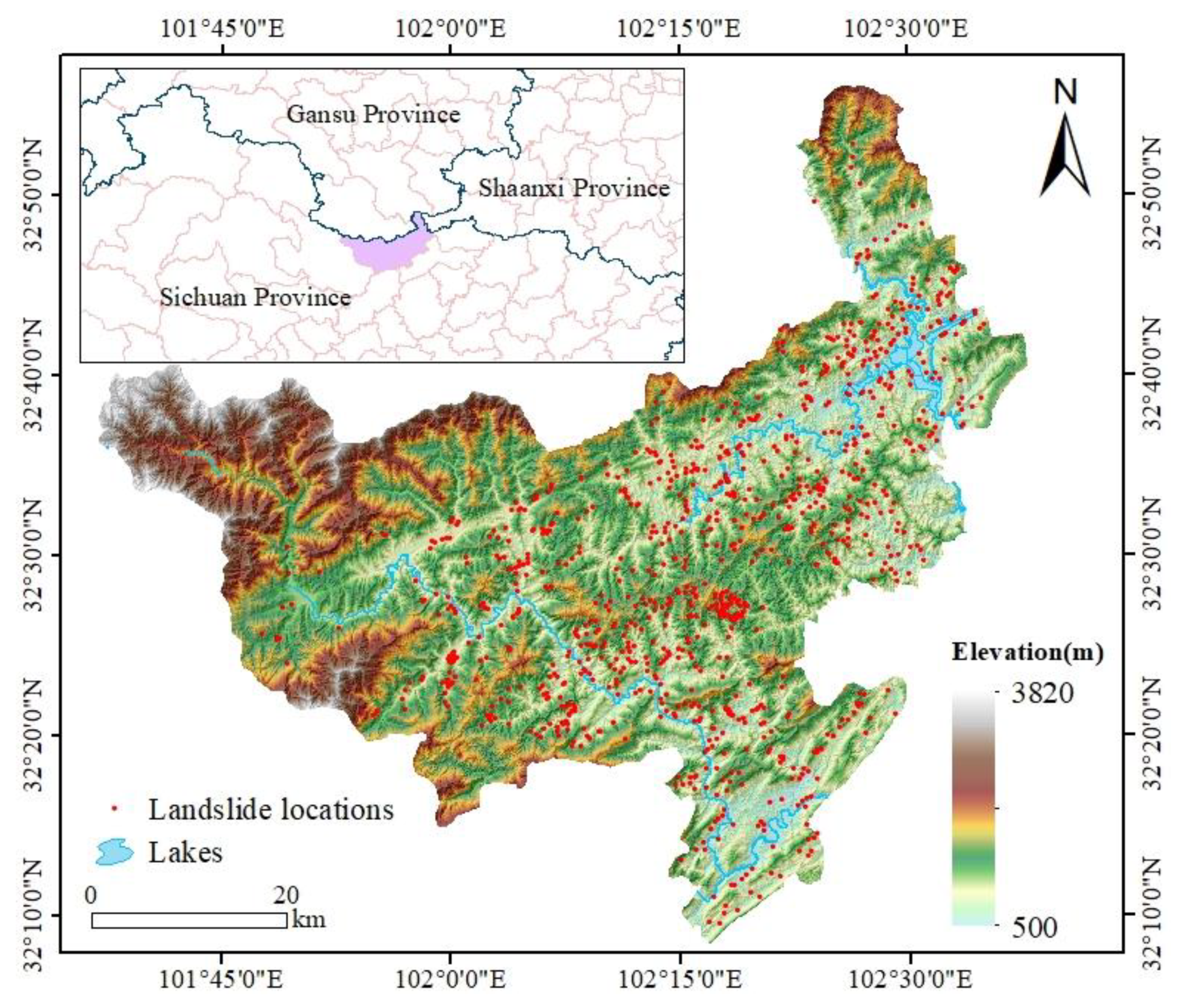
The southeastern area of China is a region with frequently occurring landslide hazards. The study area of Qingchuan County is a mountainous region on the northern edge of the Sichuan basin, in the southeast of China, adjacent to Shanxi province and Gansu province. The area is located at a latitude of 32°12′ N to 32°56′ N and a longitude of 104°36′ E to 105°38′ E, with an area of 3216 km2. It has a complex topography mainly composed of mountains, hills, tablelands, valleys, and small flat dams, and the relative elevation is between 500 m and 3820 m.
The climate in the study area is a typically subtropical humid monsoonal climate that is hot and humid in summer and mild and arid in winter. The surface water system is developed, and the Bailong River and Qingzhu River run through the territory. The total water storage is above 15.7 billion m3, and the water energy reserves are larger than 1 million kW. The soil types are diverse, including yellow loam, yellow-brown loam, dark brown loam, and subalpine meadow soil. The dominant lithology is magmatic rocks, metamorphic rocks, and clastic rocks. Three fault zones are distributed in parallel, from northeast to southwest.
Qingchuan County is recognized as one of the most landslide-prone areas of China [40], and the landslide inventory map in Qingchuan is shown in Figure 1. Most landslide events are induced by natural environmental factors, such as rainfall and earthquakes, while only a few events are induced by human factors. Landslides are pivotal disturbances to the social development and socioeconomic growth of the region. LSM considering the spatial non-stationarity scale effect could significantly prevent the issue.
2.2. Dataset Preparation
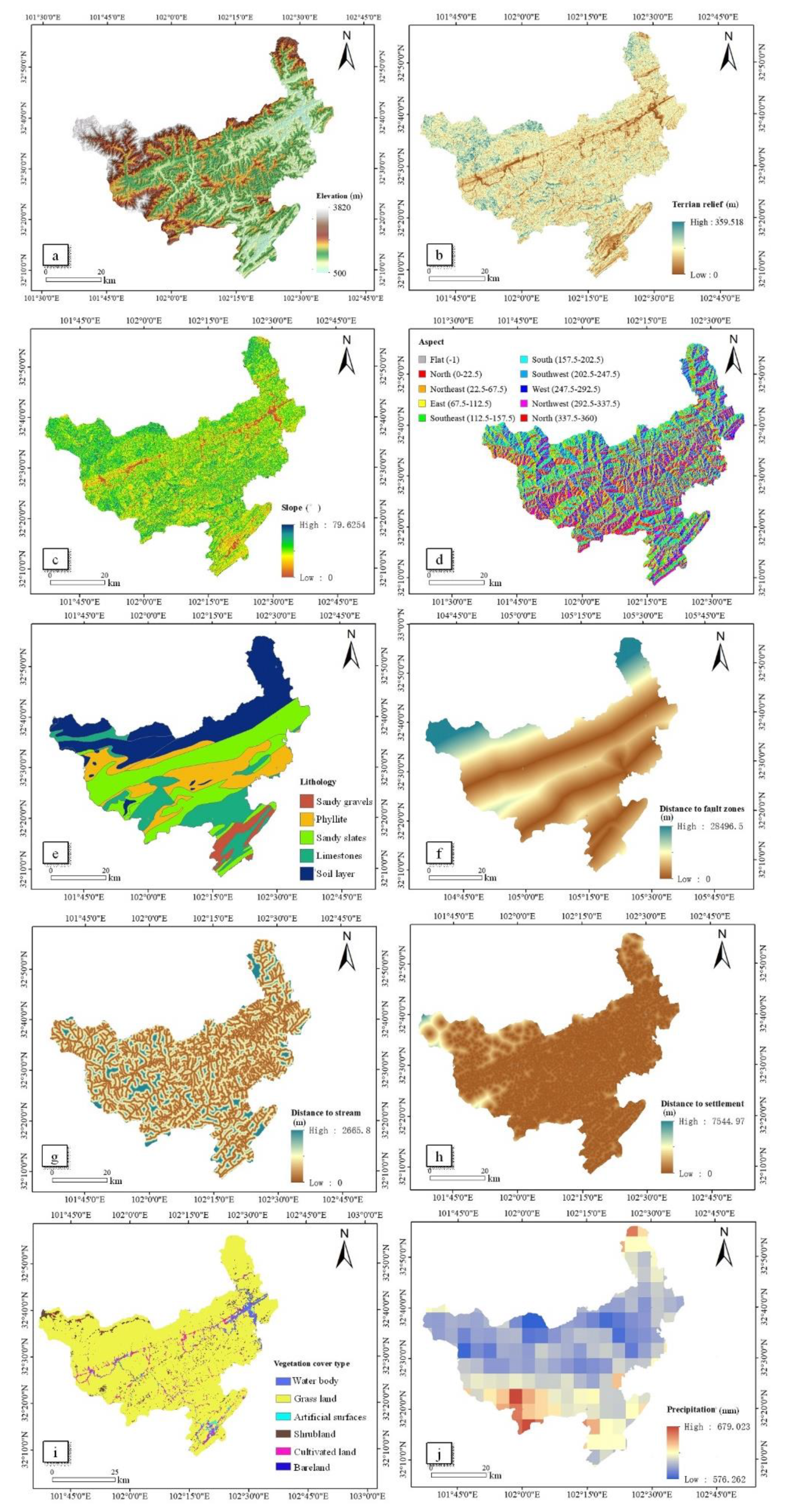
In order to conduct the spatial non-stationarity exploration, the investigation of the spatial dataset was a continuing concern regarding the LSA. The main data included a vector map of contour lines, a geological map, settlement coordinates, aerial photographs, precipitation data, and vegetation coverage types, which were obtained from the Ministry of Land and Resources. After the field survey and aerial photo interpretation, 973 landslides were counted (Figure 1), and the LCFs played an extraordinary role in modeling the LSA [41]. Since there are no standard criteria for selecting LCFs, this study considered the general characteristics, working scale, and availability of the proper datasets [42,43,44]. Ten factors, namely elevation, slope, aspect, terrain relief, lithology, distance to fault zones, distance to stream, precipitation, vegetation coverage types, and distance to settlement, were obtained from GIS (Figure 2).
The digital elevation model (DEM) data at a spatial resolution of 10 m were first obtained by the vector map of contour lines in the GIS environment. The DEM data were used to extract the elevation, slope, aspect, terrain relief, and other conditioning factors describing the topography and geomorphology [45]. Precipitation data and vegetation coverage types were processed through interpolation, collected from different organizations and government departments. Distance to fault zones, distance to stream, and distance to settlement were calculated using a Euclidean distance tool in the GIS environment. In this study, the original data were used as the input of the model for continuous variables, and the unclassified variables were numbered according to their categories before being input into the model.
3. Materials and Methods
3.1. Flowchart
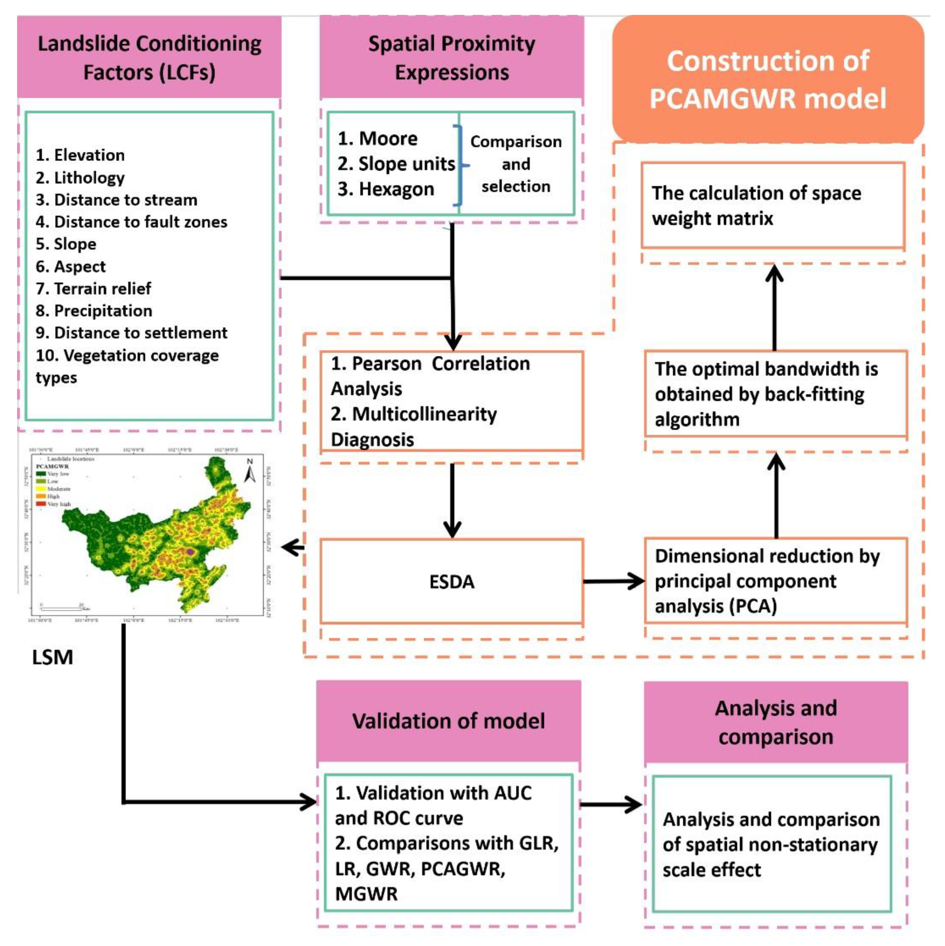
The methodological approach in this study was a methodology combining geospatial statistics and geohazard assessment and is shown in Figure 3. The research process consisted of the following five steps:
- Three spatial neighborhood expressions were constructed in GIS—Moore neighborhoods, slope-unit-based neighborhoods, and hexagonal neighborhoods. The segmentation metric function proposed by Espindola [46] was then used for the prime spatial proximity expression and the extracted LCF was used as the input of the PCAMGWR model.
- Based on the geoenvironmental condition of the study area, LCFs were selected, and thematic layers of LCFs were prepared. Then, the LCFs were analyzed using Pearson correlation analysis and multicollinearity test.
- ESDA was used to investigate the validity of global regression, and the residual obtained by Ordinary Least Squares (OLS) was analyzed based on Moran’s I autocorrelation.
- PCAMGWR model was established for exploring the influence of spatial non-stationarity and factor correlation on LSM.
- The accuracy of the proposed model was verified using statistical measures, and the spatial non-stationarity scale effect was analyzed and compared.
3.2. Expression of Spatial Proximity Selection Method
In this study, three expressions of spatial proximity, namely Moore neighborhoods, slope-unit-based neighborhoods, and hexagonal neighborhoods, were established. The comparison and selection of spatial adjacency expression proceeded in three dimensions, which were homogeneity within a neighborhood, heterogeneity between neighborhoods, and RMSE value of neighborhood area. RMSE values were calculated for the area of the slope-unit-based neighborhoods and hexagonal neighborhoods. The smaller the RMSE value, the more stable the spatial proximity.
Espindola [46] proposed a function to ensure the expression of the spatial proximity of the study area. The function measures the quality of spatial adjacency expression by maximizing homogeneity within and heterogeneity between neighborhoods. The objective function combines the variance measure and the autocorrelation measure:
where is the intersegment variance within the neighborhood and is the Moran’s I to assess the intersegmental heterogeneity between neighborhoods.
3.3. Factor Analysis
3.3.1. Correlation Analysis
Pearson correlation analysis quantifies and interprets the correlation between LCFs [47], and the Pearson correlation coefficient is (−1, 1). If the coefficient is greater than 0, the larger the coefficient is, the stronger the positive correlation. If the coefficient is less than 0, the smaller the coefficient is, the stronger the negative correlation. The Pearson correlation coefficient is defined as follows [48]:
where is the correlation coefficient between two LCFs and is the number of observations.
3.3.2. Multicollinearity Test
Multicollinearity refers to the fact that model estimates are distorted or difficult to estimate accurately due to the existence of accurate or highly correlated relationships between explanatory variables in a linear regression model. Multicollinearity between LCFs may reduce the prediction accuracy of linear regression models, such as GAM-style GWR methods, and the permutation importance of some models, such as (bagged or boosted) tree-based methods, may be faulty. Therefore, the multicollinearity test must be performed before GWR-based model prediction [49]. Variance Inflation Factor (VIF) and TOLerance (TOL) standards were applied for the multicollinearity test [50]. The threshold value of the TOL ≤ 2 and VIF ≥ 5 indicate the existence of multicollinearity between the LCFs [50]. The VIF can be obtained using Equation (3) [51]:
where is the negative correlation coefficient for regression analysis of the ith independent variable to other independent variables.
3.4. ESDA
ESDA denotes whether spatial autocorrelation exists and proves the explicit and quantitative spatial assessment of geographical change [52]. Spatial autocorrelation is a connatural peculiarity of geospatial datasets [53]. However, previous studies have seldom paid attention to the frequent occurrence of spatially autocorrelated residuals in regression models, which indicate a model misspecification problem and unreliable results [54]. To judge whether the global regression result was valid, the residual value of global regression was analyzed by the Moran index. If and , the data are positively aggregated.
3.5. Validation Method
The comprehensive performance of the proposed model in LSA was appraised. Several validation methods were employed for the model fitting degree and accuracy of model prediction, such as the Akaike Information Criterion (AICc). Area Under the ROC Curve (AUC) and the ROC curve were used to assess the accuracy of models [55]. The ROC curve took the false-positive rate specificity as the horizontal coordinate (the proportion of neighborhoods without landslide hazards that were correctly predicted) and the true-positive rate sensitivity as the vertical coordinate (the proportion of neighborhoods with landslide hazards that were correctly predicted). The AUC is the area under the ROC curve, which can more intuitively express the prediction accuracy of models. Its value range is (0.5, 1). The closer the value is to 1, the higher the model accuracy will be. It is generally considered that the prediction accuracy interval (0.5, 0.7) is relatively reasonable, (0.7, 0.8) is reasonable, and (0.8, 1) is very reasonable. If the AUC is extremely close to 1, the model reflects higher goodness-of-fit and consummate accuracy [56].
4. PCAMGWR Modeling
4.1. Principal Component Analysis (PCA)
PCA is an effective method for dimensionality reduction and the feature combination analysis of multivariate factors, which describes multivariate samples to identify spatial patterns [31]. PCA employs an orthogonal transformation to transform correlated variables into linearly unrelated variables, namely independent Principal Components (PCs) [57,58,59]. The first PC had the most significant contribution and contained as much information about the LCFs as possible, followed by the second PC and the third PC. The steps for eliminating factor correlation were as follows: (1) standardized processing of the original LCFs; (2) calculating the correlation coefficient matrix of the standardized matrix; (3) calculating the eigenvalues and eigenvectors of the coefficient matrix to determine the PCs; (4) computing the variance contribution rate and determining the number of PCs; (5) comprehensively evaluating the PCs.
4.2. MGWR
GWR is a linear regression but differs from traditional linear regressions in that GWR considers the influence of spatial relations on the model, namely spatial heterogeneity. GWR is one of the methods used in the exploration of spatial non-stationarity [60], and the regression coefficients change with the spatial location. However, there are limitations to this method, namely that it is useless for spatial multicollinearity [61] and neglects changes in the spatial scope of geographical units [62,63,64]. The MGWR model can solve these issues [65]. Consequently, the PCAMGWR model considering the spatial non-stationarity scale effect based on hexagonal neighborhoods was employed to assess landslide susceptibility.
Assuming that there are observations, for the observation at location with m independent variables, where at the j-th independent variable, the GWR model formulation is described as follows:
where is the j-th independent variable; is the j-th coefficient; is the error term; and is the i-th dependent variable.
The MGWR model is mathematically expressed as follows [34,66]:
where in indicates the bandwidth used for calibration of the j-th spatial relationship. The selection of the bandwidth was relatively ordinary due to a single bandwidth required. By the trial selection of an initial bandwidth, the AICc was optimized to select the bandwidth, which is defined as:
where is the sum of the error terms’ square residual, and is the trace of the hat matrix and the Effective Number of Parameters (ENP) of the model. The bandwidth with the smallest AICc value was optimal. The Gaussian kernel data-borrowing scheme parameterized via AICc optimization was utilized throughout. However, the AICc cannot select bandwidths in MGWR on account of the great number of potential combinations of bandwidths, which may generate a different procedure required.
Model calibration for a Gaussian MGWR can be conducted by resorting to weighted least squares. The coefficient at the location is estimated in Equation (7), where is the design matrix and is the spatial weighting matrix for location . is homogeneous for each relationship, with the identical bandwidth being adopted for all the relationships in the model.
The fixed Gaussian kernel function was used to calculate the spatial weights in MGWR on a par with GWR, which can be written as [48]:
where is the weight value of observation for estimating the coefficient of observation ; is the straight-line distance between observations and ; and is a constant bandwidth.
The back-fitting algorithm was adopted to calibrate the MGWR model, which maximizes the expected log-likelihood and is generally used to calibrate generalized additive models (GAMs) [67]. The logic of GAM, in MGWR is defined as the j-th additive term resulting in the GAM-style MGWR:
The back-fitting algorithm was a smoother method for calibrating the model, and the specific process was as follows [65]. Firstly, all additive terms were initialized, the dependent variables set, and the errors calculated. These errors, plus the “current” value of the first term , were then regressed on using GWR, which produced an optimal bandwidth for the relationship between and , as well as a new set of local estimates for the relationship between and that was used to update the value of the first term . The second variable followed the same procedure as above, and the process was repeated until the first iteration was completed. The iteration continued until the change of all terms in successive iterations was less than the score of change (SOC).
Two decisions from the user are involved in the algorithm. The first concern is initializing the local coefficient estimates, which might affect the number of iterations needed to reach convergence instead of the selection of the optimal bandwidth. The GWR was thus used to estimate the initial MGWR. The second decision is the choice of the termination criterion—the value of the differential between successive iterations, namely the SOC by which the process is converged. SOC-f focuses on the relative changes of the additive terms rather than on overall model fitting. The calculation formula of SOC-f is as follows:
5. Results
5.1. Expression of Spatial Proximity
The spatial proximity of the study region was expressed in the GIS environment, which incorporated Moore neighborhoods (Figure 4a), slope-unit-based neighborhoods (Figure 4b), and hexagonal neighborhoods (Figure 4c).
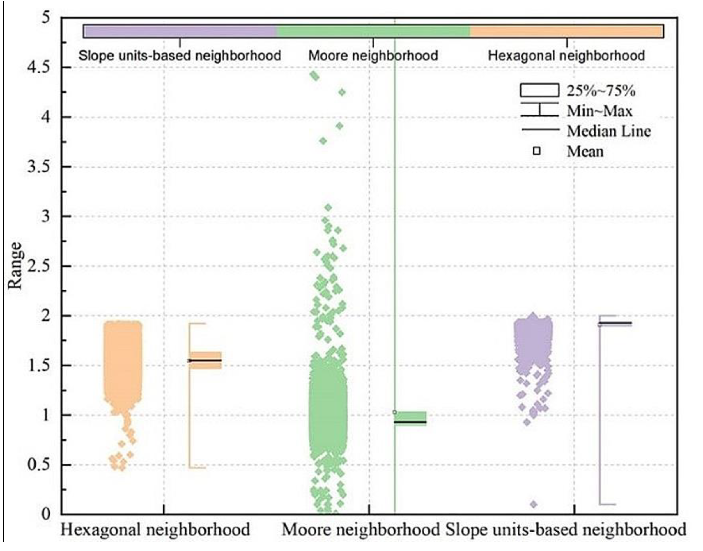
The present research primarily explored the homogeneity within the neighborhood and the heterogeneity between the neighborhoods, as shown in Figure 5. The hexagonal neighborhoods are shown in orange, the Moore neighborhoods in green, and the slope-unit-based neighborhoods in purple. The solid lattice of diamonds on the left represents the distribution of the F values in each type of neighborhood. On the right is a box plot to figure out the distribution characteristics of the F value. The black horizontal line is the middle line of the F value, and the box represents the range of 1/4 to 3/4. The F value ranges of the hexagonal neighborhoods, Moore neighborhoods, and slope-unit-based neighborhoods were, respectively, (0.47, 1.92), (0, 5), and (0.1, 2). The F value distribution in the hexagonal neighborhoods was relatively concentrated and the spectrum was small. The medians were ordered as follows: slope-unit-based neighborhoods, hexagonal neighborhoods, Moore neighborhoods. From the distribution of the F value, slope units and hexagons performed better. To further select the most suitable expression of spatial proximity, the RMSE values of the slope elements and hexagons were calculated, and the hexagonal neighborhoods expressed the spatial proximity of the study area with a greater RMSE.
5.2. Correlation Analysis and Multicollinearity Test
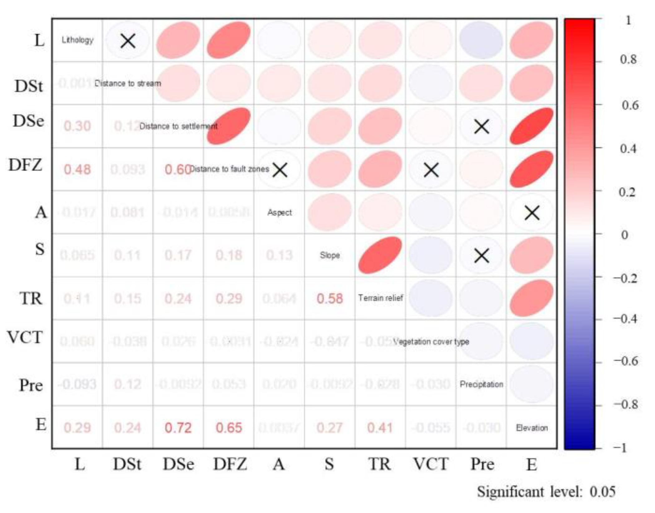
Pearson correlation analysis of the LCFs was conducted as a preliminary analysis, as shown in Figure 6. The darker the red is, the stronger the positive correlation; the darker the blue is, the stronger the negative correlation. The maximum correlation coefficient was 0.72 for the distance to settlement and elevation, revealing that the higher the elevation is, the fewer the settlements. The correlation coefficients between the distance to the fault zones and distance to settlement, the terrain relief and slope, the elevation and distance to the settlement, and the elevation and distance to fault zones were between 0.5 and 0.8, showing a moderate positive correlation. The other factors were weakly correlated or irrelevant. The symbol × in Figure 6 indicates no statistically significant correlation between factors. There were no highly correlated factors among the LCFs selected in this study.
Regression analysis is prone to producing high multicollinearity between independent variables. To test the global multicollinearity, the VIFs of various LCFs were calculated, as shown in Table 1. A VIF value greater than 10 denotes the existence of global multicollinearity. In this study, the maximum VIF value was 2.861, lower than 5, indicating that all LCFs passed the global multicollinearity test.
5.3. ESDA
ESDA is an essential method that was used to examine the spatial associations among the LCFs and aid with the model development. A classic spatial autocorrelation index, namely the Moran’s I, was computed using the residual of global regression and was implemented to explore the spatial non-stationarity effects [68].
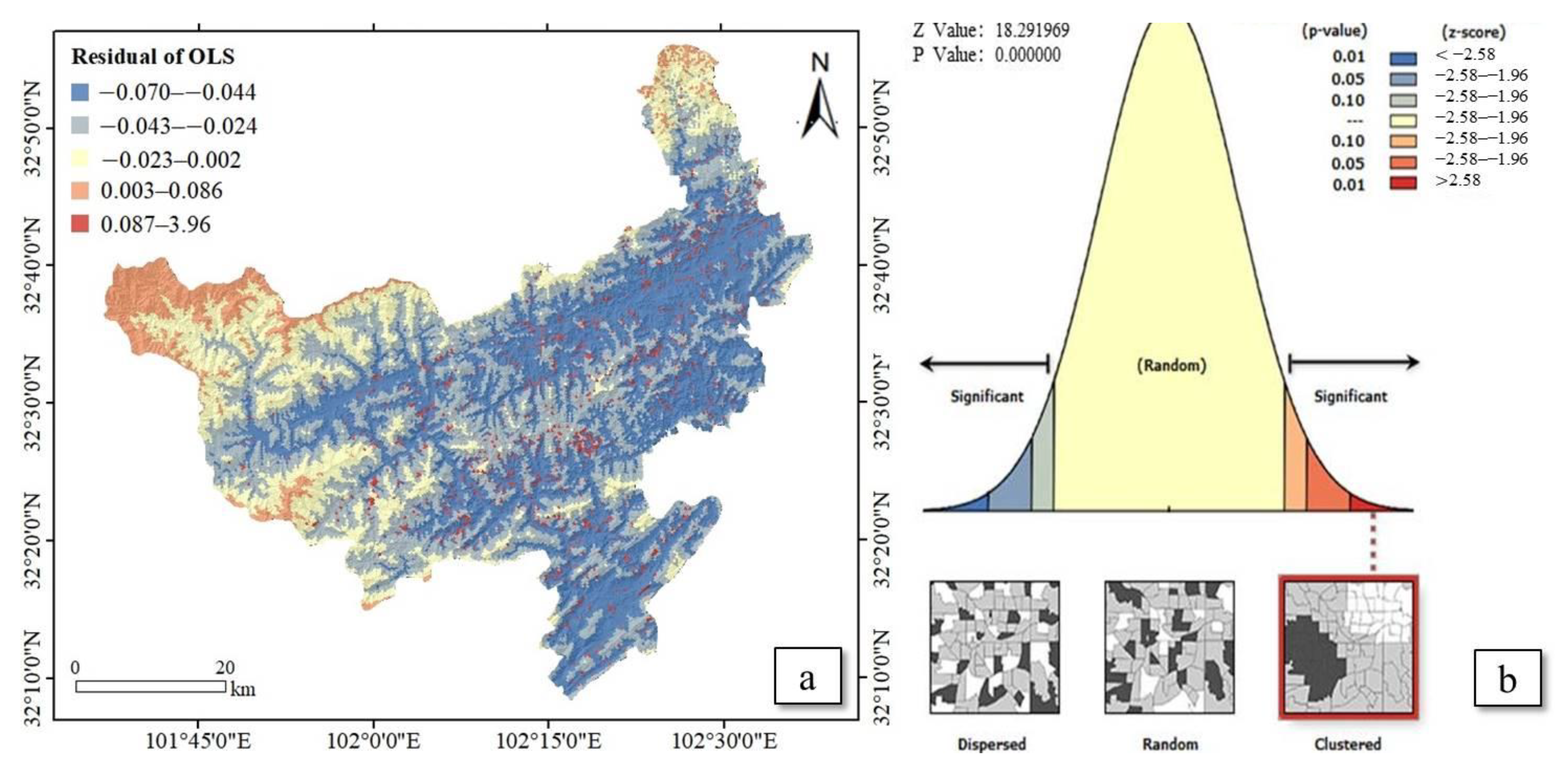
The landslide susceptibility prediction based on OLS was carried out, and the residual distribution is shown in Figure 7a. The red area is highly consistent with the location of the landslides. The Moran’s index analysis based on OLS residual values judges the effectiveness of global regression results. If and , it is a positive aggregation. The Moran’s index analysis gave a result of and the Z value was 18.292, indicating that the global regression was invalid. The residual was spatially autocorrelated to a level of statistical significance, which was brought about by a non-stationary spatial process (Figure 7b). Therefore, a model with an interpretation of spatial non-stationarity relationships is necessary for LSA.
5.4. LSMs Based on PCAMGWR Model
Six principal components were obtained by principal component analysis and are shown in Table 2. The overall contribution rate was 82.704% to represent the entirety elementarily. PC1 was interpreted as a comprehensive factor, since it has a high favorable loading of elevation, distance to fault zones, distance to settlement, and terrain relief. PC2 has a high favorable loading of the slope. PC3 has a high positive loading of precipitation. PC4 has high favorable loading of vegetation cover type. PC5 has a high negative loading of aspect. PC5 has a high negative loading of distance to stream.
Normal distribution and axle-whiskers were employed to analyze the differences between the PCs and LCFs, respectively, as shown in Figure 8. Although the original LCFs obeyed normal distribution, there was a significant difference between the factors, and the data were more discrete. The distribution of the principal components was more uniform and closer to the standard normal distribution using the principal component analysis.
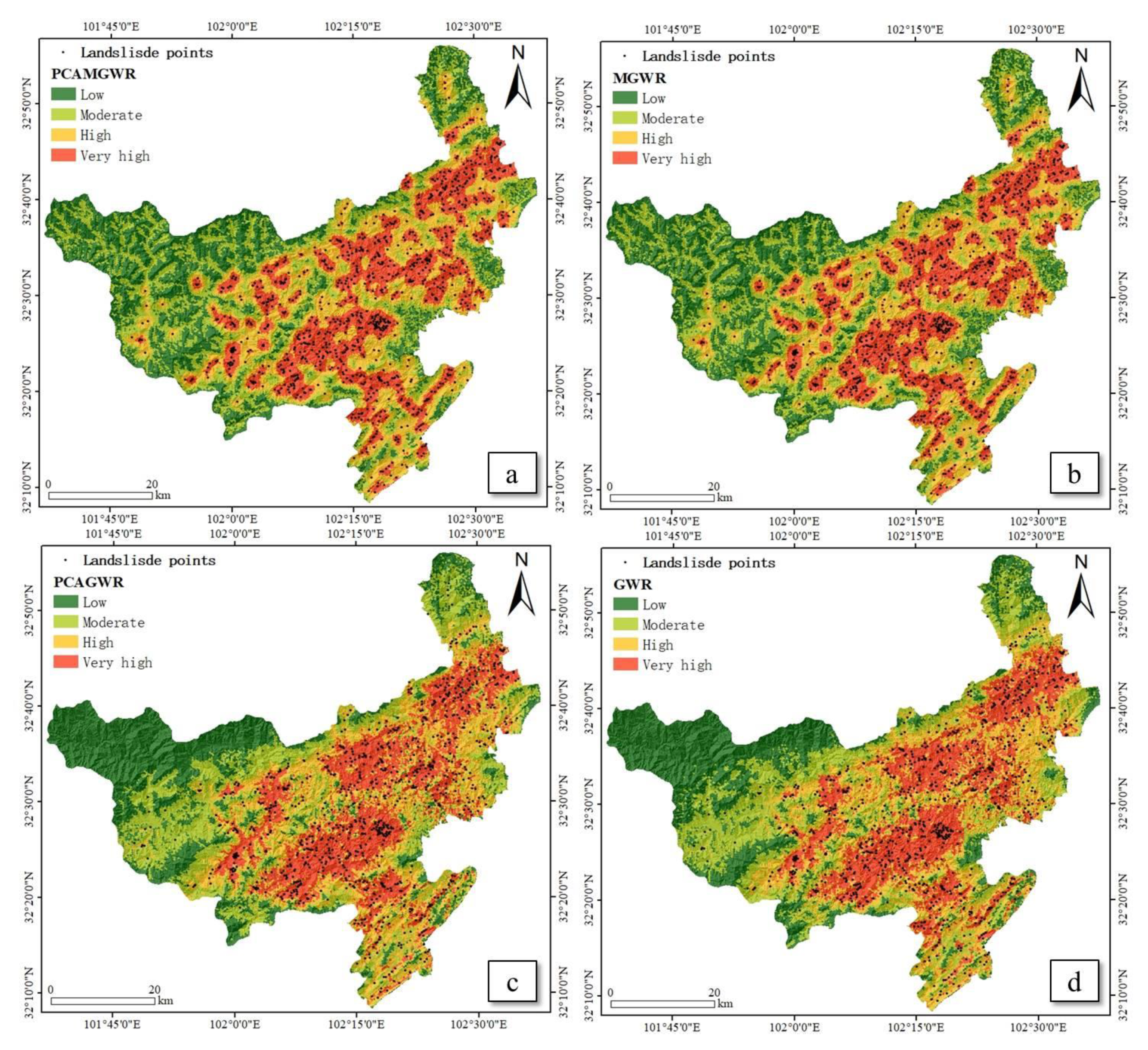
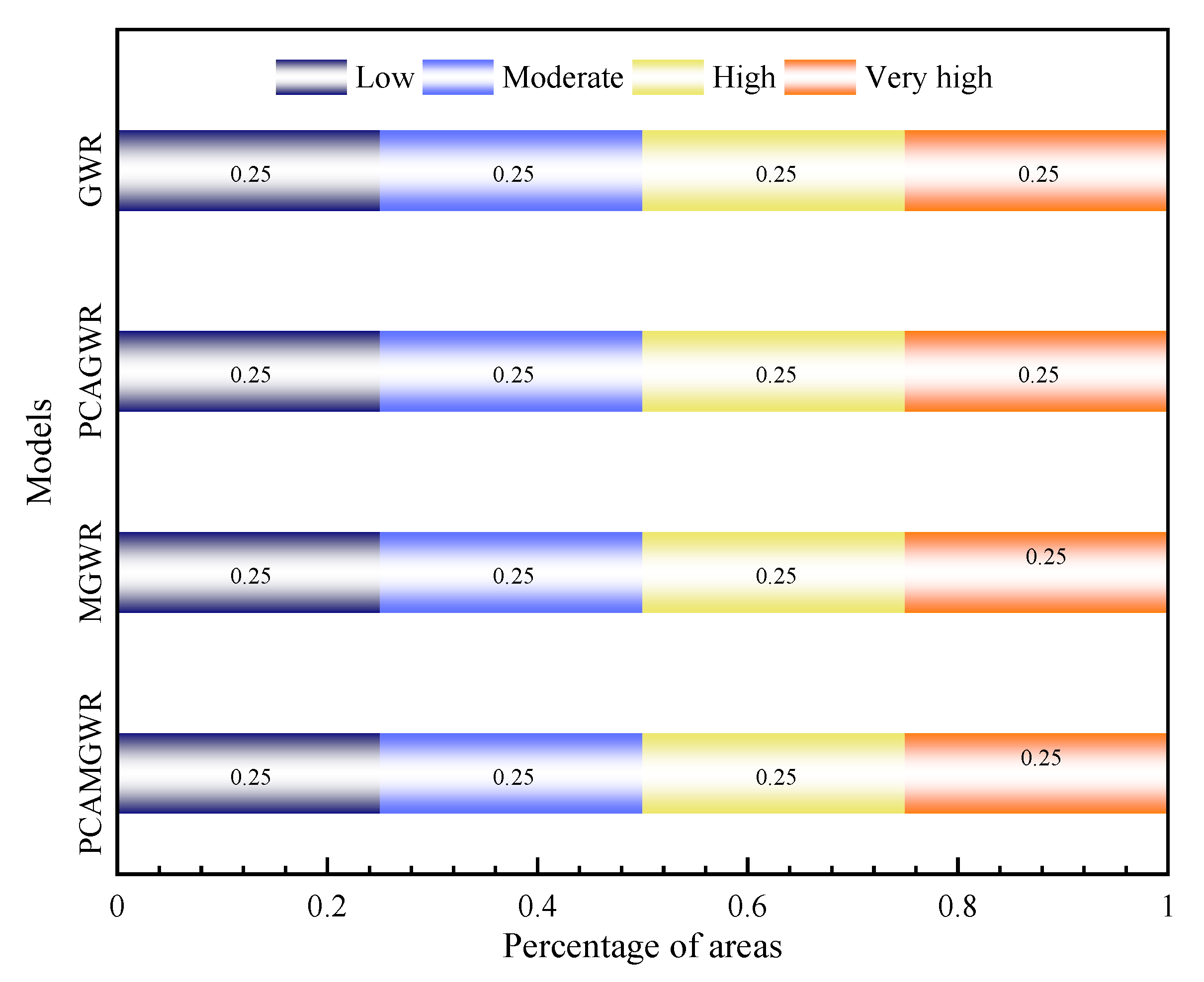
The LSMs of the study area were independently obtained using the PCAMGWR, MGWR, PCAGWR, and GWR models, as show in Figure 9. The LSMs were divided into four levels using the quantile method, namely low, moderate, high, and very high susceptibility. Figure 10 shows the area percentage of very high, high, moderate, and low susceptibility.
The PCAMGWR and MGWR models exhibited more veracious and reasonable predictions. The high and very high susceptibility areas were more consistent with investigated landslide locations due to the consideration of the scale difference effect of spatial non-stationarity. Apart from the significant variances in the land area composition with the various landslide susceptibility levels, the landslide susceptibility zoning results of the two models considering the spatial non-stationarity scale differences were better combined with topographic factors. The PCAMGWR and MGWR models comprehensively considered topography, streams, and settlements. Especially in the western mountainous area, the landslide susceptibility was low in the area with very high altitude but far from the river and with rare human activities, while the landslide susceptibility was medium in the area with high altitude and close to the river and human activities. It can be seen that the PCAMGWR model proposed in this study can reflect the non-stationarity scale difference in the spatial relationship between LCFs and landslides. Moreover, the LSMs based on the PCAMGWR model and MGWR model were similar, indicating that MGWR can deal with factor correlation and multicollinearity. There was a large gap between the LSMs based on the MGWR-based models and GWR-based models, which can be seen considering the spatial non-stationarity scale difference, making the zoning results tend towards the actual situation. In addition, there were many similarities between the four models. There were southwest–northeast spatial distributions along fault zones in the LSMs obtained using the four models, which may be attributed to the fault zones’ influences on slope and rock mass stability.
5.5. Analysis and Comparison of Spatial Non-Stationarity Scale Effect
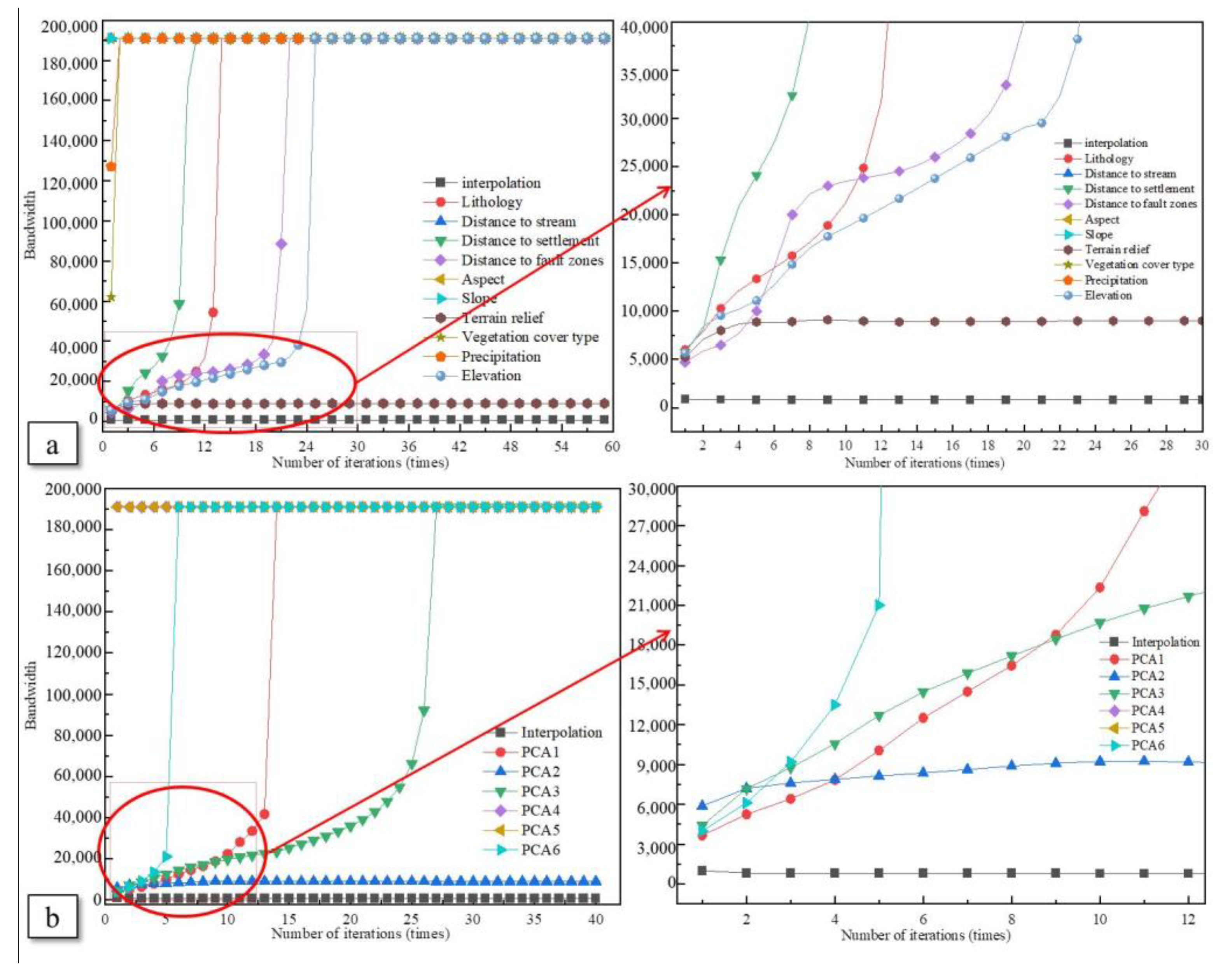
Compared with the GWR model, the MGWR model showed an improvement in the research of spatial non-stationarity. MGWR allowed the parameter estimates to vary spatially and generated a single optimal scale (bandwidth) for the non-stationary spatial relationship between landslides and each independent variable. The spatial variation of different processes was modeled at different spatial scales. The optimal bandwidths deduced by the GWR, PCAGWR, MGWR, and PCAMGWR models were direct indicators of spatial scale, indicating the individual spatial relationship between landslide and independent variables. Figure 11 indicates the bandwidth search process for each independent variable generated by the MGWR model (Figure 11a) and PCAMGWR model (Figure 11b), a process that was observed to operate at different spatial scales.
A variable with a large bandwidth affects the dependent variable at a large scale, so the standard deviation of the parameter estimates is slight. In contrast, a variable with a small bandwidth affects the dependent variable at a local scale, so the standard deviation of the local parameter estimates is significant. The optimal bandwidth of terrain relief and interpolation was 9018.89 and 784.84 in the MGWR model, with the number of iterations being 59. Additionally, the variable affected landslide susceptibility at the local scale, and its parameter estimate had significant variances over space. The relationships between the other nine LCFs and landslides exhibited spatial non-stationarity, but the processes varied at regional spatial scales. In the PCAMGWR model, PC2 and interpolation demonstrated solid locally spatial non-stationarity scale effects, and the optimal bandwidth was 8962.5 and 784.32. The number of iterations of the PCAMGWR model was 40. The spatial non-stationarity scale effects between the other principal components and landslides were at the regional scale. Bandwidth selection for different parameters may stop at different steps depending on the properties of the spatial non-stationarity scale effect.
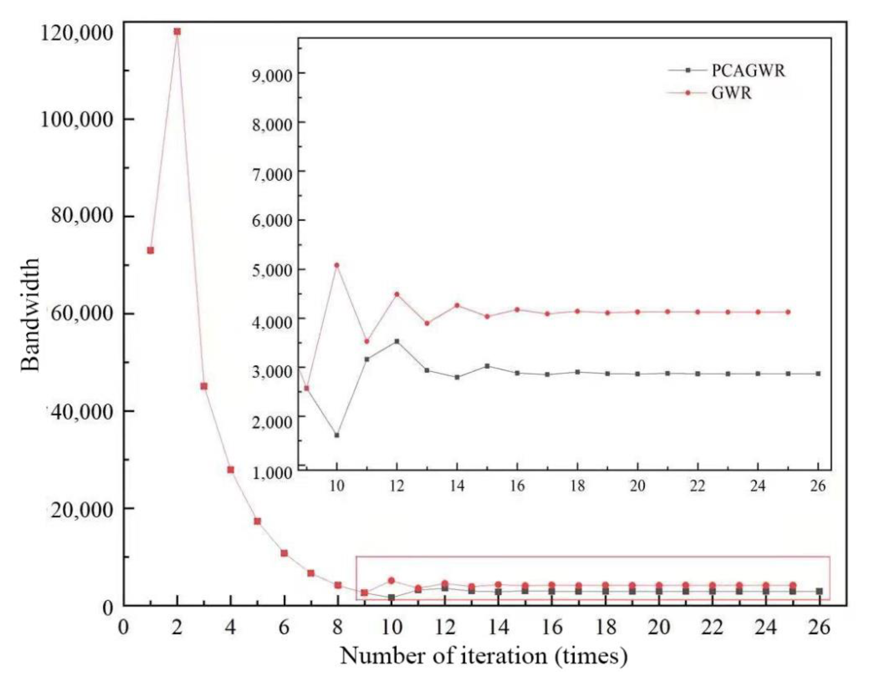
However, the optimal bandwidths generated using the GWR model and PCAGWR model were 4127.02 and 2868.55, which implies that all variables affected landslides with the same spatial non-stationarity scale effect of extreme restriction. The bandwidth produced by GWR or PCAGWR was the weighted average of the independent spatial processes of each factor and landslides, with varying degrees of spatial non-stationarity, as shown in Figure 12. The convergence rate of the two models was similar under the same scale effect, and there was no continuous decline in AICc values. The weighting is a function of the explanatory ability of each relationship in the local model.
5.6. Validation and Accuracy Assessment
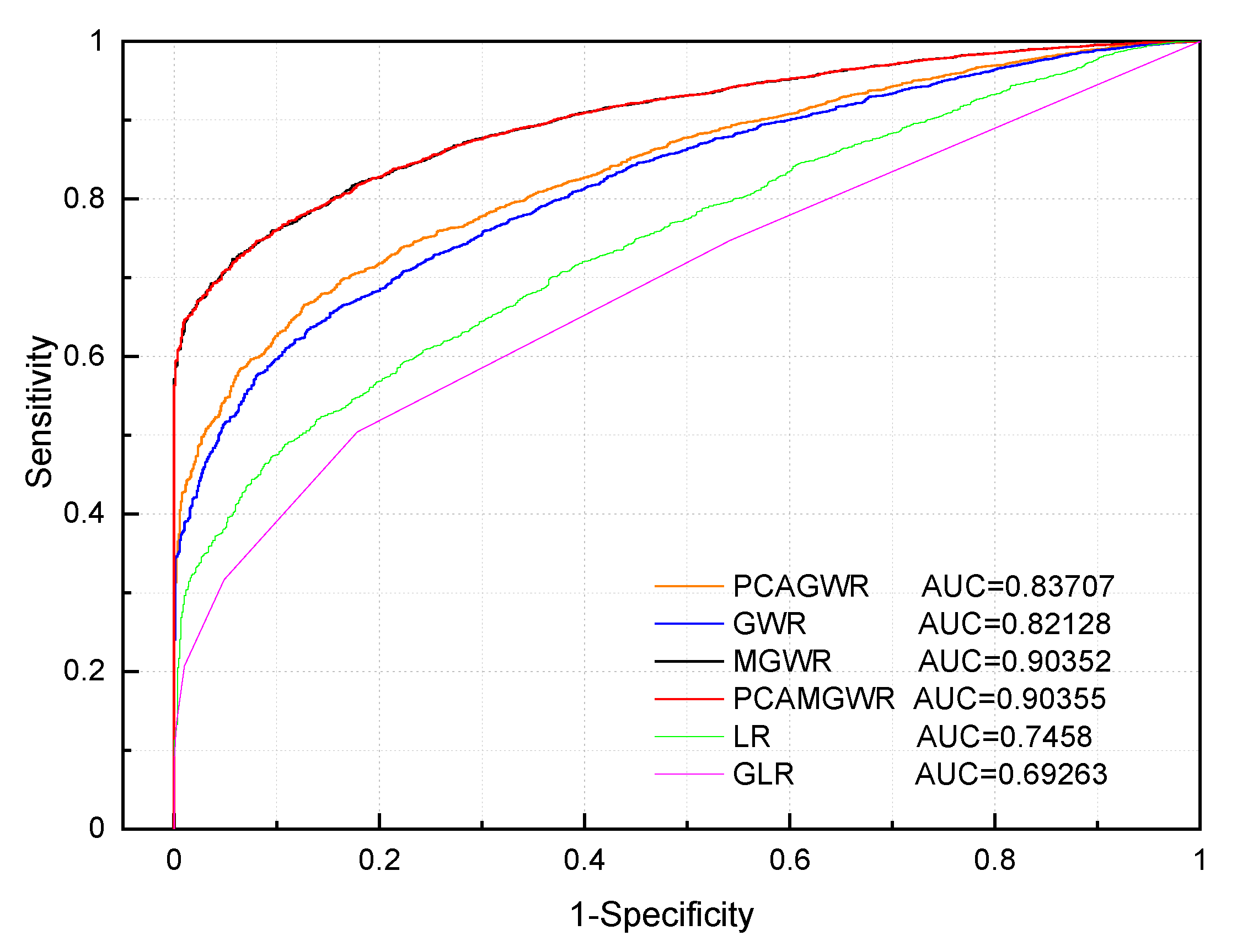
The whole dataset was input into the ROC calculation tool of origin software to obtain the ROC curve and AUC value. The accuracy of the model prediction was validated by the AUC and other statistical indicators, shown in Table 3. The bandwidth selection criterion of the basic GWR model was the minimum AICc value, and the bandwidth selection criterion of the MGWR and PCAMGWR models was SOC-f dissimilarity, but the AICc value could still be enumerated. Therefore, The AICc value served as a valid indicator of the model prediction. The PCAMGWR model had the minimum AICc value of 78,291.042 and indicated the maximum accuracy of bandwidth selection and model prediction, with the AIC value also being the minimum, while the BIC value was inferior to GWR. The ROC curves of various models are drawn in Figure 13, and the AUCs of Global Linear Regression (GLR), Logistic Regression (LR), GWR, PCAGWR, MGWR, and PCAMGWR were, respectively, 0.69263, 0.7458, 0.82128, 0.83707, 0.90352, and 0.90355. The MGWR model considering multiscale bandwidth showed a significant improvement in the accuracy of prediction results compared with the GWR model. Consequently, spatial non-stationarity scale variances were subsistent between LCFs in the study area, and it is significant to identify spatial non-stationarity scale effects in LSA.
Meanwhile, the assessment results of the PCAGWR compared with GWR provided a significant priority ranking. The assessment results of the PCAGWR model were more accurate than those of GWR regarding the elimination of local collinearity. The AUC of PCAMGWR increased less than that of MGWR, and the PCA had a minor role in collinearity elimination for the PCAMGWR model, which is reflective of the fact that the MGWR model could eliminate most of the local collinearity of LCFs to improve the prediction accuracy of landslide susceptibility.
6. Discussion
Landslides are a major geohazard, causing casualties and economic losses. Therefore, it is necessary to establish a suitable model to assess landslide susceptibility and make a landslide zoning map. The assessment methods and models of landslide susceptibility have been discussed in many studies. For example, a comparative study of WOE, AHP, ANN, and GLR procedures for landslide susceptibility zonation is presented in [69]. WOE can assess the impact of different classes of each LCF, but neglects the correlation between LCFs. The logistic regression (LR) method is a static susceptibility model that has limited application for predicting future landslide probability under potential rainfall events [70]. Moreover, LR is capable of analyzing the relationship among the LCFs, but it is not able to evaluate the impact of different classes [71]. A support vector machine (SVM) is a machine learning algorithm that uses a small number of samples, but a high-quality informative database is essential to improve model performance [72].
Compared with the assessment method of LSA, the study of the essential attribute, namely the spatial non-stationarity, of the landslide as a geospatial phenomenon is insufficient. At present, a small number of scholars have carried out studies on the consideration of spatial non-stationarity and the application of the GWR idea in LSA, and have proved that the GWR model is superior to some traditional models, such as global linear regression (GLR) [21,33], ANN and OLS [73], SVM [74], and SR [30]. However, there is a research gap in the study of the non-stationarity scale of the spatial relationship between landslides and LCFs.
This study mainly discusses the influence of spatial non-stationarity on LSA results and the difference of spatial non-stationarity scale among different factor combinations. In addition, spatiotemporal non-stationarity is rarely considered in the study of geospatial data, especially in the field of geological hazard assessment. In this study, only spatial non-stationarity was considered. Therefore, time may be introduced into non-stationarity in geospatial data studies. The analysis of the impact of scale variance on model prediction accuracy is a main area of focus. The impact of such variance is more directly reflected in the spatial differentiation of regression coefficients, which is a shortcoming in the present study. In addition, the studies regarding GWR and MGWR models take full datasets as the model input without considering the division of training set and testing set [21,75,76]. The indicators which are generated during the model run, such as AICc, are generally used for model performance testing, and the present study also verified the assessment accuracy using these indicators. However, most LSA studies divide the training set and testing sets, and future studies can thus focus on the comparison between analysis with and without division methods. On the other hand, the present study analyzed the spatial non-stationarity scale of landslide susceptibility using GAM-style MGWR. Thus, future studies can explore the interaction effects and nonlinear relationships. Moreover, the LSMs were related to zoning methods, and the quantile method was selected for the zoning of the landslide susceptibility map, which may have reduced the accuracy. All data used for model input were normalized, and the influence of the normalization process on a non-stationarity scale is uncertain, which affects the explanatory power of the model. The degree of elimination of local collinearity by the MGWR model may have been related to the composition of LCFs, which needs to be further studied. These limitations may further give rise to uncertainties in LSA.
7. Conclusions
Geospatial data may lead to the spatial non-stationarity process, and the scale at which each independent variable affects a dependent variable may vary according to the independent variables. The present study thus considered spatial non-stationarity and scale variations in LSA using a PCAMGWR model. The results indicated that the PCAMGWR model provides more reliable information for LSA than other GWR models and achieves a higher accuracy in LSM by performing better at alleviating residual autocorrelation.
The present study determined the respective bandwidths for each independent variable and revealed the association between the independent variables and landslide susceptibility using the PCAMGWR model. The model relaxes the single-bandwidth assumption of the basic GWR model and allows independent variable-specific bandwidths to be optimized. The results demonstrated that there are scale variations in LSA. For example, PC2 affected the landslide susceptibility at a local scale, namely the local parameters associated with the variable varied across space. The basic GWR model was outperformed at differentiating such scale variations and can be substituted by PCAMGWR.
Moreover, according to the AUCs, compared to GLR and LR, the PCAMGWR and MGWR models can better analyze the impacts of non-stationarity scale variation and factor correlation on LSM than GWR and PCAGWR. The four models with and without the elimination of factor correlations were compared, and it was indicated that the PCAGWR and PCAMGWR models benefited from the elimination of factor correlations by PCA, and the PCAMGWR model was preferred to PCAGWR because the scale variation of spatial non-stationarity had a greater impact than factor correlation. Meanwhile, the MGWR and PCAMGWR models benefited from the consideration of the scale variation, and PCAMGWR was preferred to MGWR. Spatial statistical models are useful for analyzing the determinants of landslide susceptibility by considering spatial dependency and spatial heterogeneity. The present study reveals the superiority of a new approach, namely the PCAMGWR model, to consider the spatial characteristics, non-stationarity scale variations, and factor correlations.
Author Contributions
Y.L. led the research program; S.H. and Y.L. designed the algorithm; S.H. wrote the manuscript; J.L., W.W. and J.H. reviewed and edited the manuscript. All authors have read and agreed to the published version of the manuscript.
Funding
This study was founded by the National Key Research and Development Program of China (grant number 2018YFD1100401); the National Natural Science Foundation of China (grant number 52078493); the Natural Science Foundation for Outstanding Youth of Hunan Province (grant number 2021JJ20057); and the Innovation Province Program of Hunan Province (grant number 2020RC3002).
Institutional Review Board Statement
Not applicable.
Informed Consent Statement
Not applicable.
Data Availability Statement
The data used in this study are available on request from the corresponding author.
Acknowledgments
Financial support is gratefully acknowledged.
Conflicts of Interest
The authors declare no conflict of interest.
References
- Froude, M.J.; Petley, D.N. Global fatal landslide occurrence from 2004 to 2016. Nat. Hazards Earth Syst. Sci. 2018, 18, 2161–2181. [Google Scholar] [CrossRef] [Green Version]
- Haque, U.; da Silva, P.F.; Devoli, G.; Pilz, J.; Zhao, B.; Khaloua, A.; Wilopo, W.; Andersen, P.; Lu, P.; Lee, J.; et al. The human cost of global warming: Deadly landslides and their triggers (1995–2014). Sci. Total Environ. 2019, 682, 673–684. [Google Scholar] [CrossRef] [PubMed]
- Available online: http://www.mnr.gov.cn/ (accessed on 1 June 2021).
- Guzzetti, F.; Reichenbach, P.; Cardinali, M.; Galli, M.; Ardizzone, F. Probabilistic landslide hazard assessment at the basin scale. Geomorphology 2005, 72, 272–299. [Google Scholar] [CrossRef]
- Corominas, J.; Esgleas, J.; Baeza, C. Risk mapping in the Pyrenees area: A case study. Hydrol. Mt. Reg. II Artificial Reserv. Water Slopes 1990, 194, 425–428. [Google Scholar]
- Zhu, A.X.; Wang, R.; Qiao, J.; Chen, Y.; Cai, Q.; Zhou, C. Mapping landslide susceptibility in the Three Gorges area, China using GIS, expert knowledge and fuzzy logic. In Proceedings of the International Conference of GIS Remote Sensing in Hydrology, Water Resources and Environment, Sandouping, China, 16–19 September 2004; pp. 385–391. [Google Scholar]
- Sarkar, S.; Kanungo, D.P.; Patra, A.K.; Kumar, P. GiS based spatial data analysis for landslide susceptibility mapping. J. Mt. Sci. 2008, 5, 52–62. [Google Scholar] [CrossRef]
- Magliulo, P.; Di Lisio, A.; Russo, F. Comparison of GIS-based methodologies for the landslide susceptibility assessment. Geoinformatica 2009, 13, 253–265. [Google Scholar] [CrossRef]
- Feizizadeh, B.; Blaschke, T.; Ieee. Comparing Gis-Multicriteria Decision Analysis for Landslide Susceptibility Mapping for the Urmia Lake Basin, Iran. In Proceedings of the IEEE International Geoscience and Remote Sensing Symposium (IGARSS), Munich, Germany, 22–27 July 2012; pp. 5390–5393. [Google Scholar]
- Panchal, S.; Shrivastava, A.K. Application of analytic hierarchy process in landslide susceptibility mapping at regional scale in GIS environment. J. Stat. Manag. Syst. 2020, 23, 199–206. [Google Scholar] [CrossRef]
- Ayalew, L.; Yamagishi, H.; Marui, H.; Kanno, T. Landslides in Sado Island of Japan: Part II. GIS-based susceptibility mapping with comparisons of results from two methods and verifications. Eng. Geol. 2005, 81, 432–445. [Google Scholar] [CrossRef]
- Wang, W.D.; Xie, C.M.; Du, X.G. Landslides susceptibility mapping based on geographical information system, GuiZhou, south-west China. Environ. Geol. 2009, 58, 33–43. [Google Scholar] [CrossRef]
- Chalkias, C.; Kalogirou, S.; Ferentinou, M. Landslide susceptibility, Peloponnese Peninsula in South Greece. J. Maps 2014, 10, 211–222. [Google Scholar] [CrossRef]
- Thiebes, B.; Bell, R.; Glade, T. Deterministic Landslide Susceptibility Analyis-A Case Study in the Swabian Alb. In Proceedings of the Conference -Geomorphology for the Future, Obergurgl, Austria, 2–7 September 2007; pp. 177–184. [Google Scholar]
- Ferentinou, M.; Chalkias, C. Mapping Mass Movement Susceptibility across Greece with GIS, ANN and Statistical Methods; Springer: Berlin/Heidelberg, Germany, 2013. [Google Scholar]
- Zezere, J.L.; Pereira, S.; Melo, R.; Oliveira, S.C.; Garcia, R.A.C. Mapping landslide susceptibility using data-driven methods. Sci. Total Environ. 2017, 589, 250–267. [Google Scholar] [CrossRef] [PubMed]
- Chauhan, S.; Sharma, M.; Arora, M.K.; Gupta, N.K. Landslide Susceptibility Zonation through ratings derived from Artificial Neural Network. Int. J. Appl. Earth Obs. Geoinf. 2010, 12, 340–350. [Google Scholar] [CrossRef]
- Bai, S.B.; Wang, J.; Thiebes, B.; Cheng, C.; Chang, Z.Y. Susceptibility assessments of the Wenchuan earthquake-triggered landslides in Longnan using logistic regression. Environ. Earth Sci. 2014, 71, 731–743. [Google Scholar] [CrossRef]
- Kavzoglu, T.; Sahin, E.K.; Colkesen, I. Landslide susceptibility mapping using GIS-based multi-criteria decision analysis, support vector machines, and logistic regression. Landslides 2014, 11, 425–439. [Google Scholar] [CrossRef]
- Dagdelenler, G.; Nefeslioglu, H.A.; Gokceoglu, C. Modification of seed cell sampling strategy for landslide susceptibility mapping: An application from the Eastern part of the Gallipoli Peninsula (Canakkale, Turkey). Bull. Eng. Geol. Environ. 2016, 75, 575–590. [Google Scholar] [CrossRef]
- Chalkias, C.; Polykretis, C.; Karymbalis, E.; Soldati, M.; Ghinoi, A.; Ferentinou, M. Exploring spatial non-stationarity in the relationships between landslide susceptibility and conditioning factors: A local modeling approach using geographically weighted regression. Bull. Eng. Geol. Environ. 2020, 79, 2799–2814. [Google Scholar] [CrossRef]
- Brenning, A. Spatial prediction models for landslide hazards: Review, comparison and evaluation. Nat. Hazards Earth Syst. Sci. 2005, 5, 853–862. [Google Scholar] [CrossRef]
- O’Sullivan, D. Geographically weighted regression: The analysis of spatially varying relationships. Geogr. Anal. 2003, 35, 272–275. [Google Scholar] [CrossRef]
- Li, J.; Wang, W.; Han, Z.; Li, Y.; Chen, G. Exploring the Impact of Multitemporal DEM Data on the Susceptibility Mapping of Landslides. Appl. Sci. 2020, 10, 2518. [Google Scholar] [CrossRef] [Green Version]
- Leyk, S.; Norlund, P.U.; Nuckols, J.R. Robust assessment of spatial non-stationarity in model associations related to pediatric mortality due to diarrheal disease in Brazil. Spat. Spatio-Temporal Epidemiol. 2012, 3, 95–105. [Google Scholar] [CrossRef] [Green Version]
- Tu, J. Spatially varying relationships between land use and water quality across an urbanization gradient explored by geographically weighted regression. Appl. Geogr. 2011, 31, 376–392. [Google Scholar] [CrossRef]
- Yang, Y.; Liu, J.; Xu, S.; Zhao, Y. An Extended Semi-Supervised Regression Approach with Co-Training and Geographical Weighted Regression: A Case Study of Housing Prices in Beijing. Isprs Int. J. Geo-Inf. 2016, 5, 4. [Google Scholar] [CrossRef] [Green Version]
- Monjaras-Vega, N.A.; Briones-Herrera, C.I.; Vega-Nieva, D.J.; Calleros-Flores, E.; Corral-Rivas, J.J.; Lopez-Serrano, P.M.; Pompa-Garcia, M.; Rodriguez-Trejo, D.A.; Carrillo-Parra, A.; Gonzalez-Caban, A.; et al. Predicting forest fire kernel density at multiple scales with geographically weighted regression in Mexico. Sci. Total Environ. 2020, 718, 137313. [Google Scholar] [CrossRef] [PubMed]
- Liu, K.; Qiao, Y.; Shi, T.; Zhou, Q. Study on coupling coordination and spatiotemporal heterogeneity between economic development and ecological environment of cities along the Yellow River Basin. Environ. Sci. Pollut. Res. 2021, 28, 6898–6912. [Google Scholar] [CrossRef]
- Erener, A.; Düzgün, H.S.B. Improvement of statistical landslide susceptibility mapping by using spatial and global regression methods in the case of More and Romsdal (Norway). Landslides 2010, 7, 55–68. [Google Scholar] [CrossRef]
- Sabokbar, H.F.; Roodposhti, M.S.; Tazik, E. Landslide susceptibility mapping using geographically-weighted principal component analysis. Geomorphology 2014, 226, 15–24. [Google Scholar] [CrossRef]
- Xianyu, Y. Study on the Landslide Susceptibility Evaluation Method Based on Multi-Source Data and Multi-Scale Analysis. Ph.D. Thesis, China University of Geosciences, Wuhan, China, 2016. [Google Scholar]
- Feuillet, T.; Coquin, J.; Mercier, D.; Cossart, E.; Decaulne, A.; Jónsson, H.P.; Sæmundsson, þ. Focusing on the spatial non-stationarity of landslide predisposing factors in northern Iceland: Do paraglacial factors vary over space? Prog. Phys. Geogr. 2014, 38, 354–377. [Google Scholar] [CrossRef]
- Fotheringham, A.S.; Brunsdon, C.F.; Charlton, M.E. Geographically Weighted Regression: The Analysis of Spatially Varying Relationships; John Wiley and Sons: Chichester, UK, 2002. [Google Scholar]
- Wang, Y.; Fang, Z.; Wang, M.; Peng, L.; Hong, H. Comparative study of landslide susceptibility mapping with different recurrent neural networks. Comput. Geosci. 2020, 138, 104445. [Google Scholar] [CrossRef]
- Jun, C.; Yinghao, Z. Spatial Adjancency Query Based on Voronoi Diagram. Geomat. Inf. Sci. Wuhan Univ. 1998, 23, 4. [Google Scholar]
- Jinting, Z.; Rui, Z. Study on the influence factors of housing price in the urban area of Bohai RingMegalopolis. based on geographically weighted regression. Territ. Nat. Resour. Study 2019, 828, 87–93. [Google Scholar] [CrossRef]
- Carr, D.B.; Olsen, A.R.; White, D. Hexagon Mosaic Maps for Display of Univariate and Bivariate Geographical Data. Am. Cartogr. 1994, 19, 228–236. [Google Scholar] [CrossRef]
- Birch, C.P.D.; Oom, S.P.; Beecham, J.A. Rectangular and hexagonal grids used for observation, experiment and simulation in ecology. Ecol. Model. 2007, 206, 347–359. [Google Scholar] [CrossRef]
- Han, Z.; Li, Y.; Du, Y.; Wang, W.; Chen, G. Noncontact detection of earthquake-induced landslides by an enhanced image binarization method incorporating with Monte-Carlo simulation. Geomat. Nat. Hazards Risk 2019, 10, 219–241. [Google Scholar] [CrossRef]
- Kamp, U.; Growley, B.J.; Khattak, G.A.; Owen, L.A. GIS-based landslide susceptibility mapping for the 2005 Kashmir earthquake region. Geomorphology 2008, 101, 631–642. [Google Scholar] [CrossRef]
- Ayalew, L.; Yamagishi, H. The application of GIS-based logistic regression for landslide susceptibility mapping in the Kakuda-Yahiko Mountains, Central Japan. Geomorphology 2005, 65, 15–31. [Google Scholar] [CrossRef]
- Li, Y.; Chen, G.; Tang, C.; Zhou, G.; Zheng, L. Rainfall and earthquake-induced landslide susceptibility assessment using GIS and Artificial Neural Network. Nat. Hazards Earth Syst. Sci. 2012, 12, 2719–2729. [Google Scholar] [CrossRef]
- Demir, G.; Aytekin, M.; Akgun, A.; Ikizler, S.B.; Tatar, O. A comparison of landslide susceptibility mapping of the eastern part of the North Anatolian Fault Zone (Turkey) by likelihood-frequency ratio and analytic hierarchy process methods. Nat. Hazards 2013, 65, 1481–1506. [Google Scholar] [CrossRef]
- Reichenbach, P.; Rossi, M.; Malamud, B.D.; Mihir, M.; Guzzetti, F. A review of statistically-based landslide susceptibility models. Earth-Sci. Rev. 2018, 180, 60–91. [Google Scholar] [CrossRef]
- Espindola, G.M.; Camara, G.; Reis, I.A.; Bins, L.S.; Monteiro, A.M. Parameter selection for region-growing image segmentation algorithms using spatial autocorrelation. Int. J. Remote Sens. 2006, 27, 3035–3040. [Google Scholar] [CrossRef]
- Zhao, B.; Ge, Y.; Chen, H. Landslide susceptibility assessment for a transmission line in Gansu Province, China by using a hybrid approach of fractal theory, information value, and random forest models. Environ. Earth Sci. 2021, 80, 441. [Google Scholar] [CrossRef]
- Rogers, G.S. A course in theoretical statistics. Technometrics 1969, 11, 840–841. [Google Scholar] [CrossRef]
- Arabameri, A.; Pradhan, B.; Rezaei, K.; Sohrabi, M.; Kalantari, Z. GIS-based landslide susceptibility mapping using numerical risk factor bivariate model and its ensemble with linear multivariate regression and boosted regression tree algorithms. J. Mt. Sci. 2019, 16, 595–618. [Google Scholar] [CrossRef]
- Cama, M.; Lombardo, L.; Conoscenti, C.; Rotigliano, E. Improving transferability strategies for debris flow susceptibility assessment: Application to the Saponara and Itala catchments (Messina, Italy). Geomorphology 2017, 288, 52–65. [Google Scholar] [CrossRef]
- Ukoumunne, O.C.; Gulliford, M.C.; Chinn, S. A note on the use of the variance inflation factor for determining sample size in cluster randomized trials. J. R. Stat. Soc. Ser. D (Stat.) 2002, 51, 479–484. [Google Scholar] [CrossRef]
- Hu, X.; Hong, W.; Qiu, R.; Hong, T.; Chen, C.; Wu, C. Geographic variations of ecosystem service intensity in Fuzhou City, China. Sci. Total Environ. 2015, 512, 215–226. [Google Scholar] [CrossRef]
- Wulder, M.; Boots, B. Local spatial autocorrelation characteristics of remotely sensed imagery assessed with the Getis statistic. Int. J. Remote Sens. 1998, 19, 2223–2231. [Google Scholar] [CrossRef]
- Li, H.; Chen, Y.; Deng, S.; Chen, M.; Fang, T.; Tan, H. Eigenvector Spatial Filtering-Based Logistic Regression for Landslide Susceptibility Assessment. ISPRS Int. J. Geo-Inf. 2019, 8, 332. [Google Scholar] [CrossRef] [Green Version]
- Goetz, J.N.; Guthrie, R.H.; Brenning, A. Integrating physical and empirical landslide susceptibility models using generalized additive models. Geomorphology 2011, 129, 376–386. [Google Scholar] [CrossRef]
- Akgun, A.; Turk, N. Mapping erosion susceptibility by a multivariate statistical method: A case study from the Ayvalik region, NW Turkey. Comput. Geosci. 2011, 37, 1515–1524. [Google Scholar] [CrossRef]
- Abdul-Wahab, S.A.; Bakheit, C.S.; Al-Alawi, S.M. Principal component and multiple regression analysis in modelling of ground-level ozone and factors affecting its concentrations. Environ. Model. Softw. 2005, 20, 1263–1271. [Google Scholar] [CrossRef]
- Demsar, U.; Harris, P.; Brunsdon, C.; Fotheringham, A.S.; McLoone, S. Principal Component Analysis on Spatial Data: An Overview. Ann. Assoc. Am. Geogr. 2013, 103, 106–128. [Google Scholar] [CrossRef]
- Harris, P.; Brunsdon, C.; Charlton, M. Geographically weighted principal components analysis. Int. J. Geogr. Inf. Sci. 2011, 25, 1717–1736. [Google Scholar] [CrossRef]
- Brunsdon, C.; Fotheringham, A.S.; Charlton, M.E. Geographically Weighted Regression: A Method for Exploring Spatial Nonstationarity. Geogr. Anal. 2010, 28, 281–298. [Google Scholar] [CrossRef]
- Wh Ee Ler, D.; Tiefelsdorf, M. Multicollinearity and correlation among local regression coefficients in geographically weighted regression. J. Geogr. Syst. 2005, 7, 161–187. [Google Scholar] [CrossRef]
- Farber, S.; Paez, A. A systematic investigation of cross-validation in GWR model estimation: Empirical analysis and Monte Carlo simulations. J. Geogr. Syst. 2007, 9, 371–396. [Google Scholar] [CrossRef]
- Paez, A.; Farber, S.; Wheeler, D. A simulation-based study of geographically weighted regression as a method for investigating spatially varying relationships. Environ. Plan. A Econ. Space 2011, 43, 2992–3010. [Google Scholar] [CrossRef]
- Wolf, L.J.; Oshan, T.M.; Fotheringham, A.S. Single and Multiscale Models of Process Spatial Heterogeneity. Geogr. Anal. 2018, 50, 223–246. [Google Scholar] [CrossRef] [Green Version]
- Fotheringham, A.S.; Yang, W.; Kang, W. Multiscale Geographically Weighted Regression (MGWR). Ann. Am. Assoc. Geogr. 2017, 107, 1247–1265. [Google Scholar] [CrossRef]
- Yu, H.; Fotheringham, A.S.; Li, Z.; Oshan, T.; Wolf, L.J. On the measurement of bias in geographically weighted regression models. Spat. Stat. 2020, 38, 100453. [Google Scholar] [CrossRef]
- Hastie, T.J.; Tibshirani, R.J. Generalized Additive Models Chapman and Hall; Lifetime Data Analysis; Routledge: Oxfordshire, UK, 1990. [Google Scholar]
- Evans, D. Spatial analyses of crime. Geography 2001, 86, 211–223. [Google Scholar]
- Pareta, K.; Kumar, J.; Pareta, U. Landslide Hazard Zonation using Quantitative Methods in GIS. Int. J. Geospatial. Eng. Technol. 2012, 1, 1–9. [Google Scholar]
- Xing, X.; Wu, C.; Li, J.; Li, X.; Zhang, L.; He, R. Susceptibility assessment for rainfall-induced landslides using a revised logistic regression method. Nat. Hazards 2021, 106, 97–117. [Google Scholar] [CrossRef]
- Suhua, Z.; Wei, W.; Guangqi, C.; Baochen, L.; Ligang, F. A Combined Weight of Evidence and Logistic Regression Method for Susceptibility Mapping of Earthquake-induced Landslides: A Case Study of the April 20, 2013 Lushan Earthquake, China. Acta Geol. Sin. Engl. Ed. 2016, 90, 511–524. [Google Scholar] [CrossRef]
- Huang, Y.; Zhao, L. Review on landslide susceptibility mapping using support vector machines. CATENA 2018, 165, 520–529. [Google Scholar] [CrossRef]
- Li, Y.; Liu, X.; Han, Z.; Dou, J. Spatial Proximity-Based Geographically Weighted Regression Model for Landslide Susceptibility Assessment: A Case Study of Qingchuan Area, China. Applied Sciences 2020, 10, 1107. [Google Scholar] [CrossRef] [Green Version]
- Hong, H.; Pradhan, B.; Sameen, M.I.; Chen, W.; Xu, C. Spatial prediction of rotational landslide using geographically weighted regression, logistic regression, and support vector machine models in Xing Guo area (China). Geomat. Nat. Hazards Risk 2017, 8, 1997–2022. [Google Scholar] [CrossRef] [Green Version]
- Gao, Y.; Huang, J.; Li, S.; Li, S. Spatial pattern of non-stationarity and scale-dependent relationships between NDVI and climatic factors—A case study in Qinghai-Tibet Plateau, China. Ecol. Indic. 2012, 20, 170–176. [Google Scholar] [CrossRef]
- Yu, H.; Fotheringham, A.S.; Li, Z.; Oshan, T.; Kang, W.; Wolf, L.J. Inference in Multiscale Geographically Weighted Regression. Geogr. Anal. 2020, 52, 87–106. [Google Scholar] [CrossRef]
Figure 1.
Landslide inventory map and location of Qingchuan County.

Figure 2.
Zoning map of (a) elevation, (b) terrain relief, (c) slope, (d) aspect, (e) lithology, (f) distance to fault zones, (g) distance to stream, (h) distance to settlement, (i) vegetation coverage types, and (j) precipitation.
Figure 2.
Zoning map of (a) elevation, (b) terrain relief, (c) slope, (d) aspect, (e) lithology, (f) distance to fault zones, (g) distance to stream, (h) distance to settlement, (i) vegetation coverage types, and (j) precipitation.

Figure 3.
Methodology of research applied in this study.

Figure 4.
Schematic diagram of spatial proximity in Qingchuan county: (a) Moore neighborhoods, (b) slope-unit-based neighborhoods, (c) hexagonal neighborhoods.
Figure 4.
Schematic diagram of spatial proximity in Qingchuan county: (a) Moore neighborhoods, (b) slope-unit-based neighborhoods, (c) hexagonal neighborhoods.

Figure 5.
Boxplot of F value distribution of spatial proximity expressions.

Figure 6.
Elliptical diagram of Pearson correlation of LCFs. L—lithology; DSt—distance to stream; DSe—distance to settlement; DFZ—distance to fault zones; A—aspect; S—slope; TR—terrain relief; VCT—vegetation cover type; Pre—precipitation; E—elevation.
Figure 6.
Elliptical diagram of Pearson correlation of LCFs. L—lithology; DSt—distance to stream; DSe—distance to settlement; DFZ—distance to fault zones; A—aspect; S—slope; TR—terrain relief; VCT—vegetation cover type; Pre—precipitation; E—elevation.

Figure 7.
Diagram of ESDA: (a) residual distribution diagram based on OLS, (b) Moran’s index analysis of residual values.
Figure 7.
Diagram of ESDA: (a) residual distribution diagram based on OLS, (b) Moran’s index analysis of residual values.

Figure 8.
Normal distribution and axial-whisker plots: (a) LCFs; (b) PCs.

Figure 9.
LSMs generated by models: (a) PCAMGWR, (b) MGWR, (c) PCAGWR, and (d) GWR.

Figure 10.
Area percentage of various landslide susceptibility levels produced in LSMs.

Figure 11.
Iterative process of bandwidths based on the back-fitting algorithm: (a) LCFs for MGWR, (b) PCs for PCAMGWR.
Figure 11.
Iterative process of bandwidths based on the back-fitting algorithm: (a) LCFs for MGWR, (b) PCs for PCAMGWR.

Figure 12.
Bandwidth iteration process diagram based on a single spatial non-stationarity scale.

Figure 13.
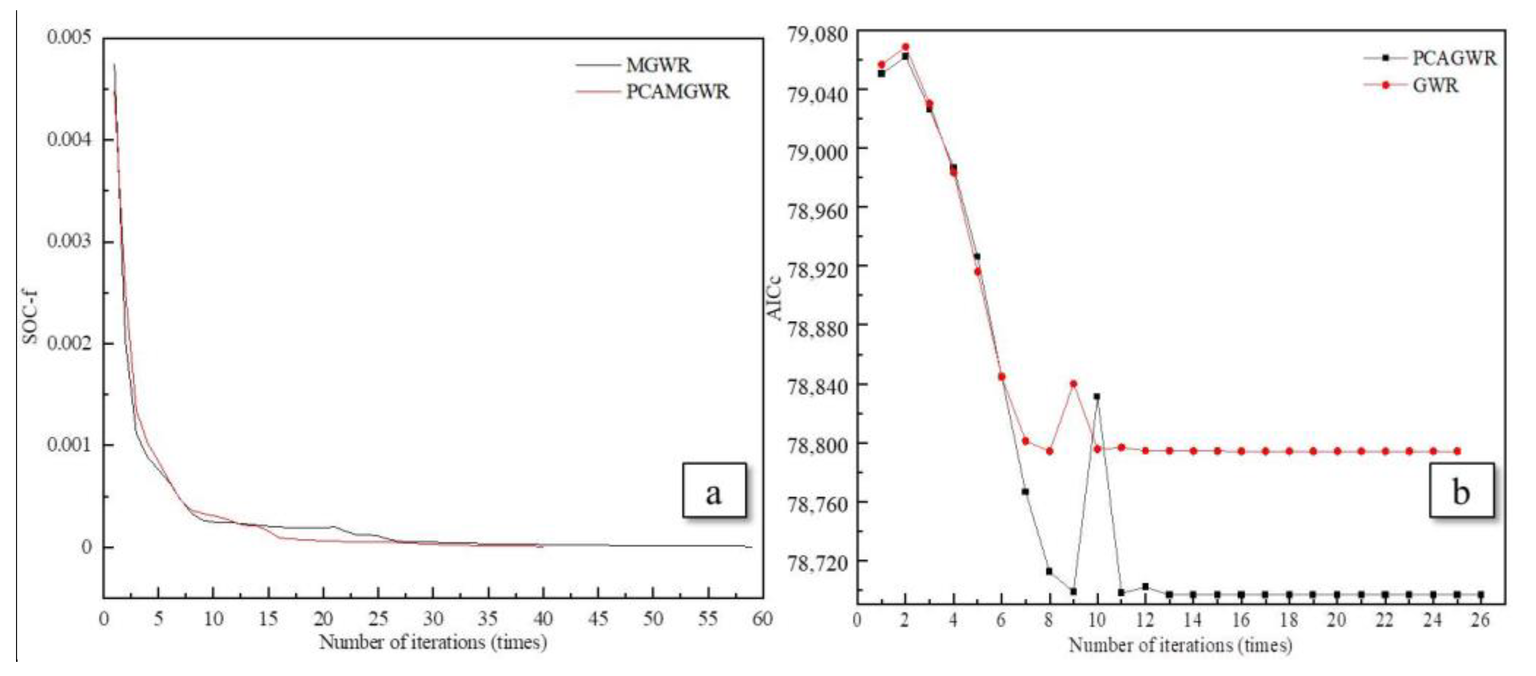
Area under the ROC for different models. Figure 14a shows the convergence of SOC-f during the fitting of the back-fitting algorithm for the MGWR model and PCAMGWR model. The speedy convergence rate means that bandwidth was not chosen at each iteration step, and the optimization stopped at convergence inversely. It can be seen from Figure 14b that the optimal bandwidth was selected based on AICc at a slow convergence, and the AICc value did not continue to decline. It is hard to differentiate the SOC-f of PCAMGWR and MGWR models in detail, and the PCAGWR model represented by the black dot plot was better than the GWR model regarding the convergence of AICc values.
Figure 13.
Area under the ROC for different models. Figure 14a shows the convergence of SOC-f during the fitting of the back-fitting algorithm for the MGWR model and PCAMGWR model. The speedy convergence rate means that bandwidth was not chosen at each iteration step, and the optimization stopped at convergence inversely. It can be seen from Figure 14b that the optimal bandwidth was selected based on AICc at a slow convergence, and the AICc value did not continue to decline. It is hard to differentiate the SOC-f of PCAMGWR and MGWR models in detail, and the PCAGWR model represented by the black dot plot was better than the GWR model regarding the convergence of AICc values.

Figure 14.
Parameter variation diagram of bandwidth judgment criterion: (a) SOC-f for MGWR and PCAMGWR, (b) AICc for GWR and PCAGWR.
Figure 14.
Parameter variation diagram of bandwidth judgment criterion: (a) SOC-f for MGWR and PCAMGWR, (b) AICc for GWR and PCAGWR.


Table 1.
Multicollinearity test of LCFs.
| LCFs | VIF | TOL |
|---|---|---|
| Lithology | 1.328 | 0.753 |
| Distance to stream | 1.109 | 0.901 |
| Distance to settlement | 2.255 | 0.443 |
| Distance to fault zones | 2.195 | 0.456 |
| Aspect | 1.025 | 0.975 |
| Slope | 1.540 | 0.650 |
| Terrain relief | 1.719 | 0.582 |
| Vegetation cover type | 1.019 | 0.981 |
| Precipitation | 1.052 | 0.950 |
| Elevation | 2.861 | 0.350 |
Table 2.
Component matrix of LCFs.
| LCFs | PC1 | PC2 | PC3 | PC4 | PC5 | PC6 |
|---|---|---|---|---|---|---|
| Lithology | 0.500 | −0.448 | −0.160 | 0.109 | −0.211 | 0.176 |
| Distance to stream | 0.272 | 0.322 | 0.542 | 0.156 | 0.071 | −0.621 |
| Distance to settlement | 0.782 | −0.267 | 0.120 | −0.018 | −0.012 | −0.065 |
| Distance to fault zones | 0.803 | −0.291 | 0.097 | 0.003 | −0.084 | 0.163 |
| Aspect | 0.058 | 0.396 | 0.031 | 0.509 | −0.740 | 0.088 |
| Slope | 0.483 | 0.630 | −0.337 | 0.027 | 0.182 | 0.171 |
| Terrain relief | 0.604 | 0.528 | −0.286 | −0.042 | 0.227 | 0.075 |
| Vegetation cover type | −0.034 | −0.277 | −0.190 | 0.819 | 0.450 | −0.058 |
| Precipitation | −0.012 | 0.164 | 0.740 | 0.109 | 0.232 | 0.592 |
| Elevation | 0.865 | −0.086 | 0.112 | −0.084 | 0.000 | −0.147 |
Table 3.
Accuracy statistics of models.
| Model | AIC | AICc | BIC | AUC |
|---|---|---|---|---|
| PCAMGWR | 78,228.039 | 78,291.042 | 85,829.127 | 0.89773 |
| MGWR | 78,232.004 | 78,295.213 | 85,845.297 | 0.89771 |
| PCAGWR | 78,682.364 | 78,696.459 | 82,307.355 | 0.83198 |
| GWR | 78,785.304 | 78,794.218 | 81,672.072 | 0.81701 |
Publisher’s Note: MDPI stays neutral with regard to jurisdictional claims in published maps and institutional affiliations. |
© 2022 by the authors. Licensee MDPI, Basel, Switzerland. This article is an open access article distributed under the terms and conditions of the Creative Commons Attribution (CC BY) license (https://creativecommons.org/licenses/by/4.0/).
Share and Cite
MDPI and ACS Style
Li, Y.; Huang, S.; Li, J.; Huang, J.; Wang, W. Spatial Non-Stationarity-Based Landslide Susceptibility Assessment Using PCAMGWR Model. Water 2022, 14, 881. https://doi.org/10.3390/w14060881
AMA Style
Li Y, Huang S, Li J, Huang J, Wang W. Spatial Non-Stationarity-Based Landslide Susceptibility Assessment Using PCAMGWR Model. Water. 2022; 14(6):881. https://doi.org/10.3390/w14060881
Chicago/Turabian StyleLi, Yange, Shuangfei Huang, Jiaying Li, Jianling Huang, and Weidong Wang. 2022. "Spatial Non-Stationarity-Based Landslide Susceptibility Assessment Using PCAMGWR Model" Water 14, no. 6: 881. https://doi.org/10.3390/w14060881
Note that from the first issue of 2016, this journal uses article numbers instead of page numbers. See further details here.