Geospatial Assessment of Groundwater Quality with the Distinctive Portrayal of Heavy Metals in the United Arab Emirates

Abstract

Groundwater is a valuable resource, and its quality is critical to human survival. Optimal farming and urbanization degraded groundwater reserves. This research investigates and reports the spatial variability of selected heavy metals developed in the Liwa area of the United Arab Emirates. Forty water samples were collected from existing wells and analyzed for different elements. Principal components analysis was applied to a subgroup of the data set in terms of their usefulness for determining the variability of groundwater quality variables. Geographic information systems were used to produce contour maps to analyze the distribution of heavy metals. Ordinary kriging was used with Circular, Spherical, Tetraspherical, Pentaspherical-Bessel, K-Bessel, Hole effect, and Stable models for better representation. The water quality index was constructed using heavy metal concentrations and other variables. This yielded a value of 900 beyond the limit stated by WHO and US EPA. Nugget analysis showed that Cd (0), K (7.38%), and SO₄ (1.81%) variables exhibited strong spatial dependence. Al (27%), Ba (40.87%), Cr (63%), Cu (34%), EC (27%), HCO₃ (56%), NO₃(36%), Pb (64%), and TDS (53%) represented moderate spatial dependence. As (76%), Mn (79%), Ni (100%), pH (100%), Temp (93%), and Zn (100%) exhibited weak spatial dependence.

1. Introduction

Groundwater reaches the aperture of the landmass and its interior through natural, artificial, and indirect recharge. It was used by at least 2 billion people [1]. This infringement of this precious resource can be attributed to its nearest obtainability with partial efforts and spatial obstinacy. Aquifers at specific demand locations are being drained, and this state may lead to deprivation of this indispensable resource unless allayed [2]. The hydraulic conductivity and permeability of the rocks depend on the rocks’ porosity [3]. Heavy metals are among the most significant pollutants of groundwater sources [4,5]. Nonetheless, the toxicity of heavy metals depends on their concentration levels in the environment. With increasing concentrations in the environment and decreasing soils’ capacity toward retaining heavy metals, they leach into groundwater and soil solution [6,7]. Then, these toxic heavy metals can be accumulated and concentrated via the food chain in living tissues [8]. Some of these heavy metals are Arsenic (As), Lead (Pb), Nickle (Ni), Chromium (Cr), and Zinc (Zn). They can be categorized as critical heavy metals that pollute groundwater and affect human health [9]. One of the advanced techniques used in groundwater quality data interpolation is geostatistics [10]. The results obtained from the geostatistics can help a decision-maker to adopt suitable remedial measures to protect the quality of groundwater sources [11].

Focus has been devoted to studying groundwater quality and quantity to prevent groundwater contamination [12]. The native hydrogeological conditions and pollutant loads are dependent on lateral physicochemical interactions on the surface and sub-surface. Geostatistical analysis is used in subjecting data to interpolate by understanding the resemblances [13]. Radial functions and inverse distance weighted values are significant in data smoothing [14]. We can investigate uncertainties and produce surface predictions to get related information without subjecting data to erroneous functions and unnecessary manipulations. The geostatistical tools help us understand data in graphical forms while maintaining the native peaks and troughs, as witnessed by field reports [15]. Three-dimensional visualization evolved as an in-silico currency to reveal native information about the local geology and visualization thereof [16]. The sample points measured spatially can be used in the autocorrelation process in the ordinary kriging method [17]. The association between the transformation between the measured and predicted values can be described with a semi variogram [18]. Semi variance is the product of slope that appears within a fitted model and distance between the location pairs. Geostatistical techniques improved the spatial data distribution with delimited accuracy while maintaining portability [19]. Primarily, spatial analysis mandates the use of GIS and statistics. GIS apparatus is expected to deliver predictions and improved interpretation accuracy per se. Though technical constraints limit us, we can present a near-accurate portrayal of processes and features with GIS tools equipped with geostatistics [20].

Inverse distance weighting (IDW) can be stated as a simple interpolation technique. The weighted average is considered within a neighborhood in IDW [21]. The analyst can regulate a specific mathematical form of the weight function and the neighborhood size [22]. It is necessary to consider IDW with natural neighbor in analyzing substantial data sets. It uses cluster scatter points to identify datasets under investigation. This method is apt for discrete sample data [23].

The geostatistical analysis such as ordinary kriging provides insights into the groundwater situation. Kriging assumes that random processes with spatial autocorrelation can mimic at least some of the spatial variation observed in natural events and that the spatial autocorrelation must be explicitly modeled. However, it has much versatility as a simple prediction tool. An integrated approach to the assessment combining aquifer-based preselection criteria and multivariate non-parametric geostatistics was proposed to overcome the traditional approach’s limitations and include the intrinsic hydrogeological and geochemical heterogeneity into the definition of groundwater water quality [24]. Arsenic (As) is one of the most harmful inorganic contaminants in water streams for the environment and human health [25]. The correlations between different groundwater quality indices and the causes and impacting variables of groundwater pollution can be tracked using statistical and multivariate techniques [26]. The meta-evaluation of the groundwater quality index was attempted [27]. The quality of groundwater that is being used for irrigation can be affected by several factors [28].

Groundwater is a vital resource for human life. Land use changes and urbanization harmed groundwater. This study examines the geographical variability of selected heavy metals in the UAE’s Liwa region. There were limited studies that used geostatistics to explain the groundwater quality variability across this study area. This work is focused on the application of the geostatistical tools to explain the groundwater contamination. The objectives of this study are: (1) To describe the geospatial relationship between the observed groundwater variables using geostatistics, and multivariate analysis; (2) To determine the parameters’ variability at various sample points spread over the study area. PCA was used to define the parameters controlling the groundwater chemistry and the information using significant variables was revealed; (3) To investigate the suitability of water for drinking (Using Weighted Arithmetic Water Quality Index (WA-WQI); (4) To employ ordinary kriging and select an appropriate model representing spatial distribution and spatial dependence variables.

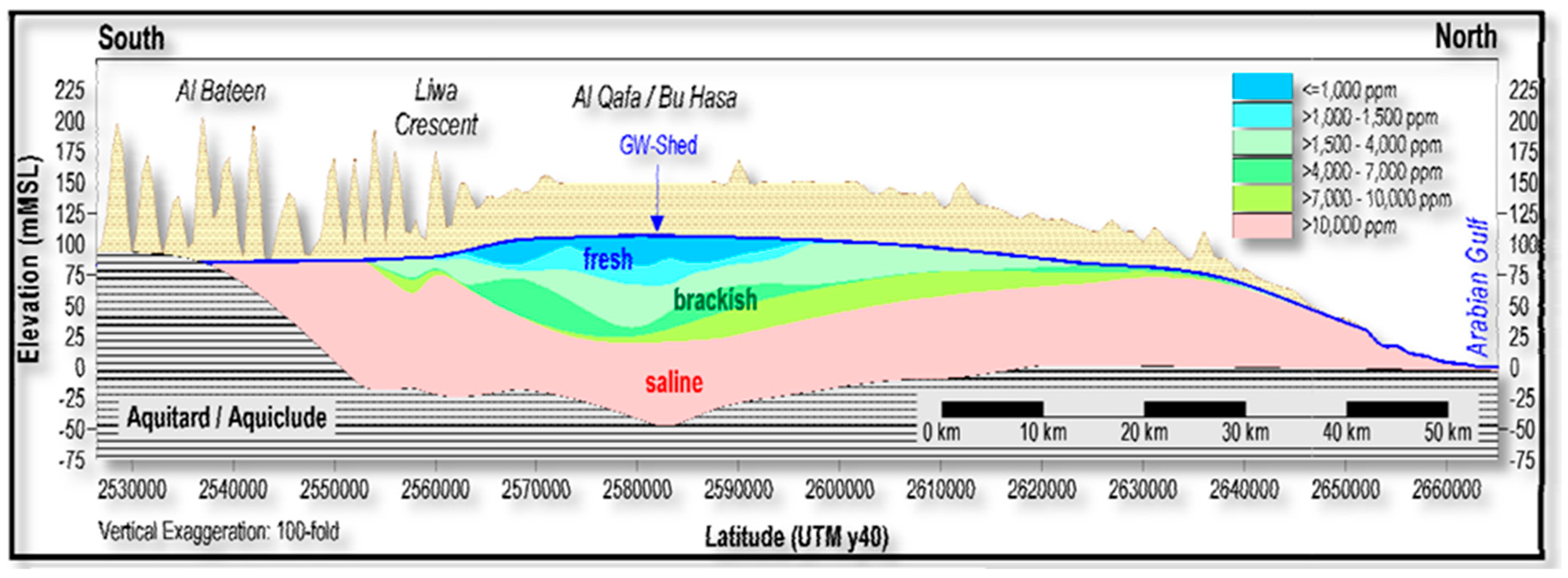
2. General Characteristics of Study Area

The primordial settlements in Abu Dhabi traced to 7000 years ago and elsewhere are regarded as from the late stone age [29]. Agricultural hubs were established by the semi-nomadic peoples at Al Ain and Liwa regions [30]. It is an elapsed statistic that most of the populace endured on sustainable water management, attributed to rough climatic conditions that prevailed then. Stringent punishments were levied on anyone who accidentally or purposely threatened the water resources. The Liwa desert accommodates high temperatures ranging from 40 to 50 °C [31]. We can witness the highest dunes southwards of the Liwa crescent, prevalently known as the Moreeb dune [32]. Though dry scape appears on the surface, dunes can aid in excellent groundwater recharge with whatever rainfall is available over this zone. In the northern side of Liwa, i.e., Madinat Zayed, we can witness fresh water under the dunes [33].

Hydrogeology

The hydraulic conductivities measured at Liwa Crescent and Madinat Zayed ranged from 10–100 m/d. They were marked as a peak in Abu Dhabi. This property can be attributed to the sands that are unconsolidated and homogeneous. In the north of Liwa, water is of low salinity. It was classified as old water as it arrived at the aquifer long ago. Most of the groundwater levels are shown at the agricultural zones of Liwa with high nitrate concentrations [34]. The farm soils of Liwa are Torripsamments with no specific profile [35]. The agricultural activity in this area depends on desalinated water, and hence the native soils are less saline. The Liwa region can be considered an essential food production zone in the United Arab Emirates. Its water reserves are abundant for agriculture. The aquifer beneath this region has become vulnerable to pollution, attributed to several factors. The annual precipitation is confined to the winter season accounting for 100 mm/year [36]. The groundwater recharge is just 4%, and this area is devoid of surface water resources. The Liwa region is being degraded due to excess salinity. Its aquifer lodges increased levels of chromium derived from natural resources.

The Liwa aquifer can be categorized as lens-shaped and with a thickness of 121 mm. The average transmissivity was observed as 300 m²/day [37]. The groundwater movement was observed in the north and south, especially in low-lying areas like sabkha physio-graphic regions, dunes, and sand salt flats [38]. Barchan dune complexes border the Liwa oasis at the south. There is a gradual incline passing to Oman’s Hajjar massif mountain. The oil and gas-related activities injected brine into the groundwater zone. Ummer, Radhuma, Dammam, and Miocene are important aquifers underlying the Liwa region. Rus and Lower Fars were designated as confining units of this area [39]. Limestone dominates Ummer Radhuma and Dammam. Figure 1 shows the hydrogeological cross section of the Liwa region.

Miocene aquifer is dominated by sandstone. There is minimal silt and clay at the upper zones of the soil, resulting in high transmissivity and porosity. The Liwa area is hydrologically unique in the western region, making it a highly productive groundwater resource. Under the Liwa lens, it was observed that 38 bcm (billion cubic meters) of groundwater with TDS greater than 15,000 mg/L is present [40]. Since this aquifer is limited with its connectivity with adjoining aquifer systems, most of the solutes observed might be of atmospheric origins. The recharge of this shallow aquifer is negligible. The flow will be confined to the upper aquifer during intense precipitation especially in unsaturated zones [41]. Unmitigated irrigation-related activities are dumping nitrates into the aquifers. The freshwater lens is being depleted in the Liwa area due to several agricultural activities per se. Liwa oasis provided an agricultural base for the semi-nomadic Bani Yas community. This led to settlements on a large scale in Abu Dhabi [42]. The groundwater studies using geostatistics of the study area were attempted previously and concluded that the anthropogenic and natural processes affected the quality of the groundwater [43,44].

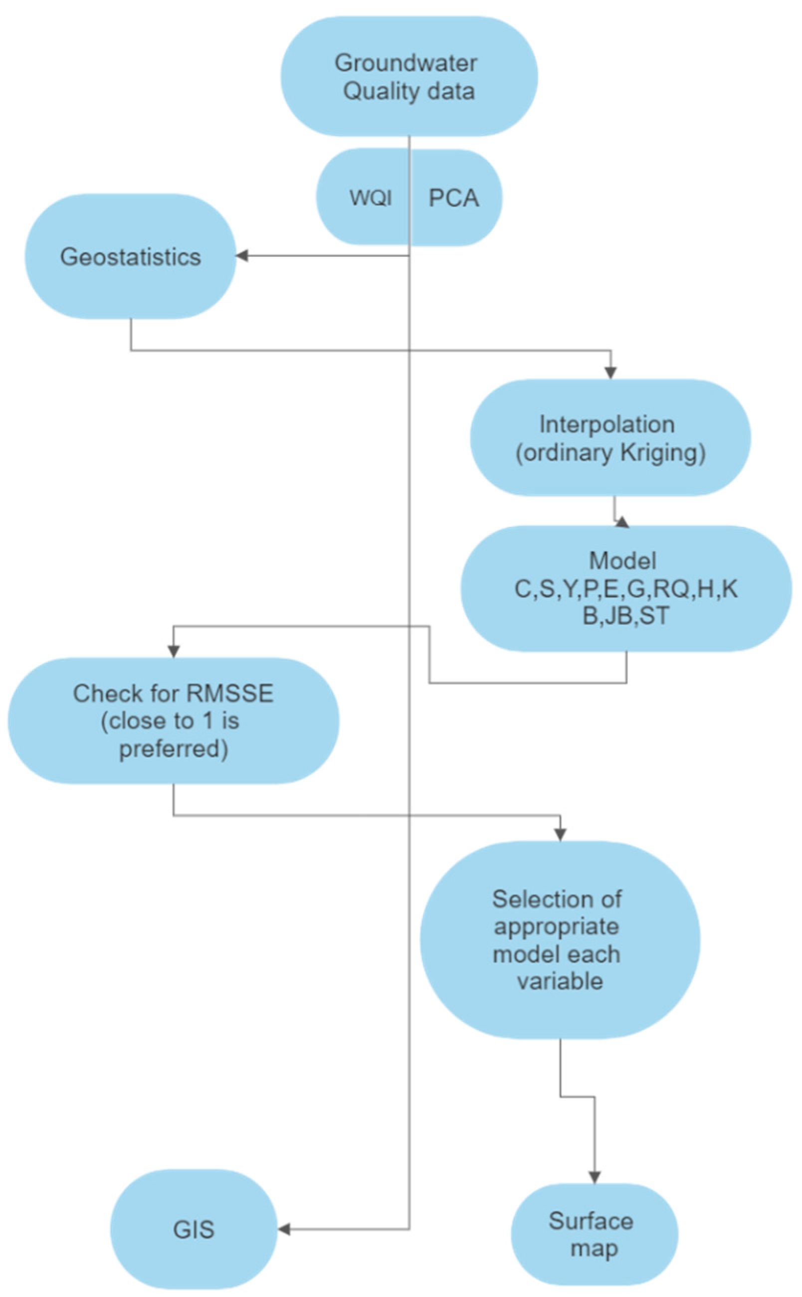
3. Materials and Method

3.1. Sampling and Analysis

The groundwater samples were collected from the Liwa region of the UAE. Forty samples were collected from the study area, and their hydrogeochemical parameters were analyzed. The water samples were analyzed using the American Public Health Association (APHA) standards [45]. The Inductively Coupled Plasma—optical emission spectroscopy (ICP-OES, Avio 200, Perkin Elmer, Waltham, MA, USA) was used to quantify the heavy metals present in groundwater samples. The correlation coefficient and PCA were determined to know the correlation between the elements in the sample. After analyzing the database, the spatial distribution of quality parameters was obtained using ArcGIS 10.8 software to create spatial and layered maps. Semi-variograms were prepared and an appropriate model selected based on the nugget analysis to establish spatial dependence.

Polyethylene bottles of 1 L capacity were used to collect the samples. In order to minimize the risk of contamination, the plastic bottles were rinsed with distilled water prior to being filled with sampled water. The samples were preserved with 65% nitric acid (HNO3) for a pH of 2, and bottles were kept cool at 4 °C. ICP-OES system was used to study the heavy and trace elements (As, Cr, Al, Mn, Ni, Cu, Pb, Zn, Cr, and Cu). Potassium (K), Calcium (Ca), Nitrate (NO₃), and Sulfate (SO₄) were analyzed using Ion Chromatography (ICS 5000+, Thermo Fisher, Waltham, MA, USA). Bicarbonate was determined by titration. Analyses were conducted in duplicate to minimize manual and instrumental errors.

3.2. Water Quality Index (WQI)

There have been many water quality assessment methods proposed by international scholars, such as set pair analysis [46,47,48], rough set and TOPSIS [49,50,51,52], entropy water quality index [53,54,55]. However, water quality index (WQI) is the most popular and widely adopted methods for overall water quality assessment [56,57]. In this study, the water quality index (WQI) was constructed using the weighted arithmetic average method as shown below [58].

$$Calculation for water quality rating(Q_n)=100\times \frac{(V_n-V_0)}{(S_n-V_0)}$$

(1)

Q_n: Water quality rating for the nth parameter, V_n: Observed value of the nth parameter, V₀: Ideal value, S_n: Standard permissible value of nth parameter.

The unit weight of the corresponding parameter was an inverse proportional value to the recommended standard value of S_n

$$\mathrm{Calculation}\mathrm{of}\mathrm{unit}\mathrm{weight}\left(W_n\right)=\frac{K}{S_n}$$

(2)

W_n: unit weight for the nth parameter, S_n: standard value of the n th parameter, K is the constant for proportionality: K = $\frac{1}{\Sigma \frac{1}{S_n}}$

The total water quality index was calculated linearly by adding the quality rating to the unit weight:

$$\mathrm{WQI}={\displaystyle \sum }{Q}_n{W}_n/{\displaystyle \sum }{W}_n$$

(3)

3.3. Principal Component Analysis (PCA)

PCA is one of the popular statistical analysis techniques that can be used to investigate data patterns. The Principal Components Approach can be assumed as a comprehensive Factor Analysis method. The goal of principle component analysis (PCA) is to construct new variables, known as principal components, from a set of existing original variables [59,60]. The new variables are created by linearly combining the current variables. The PCA reduces an extensive data set of variables into a few elements known as the principal components, which can then be analyzed to show the underlying data structure. It is one of the features of primary components that they are not correlated or orthogonal with one another. When a data set has a significant variance, the first principal component (F1) absorbs and accounts for as much variance as feasible. The second component (F2) absorbs the remaining variation as feasible, and so on. The maximum number of PCs or principal components equals the total number of variables in a model unless otherwise specified. Because each standardized variable has one variance, the total variance accounted for by all of the Fi’s will be equal to the number of variables. Only a few Fi numbers are maintained in the data processing process to facilitate comprehension. The Kaiser criterion determines the number of primary components preserved in the analysis. It is also possible to express the latent root as a proportion of the overall variance in the data set. The diagram showing methodology is given in Figure 2.

4. Results and Discussion

4.1. Water Quality Index

The water quality index is represented in

Table 1. Water Quality Index.

Parameters	Vn	V0	Sn	Wn	Qn	WQI
Cr	0.015	0	0.05	20.000	29.523	29.523
Cu	0.002	0	2	0.500	0.079	0.079
K	8.964	0	20	0.050	44.820	44.820
Mn	0.002	0	0.4	2.500	0.589	0.589
Zn	0.005	0	3	0.333	0.156	0.156
Ba	0.166	0	0.7	1.429	23.704	23.704
As	0.022	0	0.01	100.000	220.996	220.996
TDS	863.049	0	500	0.002	172.610	172.610
EC	1478.488	0	400	0.003	369.622	369.622
NO3	1.410	0	5	0.200	28.200	28.200
SO4	23.570	0	250	0.004	9.428	9.428
pH	6.519	7	8.5	0.118	−32.065	−32.065
HCO3	87.546	0	350	0.003	25.013	25.013
Total						900.52

. Water quality classification based on WQI value. If the WQI value is between 0 and 25, it can be considered excellent, and it is good if it falls between 26 and 50. Some other ranges, including 51–75 (poor), 76–100 (very poor), and >100 (Unfit for consumption). The calculated WQI of this area is 900, and it is way beyond the recommended value.

The descriptive statistics presented in

Table 2. Descriptive statistics.

Variable	Mean	Max	Min	SD
Al	0.990	1.450	0.339	0.233
As	0.022	0.029	0.008	0.004
Ba	0.166	0.457	−0.065	0.136
Cd	0.181	0.183	0.175	0.002
Cr	0.014	0.023	0.48 × 10–3	0.006
Cu	0.001	0.004	0.873 × 10−3	9.351 × 10−4
EC	1478.488	3003	328	656.631
HCO3	87.546	236.680	14.640	49.449
K	8.964	17.203	2.704	3.160
Mn	0.002	0.011	0.0002	0.003
Ni	0.001	0.004	0.0004	0.001
NO3	1.410	2.486	0.426	0.557
Pb	0.412	0.490	0.289	0.048
pH	6.519	7.190	6.190	0.259
SO4	23.570	45.794	4.129	9.255
TDS	863.049	1565	136	358.995
Temp	28.378	32.600	23.500	1.741
Zn	0.003	0.051	0.0357 × 10−2	0.008

reflect different mean values for each variable in this dataset. The cadmium concentration ranges from 0.17 to 0.183 ppm with a mean of 0.18, chromium concentration from 0.00048 to 0.023 ppm with a mean of 0.014 ppm, copper concentration from 0.000873 ppm to 0.004 ppm with a mean value of 0.001 ppm, potassium concentration observed to be from 2.704 to 17.202 ppm, with a mean value of 8.964 ppm. The mean value of the manganese concentration was found to be 0.0023 ppm. The Ni concentration ranges from 0.00049 to 0.0044 ppm with a mean value of 0.001 ppm. The Pb concentration ranges from 0.289 to 0.490 ppm with an observed mean value of 0.412 ppm, and the Zn concentration ranges from 0.000357 to 0.051 ppm with a mean value of 0.003 ppm. The mean concentration of Ba and Al is 0.166 and 0.990 ppm, respectively.

Hence, correlation analysis is presented in Figure 3. The correlation analysis was done to investigate the relationships between the parameters measured.

The degree to which two variables are allied is weighed by a correlation coefficient, indicated by the letter r. This coefficient, named after its discoverer, Pearson, measures linear association used in statistics and education. It is necessary to utilize alternative, more though measures of the correlation if a curved line is required to describe the relationship. The correlation coefficient can be measured from + 1 to −1 and is expressed as a percentage. The degree of complete correlation between two variables is represented by the numbers + 1 or −1, respectively. Correlations are positive when one variable increases in response to another’s increase and negative when one variable reduces in response to the other increases. The number zero represents the complete absence of association.

Cadmium is negatively correlated with Cr, K, Pb, TDS, and EC and positively correlated with Mn, Zn, As, and pH. This shows that the heavy metals with pH other than Cd are affecting the Cd concentrations and this can be due to anthropogenic causes. Cr is positively correlated with Cu, K, Ba, Temp, and EC and negatively correlated with Mn, As, NO₃, and HCO₃. This shows that the increase in Cr concentration is associated with the other heavy metals (Antropogenic) along with the EC and temperature (Natural Process). Cu is positively correlated with Zn, Ba, NO₃, Ni (Anthropogenic), EC, HCO₃, and Temp. K exhibits a positive correlation with Mn, Ni, Pb, Al, As, TDS, NO₃, SO₄, and EC and a negative correlation with Zn, Ba, Temp, and pH. Mn positively correlates with Al and As and negatively correlates with Ba and Temp. Ni is positively correlated with Pb, Al, As, TDS, NO₃, SO₄, and EC and negatively correlated with Zn and pH. Pb is positively correlated with Al, As, TDS, NO₃, SO₄, and EC and negatively correlated with Zn, Ba, Temp, and pH. Zn is positively correlated with Al and pH and negatively correlated with Temp and EC. Ba is positively correlated with Temp, pH, and EC and negatively correlated with Al, As, TDS, and HCO₃. Al is positively correlated with As, TDS, NO₃, SO₄, and EC and negatively correlated with Temp and pH. As is positively correlated with TDS, NO₃, SO₄, HCO₃, and EC and negatively correlated with Temp and pH. TDS is positively correlated with NO₃, SO₄, and EC and negatively correlated with HCO₃, Temp, and pH. NO₃ is positively correlated with SO₄, HCO₃, and EC and negatively correlated with Temp and pH. SO₄ exhibits a negative correlation with HCO₃, Temp, and pH and positively correlates with EC. HCO₃ is negatively correlated with pH and EC.

The observed cadmium value is 0.18 ppm in the study area. This water might not suit agriculture, irrigation, and drinking purposes. The increase in cadmium levels can be due to sewage sludge, fertilizers, battery alloys, and cigarette smoking. The increased levels of Cd can damage kidneys. Due to this, there will be disruption of the endocrine system and inhibition of sex hormones in humans. Long-time exposure to Cadmium may cause Itai-itai in humans. The recommended chromium standard in drinking water is 0.1 ppm (EPA) and 0.05 ppm (WHO). The maximum value of chromium in the water sample is 0.023, which is well within the permissible limits. Cu (0.004), Mn (0.01), Zn (0.051), Ba (0.457), NO₃ (2.4), SO₄ (45), Temperature (32.6), pH (7.19), and bicarbonates are within the normal range specified by WHO and US EPA. The EC values are at 3003, and it is problematic. Pb (0.49), As (0.028), and Al (1.45) are high in the water samples collected from the study area. The concentration of Cadmium in the observed samples is 0.184 (0.183984), and this is higher than the WHO recommended value of 0.003 mg/L. The concentration of lead observed in the groundwater samples is 0.4905 mg/L against 0.01 mg/L (WHO). The concentration of Aluminum in the samples analyzed is 1.4502 and is higher than the WHO recommended value of 0.9 mg/L.

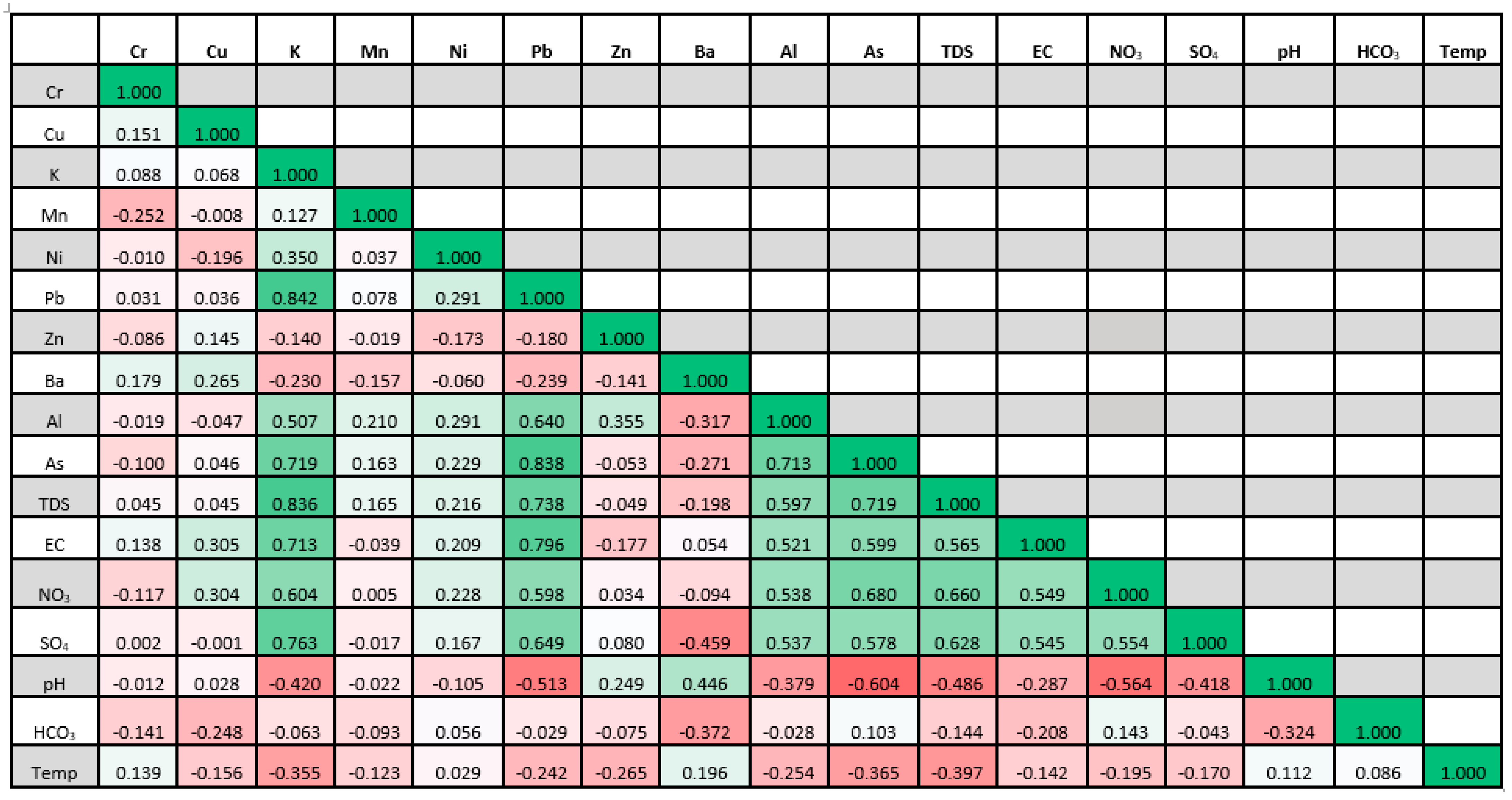
4.2. Principal Component Analysis

Pearson correlation matrices and PCA construed the datasets. Principal components were generated using varimax rotation, and this yielded variables that contribute more and other variables that contribute less. Multi-variate analysis was used in the PCA to transform a significant set of correlated variables into a minor set of uncorrelated variables. The interrelationships among the variables can be highlighted using covariance by this tool, and it is also called a dimensionless reduction tool. We can use PCA to know the associated chemicals construed as variable loadings on certain groundwater quality factors. Two significant eigenvalues, i.e., PC1 and PC2, were observed in the 40 groundwater samples with 18 parameters, constituting 35 and 12% of the variance. PC3 exhibited 10% of variance but PC4 and PC5 exhibited variance less than 10%. The first five components exhibited eigenvalues that are greater than 0.5. It is assumed that the factor loading value near +/− 1 exhibits a strong correlation. If the value if greater than 0.5, it is significant. PC1 exhibits 35% of variance about significant loadings of K, Pb, Al, As, TDS, nitrate, sulfate, and pH, and is shown in

Table 3. Principal Component Loadings.

Variable	PC1	PC2	PC3	PC4	PC5	Uniqueness
Cd			0.739			0.387
Cr			−0.680			0.489
Cu					0.841	0.203
K	0.908					0.156
Mn			0.709			0.412
Ni					−0.522	0.527
Pb	0.919					0.140
Zn				0.889		0.174
Ba		0.618				0.274
Al	0.708			0.405		0.288
As	0.868					0.156
Nitrate	0.867					0.231
Sulfate	0.768					0.246
HCO3	0.738	−0.836				0.336
Temp						0.270
pH	−0.572	0.626		−0.524		0.586
EC	0.810					0.254
						0.204

.

PC2 showed 12% variance associated with significant loadings of Ba, HCO₃, and pH. The component characteristics and component loadings for this data are presented in Table 3 and

Table 4. Component characteristics.

Variable	Model	Nugget Ratio (%)
Cd	S *	0
Cr	P	63.456
Cu	C	34.148
K	RQ	7.384
Mn	G	79.008
Mn	S *	79.008
Pb	J	64.935
Zn	H	100
Ba	H	40.879
Al	RQ	27.089
As	G	76.753
As	S *	76.753
Sulfate	T	1.817
HCO3	J	56.035
Temp	H	93.559
PH	C	100
EC	J	27.262
Ni	C	100
NO3	H	36.387
TDS	J	53

S * = stable model.

. PC2 is loaded with Ba, HCO₃, and pH, whereas PC3 is loaded with Cd, Cr, and Mn. PC4 is loaded with Zn, Al, and pH and PC5 is loaded with Cu and Ni. Temperature, Cr, Ni, and Mn exhibited higher uniqueness values, suggesting that these variables have limited commonality. As evidenced by systematic data analysis, PC1 exhibited significant cations and anions due to anthropogenic and natural sources.

The cos values are employed to know the representation’s quality, and the individuals closer to the center of the plot are assumed of limited or low importance for the reported first components. The low cos values are shown in blue and high cos values in red (Figure 4). The contribution of the variables with sample points is presented in Figure 5.

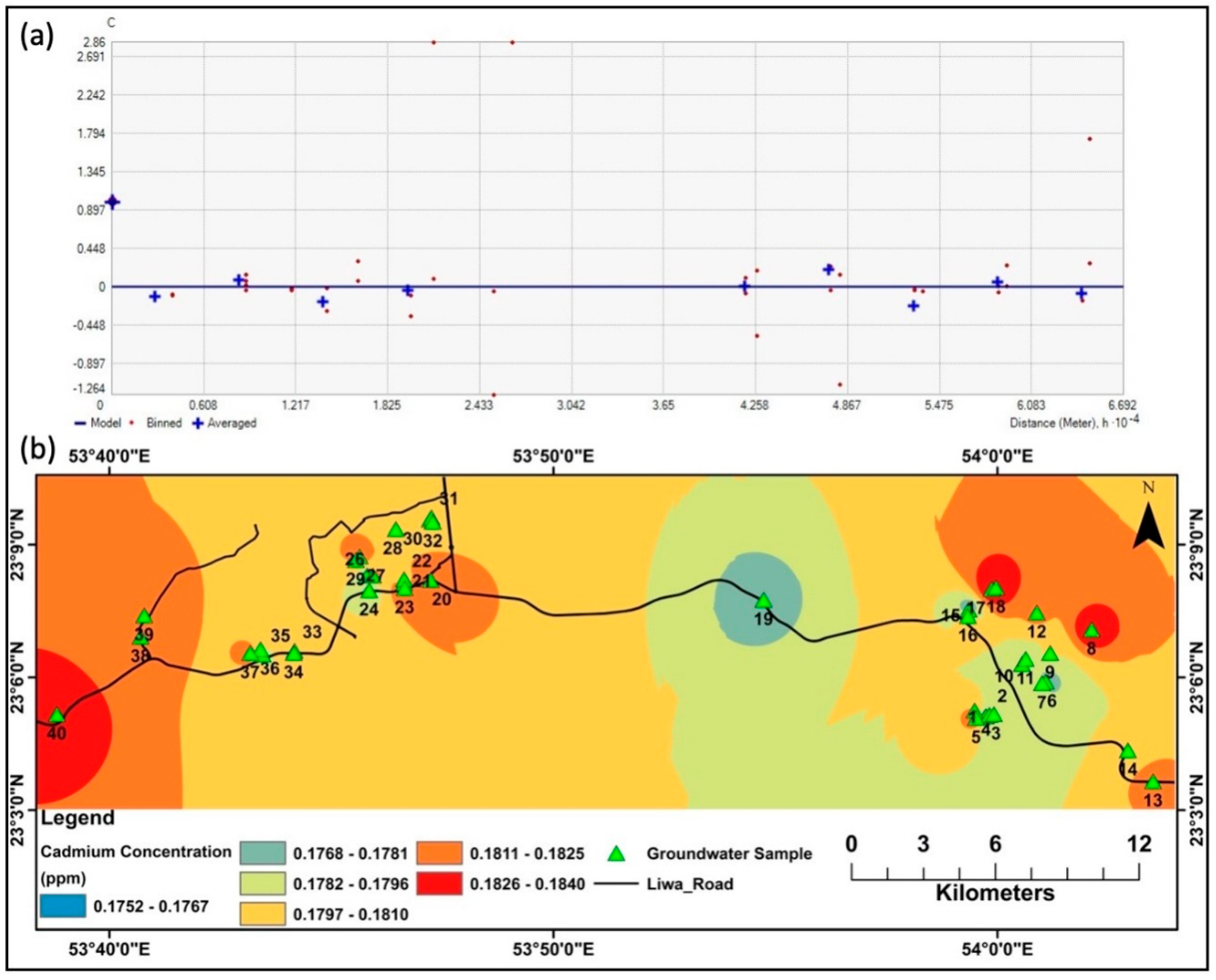
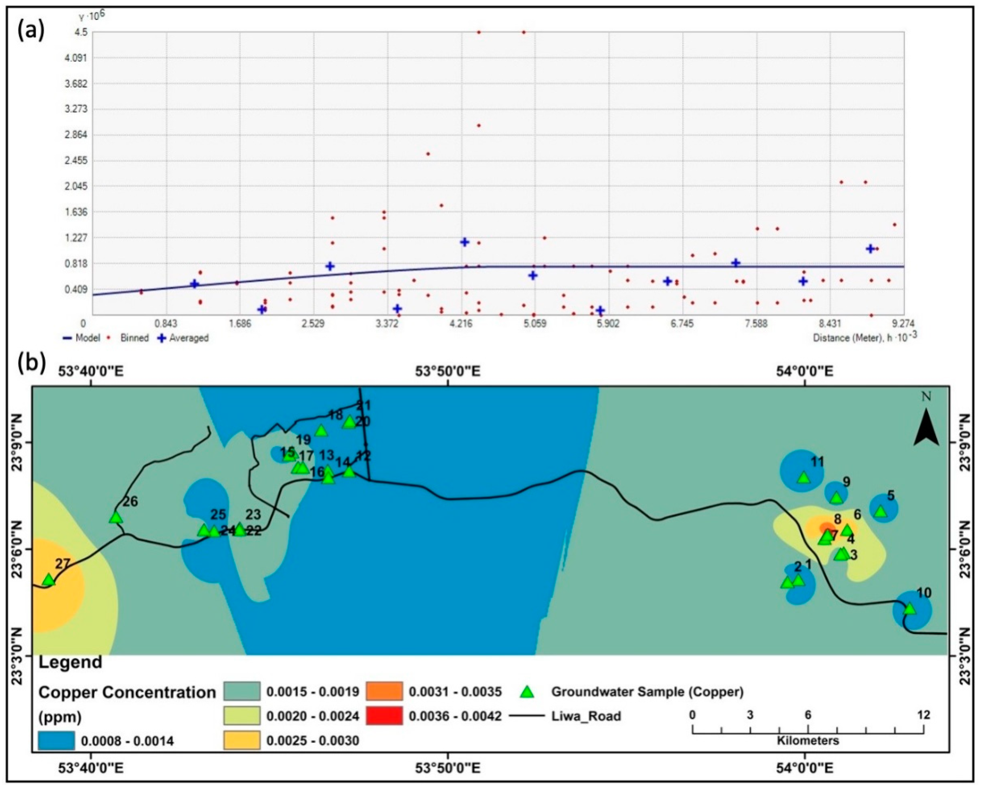
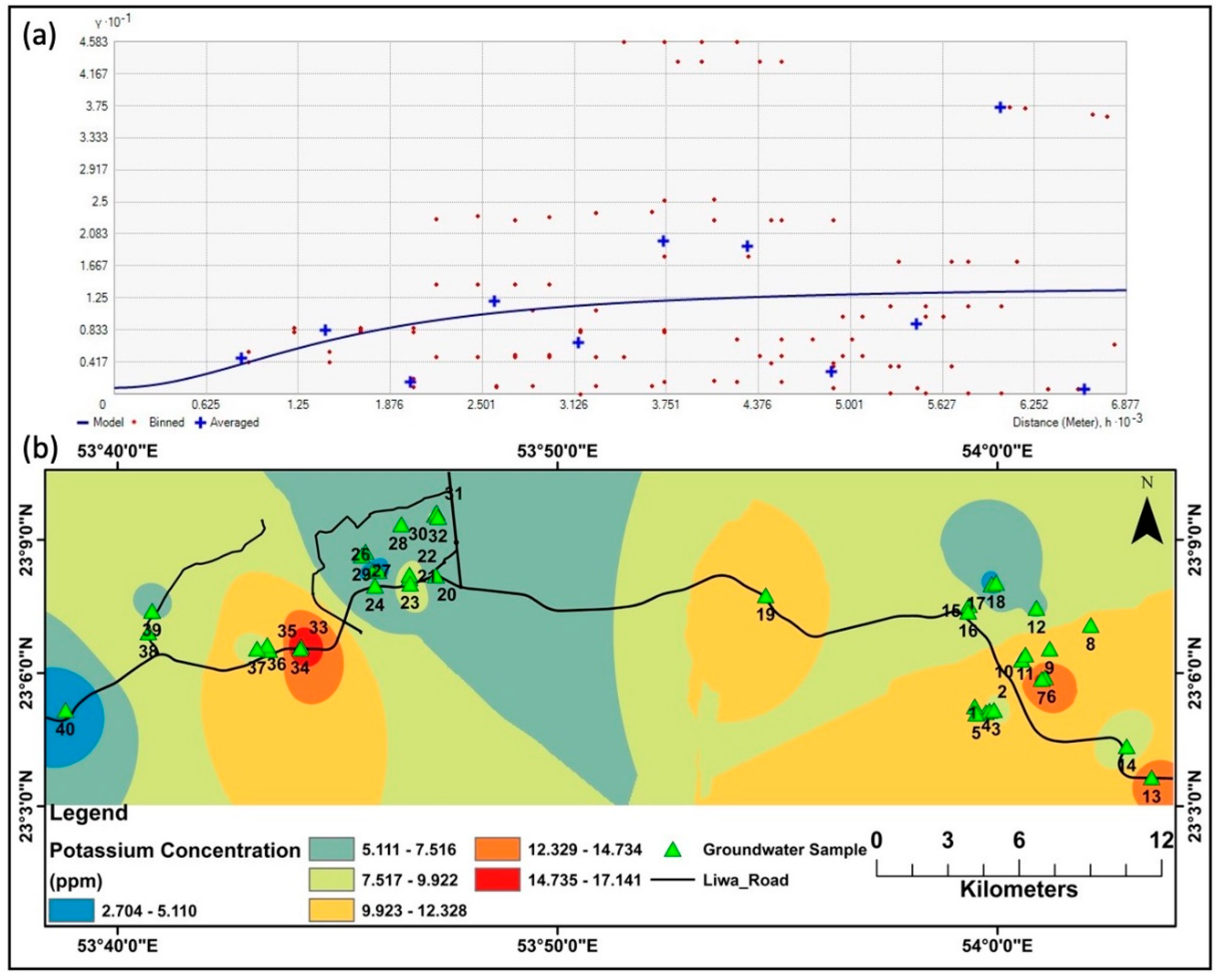
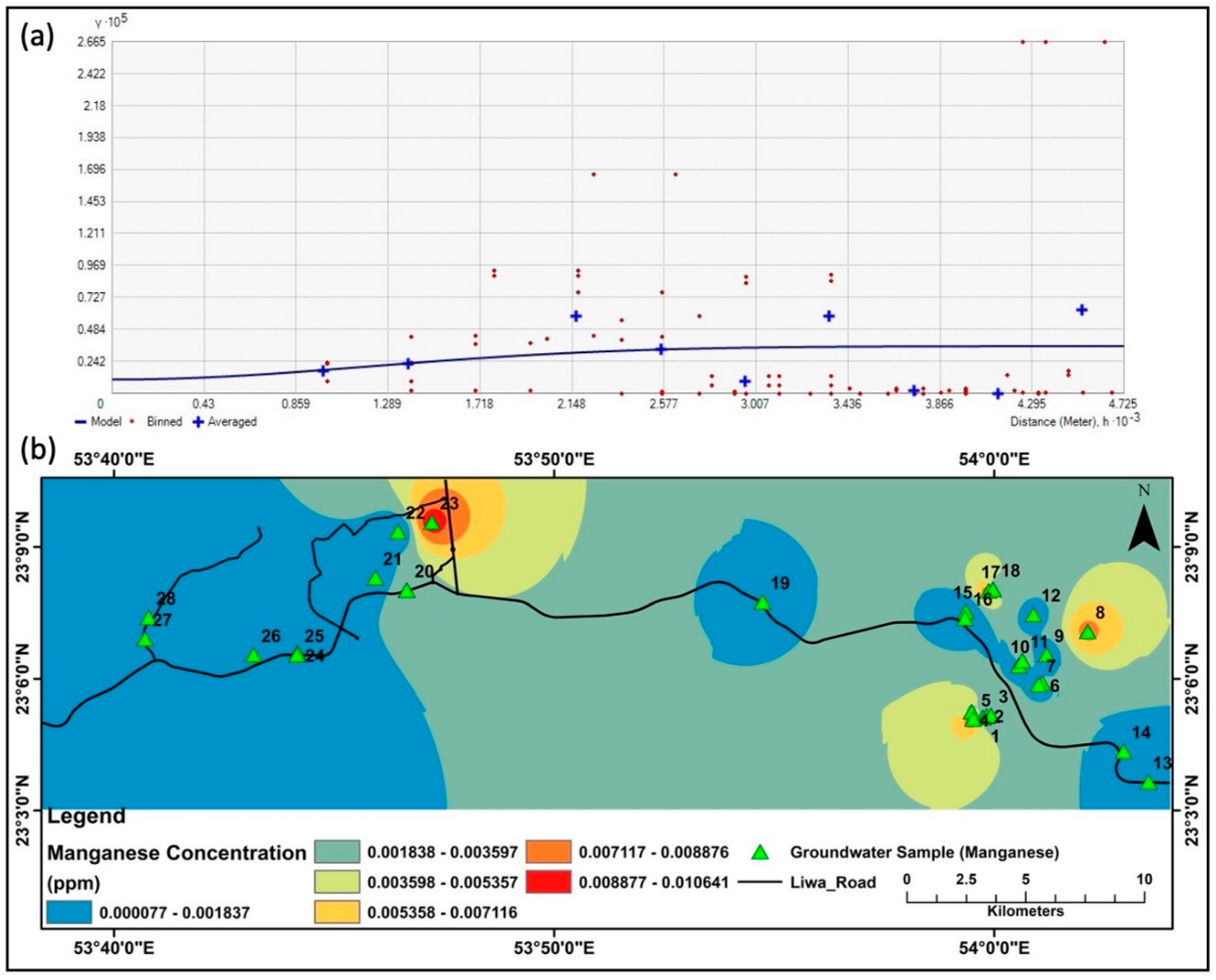
4.3. Geostatistical Analysis of the Study Area (Spatial Distribution)

The statistical and geostatistical analysis was done using ArcGIS 10.2, R, R studio, and MS Excel 2019. The spatial interpolators can easily predict the values of a specific attribute at locations unknown to the observer utilizing the values of sample locations known previously. The deterministic interpolators can utilize mathematical formulae to know the predicted values. This can be interpreted as similarity among the neighboring points and smoothing extent. The geostatistical interpolation techniques use certain statistical properties of the points previously measured to estimate the value of the surface locations. Depending on the spatial structure of the datasets framed, we can investigate the spatial dependence among the variables. The ordinary kriging method was selected based on a comparative analysis of interpolation methods. Models such as Circular (C), Spherical (S), Tetraspherical (T), Pentaspherical (P), Exponential (E), Gaussian (G), Rational Quadratic (RQ), Hole effect (H), K-Bessel (K), J-Bessel (J), and Stable (S*) were used to arrive at appropriate semi variogram. The best-fitted models are RQ (Al and K), G (As), S* (As, Cd, and Mn), H (Ba, NO₃, Temp, Zn), P (Cr), C (Cu, Ni, and pH), and J (EC, HCO₃, Pb, and TDS). Suppose the nugget ratio is less than 25%. In that case, we can assume that there is strong spatial dependence; 25 to 75% can be reflected as moderate spatial dependence. If greater than 75%, we can expect least or weak spatial dependence. After nugget analysis, it is obvious that Cd (0), K (7.38%), and SO₄ (1.81%) variables exhibited strong spatial dependence. Al (27%), Ba (40.87%), Cr (63%), Cu (34%), EC (27%), HCO₃ (56%), NO₃(36%), Pb (64%), and TDS (53%) represented moderate spatial dependence. As (76%), Mn (79%), Ni (100%), pH (100%), Temp (93%), and Zn (100%) exhibited weak spatial dependence. Nugget analysis for selecting the appropriate model was presented in

Table 5. The Spatial distribution and semi variogram element’s observed sites.

S. No	Elements	Low	Moderate	High
1.	Aluminum (Al)	North west	Western end	Eastern end
2.	Arsenic	North west	Western end	South eastern
3.	Barium	Western end	South western and north eastern	South western
4.	Cadmium	Northern end	North-south (extended)	Western end
5.	Chromium	Northern end	North-south (extended)	Western end
6.	Copper	North-south (extended)	Western end	Eastern end
7.	Potassium	Western end	Partially spotted all over the area	North eastern
8.	Manganese	Western end	South east	North west

.

The spatial distribution maps and semi variogram plots of essential variables were presented in Figure 6, Figure 7, Figure 8, Figure 9, Figure 10, Figure 11 and Figure 12. Table 5 shows the specific locations of elements distribution in the area.

The groundwater investigations in this area are expensive, and the sample locations were limited. Efforts are in progress to collect more samples with an increased temporal resolution to cross-validate the results obtained from the actual observations. Geostatistics in groundwater studies was never attempted for this study area. This study integrated physio-chemical, multivariate, and geostatistical analysis and water quality indices to analyze groundwater quality parameters. The parameters were correlated using correlation analysis, and both positive and negative correlations were found. To mention a few, Arsenic is positively correlated with nitrates, sulfates and EC and negatively correlated with pH and temperature. Lead is positively correlated with Al and As and negatively correlated with Ba and Zn. Ni positively correlated with As, Al, and Pb and negatively correlated with Zn. Chromium reflected a positive correlation with Ba and Cu and negatively correlated with As and Mn. Zinc is positively correlated with Al.

A PCA was performed, and the results showed that there were five main components, PC1 through PC5, which represented a variance of 35% (PC1) and 12% (PC2), 10% (PC3), <10% (PC4 and PC5), respectively. Significant loadings on PC1 are As, Al, Pb, K, pH, sulfate, and nitrate. PC2 accommodates significant loadings of Ba and bi-carbonates with pH.

The dataset was subjected to geostatistical analysis, and a suitable model was identified using standard kriging. The J-Bessel model was selected to represent Pb, TDS, HCO₃, and EC. Pentaspherical model is employed to represent Cr. The circular model was used to show the distribution of Ni, Cu, and pH. The hole effect model was used to describe the spatial distribution of Zn, Temp, NO₃, and Ba. A stable model was employed to reflect the distribution of Mn, Cd, and As. The rational quadratic model was used to represent K and Al. Based on nugget analysis, it was observed that Zn, As, Mn, Ni, pH, and TDS exhibited weak spatial dependence. Moderate spatial dependence was exhibited by Al, Ba, Cr, Cu, Ec, HCO₃, NO₃, Pb, and TDS. Strong spatial dependence was observed in Cr, K, and SO₄.

Groundwater quality deterioration has become a nightmare in this region, and this was due to limited surveillance and the never-ending injection of pollutants into this precious source. Most of the populace in this study area rely on this for industrial and drinking purposes after purification. Several studies were made to evaluate the potability of groundwater of Liwa aquifer mainly for agricultural needs; however, rigorous geostatistical methods were sparsely applied. This paper attempts to fill the void left in using geostatistics to represent groundwater quality. The variation among the sample clusters was studied previously using PCA. This paper uses optimal interpolation techniques and semivariogram analysis to produce statistically enriched results. Geological elements, and environmental and hydrological parameters were considered the core of these studies. Previous studies were made to emulate the subsurface hydrology characteristics with limited utilization of the geostatistics, and this work will add valuable inputs to the contemporary research on groundwater situation analysis and management. This paper presents a GIS-based approach with geostatistics in assessing groundwater quality at the Liwa region, UAE. The correlation matrix obtained supports PCA analysis. The results also shed light on groundwater quality deterioration due to anthropogenic activities. The exponential semivariogram model was systematically authenticated for each groundwater parameter. Analysis of groundwater samples reflects that cadmium, aluminum, and lead is in high proportions compared to other parameters like Cr, Cu, K, Mn, Ni, Zn, and Ba. The distribution maps are produced using the appropriate model of the kriging interpolation method for each variable.

5. Conclusions and Recommendation

In the present study, the detailed analyses show that this study offers background information on the groundwater parameters and factors that affect groundwater quality. This paper can aid water resource planners in coming up with management plans to safeguard the local population’s health. The water quality index of this area is poor, and it is to be improved with the immediate inclusion of proposals for the rejuvenation of groundwater.

Liwa aquifer is exploited beyond the reasonable limit. It will permanently change the subsurface landscape in the coming decades. Given the observed water quality parameters, it is proposed that some of the stringent actions must be levied on the exploiters of this jewel of water in the Liwa basin. The water quality index of this region is alarmingly high, and the stakeholders in this region must mitigate the problem with immediate sustainable solutions.

The excess dumping of the wastes and improper groundwater extraction are assumed to be the main reasons behind this physicochemical variability observed in the water samples. The local geology might also affect this variability, and it is yet to be studied over all the study areas. This study combined the multivariate, geostatistical, and physicochemical analysis; however, complete hydrological analysis in the watershed, HRU, etc., could not be conducted. This is attributed to the local non-conducive conditions.

This area is devoid of the undulations and inundations of the terrain with almost indiscriminate relief. The data is collected once, and the second attempt to collect groundwater samples was not feasible due to budgetary and administrative constraints. If this had been materialized, there might have been a more intense comparative study with the dynamics of groundwater quality parameters. Due to the unavailability of the two-date data, there were no attempts to compare pre-monsoon, monsoon, and post-monsoon groundwater quality.

References

1. Maliva, R.G. Aquifer Characterization and Properties. In Aquifer Characterization Techniques: Schlumberger Methods in Water Resources Evaluation Series No. 4; Maliva, R.G., Ed.; Springer Hydrogeology; Springer International Publishing: Cham, Switzerland, 2016; pp. 1–24. ISBN 978-3-319-32137-0. [Google Scholar]
2. Barbulescu, A.; Nazzal, Y.; Howari, F. Assessing the Groundwater Quality in the Liwa Area, the United Arab Emirates. Water 2020, 12, 2816. [Google Scholar] [CrossRef]
3. Park, B.; Kim, K.; Kwon, S.; Kim, C.; Bae, D.; Hartley, L.; Lee, H. Determination of the hydraulic conductivity components using a three-dimensional fracture network model in volcanic rock. Eng. Geol. 2002, 66, 127–141. [Google Scholar] [CrossRef]
4. Guo, Y.; Li, P.; He, X.; Wang, L. Groundwater quality in and around a landfill in northwest China: Characteristic pollutant identification, health risk assessment, and controlling factor analysis. Expo. Health 2022. [Google Scholar] [CrossRef]
5. Nazzal, Y.; Orm, N.B.; Barbulescu, A.; Howari, F.; Sharma, M.; Badawi, A.E.; Al-Taani, A.A.; Iqbal, J.; Ktaibi, F.E.; Xavier, C.M.; et al. Study of Atmospheric Pollution and Health Risk Assessment: A Case Study for the Sharjah and Ajman Emirates (UAE). Atmosphere 2021, 12, 1442. [Google Scholar] [CrossRef]
6. Liu, L.; Wu, J.; He, S.; Wang, L. Occurrence and distribution of groundwater fluoride and manganese in the Weining Plain (China) and their probabilistic health risk quantification. Expo. Health 2021. [Google Scholar] [CrossRef]
7. Wei, M.; Wu, J.; Li, W.; Zhang, Q.; Su, F.; Wang, Y. Groundwater geochemistry and its impacts on groundwater arsenic enrichment, variation, and health risks in Yongning County, Yinchuan Plain of northwest China. Expo. Health 2021. [Google Scholar] [CrossRef]
8. Belkhiri, L.; Narany, T.S. Using Multivariate Statistical Analysis, Geostatistical Techniques and Structural Equation Modeling to Identify Spatial Variability of Groundwater Quality. Water Resour. Manag. 2015, 29, 2073–2089. [Google Scholar] [CrossRef]
9. Sankhla, M.S.; Kumar, R. Contaminant of Heavy Metals in Groundwater & Its Toxic Effects on Human Health & Environment. IJESNR 2019, 18, 1–5. [Google Scholar] [CrossRef]
10. Bodrud-Doza, M.; Bhuiyan, M.A.H.; Islam, S.M.D.-U.; Quraishi, S.B.; Muhib, M.I.; Rakib, M.A.; Rahman, M.S. Delineation of Trace Metals Contamination in Groundwater Using Geostatistical Techniques: A Study on Dhaka City of Bangladesh. Groundw. Sustain. Dev. 2019, 9, 100212. [Google Scholar] [CrossRef]
11. Verma, P.; Singh, P.K.; Sinha, R.R.; Tiwari, A.K. Assessment of Groundwater Quality Status by Using Water Quality Index (WQI) and Geographic Information System (GIS) Approaches: A Case Study of the Bokaro District, India. Appl. Water Sci. 2019, 10, 27. [Google Scholar] [CrossRef] [Green Version]
12. Tyler, S.W.; Muñoz, J.F.; Wood, W.W. The Response of Playa and Sabkha Hydraulics and Mineralogy to Climate Forcing. Groundwater 2006, 44, 329–338. [Google Scholar] [CrossRef] [PubMed]
13. Setianto, A.; Triandini, T. Comparison of Kriging and Inverse Distance Weighted (IDW) Interpolation Methodsin Lineament Extraction and Analysis. J. Appl. Geol. 2015, 5, 21–29. [Google Scholar] [CrossRef]
14. Alsharhan, A.S.; Rizk, Z.E. Conclusions. In Water Resources and Integrated Management of the United Arab Emirates; Alsharhan, A.S., Rizk, Z.E., Eds.; World Water Resources; Springer International Publishing: Cham, Switzerland, 2020; pp. 793–829. ISBN 978-3-030-31684-6. [Google Scholar]
15. Al-Taani, A.A.; Nazzal, Y.; Howari, F.M.; Iqbal, J.; Bou Orm, N.; Xavier, C.M.; Bărbulescu, A.; Sharma, M.; Dumitriu, C.-S. Contamination Assessment of Heavy Metals in Agricultural Soil, in the Liwa Area (UAE). Toxics 2021, 9, 53. [Google Scholar] [CrossRef] [PubMed]
16. Zheng, K.; Li, C.; Wang, F. Gaussian Radial Basis Function for Unsteady Groundwater Flow. IOP Conf. Ser. Earth Environ. Sci. 2019, 304, 022052. [Google Scholar] [CrossRef]
17. Elubid, B.A.; Huang, T.; Ahmed, E.H.; Zhao, J.; Elhag, M.; Abbass, W.; Babiker, M.M. Geospatial Distributions of Groundwater Quality in Gedaref State Using Geographic Information System (GIS) and Drinking Water Quality Index (DWQI). Int. J. Environ. Res. Public Health 2019, 16, 731. [Google Scholar] [CrossRef] [Green Version]
18. Venkatramanan, S.; Viswanathan, P.M.; Chung, S.Y. (Eds.) GIS and Geostatistical Techniques for Groundwater Science; Elsevier: Amsterdam, The Netherlands, 2019; ISBN 978-0-12-815413-7. [Google Scholar]
19. Żak, S. Hydraulic Conductivity of Layered Anisotropic Media; IntechOpen: Rijeka, Croatia, 2011; ISBN 978-953-307-470-2. [Google Scholar]
20. Iqbal, J.; Nazzal, Y.; Howari, F.; Xavier, C.; Yousef, A. Hydrochemical Processes Determining the Groundwater Quality for Irrigation Use in an Arid Environment: The Case of Liwa Aquifer, Abu Dhabi, United Arab Emirates. Groundw. Sustain. Dev. 2018, 7, 212–219. [Google Scholar] [CrossRef]
21. Al-Katheeri, E.S.; Howari, F.M.; Murad, A.A. Hydrogeochemistry and Pollution Assessment of Quaternary–Tertiary Aquifer in the Liwa Area, United Arab Emirates. Environ. Earth Sci. 2009, 59, 581. [Google Scholar] [CrossRef]
22. Eggleston, J.R.; Mack, T.J.; Imes, J.L.; Kress, W.; Woodward, D.W.; Bright, D.J. Hydrogeologic Framework and Simulation of Predevelopment Groundwater Flow, Eastern Abu Dhabi Emirate, United Arab Emirates; Scientific Investigations Report; U.S. Geological Survey: Reston, VA, USA, 2020; Volume 2018–5158, p. 60.
23. Dassargues, A. Hydrogeology: Groundwater Science and Engineering. Available online: https://www.routledge.com/Hydrogeology-Groundwater-Science-and-Engineering/Dassargues/p/book/9780367657147 (accessed on 18 August 2021).
24. Apollaro, C.; Di Curzio, D.; Fuoco, I.; Buccianti, A.; Dinelli, E.; Vespasiano, G.; Castrignanò, A.; Rusi, S.; Barca, D.; Figoli, A.; et al. A Multivariate Non-Parametric Approach for Estimating Probability of Exceeding the Local Natural Background Level of Arsenic in the Aquifers of Calabria Region (Southern Italy). Sci. Total Environ. 2022, 806, 150345. [Google Scholar] [CrossRef]
25. Figoli, A.; Fuoco, I.; Apollaro, C.; Chabane, M.; Mancuso, R.; Gabriele, B.; Rosa, R.D.; Vespasiano, G.; Barca, D.; Criscuoli, A. Arsenic-Contaminated Groundwaters Remediation by Nanofiltration. Sep. Purif. Technol. 2020, 238, 116461. [Google Scholar] [CrossRef]
26. Jiang, Y.; Guo, H.; Jia, Y.; Cao, Y.; Hu, C. Principal Component Analysis and Hierarchical Cluster Analyses of Arsenic Groundwater Geochemistry in the Hetao Basin, Inner Mongolia. Geochemistry 2015, 75, 197–205. [Google Scholar] [CrossRef]
27. Alexakis, D.E. Meta-Evaluation of Water Quality Indices. Application into Groundwater Resources. Water 2020, 12, 1890. [Google Scholar] [CrossRef]
28. Feng, J.; Sun, H.; He, M.; Gao, Z.; Liu, J.; Wu, X.; An, Y. Quality Assessments of Shallow Groundwaters for Drinking and Irrigation Purposes: Insights from a Case Study (Jinta Basin, Heihe Drainage Area, Northwest China). Water 2020, 12, 2704. [Google Scholar] [CrossRef]
29. Dirks, H.; Al Ajmi, H.; Kienast, P.; Rausch, R. Hydrogeology of the Umm Er Radhuma Aquifer (Arabian Peninsula). Grundwasser 2018, 23, 5–15. [Google Scholar] [CrossRef]
30. Sanford, W.E.; Wood, W.W. Hydrology of the Coastal Sabkhas of Abu Dhabi, United Arab Emirates. Hydrogeol. J. 2001, 9, 358–366. [Google Scholar] [CrossRef]
31. Boelens, R.; Hoogesteger, J.; Swyngedouw, E.; Vos, J.; Wester, P. Hydrosocial Territories: A Political Ecology Perspective. Water Int. 2016, 41, 1–14. [Google Scholar] [CrossRef] [Green Version]
32. SheikhyNarany, T.; Ramli, M.F.; Aris, A.Z.; Sulaiman, W.N.A.; Juahir, H.; Fakharian, K. Identification of the Hydrogeochemical Processes in Groundwater Using Classic Integrated Geochemical Methods and Geostatistical Techniques, in Amol-Babol Plain, Iran. Sci. World J. 2014, 2014, e419058. [Google Scholar] [CrossRef]
33. Nazzal, Y.; Howari, F.M.; Iqbal, J.; Ahmed, I.; Orm, N.B.; Yousef, A. Investigating Aquifer Vulnerability and Pollution Risk Employing Modified DRASTIC Model and GIS Techniques in Liwa Area, United Arab Emirates. Groundw. Sustain. Dev. 2019, 8, 567–578. [Google Scholar] [CrossRef]
34. Cariou, A. Liwa: The Mutation of an Agricultural Oasis into a Strategic Reserve Dedicated to a Secure Water Supply for Abu Dhabi. In Oases and Globalization. Ruptures and Continuities; Emilie Lavie, A.M., Ed.; Springer Geography; Springer International Publishing: Cham, Switzerland, 2017. [Google Scholar]
35. Hoummaidi, L.E.; Larabi, A.; Ahmad Al Shaikh, S. Mode Flow Map: An Innovative Enterprise Gis for Better Groundwater Management and Monitoring. GIS Bus. 2010, 15, 220–240. Available online: https://www.gisbusiness.org/index.php/gis/article/view/18255 (accessed on 18 August 2021). [CrossRef] [Green Version]
36. Ako, A.A.; Eyong, G.E.T.; Shimada, J.; Koike, K.; Hosono, T.; Ichiyanagi, K.; Richard, A.; Tandia, B.K.; Nkeng, G.E.; Roger, N.N. Nitrate Contamination of Groundwater in Two Areas of the Cameroon Volcanic Line (Banana Plain and Mount Cameroon Area). Appl. Water Sci. 2014, 4, 99–113. [Google Scholar] [CrossRef] [Green Version]
37. Kazemi, E.; Karyab, H.; Emamjome, M.-M. Optimization of Interpolation Method for Nitrate Pollution in Groundwater and Assessing Vulnerability with IPNOA and IPNOC Method in Qazvin Plain. J. Environ. Health Sci. Eng. 2017, 15, 23. [Google Scholar] [CrossRef] [Green Version]
38. Wackernagel, H. Ordinary Kriging. In Multivariate Geostatistics: An Introduction with Applications; Wackernagel, H., Ed.; Springer: Berlin/Heidelberg, Germany, 2003; pp. 79–88. ISBN 978-3-662-05294-5. [Google Scholar]
39. Joseph, V.R.; Kang, L. Regression-Based Inverse Distance Weighting with Applications to Computer Experiments. Technometrics 2011, 53, 254–265. [Google Scholar] [CrossRef]
40. Harahsheh, H.; Mashroom, M.; Marzouqi, Y.; Khatib, E.A.; Rao, B.R.M.; Fyzee, M.A. Soil Thematic Map and Land Capability Classification of Dubai Emirate. In Developments in Soil Classification, Land Use Planning and Policy Implications: Innovative Thinking of Soil Inventory for Land Use Planning and Management of Land Resources; Shahid, S.A., Taha, F.K., Abdelfattah, M.A., Eds.; Springer: Dordrecht, The Netherlands, 2013; pp. 133–146. ISBN 978-94-007-5332-7. [Google Scholar]
41. Arslan, H. Spatial and Temporal Mapping of Groundwater Salinity Using Ordinary Kriging and Indicator Kriging: The Case of Bafra Plain, Turkey. Agric. Water Manag. 2012, 113, 57–63. [Google Scholar] [CrossRef]
42. Dash, J.P.; Sarangi, A.; Singh, D.K. Spatial Variability of Groundwater Depth and Quality Parameters in the National Capital Territory of Delhi. Environ. Manag. 2010, 45, 640–650. [Google Scholar] [CrossRef] [PubMed]
43. Nazzal, Y.; Zaidi, F.K.; Ahmed, I.; Ghrefat, H.; Naeem, M.; Al-Arifi, N.S.N.; Al-Shaltoni, S.A.; Al-Kahtany, K.M. The Combination of Principal Component Analysis and Geostatistics as a Technique in Assessment of Groundwater Hydrochemistry in Arid Environment. Curr. Sci. 2015, 108, 1138–1145. [Google Scholar]
44. Nazzal, Y.; Bărbulescu, A.; Howari, F.; Al-Taani, A.A.; Iqbal, J.; Xavier, C.M.; Sharma, M.; Dumitriu, C.Ș. Assessment of metals concentrations in soils of Abu Dhabi Emirate using pollution indices and multivariate statistics. Toxics 2021, 9, 95. [Google Scholar] [CrossRef]
45. American Public Health Association (APHA). Standard Methods for Examination of Water and Wastewater; American Public Health Association: Washington, DC, USA, 2005. [Google Scholar]
46. Tian, R.; Wu, J. Groundwater quality appraisal by improved set pair analysis with game theory weightage and health risk estimation of contaminants for Xuecha drinking water source in a loess area in northwest China. Hum. Ecol. Risk Assess. 2019, 25, 132–157. [Google Scholar] [CrossRef]
47. Su, F.; Wu, J.; He, S. Set pair analysis-Markov chain model for groundwater quality assessment and prediction: A case study of Xi’an City, China. Hum. Ecol. Risk Assess. 2019, 25, 158–175. [Google Scholar] [CrossRef]
48. Su, F.; Li, P.; He, X.; Elumalai, V. Set pair analysis in earth and environmental sciences: Development, challenges, and future prospects. Expo. Health 2020, 12, 343–354. [Google Scholar] [CrossRef]
49. Li, P.; Wu, J.; Qian, H. Groundwater quality assessment based on rough sets attribute reduction and TOPSIS method in a semi-arid area, China. Environ. Monit. Assess. 2012, 184, 4841–4854. [Google Scholar] [CrossRef]
50. Li, P.; Qian, H.; Wu, J.; Chen, J. Sensitivity analysis of TOPSIS method in water quality assessment: I. Sensitivity to the parameter weights. Environ. Monit. Assess. 2013, 185, 2453–2461. [Google Scholar] [CrossRef]
51. Li, P.; Wu, J.; Qian, H.; Chen, J. Sensitivity analysis of TOPSIS method in water quality assessment II: Sensitivity to the index input data. Environ. Monit. Assess. 2013, 185, 2463–2474. [Google Scholar] [CrossRef] [PubMed]
52. Li, P.; He, S.; Yang, N.; Xiang, G. Groundwater quality assessment for domestic and agricultural purposes in Yan’an City, northwest China: Implications to sustainable groundwater quality management on the Loess Plateau. Environ. Earth Sci. 2018, 77, 775. [Google Scholar] [CrossRef]
53. Li, P.; Wu, J.; Tian, R.; He, S.; He, X.; Xue, C.; Zhang, K. Geochemistry, hydraulic connectivity and quality appraisal of multilayered groundwater in the Hongdunzi Coal Mine, northwest China. Mine Water Environ. 2018, 37, 222–237. [Google Scholar] [CrossRef]
54. Li, P.; He, X.; Guo, W. Spatial groundwater quality and potential health risks due to nitrate ingestion through drinking water: A case study in Yan’an City on the Loess Plateau of northwest China. Hum. Ecol. Risk Assess. 2019, 25, 11–31. [Google Scholar] [CrossRef]
55. Wu, J.; Zhou, H.; He, S.; Zhang, Y. Comprehensive understanding of groundwater quality for domestic and agricultural purposes in terms of health risks in a coal mine area of the Ordos basin, north of the Chinese Loess Plateau. Environ. Earth Sci. 2019, 78, 446. [Google Scholar] [CrossRef]
56. Wang, D.; Wu, J.; Wang, Y.; Ji, Y. Finding High-Quality Groundwater Resources to Reduce the Hydatidosis Incidence in the Shiqu County of Sichuan Province, China: Analysis, Assessment, and Management. Expo. Health 2020, 12, 307–322. [Google Scholar] [CrossRef]
57. Wang, Y.; Li, P. Appraisal of shallow groundwater quality with human health risk assessment in different seasons in rural areas of the Guanzhong Plain (China). Environ. Res. 2022, 207, 112210. [Google Scholar] [CrossRef]
58. Brown, R.M.; McClelland, N.I.; Deininger, R.A.; O’Connor, M.F. A Water Quality Index—Crashing the Psychological Barrier. In Indicators of Environmental Quality; Thomas, W.A., Ed.; Springer US: Boston, MA, USA, 1972; pp. 173–182. [Google Scholar]
59. Wu, J.; Li, P.; Wang, D.; Ren, X.; Wei, M. Statistical and multivariate statistical techniques to trace the sources and affecting factors of groundwater pollution in a rapidly growing city on the Chinese Loess Plateau. Hum. Ecol. Risk Assess. 2020, 26, 1603–1621. [Google Scholar] [CrossRef]
60. Li, P.; Tian, R.; Liu, R. Solute geochemistry and multivariate analysis of water quality in the Guohua Phosphorite Mine, Guizhou Province, China. Expo. Health 2019, 11, 81–94. [Google Scholar] [CrossRef]
Figure 1. Hydrogeological cross-section of the northern Liwa area.
Water 14 00879 g001
Figure 2. Flow chart of methodology used in the study.
Water 14 00879 g002
Figure 3. Correlation table.
Water 14 00879 g003
Figure 4. PCA for variables.
Water 14 00879 g004
Figure 5. Biplot with sample points and variables.
Water 14 00879 g005
Figure 6. (a) Semi variogram, and (b) Spatial distribution mapping of Aluminum.
Water 14 00879 g006
Figure 7. (a) Semi variogram, and (b) Spatial distribution mapping of Barium.
Water 14 00879 g007
Figure 8. (a) Semi variogram, and (b) Spatial distribution mapping of Cadmium.
Water 14 00879 g008
Figure 9. (a) Semi variogram, and (b) Spatial distribution mapping of Chromium.
Water 14 00879 g009
Figure 10. (a) Semi variogram, and (b) Spatial distribution mapping of Copper.
Water 14 00879 g010
Figure 11. (a) Semi variogram, and (b) Spatial distribution mapping of Potassium.
Water 14 00879 g011
Figure 12. (a) Semi variogram, and (b) Spatial distribution mapping of Manganese.
Water 14 00879 g012