Article

A Novel Calculation Method of Hydrodynamic Pressure Based on Polyhedron SBFEM and Its Application in Nonlinear Cross-Scale CFRD-Reservoir Systems

1
Power China Huadong Engineering Corporation Limited, Hangzhou 311122, China
2
College of Civil Engineering and Architecture, Zhejiang University, Hangzhou 310058, China
3
School of Hydraulic Engineering, Dalian University of Technology, Dalian 116024, China
*
Author to whom correspondence should be addressed.
Water 2022, 14(6), 867; https://doi.org/10.3390/w14060867
Submission received: 20 January 2022 / Revised: 7 March 2022 / Accepted: 9 March 2022 / Published: 10 March 2022
(This article belongs to the Special Issue Safety Evaluation of Dam and Geotechnical Engineering)

Abstract

:
Hydrodynamic pressure is an important factor that cannot be ignored in the seismic safety evaluation of dams. However, when the polyhedron-scaled boundary finite element method is used to simulate dams in a cross-scale dynamic analysis, polygonal surfaces often appear on the upstream face of dams, which is difficult to deal with for conventional methods of hydrodynamic pressure. In this paper, a three-dimensional calculation method of hydrodynamic pressure based on the polyhedron-scaled boundary finite element method is proposed, in which polygon (triangle, quadrilateral, pentagon, hexagon, heptagon, octagon, etc.) semi-infinite prismatic fluid elements are constructed using the mean-value shape function. The proposed method, with a high efficiency, overcomes the limitation of conventional methods in which only quadrangle or triangle boundary faces of elements are permitted. The accuracy of the proposed method is proved to be high when considering various factors. Furthermore, combined with the polyhedron-scaled boundary finite element method for a solid dam, the proposed method for reservoir water is used to develop a nonlinear dynamic coupling method for cross-scale concrete-faced rockfill dam-reservoir systems based on the polyhedron SBFEM. The results of the numerical analysis show that when the hydrodynamic pressure is not considered, the error of rockfill dynamic acceleration and displacement could reach 15.4% and 12.7%, respectively, and the error of dynamic face slabs’ stresses could be 24.9%, which is not conducive to a reasonable seismic safety evaluation of dams.

1. Introduction

The prevalence of the scaled boundary finite element method (SBFEM) [1] can be attributed to its unique advantages, and as a result, SBFEM is being applied to an ever-expanding range of numerical computation analyses. Initially, SBFEM was conceived for the field of computational elasticity [2,3,4]. As SBFEM became more mature, Zhang and Wegner [5,6] spearheaded SBFEM-based dynamic coupling analysis between the three-dimensional (3D) infinite foundation and structure, and in their studies, the substructure method was used to improve computational efficiency and analyze the wave motion of seismic waves. Subsequently, further details of the dynamic interaction between structure and foundation were studied [7,8,9,10] by SBFEM, which automatically satisfied the infinite radiation condition. SBFEM also demonstrated its superiority over traditional numerical methods for modeling fracture mechanics, as similarity centers of SBFEM can be directly placed at a crack tip to allow a straightforward accurate simulation of the singular stress distribution at the crack tip with no need for very fine meshes, which is essential for the conventional finite element method (FEM). Song et al. [11], acting as a pioneer, inspired researchers to launch research efforts towards fracture mechanics problems using SBFEM [12,13,14]. At the same time, SBFEM has also obtained some achievements in the Cosserat continuum analysis [15], crack propagation [16,17], the analysis of sandwich plates [18,19], image-based analyses [20,21,22], acoustics [23], the contact problem [24], and electromagnetism [25].
Recently, Chen et al. [26,27,28,29] constructed 3D polyhedral elements based on SBFEM, which facilitated breakthroughs in the cross-scale non-linear static and dynamic analysis of engineering structures. Compared to conventional methods, the polyhedral element supports not only triple or quadrilateral surfaces, but also polygonal surfaces, and thus, it can readily process complex geometries. Having the ability for cross-scale computation and economizing efforts during pre-processing work, the octree polyhedral element [28,29] allows sparse and dense grids to be connected to each other quickly and smoothly, and above all, considerable degrees of freedoms (DOFs) can be eliminated. The polyhedron SBFEM has been applied to the elasto-plastic analysis of large structures, such as concrete gravity dams [26] and earth-rock dams [27,28]. In addition, this polyhedron SBFEM could effectively evaluate the safety of dams in strong earthquake hazard areas, where there may be earthquakes with a high Richter scale and seismic intensity. However, polygonal surfaces often appear on the (upstream) face of dams when the octree technique is employed to divide the grids as shown in Figure 1. It is difficult to use conventional methods, which support only triangle and quadrilateral grids, to solve and compute the hydrodynamic pressure of a reservoir with polygonal grids under an earthquake. In the analysis of the seismic safety evaluation of dams, the hydrodynamic pressure is an important influencing factor that cannot be ignored [30,31,32,33]. Considering the important influence of hydrodynamic pressure on dam response, it is an urgent problem, which until now remains to be solved, for a cross-scale dynamic dam analysis system based on a polyhedron SBFEM.
In the analysis of the interaction between fluid and structure [34,35,36,37], the calculation method of hydrodynamic pressure on dams has always been one of the hot research topics. At present, much research on the numerical analysis of the dam–reservoir dynamic interaction under earthquake conditions has emerged. The scope of research covers arch dams [38,39,40,41], gravity dams [41,42,43,44], and concrete face rockfill dams (CFRDs) [45,46,47,48,49]. The hydrodynamic pressure computational methods used in research include FEM, the boundary element method (BEM) and SBFEM. FEM is widely used in the computation of hydrodynamic pressure in complex reservoirs. However, many nodal DOFs need to be introduced, especially for large scale 3D models of actual projects, which can dramatically increase the calculation amount when simulating dynamic coupling of dam–reservoir systems. Lin et al. [50] realized an efficient SBFEM-based solution of hydrodynamic pressure in a 3D reservoir by only discretizing the two-dimensional (2D) interfaces between the reservoir water and the dam’s upstream face, thus saving many DOFs, improving computational efficiency, and facilitating large-scale numerical analysis. Using this method [50] to simulate a reservoir, Xu et al. [45,48] further developed a nonlinear dynamic coupling method for CFRD-reservoir systems based on the FEM-SBFEM approach. Fortunately, this method [45,50] is suitable for constructing polyhedral fluid elements and can be seamlessly integrated with a (octree) cross-scale dam analysis system based on polyhedron SBFEM.
Based on previous research, this study proposes a novel 3D calculation method of hydrodynamic pressure based on polyhedron SBFEM (PSBFEM). Using the mean-value shape function [51], polygonal semi-infinite prismatic elements, i.e., polyhedral fluid elements, are constructed. The proposed method could directly make use of 2D grids on the upstream face of a dam model to automatically generate the 3D mesh of the semi-infinite reservoir, which simplifies the pre-treatment process. More importantly, the computational cost of hydrodynamic pressure is less compared with FEM for reducing the dimension of discretizing by one. The proposed method provides an accurate and efficient analysis tool for calculating hydrodynamic pressure in a cross-scale dynamic dam–reservoir analysis system based on polyhedron SBFEM. It should be noted that the 3D PSBFEM-based hydrodynamic pressure calculation method is not only efficient for a cross-scale or multi-scale dam analysis system with polyhedral or octree meshing, but it is also suitable for a traditional FEM-based dam analysis system. This method is also convenient for formulation and implementation in the analysis program.
Furthermore, a nonlinear dynamic coupling method for cross-scale CFRD-reservoir systems based on the polyhedron SBFEM has been developed in this study, in which the proposed method of hydrodynamic pressure is adopted to simulate a reservoir, and the polyhedron SBFEM is used to model the elastic–plastic CFRD and foundation system. In the end, the seismic safety of the CFRD is evaluated using the developed dynamic coupling method. The coupling method may have a significant prospect of practical application in hydraulic structure engineering.

2. A Calculation Method of Hydrodynamic Pressure and Polyhedral Fluid Element

The following section firstly provides a brief theoretical derivation of the hydrodynamic pressure computation method based on polyhedron SBFEM, and secondly, the basic formulas for the mean-value shape function on polygons is introduced. Finally, polygonal prismatic fluid elements are constructed.

2.1. Computation Method of Hydrodynamic Pressure Based on Polyhedron SBFEM

It is assumed that the reservoir water is an ideal fluid, which is incompressible, undisturbed, and not viscous. Under seismic excitation, the hydrodynamic pressure in front of the dam satisfies the Laplace equation:
2p = 0
Ignoring the micro-amplitude gravity wave, the free surface S0 boundary condition of reservoir water is:
p = 0
The boundary condition on the water face S1 of dam satisfies:
p/∂n = −ρün
The boundary condition at the interface S2 between the reservoir and the river–valley satisfies:
p/∂n = −ρϋn
In the above equations, ▽2 is the Laplacian operator, p is the hydrodynamic pressure, n is the normal direction of the interface, ρ represents the fluid density, and ün and ϋn are the normal accelerations of the dam–reservoir interface and the river–valley interface, respectively. Since the whole semi-infinite reservoir water in front of the dam is discretized by SBFEM, the radiation boundary condition at infinity S3 of the reservoir is satisfied automatically, the theory of which is expounded as below.
Taking a pentagonal grid on the dam upstream face as an example as shown in Figure 2, the similarity center O is selected at the downstream infinity of the dam, and on the grounds of SBFEM thought, the semi-infinite prismatic fluid element is generated using the 2D surface grid of the dam upstream face. By this means, the 3D model of a reservoir, as indicated in Figure 3, consisting of a series of semi-infinite polyhedral elements, is discretized automatically only in two dimensions by utilizing the element grid of the dam on the upstream surface, which means that there are limited DOFs, and there is no need to divide the reservoir grid additionally.
The range of the local radial coordinate ξ1 is [0, +∞] from upstream face of the dam to infinity of the reservoir. Furthermore, the range of local circumferential coordinates ξ2 and ξ3 is [−1, +1]. By using the scaled boundary coordinate transformation, the coordinates of the global Cartesian coordinate system at any point (X1, X2, X3) in the reservoir can be expressed by the local scaled boundary coordinates (ξ1, ξ2, ξ3). Here, ξ1 serves as a factor of proportionality, as follows:
X 1 ( ξ 1 , ξ 2 , ξ 3 ) = x 1 ( ξ 2 , ξ 3 ) + ξ 1 = [ N ( ξ 2 , ξ 3 ) ] { x 1 } + ξ 1 X 2 ( ξ 1 , ξ 2 , ξ 3 ) = x 2 ( ξ 2 , ξ 3 ) = [ N ( ξ 2 , ξ 3 ) ] { x 2 } X 3 ( ξ 1 , ξ 2 , ξ 3 ) = x 3 ( ξ 2 , ξ 3 ) = [ N ( ξ 2 , ξ 3 ) ] { x 3 }
where (x1, x2, x3) represent global coordinates of a node on a reservoir grid at the dam upstream face (ξ1 = 0), and [ N ( ξ 2 , ξ 3 ) ] denotes the polygon mean-value shape function, which is compatible with the polygon mesh and particularly presented in Section 2.2 below. With the help of the interpolation function [ N ( ξ 2 , ξ 3 ) ] , the hydrodynamic pressure p(ξ1, ξ2, ξ3) at any point in a polygon element can be expressed by the hydrodynamic pressure {p(ξ1)} at nodes of the fluid element as:
p ( ξ 1 , ξ 2 , ξ 3 ) = [ N ( ξ 2 , ξ 3 ) ] { p ( ξ 1 ) }
The differential operations ▽ in the global coordinate system can be transformed into the local scaled boundary coordinate system by the Jacobian matrix [J] as follows:
[ J ] = [ X 1 , ξ 1 X 2 , ξ 1 X 3 , ξ 1 X 1 , ξ 2 X 2 , ξ 2 X 3 , ξ 2 X 1 , ξ 3 X 2 , ξ 3 X 3 , ξ 3 ] = [ 1 0 0 [ N ( ξ 2 , ξ 3 ) , ξ 2 ] { x 1 } [ N ( ξ 2 , ξ 3 ) , ξ 2 ] { x 2 } [ N ( ξ 2 , ξ 3 ) , ξ 2 ] { x 3 } [ N ( ξ 2 , ξ 3 ) , ξ 3 ] { x 1 } [ N ( ξ 2 , ξ 3 ) , ξ 3 ] { x 2 } [ N ( ξ 2 , ξ 3 ) , ξ 3 ] { x 3 } ]
{ X 1 X 2 X 3 } T = [ J ] 1 { ξ 1 ξ 2 ξ 3 } T = { b 1 } ξ 1 + { b 2 } ξ 2 + { b 3 } ξ 3
where [J]−1 = [{b1} {b2} {b3}].
Through the weight function w, the weak form of the integral equation is formulated as Equation (9) by applying the method of the weighted residual to Equations (1)–(4).
V w p d V + ρ S 1 w u ¨ n d S + ρ S 2 w v ¨ n d S = 0
Substituting Equations (5)–(8) into Equation (9) and after a series of derivative processes, the SBFEM governing equation (Equation (10)) and boundary condition equation (Equation (11)) of the hydrodynamic pressure can be obtained:
[ E 0 ] { p ( ξ 1 ) } , ξ 1 ξ 1 + ( [ E 1 ] T [ E 1 ] ) { p ( ξ 1 ) } , ξ 1 [ E 2 ] { p ( ξ 1 ) } ρ [ C 0 ] { ν ¨ n } = 0
( [ E 0 ] { p ( ξ 1 ) } , ξ 1 + [ E 1 ] T p ( ξ 1 ) + [ M 1 ] { u ¨ n } | ξ 1 = 0 = 0
where the coefficient matrices [E0], [E1], [E2], [C0], and [M1] only depend on geometry information of the mesh on the upstream face of the dam and are expressed as follows:
[ B 1 ] = { b 1 } [ N ] ,                   [ B 2 ] = { b 2 } [ N ] , ξ 2 + { b 3 } [ N ] , ξ 3
[ M 1 ] = ρ 1 1 1 1 [ N ] T [ N ] A d ξ 2 d ξ 3
[ E 0 ] = 1 1 1 1 [ B 1 ] T [ B 1 ] | J | d ξ 2 d ξ 3
[ E 1 ] = 1 1 1 1 [ B 2 ] T [ B 1 ] | J | d ξ 2 d ξ 3
[ E 2 ] = 1 1 1 1 [ B 2 ] T [ B 2 ] | J | d ξ 2 d ξ 3
A = ( x 2 , ξ 2 x 3 , ξ 3 x 3 , ξ 2 x 2 , ξ 3 ) 2 + ( x 3 , ξ 2 x 1 , ξ 3 x 1 , ξ 2 x 3 , ξ 3 ) 2 + ( x 1 , ξ 2 x 2 , ξ 3 x 2 , ξ 2 x 1 , ξ 3 ) 2
[ C 0 ] = Γ [ N ] T [ N ] d Γ
where [N] represents the polygon mean-value shape function [ N ( ξ 2 , ξ 3 ) ] . and Γ in Equation (18) represents the projection of the intersecting line between the dam upstream face and S2 on the (X2, X3) plane.
This section may be divided by subheadings. It should provide a concise and precise description of the experimental results, their interpretation, as well as the experimental conclusions that can be drawn.
d Γ = x 2 , ξ 2 2 + x 3 , ξ 2 2 d ξ 2 | ξ 3 = 1
An auxiliary variable { q ( ξ 1 ) } is introduced to solve the governing equation of the hydrodynamic pressure (Equation (10)) analytically.
{ q ( ξ 1 ) } = [ E 0 ] { p ( ξ 1 ) } , ξ 1 + [ E 1 ] T { p ( ξ 1 ) }
where { q ( ξ 1 ) } is the nodal force resulting from the hydrodynamic pressure. Then, the governing equation (Equation (10)) can be transformed with a first-order ordinary differential equation (Equation (22)) by making use of the new variables and expressions (Equation (21)).
{ X ( ξ 1 ) } = { { p ( ξ 1 ) } { q ( ξ 1 ) } } ,             { F 0 } = { 0 ρ [ C 0 ] { v ¨ n } }
{ X ( ξ 1 ) } , ξ 1 = [ Z ] { X ( ξ 1 ) } + { F 0 }
in which the Hamilton coefficient matrix [Z] is expressed as follows:
[ Z ] = [ [ E 0 ] 1 [ E 1 ] T [ E 0 ] 1 [ E 2 ] [ E 1 ] [ E 0 ] 1 [ E 1 ] T [ E 1 ] [ E 0 ] 1 ]
The eigenvalue problem of the Hamilton matrix [Z] is to be solved first.
[ Z ] [ Φ ] = [ Φ ] [ Λ ]
The eigenvalue matrix [Λ] and eigenvector matrix [Φ] of the matrix [Z] are written in partitioned form:
[ Λ ] = [ [ λ i ] 0 0 [ λ i ] ] , [ Φ ] = [ [ Φ 11 ] [ Φ 12 ] [ Φ 21 ] [ Φ 22 ] ]
in which [λi] is the diagonal matrix, and the real part of λi ≥ 0.
The matrix [A], which is the inverse of the eigenvector matrix [Φ], is solved and partitioned secondly.
[ A ] = [ Φ ] 1 ,           [ A ] = [ [ A 11 ] [ A 12 ] [ A 21 ] [ A 22 ] ]
Finally, by taking the boundary condition (Equation (11)) into account and executing a series of solution procedures, the hydrodynamic pressure of the reservoir acting on the dam upstream face due to an earthquake can be expressed as:
{ p ( ξ 1 = 0 ) } = [ Φ 12 ] [ Φ 22 ] 1 [ M 1 ] { u ¨ n } ( [ Φ 12 ] [ Φ 22 ] 1 [ B 1 ] [ B 2 ] ) ρ [ C 0 ] { ν ¨ n }  
where
[ B 1 ] = [ Φ 21 ] [ λ i 1 ] [ A 12 ] + [ Φ 22 ] [ λ i 1 ] [ A 22 ]
[ B 2 ] = [ Φ 11 ] [ λ i 1 ] [ A 12 ] + [ Φ 12 ] [ λ i 1 ] [ A 22 ]
It can be seen from Equation (27) that the hydrodynamic pressure consists of the following two components: the hydrodynamic pressure caused by the dam upstream face vibration {ün} and that caused by the vibration of the river valley {ϋn} in the reservoir.

2.2. Polyhedral Scaled Boundary Finite Element of Fluid

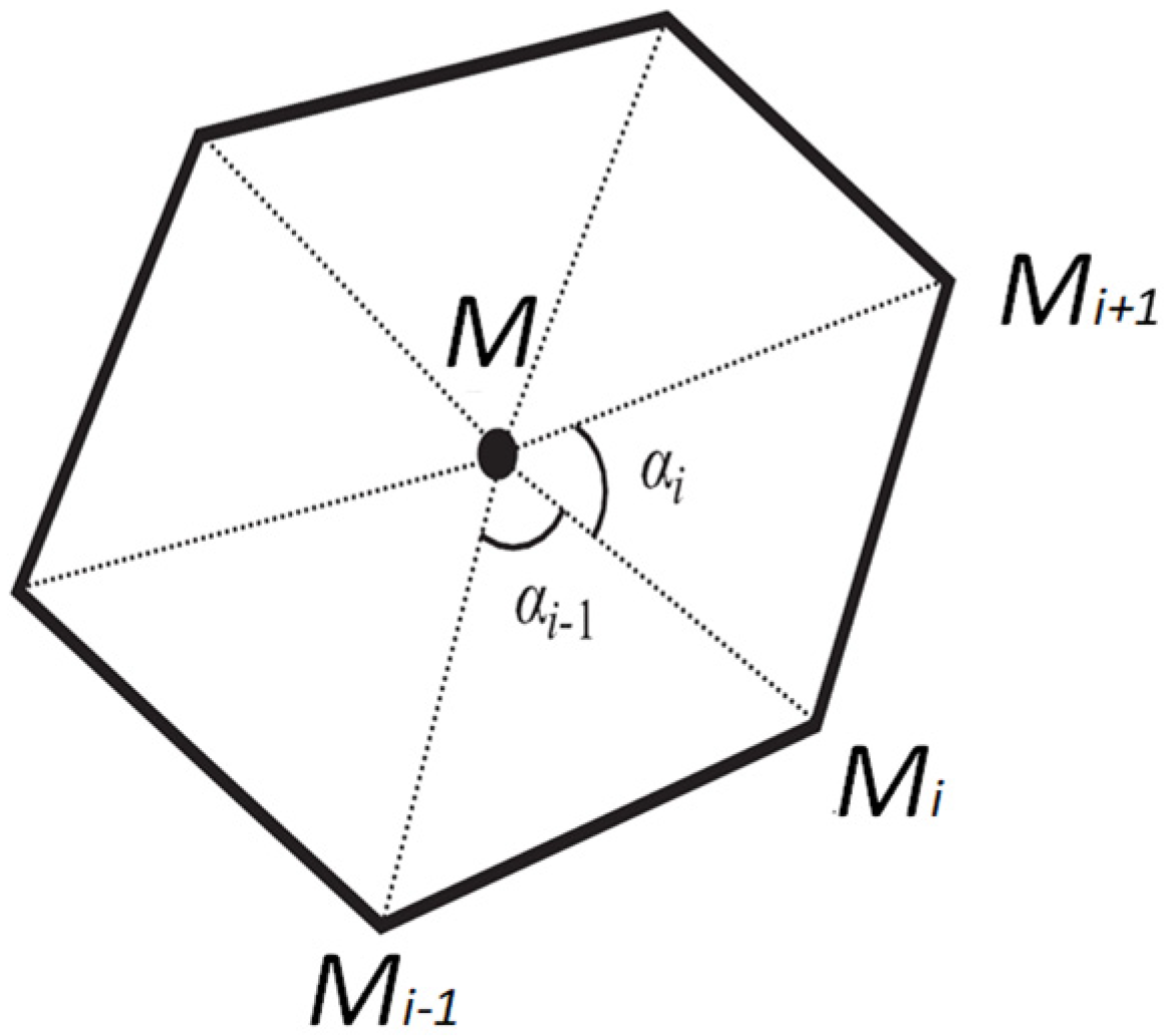
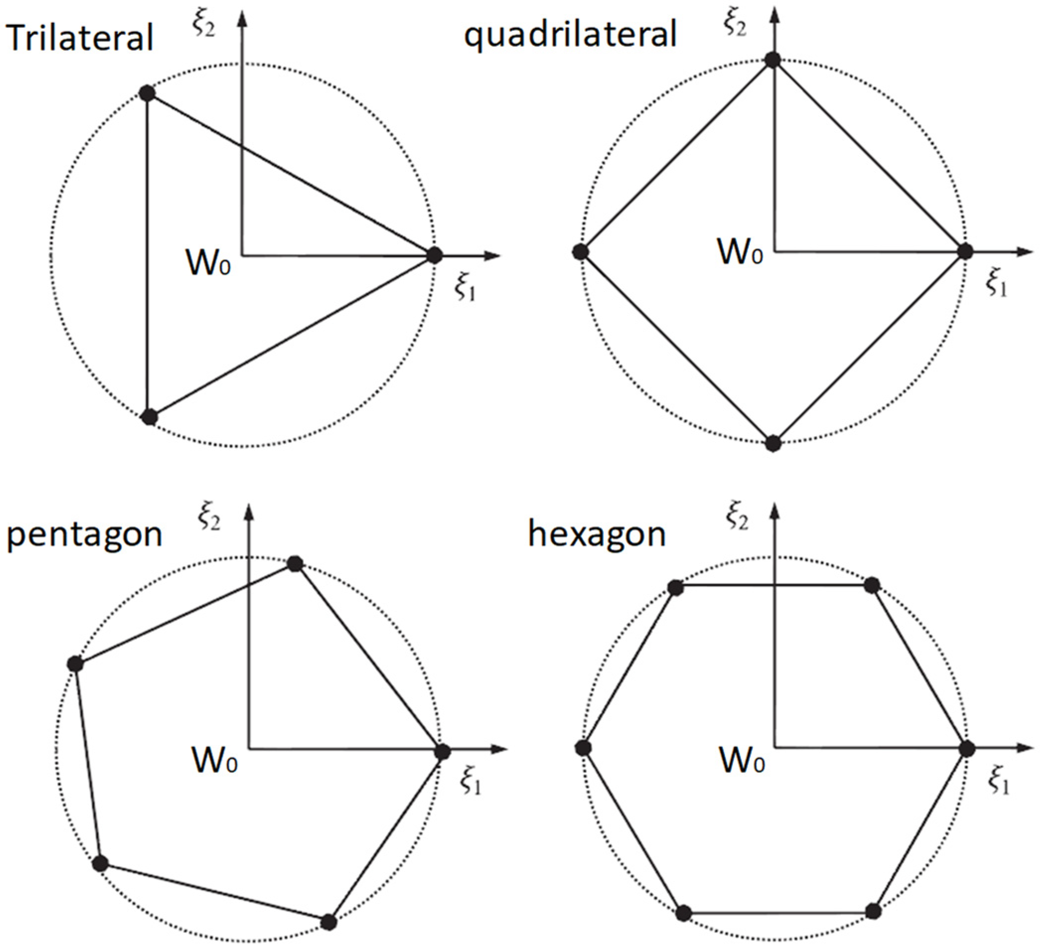
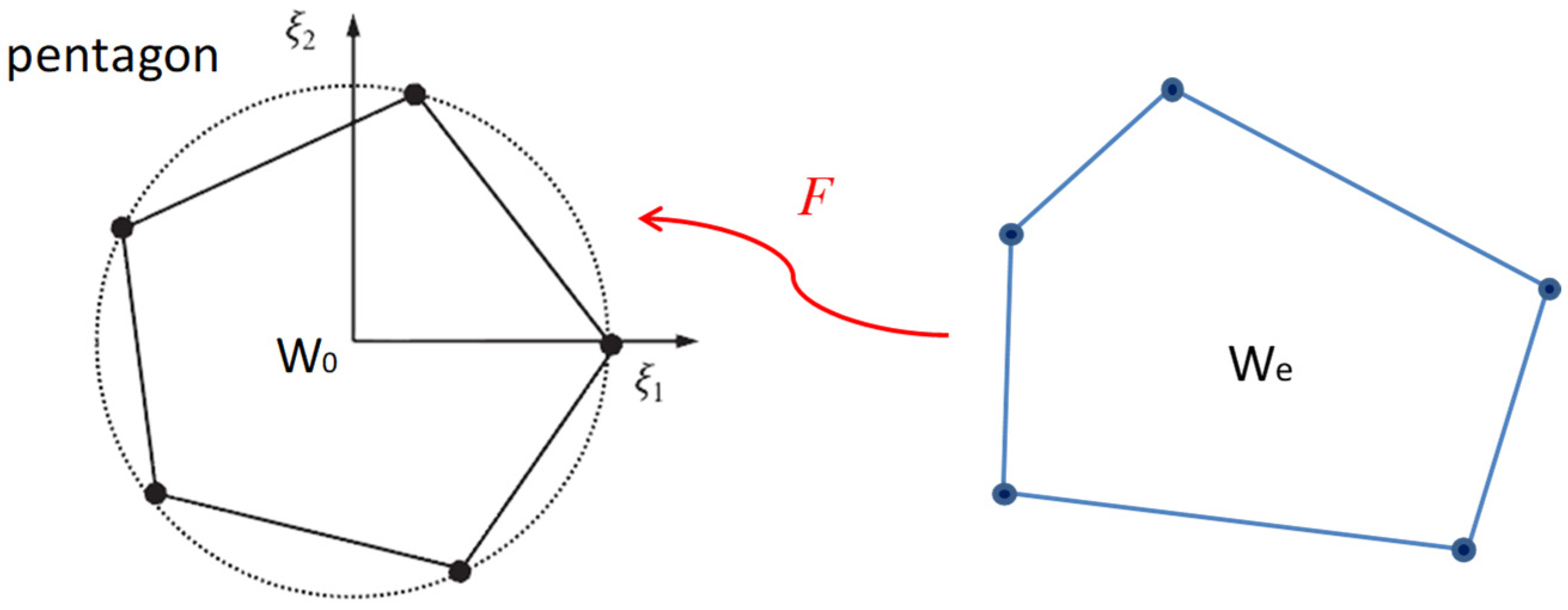
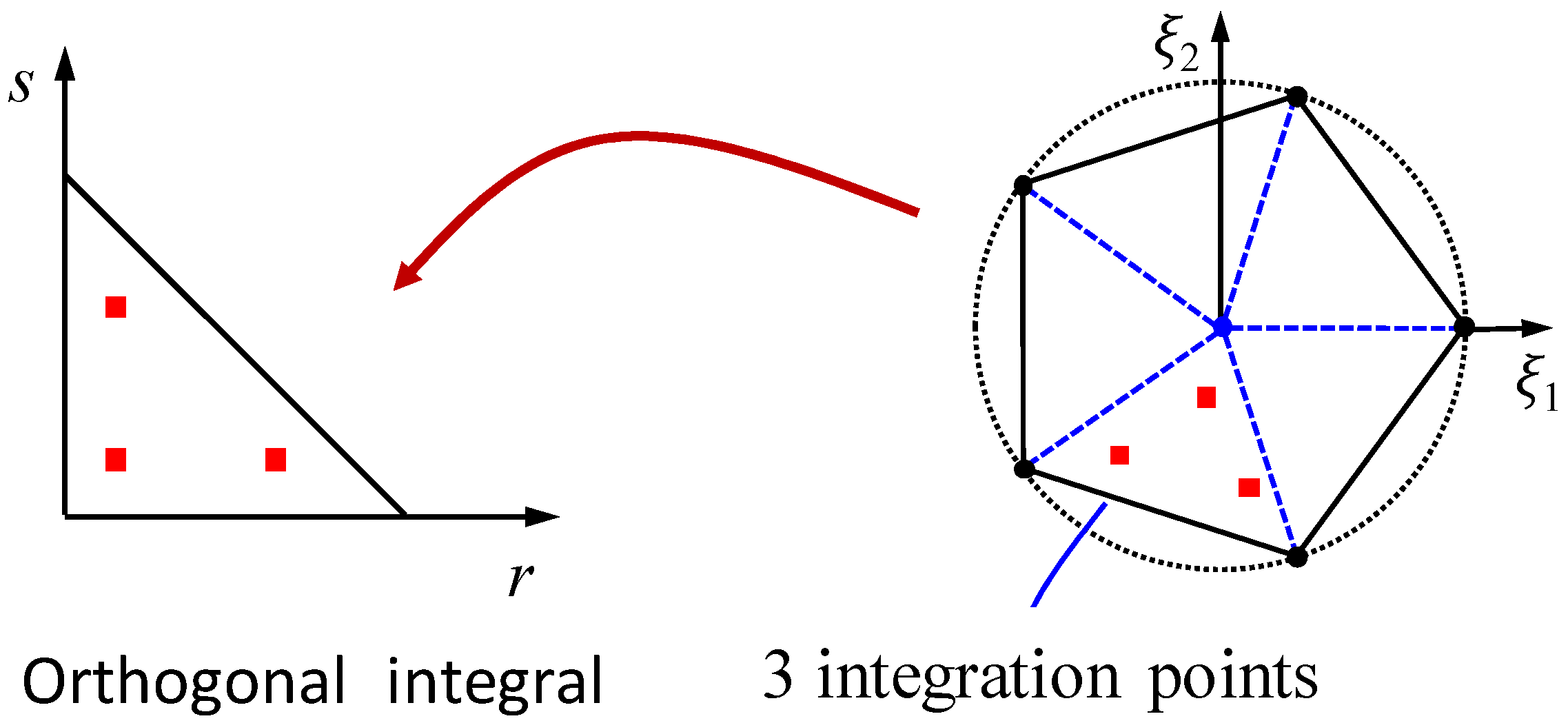
2.2.1. Polygon Mean-Value Shape Function

The mean-value shape function [29,51,52,53] can be used for the interpolating of polygonal elements. The application of the function is straightforward, convenient. and efficient. Initially, this method was employed to analyze and solve FE polygonal elements with an acceptable computational efficiency and accuracy [52]. In this paper, the shape function formulated for general polygonal elements is briefly introduced. A more detailed description can be found in [29,52]. The mean-value coordinate system is shown in Figure 4, and the interpolation function with linear accuracy is expressed as:
N i ( x ) = w i ( x ) j = 1 n w j ( x )
w i ( x ) = t a n ( α i 1 / 2 ) + t a n ( α i / 2 ) x x i
t a n ( α i / 2 ) = s i n   α i 1 + c o s   α i
where w i ( x ) is the weight function, and x x i is the Eulerian distance between points M and Mi (in Figure 4). Point M is selected as the geometric center of the polygon, and n represents the number of vertices on the polygon, that is, the number of edges of the polygon. The interpolation function expressed in Equations (30)–(32) can be used for both convex and concave polygons.
Generally, the shape function is expressed in terms of the Cartesian coordinate system (X1, X2) ∈ We. In order to simplify the integration of the element matrix, it is necessary to construct a conforming approximation of the polygon using mean-value shape functions. Similar to the isoparametric element in FEM, the mean shape function is defined on a standard element in the local coordinate system (ξ1, ξ2) ∈ W0. Four standard elements in the local coordinate system are illustrated as an example in Figure 5: a regular triangle, quadrilateral, pentagon, and hexagon. The vertices of each standard element are placed on the same circumscribed circle with a radius of 1.0, and the geometric center of each element coincides with the center of the circumscribed circle. Therefore, any point in a standard polygon element can be directly connected with each vertex without being occluded. The coordinates of the polygon vertices on the unit circle are (cos 2π/n, sin 2π/n), (cos 4π/n, sin 4π/n), …, and (1, 0), where n is the number of vertices. In this way, the shape function can be defined and used in the local coordinate system as shown in Figure 5, where only four kinds of polygons are shown, and any polygon in the global Cartesian coordinates can be transformed into a standard element using the corresponding local coordinate system through the polygon isoparametric mapping shape function F. An example of the mapping process for a pentagon is illustrated in Figure 6.
After the mapping to the local coordinate system is completed (Figure 7), the standard polygon element is divided into triangular subunits with the center of the circle serving as a common vertex. Then, the element coefficient matrices, such as [E0], [E1], [E2], [M1], and so on, are computed by integrating over the triangular subunits using the standard orthogonal criterion. The triangular subunits in Figure 7 are used only for numerical integration. A detailed discussion of the integration methods can be found in references [29,52].

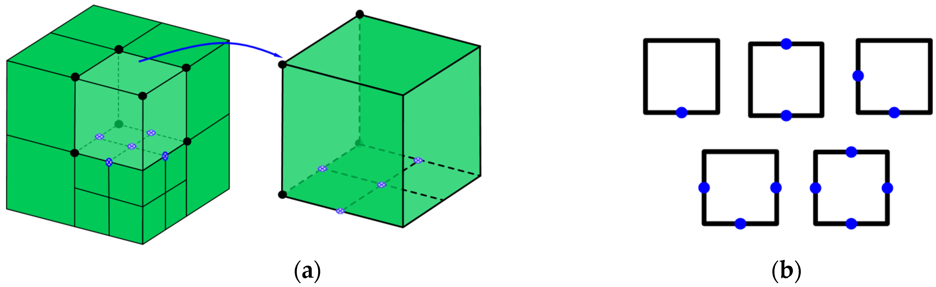
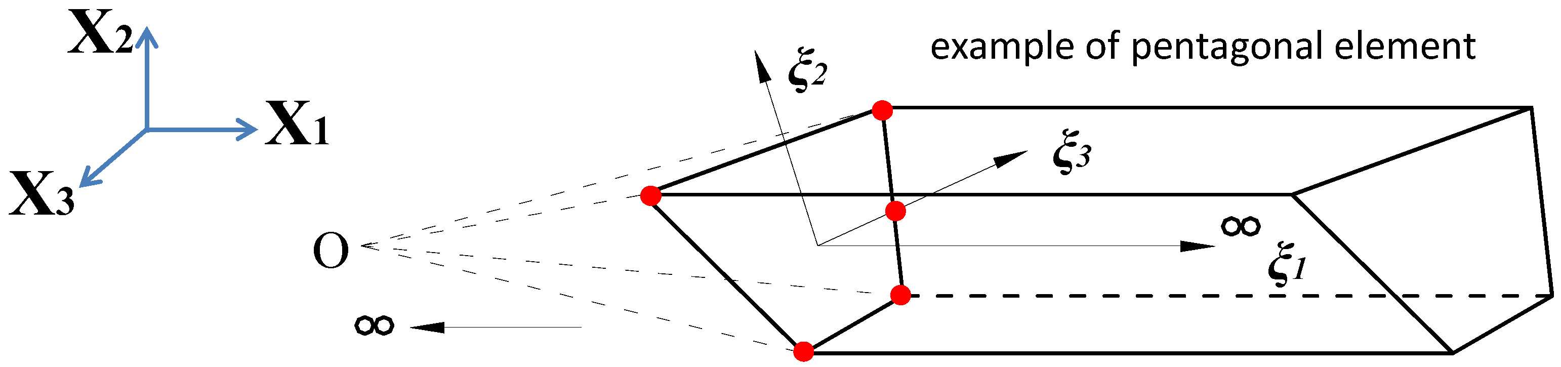
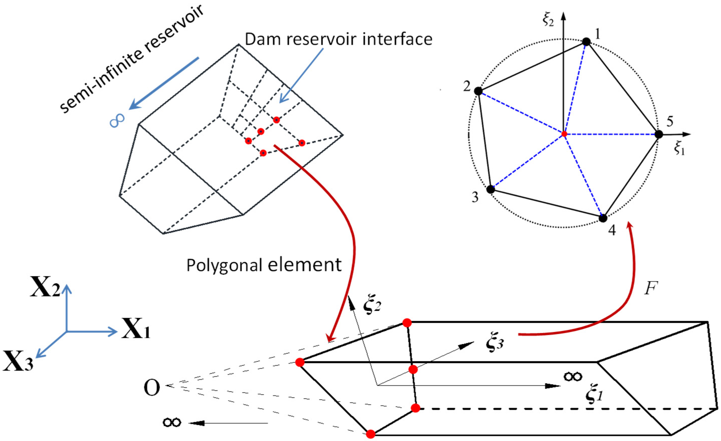
2.2.2. Polyhedral Fluid Elements

As shown in Figure 8, for the dam upstream face with arbitrary convex polygon (triangle, quadrilateral, pentagon, hexagon, heptagon, octagon, etc.) grids, the reservoir model is discretized by the polyhedron SBFEM with polygonal semi-infinite prismatic elements, which are polyhedral fluid elements. A polygonal element (grid) is transformed into a standard unit in the local coordinate system by means of the polygon isoparametric mapping function F. Subsequently, the matrices ([E0], [E1], [E2], [M1], and so on) for the polyhedral element are integrated and calculated. In the end, the total matrices of all reservoir elements are integrated, and the hydrodynamic pressure can be directly solved as mentioned in Section 2.1.

3. A Nonlinear Dynamic Coupling Method for Cross-Scale Dam-Reservoir Systems Based on the Polyhedron SBFEM

The establishment of the dynamic coupling method consists of two main phases: the procedure implementation for the hydrodynamic pressure computation method and analysis implementation for the coupling calculation equation of dam-reservoir systems.

3.1. Polyhedron SBFEM Procedure for Fluid

The polygonal semi-infinite prismatic fluid elements (i.e., polyhedral elements) are implemented based on the Windows programs GEODYNA [54], which was developed by the fifth author using object-oriented programming in Visual C++. Multicore parallel technology of the CPU coupled with the GPU is realized in the GEODYNA program, by which the computational capacity of solving a large-scale elasto-plastic analysis with millions of DOFs is provided. The GEODYNA program has been applied to the dynamic analysis of nonlinear structures [26,27,28,45,46,48,55,56,57,58,59,60,61,62].

3.2. Nonlinear Dynamic Coupling Method for Cross-Scale CFRD-Reservoir Systems

The nonlinear dam, including the foundation, is modeled by the polyhedron SBFEM with cross-scale mesh, and the reservoir is modeled by the polyhedron SBFEM for fluid. In this way, the equation for the dynamic coupling analysis between the CFRD and reservoir can be expressed as follows:
[ M s ] { u ¨ r ( t ) } + [ C s ] { u ˙ r ( t ) } + [ K s ] { u r ( t ) } = [ M s ] { u ¨ g ( t ) } ( 1 / ρ ) [ L 1 ] T [ M 1 ] T { p ( ξ = 0 ) }
where [Ms], [Cs], and [Ks] are, respectively, the mass, damping, and stiffness matrices of the dam and foundation. {ür(t)}, { u ˙ r ( t ) } , and {ur(t)} are, respectively, the relative acceleration, velocity, and displacement. {üg(t)} is the input earthquake acceleration from bedrock. [L1] is the conversion matrix between global coordinates and the local coordinates of the dam surface.
Substituting Equation (27) into Equation (33), the dynamic fluid–solid coupling analysis equations are derived further as:
( [ M s ] + [ M p ] ) { u ¨ r ( t ) } + [ C s ] { u ˙ r ( t ) } + [ K s ] { u r ( t ) } = ( [ M s ] + [ M p ] ) { u ¨ g ( t ) }
[ M p ] = ( 1 / ρ ) [ L 1 ] T [ M 1 ] T { [ Φ 12 ] [ Φ 22 ] 1 [ M 1 ] [ L 1 ] + ( [ Φ 12 ] [ Φ 22 ] 1 [ B 1 ] [ B 2 ] ) ρ [ C 0 ] [ L 2 ] }
[ L 1 ] { u ¨ g ( t ) + u ¨ r ( t ) } = { u ¨ n } ,                   [ L 2 ] { u ¨ g ( t ) + u ¨ r ( t ) } = { ν ¨ n }
where [Mp] is the additional mass matrix of hydrodynamic pressure. [L2] is the conversion matrix between global coordinates and the local coordinates of the river valley surrounding the reservoir.
As shown in Equation (34), the dynamic interaction analysis between the dam and the reservoir water can be realized directly by superimposing the additional mass matrix of the hydrodynamic pressure [Mp] into the mass matrix of the dam [Ms]. Then, a strong coupling method for a nonlinear cross-scale dam-reservoir system is established based on the polyhedron SBFEM.

4. Numerical Examples of Rigid Dams and River Valley

The following numerical examples of rigid dams, which have analytical solutions, have been selected for analysis and validation of the accuracy of the presented method for hydrodynamic pressure. The computed hydrodynamic pressure distribution due to earthquakes in the upstream–downstream, vertical, and dam axial directions have been compared with analytical solutions [63,64,65,66].

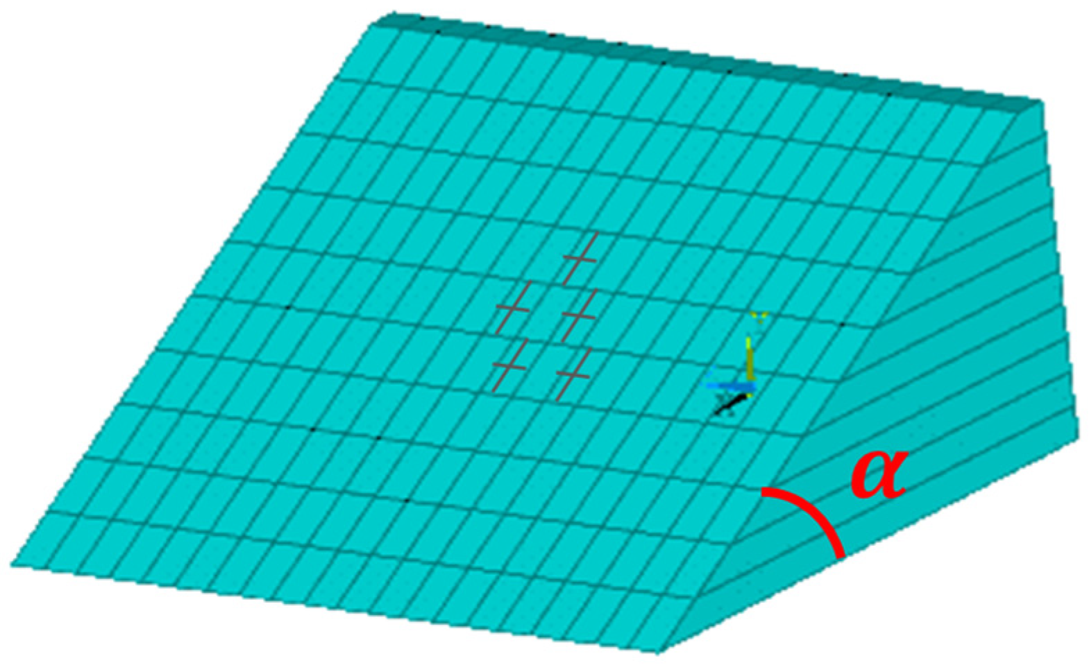
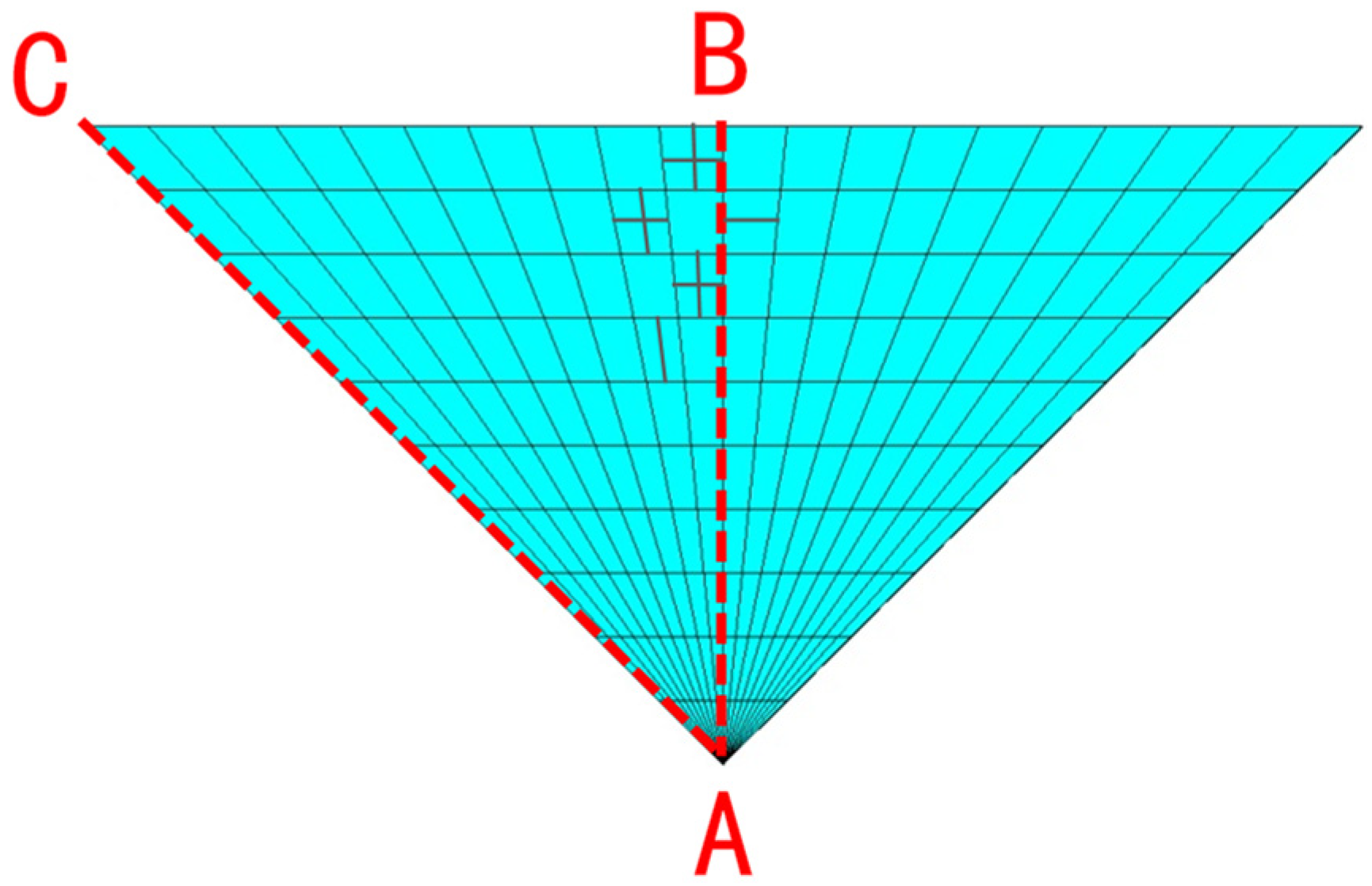
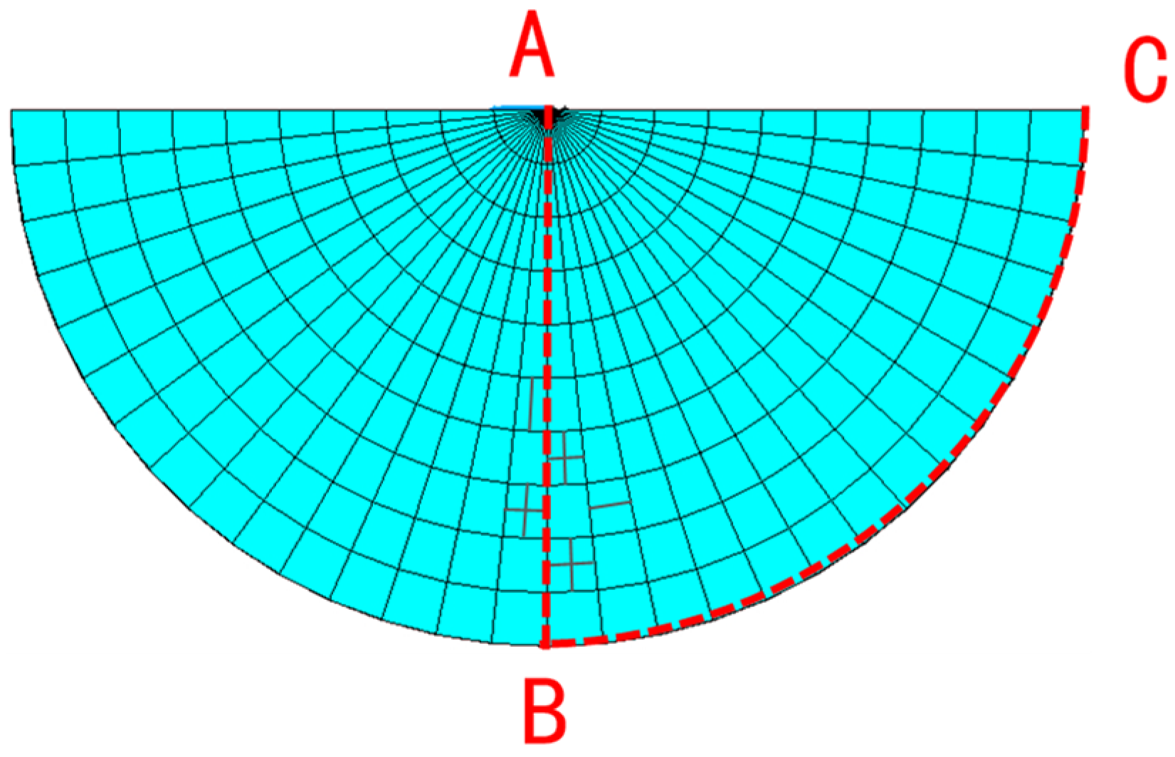
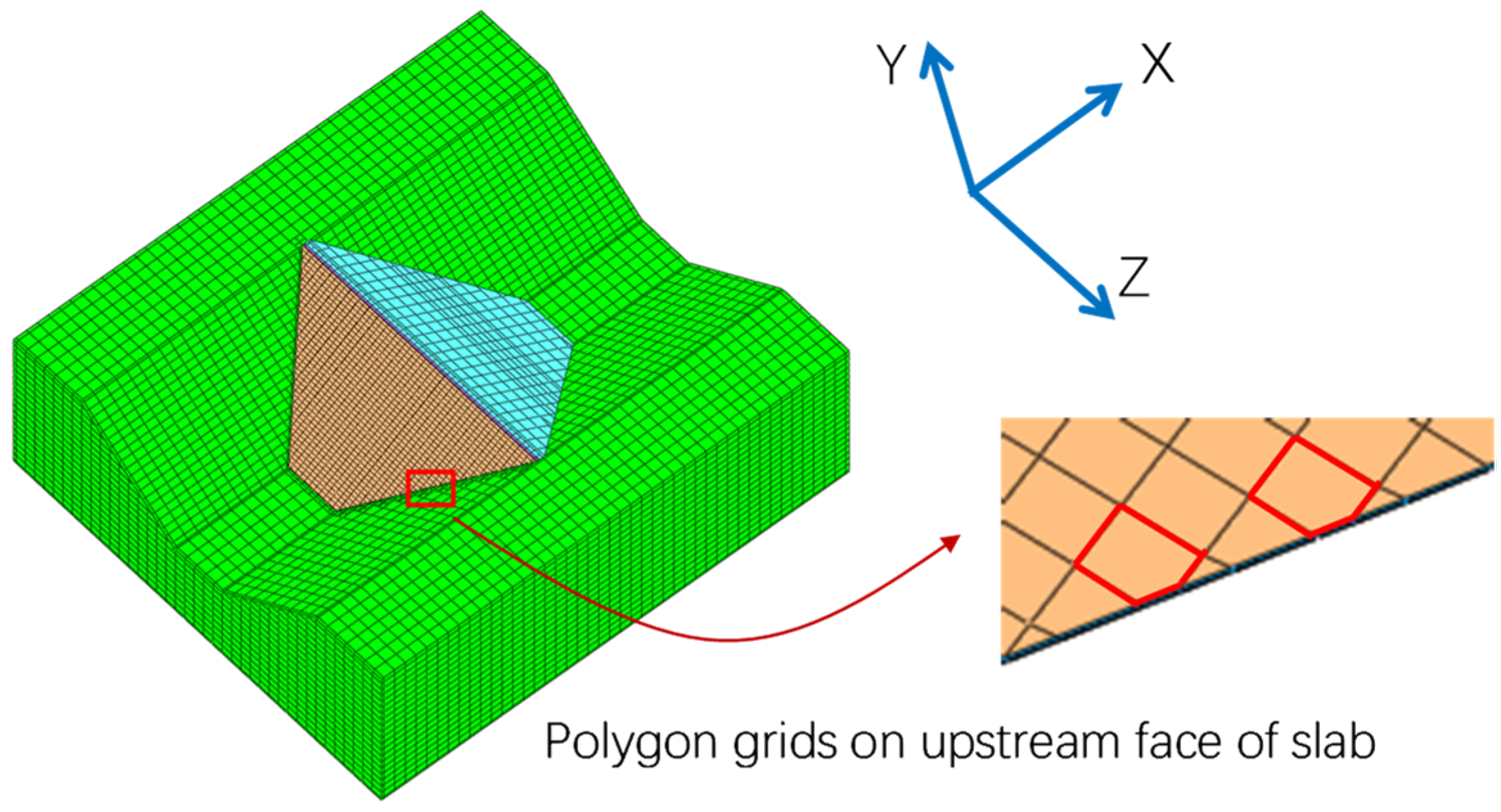
4.1. Dams with Polygonal Mesh on Upstream Face

The first group of examples are shown in Figure 9. An inclined dam face in a rectangular valley with a height and width of 180 m was selected. The water depth of the reservoir was 180 m (i.e., full reservoir condition), and the dam upstream face inclination angles were 30°, 45°, and 60°, respectively.
The second group of examples are shown in Figure 10. A 120-m high vertical dam face in an isosceles right triangular valley was selected. The water depth of the reservoir was 120 m (i.e., full reservoir condition).
The third group of examples are shown in Figure 11. A vertical dam face in the semi-circular valley with a radius of 100 m was selected. The water depth of the reservoir was 100 m (i.e., full reservoir condition).
The 2D dam upstream face meshes of the above three groups of calculation examples, which are plotted in Figure 9, Figure 10 and Figure 11, were just used as the SBFEM meshes of the reservoir water. Furthermore it can be observed that the dam upstream faces contained pentagon, hexagon, heptagon, and octagon polygon grids, which often appear when polyhedron elements based on the polyhedron SBFEM are used to model dams. The peak acceleration of seismic excitation in different directions is expressed as a, the density of water is expressed as ρ, and the water depth is expressed as H.

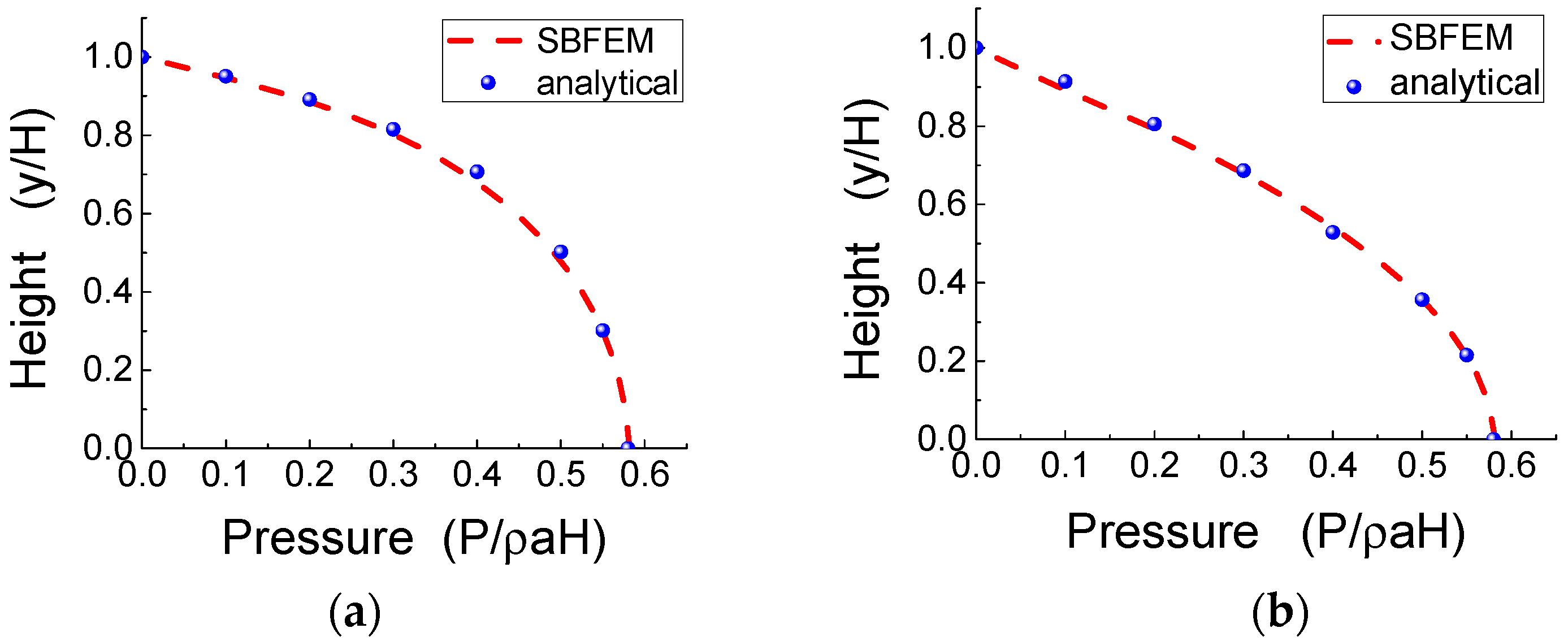
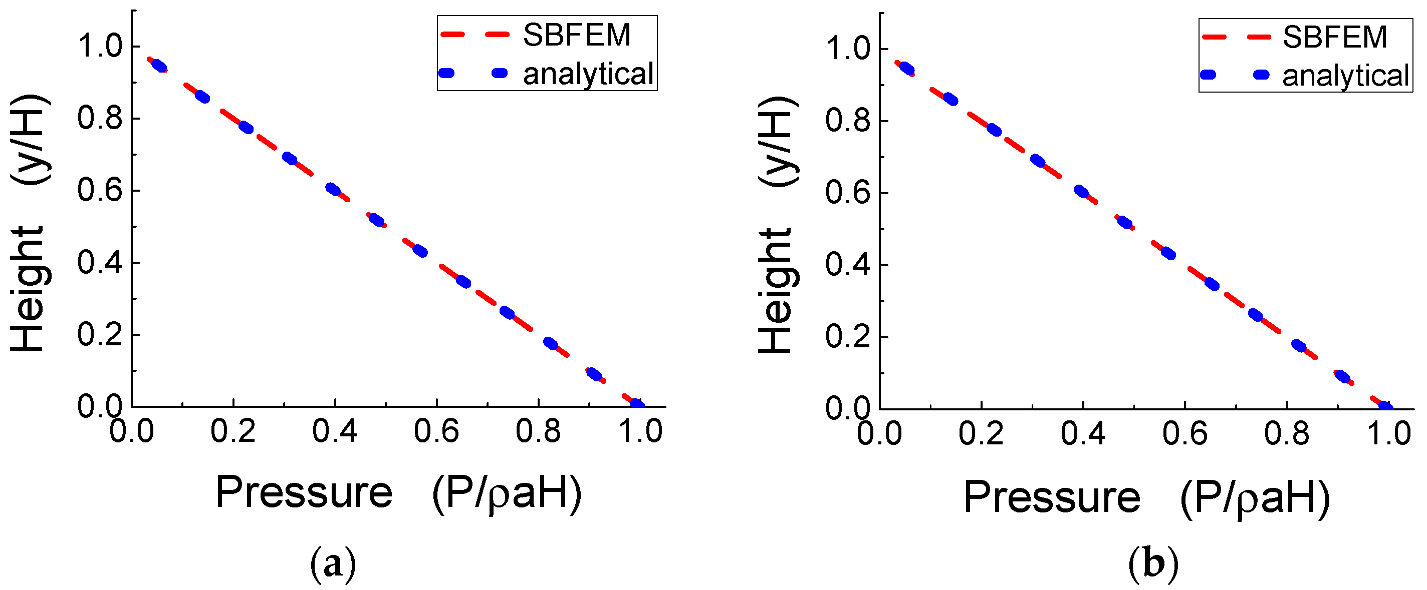
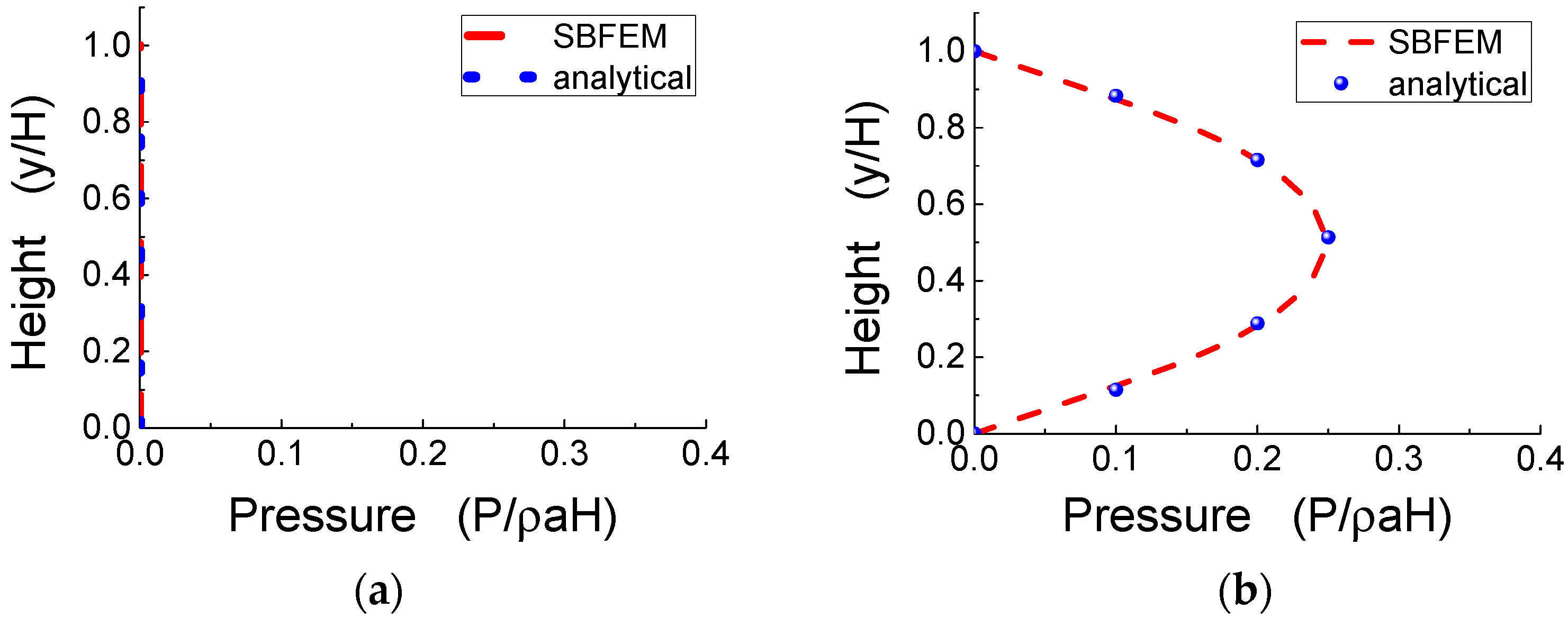
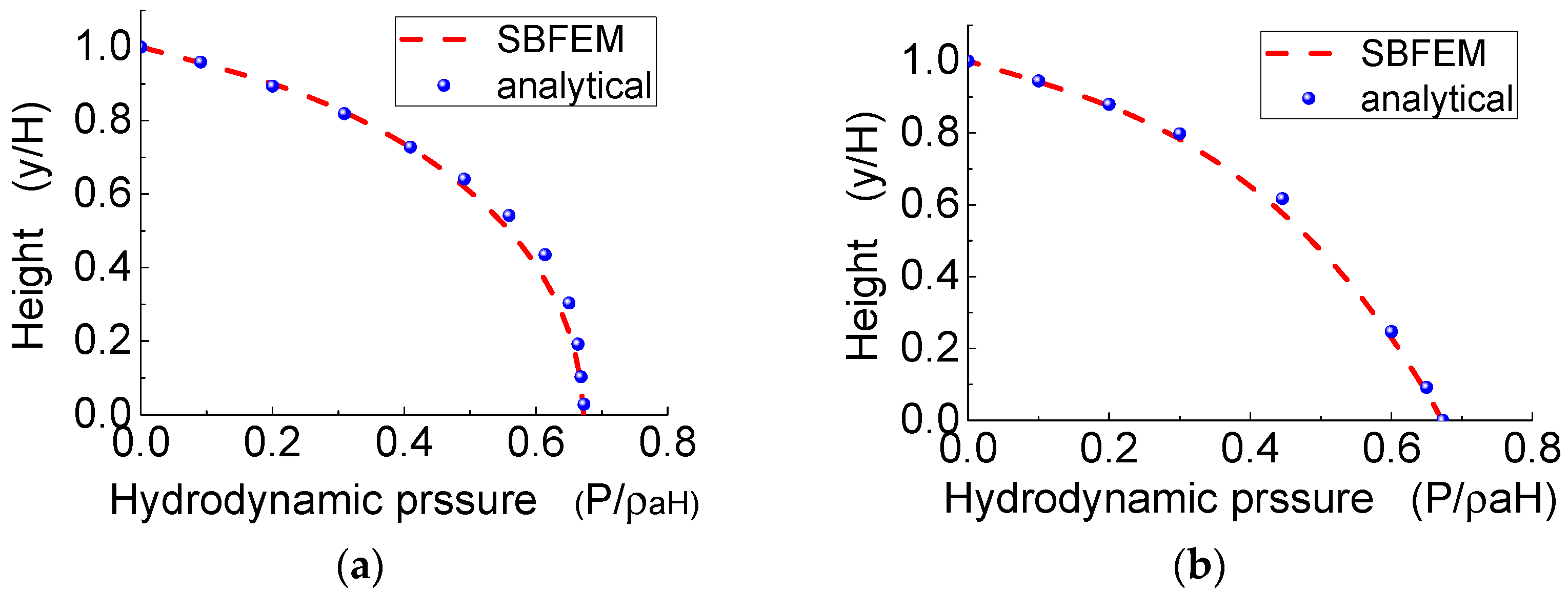
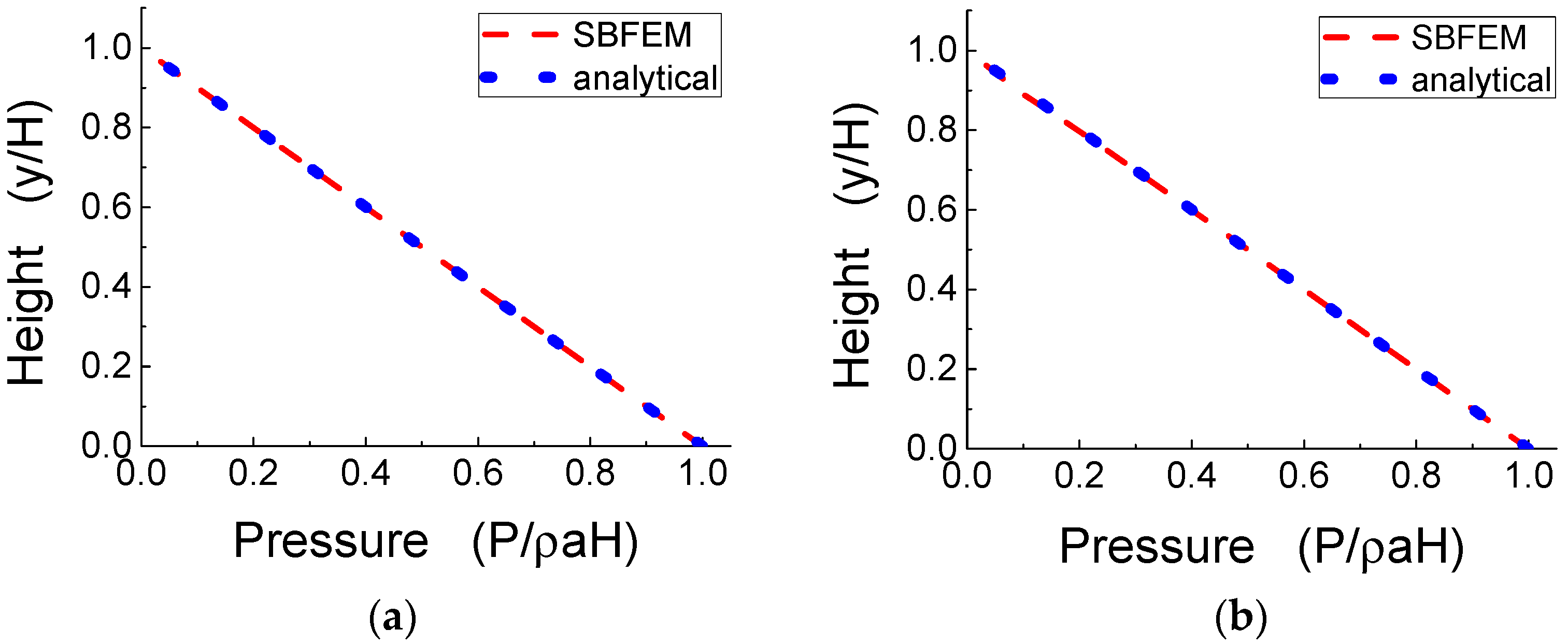
4.2. Results and Discussion

Figure 12 shows the distribution of hydrodynamic pressure for the condition in which the dam face is inclined in a rectangular valley. Figure 13, Figure 14 and Figure 15 provide the results for the case in the triangular valley. Figure 16, Figure 17 and Figure 18 show the distribution of hydrodynamic pressure on the dam face in the semi-circular valley. From the above figures (Figure 12, Figure 13, Figure 14, Figure 15, Figure 16, Figure 17 and Figure 18), it can be seen that the proposed hydrodynamic pressure calculation method based on polyhedron SBFEM could precisely compute the hydrodynamic pressure on the dam face induced by an earthquake in different directions and could accurately consider factors such as the inclination of the dam face and the complex shape of the river valley.
Moreover, the proposed method has a high efficiency, because only 2D discretization was required to simulate the 3D semi-infinite reservoir water. Therefore, the proposed hydrodynamic pressure method can serve as a convenient analysis tool for further establishing a dynamic coupling analysis method for the dam–reservoir systems when polyhedral solid elements are utilized to build cross-scale models of dams.

5. Dynamic Coupling Analysis of Nonlinear Cross-Scale CFRD and Reservoir Systems

With the polyhedron SBFEM for solid and fluid being used to discretize the CFRD and reservoir, the elasto-plastic cross-scale dynamic coupling analysis was conducted to investigate the effect of hydrodynamic pressure on the dynamic response of CFRD. The results of the CFRD under static loading, including the filling and impounding processes, were introduced into the seismic analysis as the initial state.

5.1. Cross-Scale Model of the CFRD and Reservoir

The 3D polyhedron cross-scale mesh of a 100-m high dam and rock foundation is shown in Figure 19. The concrete slab grid was dense, and the rockfill grid was relatively coarse. In order to achieve a rapid cross-scale meshing from the slab to the rockfill, some polyhedral meshes appeared on upstream face of the slab inevitably. The upstream slope of the dam was 1 V:1.4 H, and the downstream slope was 1 V:1.6 H. The valley was a prismatic valley with a trapezoidal section with a bottom width of 70 m and a slope ratio of 1 V:1 H on both banks. The mesh of the dam and foundation had a total of 39,145 elements, of which the slab and interface both had 1272 elements. The slab and rockfill were simulated by polyhedral elements based on SBFEM [27]. Furthermore, the interface between the slab and cushion, slab joints, and peripheral joints were simulated by polygonal Goodman elements [27]. The displacement of the bottom boundary of the massless bedrock in the three directions of the global coordinate system was constrained, and the normal displacement of the lateral boundary was constrained.
The depth of the reservoir in front of the dam was 90 m. When the proposed method was used to calculate the hydrodynamic pressure, the mesh of the semi-infinite reservoir water could be directly generated using the 2D polygonal grid on the upstream face of the concrete slab, as indicated in Figure 3. Therefore, the pre-processing of the reservoir model was simplified to a large extent, and the overall analysis efficiency was improved.

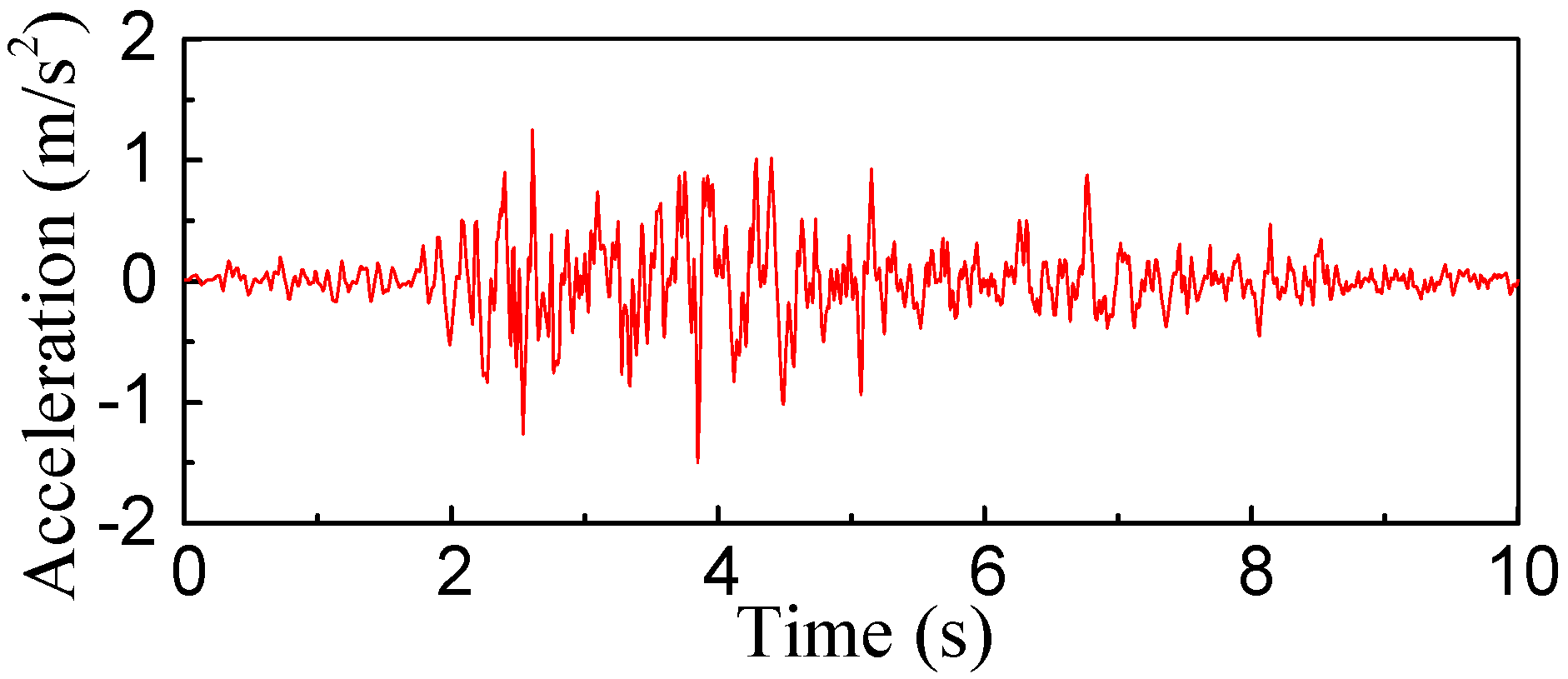
5.2. Material Parameters, Damping Methods, and Ground Motion

A linear elastic model was adopted for both the concrete face slab (density ρ = 2.40 g/cm3, elasticity modulus E = 25 GPa, Poisson’s ratios ν = 0.167) and bedrock (density ρ = 2.50 g/cm3, elasticity modulus E = 20 GPa, Poisson’s ratios ν = 0.2). An improved P–Z generalized plastic model was used for rockfills [59,67], of which the 17 material parameters were calibrated by the results of the triaxial tests and listed in the Table 1. Furthermore, an ideal elasto-plastic model was used to model the interface between the face slab and rockfills, of which the parameters are listed in Table 2. The compression stiffness of the slab and peripheral joints was 25,000 MPa/m, and the shear stiffness was 1 MPa/m. The Rayleigh damping method was employed for the various material and mechanical models of the CFRD.
Seismic waves were the input in the upstream–downstream direction for the dynamic coupling analysis. The time history of the seismic acceleration measured from a real earthquake in Figure 20 was selected. The peak ground acceleration (PGA) was 1.5 m/s2. The results of the two conditions, which were considering the hydrodynamic pressure based on the polyhedron SBFEM condition and neglecting the hydrodynamic pressure condition, are compared and analyzed in the following section.

5.3. Results and Discussion

Due to the existence of reservoir water in front of the dam, the dam would definitely be affected by hydrodynamic pressure under an earthquake condition. The proposed hydrodynamic pressure calculation method based on the polyhedron SBFEM, which was proved to be accurate in Section 4.2, is adequate for analyzing the effect of hydrodynamic pressure on the dynamic response of the rockfill in CFRD. For the condition of ignoring hydrodynamic pressure, the additional mass matrix of hydrodynamic pressure [Mp] in Equation (34) was a null matrix, which meant that errors would occur because it was inconsistent with the actual situation. When calculating the error of the dynamic response of rockfill and concrete face slabs in the CFRD caused by ignoring the hydrodynamic pressure, the results under the condition of considering the hydrodynamic pressure were used as a standard. The compressive stress of the face slabs was positive.

5.3.1. Rockfill

Table 3 lists the maximum absolute values of the dynamic acceleration and displacement for the rockfill under an earthquake and the corresponding errors caused by neglecting the hydrodynamic pressure. Compared to the results from the condition of calculating hydrodynamic pressure by the polyhedron SBFEM, the maximum errors of acceleration and displacement were 15.4% and 12.7%, respectively, when the hydrodynamic pressure was ignored. Figure 21 and Figure 22 show the maximum distribution of the dynamic acceleration along the upstream–downstream direction (ax) and the dynamic displacement along the vertical direction (dy). As can be seen from Figure 21 and Figure 22 and Table 3, the distribution rules of the dynamic response for the rockfill were consistent under the two conditions of hydrodynamic pressure, but the differences of the maximum value and the corresponding size of the area with a large response were obvious. The dynamic acceleration and displacement of the rockfill were smaller when hydrodynamic pressure was considered.
In summary, when the hydrodynamic pressure is ignored, the dynamic acceleration and displacement response of a rockfill may be overestimated obviously, which is not conducive to the accurate and reasonable safety evaluation of CFRD under an earthquake.

5.3.2. Concrete Face Slabs

Table 4 lists the maximum dynamic concrete face slabs’ stresses under the two hydrodynamic pressure conditions and the relative errors of stresses caused by neglecting the hydrodynamic pressure. Compared with the results by the polyhedron SBFEM, the maximum errors in the dynamic face slabs’ stresses along the slope direction and the dam axial direction for neglecting the hydrodynamic pressure condition were 22.5% and 24.9%, respectively. It can be observed from Table 4 that the errors of the maximum face slabs’ stress along the slope direction and the dam axial direction caused by neglecting the hydrodynamic pressure were obvious, and the hydrodynamic pressure cannot be ignored in the dynamic stress analysis of face slabs. Figure 23 and Figure 24 plot the distributions of the maximum dynamic tensile stress in face slabs along the slope direction and compressive stresses in face slabs along the dam axial direction. Figure 23 and Figure 24 show that the distributions of the extreme stresses along the slope direction and the dam axial direction for both hydrodynamic pressure conditions were similar, but the extent of the high stress regions was significantly different.
As can be concluded from the above Figure 23 and Figure 24 and Table 4, for a high CFRD located in front of a reservoir, the hydrodynamic pressure has a big influence on the dynamic face slabs’ stresses along the slope direction and the dam axial direction. It is possible to significantly overestimate or underestimate the dynamic concrete face slabs’ stress when hydrodynamic pressure is ignored in the seismic analysis of a CFRD.

6. Conclusions

In this paper, polyhedral scaled boundary finite elements of fluid were constructed using the polygon mean-value shape function to compute the hydrodynamic pressure of a reservoir on a dam, which is applicable for not only a polygon mesh but also triangular and quadrilateral meshes on the upstream face of a dam. Moreover, a nonlinear cross-scale dynamic analysis of CFRD-reservoir systems under a seismic condition was carried out, and the effect of hydrodynamic pressure on the dynamic response of a rockfill in CFRD was investigated. The following primary conclusions are summarized:
(1)
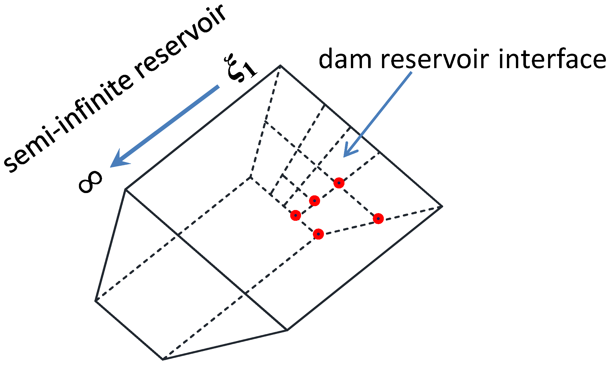
A 3D hydrodynamic pressure calculation method based on the polyhedron SBFEM was proposed, in which the reservoir in front of a dam was simulated with polygonal semi-infinite prismatic fluid elements. The pre-processing of the reservoir model was simplified to a large extent, as the 3D mesh of the reservoir could be generated automatically from the 2D grid of the upstream face of dam. A high efficiency was achieved also by reducing the one-dimensional discretization. The proposed method has a high accuracy and provides a convenient numerical tool for a dynamic coupling analysis of a dam–reservoir system, when the cross-scale dam is modeled by the polyhedron SBFEM.
(2)
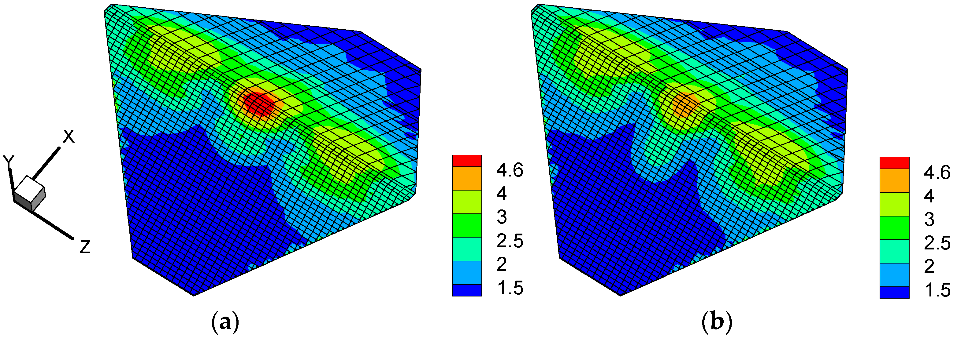
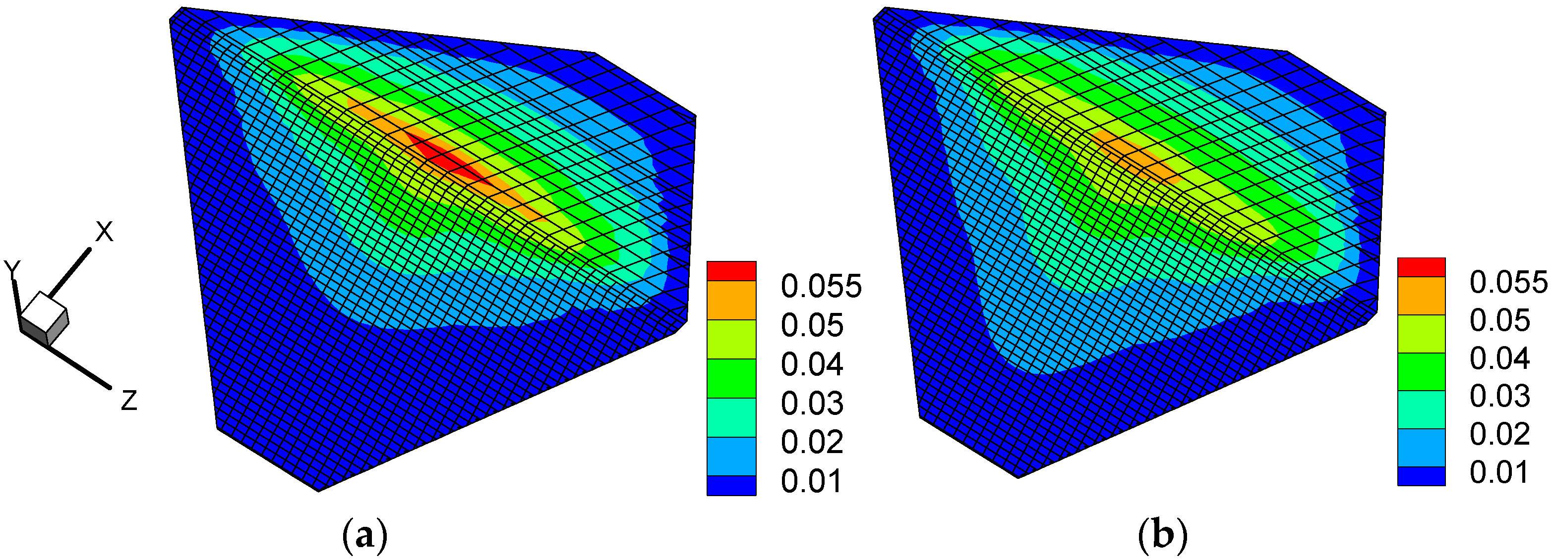
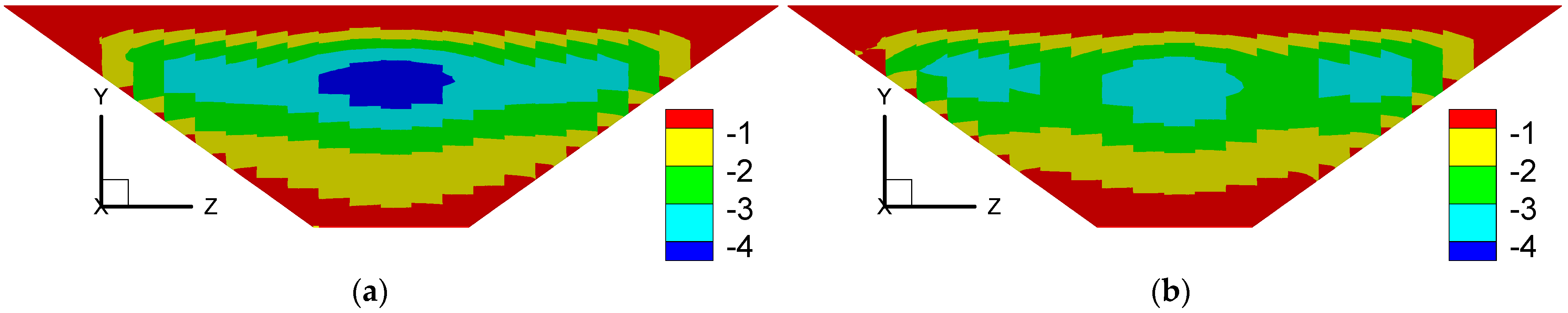
With an elastic–plastic CFRD being simulated by the polyhedron SBFEM and the hydrodynamic pressure of the reservoir being computed by the proposed polyhedron SBFEM for fluid, respectively, a nonlinear dynamic coupling method for cross-scale CFRD-reservoir systems based on the polyhedron SBFEM was developed. The results of a further numerical analysis showed that neglecting hydrodynamic pressure may produce obvious errors and lead to overestimation of the dynamic acceleration and displacement response of the rockfill, which is not conducive to an accurate and reasonable safety evaluation of a CFRD under an earthquake. Moreover, the hydrodynamic pressure had a big influence on the dynamic face slabs’ stresses, and the hydrodynamic pressure cannot be ignored in the dynamic stress analysis of face slabs.
The hydrodynamic pressure calculation method proposed in this paper can also be applied to a dynamic linear or nonlinear analysis of cross-scale arch dams or gravity dams simulated by the polyhedron SBFEM for seismic safety evaluation.

Author Contributions

Conceptualization, H.X. and D.Z.; methodology, H.X. and J.X.; software, H.X. and K.C.; validation, H.X. and D.Y.; resources, H.X., K.C. and D.Z.; writing—original draft preparation, J.X. and H.X.; writing—review and editing, D.Y. and K.C.; supervision, J.X., H.X., D.Y., K.C. and D.Z. All authors have read and agreed to the published version of the manuscript.

Funding

This work was supported by the Project funded by the China Postdoctoral Science Foundation (2021M690998) and the National Natural Science Foundation of China (Grant Nos. U1965206, 52192674).

Institutional Review Board Statement

Not applicable.

Informed Consent Statement

Not applicable.

Data Availability Statement

Not applicable.

Conflicts of Interest

The authors declare no conflict of interest.

Nomenclature

2Laplacian operator
pHydrodynamic pressure
ρFluid density
ünNormal accelerations of the dam–reservoir interface
ϋnNormal accelerations of the river –valley interface
[ N ( ξ 2 , ξ 3 ) ] Polygon mean-value shape function
[J]Jacobian matrix
wweight function
[E0], [E1], [E2], [C0], [M1]Coefficient matrices
{ q ( ξ 1 ) } Nodal force
[Z]Hamilton coefficient matrix
[Λ]Eigenvalue matrix
[Φ]Eigenvector matrix
[A]The inverse of eigenvector matrix [Φ]
N i ( x ) Interpolation function in mean-value coordinate system
w i ( x ) Weight function of mean-value coordinate system
x x i Eulerian distance between points
WeCartesian coordinate system
W0Local coordinate system
[Ms], [Cs], [Ks]Mass, damping and stiffness matrices
{ür(t)}, { u ˙ r ( t ) } , {ur(t)}Relative acceleration, velocity, and displacement
{üg(t)}Input earthquake acceleration
[Mp]Additional mass matrix of hydrodynamic pressure
[L1], [L2]Conversion matrix
(x1, x2, x3)Global coordinates
(ξ1, ξ2, ξ3)Local scaled boundary coordinates
EElasticity modulus
ν Poisson’s ratios
SBFEMScaled boundary finite element method
CFRDConcrete faced rockfill dam
3DThree-dimensional
2DTwo-dimensional
DOFDegrees of freedom
FEMFinite element method
BEMBoundary element method
PSBFEMPolyhedron SBFEM
PGAPeak ground acceleration

References

  1. Song, C.M. The Scaled Boundary Finite Element Method: Introduction to Theory and Implementation; John Wiley & Sons Ltd.: Hoboken, NJ, USA, 2018. [Google Scholar]
  2. Wolf, J.P.; Song, C. The scaled boundary finite-element method—A primer: Derivations. Comput. Struct. 2000, 78, 191–210. [Google Scholar] [CrossRef]
  3. Ooi, E.T.; Song, C.M.; Natarajan, S. A scaled boundary finite element formulation with bubble functions for elasto-static analyses of functionally graded materials. Comput. Mech. 2017, 60, 943–967. [Google Scholar] [CrossRef]
  4. Xue, B.; Lin, G.; Hu, Z. Scaled boundary isogeometric analysis for electrostatic problems. Eng. Anal. Bound. Elem. 2017, 85, 20–29. [Google Scholar] [CrossRef]
  5. Zhang, X.; Wegner, J.L.; Haddow, J.B. Three-dimensional dynamic soil-structure interaction analysis in the time domain. Earthq. Eng. Struct. Dyn. 1999, 28, 1501–1524. [Google Scholar] [CrossRef]
  6. Wegner, J.L.; Zhang, X. Free-vibration analysis of a three-dimensional soil-structure system. Earthq. Eng. Struct. Dyn. 2001, 30, 43–57. [Google Scholar] [CrossRef]
  7. Genes, M.C.; Aslmand, M.; Kani, M. Efficient Dynamic Analysis of Foundation Via a Coupled Axisymmetric SBFEM-3D FEM. Teknik Dergi 2019, 30, 9327–9352. [Google Scholar] [CrossRef]
  8. Schauer, M.; Rios Rodriguez, G. A coupled FEM-SBFEM approach for soil-structure-interaction analysis using non-matching meshes at the near-field far-field interface. Soil Dyn. Earthq. Eng. 2019, 121, 466–479. [Google Scholar] [CrossRef]
  9. Yaseri, A. 2.5D coupled FEM-SBFEM analysis of ground vibrations induced by train movement. Soil Dyn. Earthq. Eng. 2017, 104, 307–318. [Google Scholar] [CrossRef]
  10. Chen, D.; Dai, S. Dynamic fracture analysis of the soil-structure interaction system using the scaled boundary finite element method. Eng. Anal. Bound. Elem. 2017, 77, 26–35. [Google Scholar] [CrossRef]
  11. Song, C.; Wolf, J.P. Semi-analytical representation of stress singularities as occurring in cracks in anisotropic multi-materials with the scaled boundary finite-element method. Comput. Struct. 2002, 80, 183–197. [Google Scholar] [CrossRef]
  12. Zhang, P.; Du, C.; Tian, X.; Jiang, S. A scaled boundary finite element method for modelling crack face contact problems. Comput. Methods Appl. Mech. Eng. 2018, 328, 431–451. [Google Scholar] [CrossRef]
  13. Yao, F.; Yang, Z.J.; Hu, Y.J. An SBFEM-Based Model for Hydraulic Fracturing in Quasi-Brittle Materials. Acta Mech. Solida Sin. 2018, 31, 416–432. [Google Scholar] [CrossRef]
  14. Adak, D.; Pramod, A.; Ooi, E.T.; Natarajan, S. A combined virtual element method and the scaled boundary finite element method for linear elastic fracture mechanics. Eng. Anal. Bound. Elem. 2020, 113, 9–16. [Google Scholar] [CrossRef]
  15. Chen, K.; Zou, D.; Tang, H.; Liu, J.; Zhuo, Y. Scaled boundary polygon formula for Cosserat continuum and its verification. Eng. Anal. Bound. Elem. 2021, 126, 136–150. [Google Scholar] [CrossRef]
  16. Qu, Y.; Zou, D.; Kong, X.; Yu, X.; Chen, K. Seismic cracking evolution for anti-seepage face slabs in concrete faced rockfill dams based on cohesive zone model in explicit SBFEM-FEM frame. Soil Dyn. Earthq. Eng. 2020, 133, 106106. [Google Scholar] [CrossRef]
  17. Jiang, S.; Du, C.; Ooi, E.T. Modelling strong and weak discontinuities with the scaled boundary finite element method through enrichment. Eng. Fract. Mech. 2019, 222, 106734. [Google Scholar] [CrossRef]
  18. Liu, J.; Hao, C.; Ye, W.; Yang, F.; Lin, G. Free vibration and transient dynamic response of functionally graded sandwich plates with power-law nonhomogeneity by the scaled boundary finite element method. Comput. Methods Appl. Mech. Eng. 2021, 376, 113665. [Google Scholar] [CrossRef]
  19. Zhang, P.; Du, C.; Tian, X.; Jiang, S. Buckling analysis of three-dimensional functionally graded sandwich plates using two-dimensional scaled boundary finite element method. Mech. Adv. Mater. Struct. 2021, 3, 431–451. [Google Scholar]
  20. He, Y.; Guo, J.; Yang, H. Image-based numerical prediction for effective thermal conductivity of heterogeneous materials: A quadtree based scaled boundary finite element method. Int. J. Heat Mass Transf. 2019, 128, 335–343. [Google Scholar] [CrossRef]
  21. Liu, L.; Zhang, J.; Song, C.; He, K.; Saputra, A.A.; Gao, W. Automatic scaled boundary finite element method for three-dimensional elastoplastic analysis. Int. J. Mech. Sci. 2020, 171, 105374. [Google Scholar] [CrossRef]
  22. Wijesinghe, D.R.; Dyson, A.; You, G.; Khandelwal, M.; Song, C.; Ooi, E.T. Development of the scaled boundary finite element method for image-based slope stability analysis. Comput. Geotech. 2022, 143, 104586. [Google Scholar] [CrossRef]
  23. Li, J.; Shi, Z.; Liu, L.; Song, C. An efficient scaled boundary finite element method for transient vibro-acoustic analysis of plates and shells. Comput. Struct. 2020, 231, 106211. [Google Scholar] [CrossRef]
  24. Lin, G.; Xue, B.; Hu, Z. A mortar contact formulation using scaled boundary isogeometric analysis. Sci. China Phys. Mech. Astron. 2018, 61, 74621. [Google Scholar] [CrossRef]
  25. Liu, J.; Zhang, P.; Lin, G.; Wang, W.; Lu, S. Solutions for the magneto-electro-elastic plate using the scaled boundary finite element method. Eng. Anal. Bound. Elem. 2016, 68, 103–114. [Google Scholar] [CrossRef]
  26. Chen, K.; Zou, D.; Kong, X. A nonlinear approach for the three-dimensional polyhedron scaled boundary finite element method and its verification using Koyna gravity dam. Soil Dyn. Earthq. Eng. 2017, 96, 1–12. [Google Scholar] [CrossRef]
  27. Chen, K.; Zou, D.; Kong, X.; Zhou, Y. Global concurrent cross-scale nonlinear analysis approach of complex CFRD systems considering dynamic impervious panel-rockfill material-foundation interactions. Soil Dyn. Earthq. Eng. 2018, 114, 51–68. [Google Scholar] [CrossRef]
  28. Chen, K.; Zou, D.; Kong, X.; Yu, X. An efficient nonlinear octree SBFEM and its application to complicated geotechnical structures. Comput. Geotech. 2018, 96, 226–245. [Google Scholar] [CrossRef]
  29. Zou, D.; Chen, K.; Kong, X.; Liu, J. An enhanced octree polyhedral scaled boundary finite element method and its applications in structure analysis. Eng. Anal. Bound. Elem. 2017, 84, 87–107. [Google Scholar] [CrossRef]
  30. Vaghefi, M.; Behroozi, A.M. Radial basis function differential quadrature for hydrodynamic pressure on dams with arbitrary reservoir and face shapes affected by earthquake. J. Appl. Fluid Mech. 2020, 13, 1759–1768. [Google Scholar]
  31. Pasbani Khiavi, M.; Sari, A. Evaluation of hydrodynamic pressure distribution in reservoir of concrete gravity dam under vertical vibration using an analytical solution. Math. Probl. Eng. 2021, 2021, 6669366. [Google Scholar] [CrossRef]
  32. Gorai, S.; Maity, D. Seismic Performance Evaluation of Concrete Gravity Dams in Finite-Element Framework. Pract. Period. Struct. Des. Constr. 2022, 27, 04021072. [Google Scholar] [CrossRef]
  33. Babaee, R.; Khaji, N. Decoupled scaled boundary finite element method for analysing dam–reservoir dynamic interaction. Int. J. Comput. Math. 2020, 97, 1725–1743. [Google Scholar] [CrossRef]
  34. Liu, J.; Lin, G.; Li, J. Short-crested waves interaction with a concentric cylindrical structure with double-layered perforated walls. Ocean Eng. 2012, 40, 76–90. [Google Scholar] [CrossRef]
  35. Song, H.; Tao, L. An efficient scaled boundary FEM model for wave interaction with a nonuniform porous cylinder. Int. J. Numer. Methods Fluids 2010, 63, 96–118. [Google Scholar] [CrossRef] [Green Version]
  36. Nguyen, L.V.; Tornyeviadzi, H.M.; Bui, D.T.; Seidu, R. Predicting Discharges in Sewer Pipes Using an Integrated Long Short-Term Memory and Entropy A-TOPSIS Modeling Framework. Water 2022, 14, 300. [Google Scholar] [CrossRef]
  37. Teng, B.; Zhao, M.; He, G.H. Scaled boundary finite element analysis of the water sloshing in 2D containers. Int. J. Numer. Methods Fluids 2006, 52, 659–678. [Google Scholar] [CrossRef]
  38. Wang, Y.; Hu, Z.Q.; Guo, W.D. Hydrodynamic pressures on arch dam faces with irregular reservoir geometry. J. Vibrat. Control 2019, 25, 627–638. [Google Scholar] [CrossRef]
  39. Zeinizadeh, A.; Mirzabozorg, H.; Noorzad, A.; Amirpour, A. Hydrodynamic pressures in contraction joints including waterstops on seismic response of high arch dams. Structures 2018, 14, 1–14. [Google Scholar] [CrossRef]
  40. Wang, J.T.; Chopra, A.K. Linear analysis of concrete arch dams including dam-water-foundation rock interaction considering spatially varying ground motions. Earthq. Eng. Struct. Dyn. 2010, 39, 731–750. [Google Scholar] [CrossRef]
  41. Gao, Y.; Jin, F.; Wang, X.; Wang, J. Finite Element Analysis of Dam-Reservoir Interaction Using High-Order Doubly Asymptotic Open Boundary. Math. Probl. Eng. 2011, 2011, 668–680. [Google Scholar] [CrossRef] [Green Version]
  42. Cheng, H.; Zhang, G.; Jiang, C.; Liao, J.; Zhou, Q. Analysis of seismic damage process of high concrete dam-foundation system. IOP Conf. Ser. Earth Environ. Sci. 2019, 304, 042068. [Google Scholar] [CrossRef] [Green Version]
  43. Wang, C.; Zhang, H.; Zhang, Y.; Guo, L.; Wang, Y.; Thira Htun, T.T. Influences on the seismic response of a gravity dam with different foundation and reservoir modeling assumptions. Water 2021, 13, 3072. [Google Scholar] [CrossRef]
  44. Feng, S.J.; Chen, Z.L.; Chen, H.X. Effects of multilayered porous sediment on earthquake-induced hydrodynamic response in reservoir. Soil Dyn. Earthq. Eng. 2017, 94, 47–59. [Google Scholar] [CrossRef]
  45. Xu, H.; Zou, D.; Kong, X.; Hu, Z. Study on the effects of hydrodynamic pressure on the dynamic stresses in slabs of high CFRD based on the scaled boundary finite-element method. Soil Dyn. Earthq. Eng. 2016, 88, 223–236. [Google Scholar] [CrossRef]
  46. Xu, H.; Zou, D.; Kong, X.; Su, X. Error study of Westergaard’s approximation in seismic analysis of high concrete-faced rockfill dams based on SBFEM. Soil Dyn. Earthq. Eng. 2017, 94, 88–91. [Google Scholar] [CrossRef]
  47. Fu, Z.Z.; Chen, S.S.; Li, G.Y. Hydrodynamic pressure on concrete face rockfill dams subjected to earthquakes. J. Hydrodyn. 2019, 32, 152–168. [Google Scholar] [CrossRef]
  48. Xu, H.; Zou, D.; Kong, X.; Hu, Z.; Su, X. A nonlinear analysis of dynamic interactions of CFRD-compressible reservoir system based on FEM-SBFEM. Soil Dyn. Earthq. Eng. 2018, 112, 24–34. [Google Scholar] [CrossRef]
  49. Karalar, M.; Çavuşli, M. Assessing 3D seismic damage performance of a CFR dam considering various reservoir heights. Earthq. Struct. 2019, 16, 221–234. [Google Scholar]
  50. Lin, G.; Wang, Y.; Hu, Z. An efficient approach for frequency-domain and time-domain hydrodynamic analysis of dam-reservoir systems. Earthq. Eng. Struct. Dyn. 2012, 41, 1725–1749. [Google Scholar] [CrossRef]
  51. Floater, M.S. Mean value coordinates. Comput. Aided Geom. Des. 2003, 20, 19–27. [Google Scholar] [CrossRef]
  52. Sukumar, N.; Tabarraei, A. Conforming polygonal finite elements. Int. J. Numer. Methods Eng. 2004, 61, 2045–2066. [Google Scholar] [CrossRef] [Green Version]
  53. Jiang, W.; Xu, J.; Zheng, H.; Wang, Y.; Sun, G.; Yang, Y. Novel displacement function for discontinuous deformation analysis based on mean value coordinates. Int. J. Numer. Methods Eng. 2020, 121, 4768–4792. [Google Scholar] [CrossRef]
  54. Degao, Z.; Xianjing, K.; Bin, X. User Manual for Geotechnical Dynamic Nonlinear Analysis; Institute of Earthquake Engineering, Dalian University of Technology: Dalian, China, 2005. [Google Scholar]
  55. Pang, R.; Xu, B.; Zhou, Y.; Song, L. Seismic time-history response and system reliability analysis of slopes considering uncertainty of multi-parameters and earthquake excitations. Comput. Geotech. 2021, 136, 104245. [Google Scholar] [CrossRef]
  56. Pang, R.; Xu, B.; Zhou, Y.; Zhang, X.; Wang, X. Fragility analysis of high CFRDs subjected to mainshock-aftershock sequences based on plastic failure. Eng. Struct. 2020, 206, 110152. [Google Scholar] [CrossRef]
  57. Xu, B.; Pang, R.; Zhou, Y. Verification of stochastic seismic analysis method and seismic performance evaluation based on multi-indices for high CFRDs. Eng. Geol. 2020, 264, 105412. [Google Scholar] [CrossRef]
  58. Li, Y.; Pang, R.; Xu, B.; Wang, X.; Fan, Q.; Jiang, F. GPDEM-based stochastic seismic response analysis of high concrete-faced rockfill dam with spatial variability of rockfill properties based on plastic deformation. Comput. Geotech. 2021, 139, 104416. [Google Scholar] [CrossRef]
  59. Qu, Y.; Zou, D.; Kong, X.; Liu, J.; Zhang, Y.; Yu, X. Seismic damage performance of the steel fiber reinforced face slab in the concrete-faced rockfill dam. Soil Dyn. Earthq. Eng. 2019, 119, 320–330. [Google Scholar] [CrossRef]
  60. Zou, D.; Sui, Y.; Chen, K. Plastic damage analysis of pile foundation of nuclear power plants under beyond-design basis earthquake excitation. Soil Dyn. Earthq. Eng. 2020, 136, 106179. [Google Scholar] [CrossRef]
  61. Zou, D.; Xu, B.; Kong, X.; Liu, H.; Zhou, Y. Numerical simulation of the seismic response of the Zipingpu concrete face rockfill dam during the Wenchuan earthquake based on a generalized plasticity model. Comput. Geotech. 2013, 49, 111–122. [Google Scholar] [CrossRef]
  62. Zou, D.; Han, H.; Liu, J.; Yang, D.; Kong, X. Seismic failure analysis for a high concrete face rockfill dam subjected to near-fault pulse-like ground motions. Soil Dyn. Earthq. Eng. 2017, 98, 235–243. [Google Scholar] [CrossRef]
  63. Chwang, A.T. Hydrodynamic pressures on sloping dams during earthquakes. Part 2. Exact theory. J. Fluid Mech. 1978, 87, 343–348. [Google Scholar] [CrossRef] [Green Version]
  64. Zhencheng, C. Dynamic water pressure on inclined dam face due to earthquake. Acta Mech. Sin. 1964, 7, 48–62. (In Chinese) [Google Scholar]
  65. Werner, P.; Sundquist, K. On hydrodynamic earthquake effects. Eos Trans. Am. Geophys. Union 1949, 30, 636–657. [Google Scholar] [CrossRef]
  66. Siao, T.-T.; Zhou, G.-M. Effects of shapes of valley cross-section on earthquake hydrodynamic pressure. J. Hydraul. Eng. 1965, 1, 1–15. (In Chinese) [Google Scholar]
  67. Xu, B.; Zou, D.; Liu, H. Three-dimensional simulation of the construction process of the Zipingpu concrete face rockfill dam based on a generalized plasticity model. Comput. Geotech. 2012, 43, 143–154. [Google Scholar] [CrossRef]
Figure 1. Octree polyhedral elements. (a) Octree mesh; (b) Polygonal surfaces.
Water 14 00867 g001
Figure 2. Typical polygonal scale boundary finite element of fluid.
Water 14 00867 g002
Figure 3. Reservoir model discretized by SBFEM.
Water 14 00867 g003
Figure 4. Illustration of mean-value coordinates.
Water 14 00867 g004
Figure 5. Four kinds of regularized polygon elements.
Water 14 00867 g005
Figure 6. Illustration of mean-value coordinates.
Water 14 00867 g006
Figure 7. Standard quadrature rules.
Water 14 00867 g007
Figure 8. Polygonal semi-infinite prismatic reservoir element.
Water 14 00867 g008
Figure 9. Inclined dam face in rectangular valley.
Water 14 00867 g009
Figure 10. Vertical dam face in a triangular valley.
Water 14 00867 g010
Figure 11. Vertical dam face in semi-circular valley.
Water 14 00867 g011
Figure 12. Rectangular valley: (a) upstream–downstream excitation and (b) vertical excitation.
Water 14 00867 g012
Figure 13. Triangular valley with upstream–downstream excitation: (a) along line AB and (b) along line AC.
Water 14 00867 g013
Figure 14. Triangular valley with vertical excitation: (a) along line AB and (b) along line AC.
Water 14 00867 g014
Figure 15. Triangular valley with transverse excitation: (a) along line AB and (b) along line AC.
Water 14 00867 g015
Figure 16. Semi-circular valley with upstream–downstream excitation: (a) along line AB and (b) along line BC.
Water 14 00867 g016
Figure 17. Semicircular valley with vertical excitation: (a) along line AB and (b) along line BC.
Water 14 00867 g017
Figure 18. Semicircular valley with transverse excitation: (a) along line AB and (b) along line BC.
Water 14 00867 g018
Figure 19. Cross-scale model of the CFRD and foundation.
Water 14 00867 g019
Figure 20. Input ground motion.
Water 14 00867 g020
Figure 21. Maximum distribution of rockfill acceleration along the upstream–downstream direction (m/s2): (a) Neglecting hydrodynamic pressure and (b) the Polyhedron SBFEM.
Water 14 00867 g021
Figure 22. Maximum distribution of rockfill displacement along the vertical direction (m): (a) Neglecting hydrodynamic pressure and (b) the Polyhedron SBFEM.
Water 14 00867 g022
Figure 23. Maximum distribution of concrete face slabs’ tensile stresses along the slope direction (MPa): (a) Neglecting hydrodynamic pressure and (b) the Polyhedron SBFEM.
Water 14 00867 g023
Figure 24. Maximum distribution of concrete face slabs’ compressive stresses along the dam axial direction (MPa): (a) Neglecting hydrodynamic pressure and (b) the Polyhedron SBFEM.
Water 14 00867 g024
Table 1. Parameters of the rockfill.
G0K0MgMfαfαgH0HU0ms
240025001.751.50.450.45290029000.2
mvmtmurdγDMγUβ0β1
0.280.20.25105707500.023
Table 2. Parameters of the interface.
k1k2nφc/Pa
3001 × 10100.841.50
Table 3. Maximum dynamic response of a rockfill under an earthquake.
Hydrodynamic
Pressure
Acceleration (m/s2)Displacement (m)
axaydxdy
Polyhedron SBFEM4.612.720.0620.055
Neglecting5.322.870.0710.059
Error15.4%5.5%12.7%7.3%
Table 4. Maximum dynamic stress of face slabs under an earthquake.
Hydrodynamic
Pressure
Slope Direction (MPa)Dam Axial Direction (MPa)
TensileCompressiveTensileCompressive
Polyhedron SBFEM−3.833.16−2.053.38
Neglecting−4.693.48−1.882.54
Error22.5%9.2%8.3%24.9%
Publisher’s Note: MDPI stays neutral with regard to jurisdictional claims in published maps and institutional affiliations.

