
On the Indirect Estimation of Wind Wave Heights over the Southern Coasts of Caspian Sea: A Comparative Analysis
by
 , , and
Giuseppe Francesco Cesare Lama
1,* ,
,
Tayeb Sadeghifar
2,3 ,
,
Masoud Torabi Azad
4,
Parveen Sihag
5,6 and
Ozgur Kisi
7,8 
1
Department of Civil, Architectural and Environmental Engineering (DICEA), University of Naples Federico II, 80125 Naples, Italy
2
Department of Marine Physics, Faculty of Marine Sciences, Tarbiat Modares University, Tehran 14115-111, Iran
3
Department of Physics, Technical and Vocational University (TU), Tehran 16846-13114, Iran
4
Department of Physical Oceanography, Islamic Azad University, North Tehran Branch, Teheran 14515-775, Iran
5
Department of Civil Engineering, University Institute of Engineering, Chandigarhi University, Mohali 140413, Punjab, India
6
University Centre for Research & Development, Chandigarhi University, Mohali 140413, Punjab, India
7
Department of Civil Engineering, University of Applied Sciences, 23562 Lübeck, Germany
8
Department of Civil Engineering, Ilia State University, Tbilisi 1062, Georgia
*
Author to whom correspondence should be addressed.
Water 2022, 14(6), 843; https://doi.org/10.3390/w14060843
Submission received: 31 December 2021
/
Revised: 3 March 2022
/
Accepted: 6 March 2022
/
Published: 8 March 2022
(This article belongs to the Special Issue Environmental Hydraulics in the Global Change Era: From Physical Processes Analysis to Nature-Based Solutions Design)
Abstract
:The prediction of ocean waves is a highly challenging task in coastal and water engineering in general due to their very high randomness. In the present case study, an analysis of wind, sea flow features, and wave height in the southern coasts of the Caspian Sea, especially in the off-coast sea waters of Mazandaran Province in Northern Iran, was performed. Satellite altimetry-based significant wave heights associated with the period of observation in 2016 were validated based on those measured at a buoy station in the same year. The comparative analysis between them showed that satellite-based wave heights are highly correlated to buoy data, as testified by a high coefficient of correlation r (0.87), low Bias (0.063 m), and root-mean-squared error (0.071 m). It was possible to assess that the dominant wave direction in the study area was northwest. Considering the main factors affecting wind-induced waves, the atmospheric framework in the examined sea region with high pressure was identified as the main factor to be taken into account in the formation of waves. The outcomes of the present research provide an interesting methodological tool for obtaining and processing accurate wave height estimations in such an intricate flow playground as the southern coasts of the Caspian Sea.
1. Introduction
The direct and indirect estimations of the temporal changes in sea wave height are extremely useful for eco-hydraulic, environmental, and sea engineering applications and predictions. Three approaches are available for this purpose: in situ wave measurements, remote sensing methods, and predictive modeling. There is no doubt that remote sensing technologies can provide global coverage of surface land and water regions over the whole Earth’s surface [1,2,3,4,5,6,7,8]. Hence, today’s satellite altimetry has opened new horizons for global studies to water scientists and engineers [9,10,11]. When marine structures are built in places where there are no longer wave measurements, wave characteristics estimated from wind data can be considered. Two numerical methods can be applied for these purposes; in the first method, defined as the shore protection manual (SPM) method, both significant wave height (m) and peak wave period Tp (s) can be obtained by employing wind data [12,13,14,15,16,17,18]. The second method is the so-called spectral method [19,20]. When wave peak period and height are needed, these parameters are estimated from the so-called wave spectrum, which is obtained from the SPM method. Specifically, both methods solve the differential equations governing wave energy growth in the sea domain examined [21,22,23,24].
Today, different methods are used for retrieving sea wave parameters; among these methods, wave measurement from sensor vessels, sub-water measurement platforms, and modern satellite measurement-based methods are the most widely used so far [25,26]. Databases from ocean wind wave features serve as the basis for climate research, sea forecasts, and management of maritime safety, and are performed by employing a wide range of scientific methodologies and processing techniques. Therefore, visual observations of the longest time series provide wind-wave parameters with generally low precision and inhomogeneous in time and space [27,28,29,30]. At the same time, satellite-based measurements of wave height (m) with high precision and regular world ocean coverage have been obtainable for the last 30 years. The correct processing and interpretation of these crucial data are typically associated with several additional issues, very widespread for the most used remote sensing approaches [31,32,33]. Using satellite-based measurements, Lebedev [34] observed that changes in wave heights represented the outcomes of commonly related hydrometeorological processes occurring in the examined sea catchment. Specifically, interannual and seasonal wind speed and wave height (m) variations were assessed over Kara-Bogaz-Gol Bay, Caspian Sea area, and Volga River from satellite altimetry data. Among other studies, Zecchetto [35] extracted wind direction datasets from synthetic aperture radar (SAR) imagery in the coastal areas of the Caspian Sea flow dynamic region [36,37].
It is important to highlight that the prediction of sea wave heights and winds in coastal areas is crucial, since, on the one hand, they provide valuable ecosystem services to the coastal population and, on the other hand, are heavily threatened by increasing anthropogenic pressure [38,39]. A wealth of previous studies is available in the literature dealing with wave assessments based on data processing; among others, Giorgi et al. [40] and Lo Feudo et al. [41] provided a complete overview and comparison of these statistical laws. As argued by Lebedev and Kostianoy [42], who analyzed the interannual variations in Caspian Sea wave heights (m) that were measured in situ in the period 1837–2004, a decreasing trend was observed till 1977. Nowadays, indirect observation of wave height and winds [43,44,45] is performed by processing infrared (IR)- and visible (VIS)-acquired bands (AVHRR NOAA, MODIS), altimetry (TOPEX/Poseidon, Jason-1), and reexamination data [46,47].
Heron and Heron [48] originally showed the relationship between wave height (m) root mean square (RMS) extractions from high frequency and back spectrum associated with ocean waters, respectively, and compared the three different methods. Each of them depends on the ratio of second- to first-order energies, as proposed by the well-known Barrick method [49,50,51]. The most evident differences between altimetry- and buoy-based wave heights (m) in terms of root mean square error (RMSE) were accepted as a fitting measurement, and a reference RMSE equal to 0.07 m was selected. Barrick’s method, which utilizes a weighted second-order energy integral, showed marginally higher accuracy than alternative approaches [52,53,54,55,56]. The comparison of wave heights (m) computed through Barrick’s method and buoy-based data revealed that RMSE varies from 0.20 to 0.70 m, as indicated by the study of Wang and Ichikawa [57].
Errors in both buoy- and satellite-based wave height (m) measurements are attributable essentially to issues associated with device and signal processing. Specifically, satellite data processing is dependent on the predictive performance of the method adopted. The accuracy of indirect wave height (m) estimations is strongly affected by changes in sea flow dynamics within 1 h, and satellite-based significant wave height (m) calculations require at least 20 min of raw signal acquisition. These issues inevitably result in a mismatch between buoy- and satellite-based waves assessments. Thus, it is necessary to perform studies that quantitatively take into account the impact of these uncertainties in the direct comparative analysis between satellite- and buoy-based wave height (m) estimations, with the aim to guarantee a satisfactory level of accuracy.
The present study case aims to explore a novel methodology for obtaining accurate wind waves predictions through satellite-based data that refer to the southern coastal area of the Caspian Sea flow region, in particular Mazandaran Province (northern Iran), characterized by a complex behavior in terms of hydrodynamic flow patterns over time. Specifically, a comparative analysis was carried out here between monthly average satellite-based wave height (m) data derived from the processing of the altimetry return signal for Jason-2 satellite at the southern coasts of the Caspian Sea area in the period 2016 and those measured at Nowshahr buoy (36°42′9″ N, 51°37′17″ E) in the same year for the first time in such a complex sea flow region.
2. Materials and Methods
2.1. Study Site
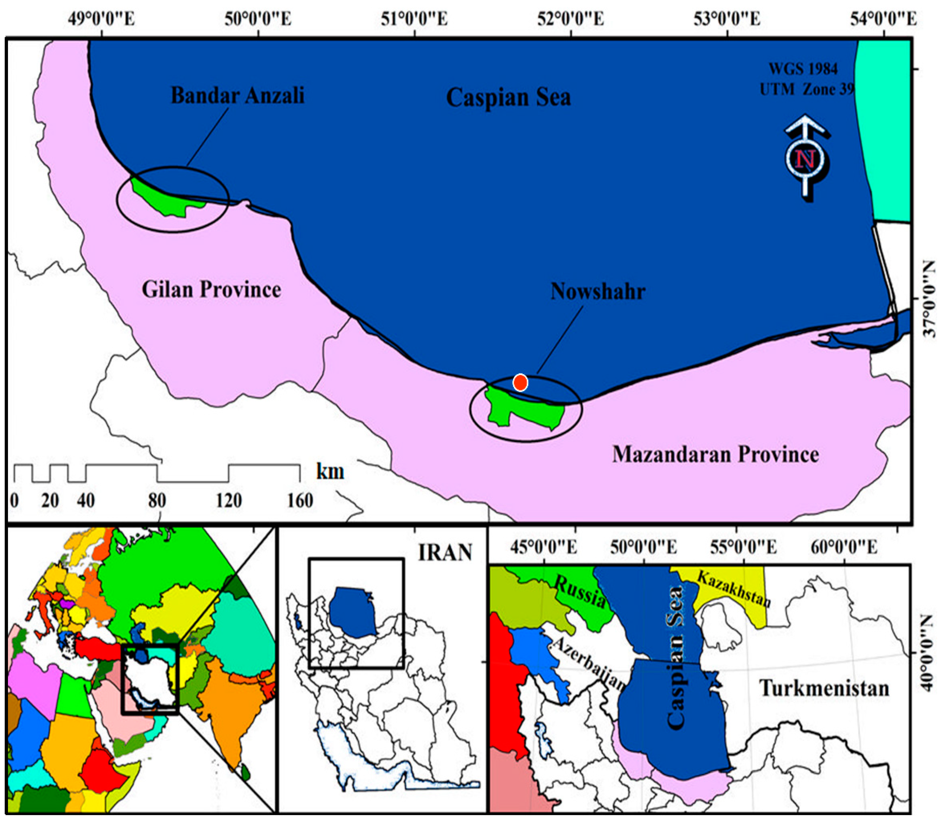
As illustrated in the following Figure 1, the study site examined in the present study is embodied by the coastal region of Mazandaran Province (northern Iran), in the southern region of the Caspian Sea. Specifically, the study area is located within the latitude of 35.47° to 36.35° and the longitude of 50.34° to 56.14°.
Having a total surface extension of about 3.9 × 10⁵ km2 and a volume of 7.8 × 10⁴ km3, the Caspian Sea region is the largest lake in the world, with an average salinity of approximately 13 ppt. It is surrounded by five countries: Azerbaijan, Iran, Kazakhstan, Russia, and Turkmenistan.
As indicated by Dyakonov and Ibrayev [58], the northern region of the Caspian Sea is shallow, with a maximum depth of about 40 m, while the middle and southern regions are strongly deeper, as testified by a peak depth of about 1025 m.
2.2. Buoy-Based Wind Waves Data
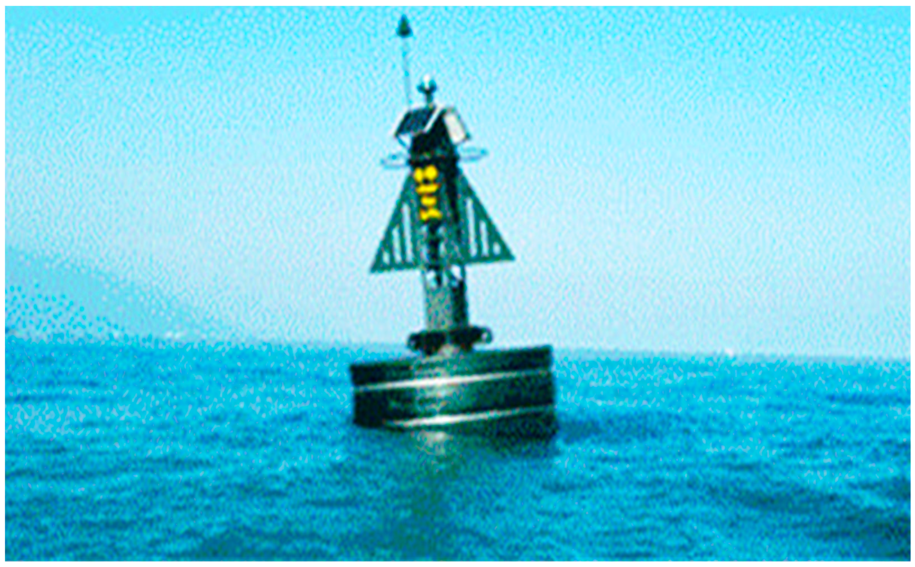
Nowshahr buoy (36°42′09″ N, 51°37′17″ E) data consist of wave heights (m), velocity, direction, and other key parameters, which were derived from the Ports and Maritime Organization Iran (PMO) in 2010, as reported in the study carried out by Lesani and Niksokhan [23]. Specifically, compared with other types, the polyethylene Nowshahr buoy made in Iran, which was employed in the present study case, requires lower regular repairs when dealing with the presence of the most common seaweeds as algae. This buoy is a set of electrical–mechanical equipment through which meteorological and oceanographic parameters can be measured. As shown in Figure 2, the buoy restraint system consists of rubber rope, chains, nylon rope, subsurface buoy, relevant fittings, and gravity anchor. The wave sensor is of the HIPPY type and can measure vertical fluctuations of water up to 10 m with an accuracy of 1.00 cm, and the roll and pitch angles are in the range of 45°. Buoy data include wave height, wind speed and direction, and other parameters such as water and air temperature, humidity, air pressure, etc.
An overview of the data indicated that they could be associated with some errors. In fact, for wave height (m) values that reached 10 m from 0.50 m, they were most probably due to signal processing issues.
2.3. Satellite Data
In the present study, case, the remote sensing-based significant wave height (m) and wind speed values were derived from datasets acquired by the well-known Jason-2 satellite (available at https://www.ncei.noaa.gov/products/jason-satellite-products, accessed on 5 June 2021). Given a spatial resolution of 0.04° under both longitude and latitude, the Jason-2 satellite was able to measure both wind speed and wave height (m) data with accuracies equal to 0.50 cm s−1 and 1.00 cm, respectively, as indicated by Dubey et al. [59] and Yu et al. [60], among other notable remote sensing-based studies and applications.
3. Results and Discussion
3.1. Wind Speed Frequency Diagrams
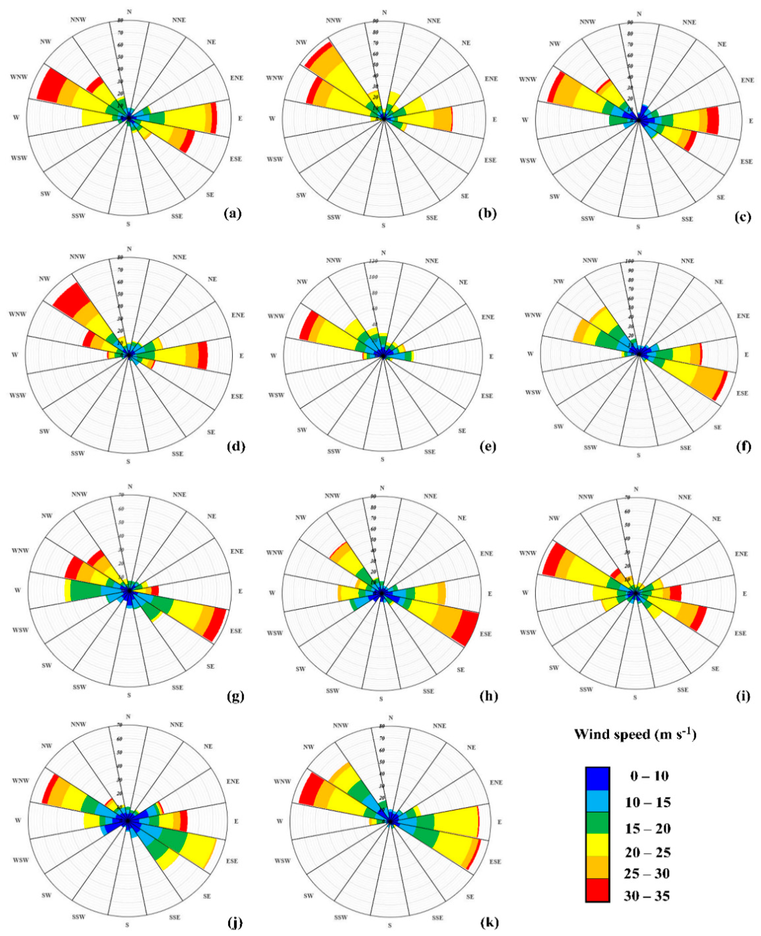
In the present study, in situ wind frequency (in percentage, %) diagrams [63] for January–November 2016 are shown in Figure 3a–k, respectively. Specifically, data were extracted from the Iranian Port and Shipping Organization and the National Oceanographic Organization of Iran, with reference to the Nowshahr buoy station.
Wind frequency (in percentage, %) diagrams were obtained by processing wind speed and direction accounting for wind speed and direction. As shown in Figure 3a, the main wind direction is WNW in January, with a shift to the NW direction in February (Figure 3b). Although the NW wind is not dominant, it is faster and has more energy. As shown in Figure 3c, the dominant wind directions in March are very similar to those observed in February, with slightly faster winds. Figure 3d displays that wind is primarily northwestern in April. In May, the wind is uniform and identical in all directions, except for the WNW directions, which show the dominant wind speed and frequencies (Figure 3e), while in June, the main wind direction is ESE, as illustrated in Figure 3f.
Figure 3g refers to July; the main wind direction is still ESE, but it exhibits higher wind speeds than in June.
In October, the wind is dominant over both WNW and ESE directions, and wind speeds are extremely similar over those directions, with a little prevalence of higher speed values over NWN. Thus, Figure 3j shows that the wind is slightly being pumped over the WNW–ESE alignment. Very similar behavior can be seen in November, as reported in Figure 3k.
3.2. Analysis of Wave Height Data
3.2.1. In Situ Data
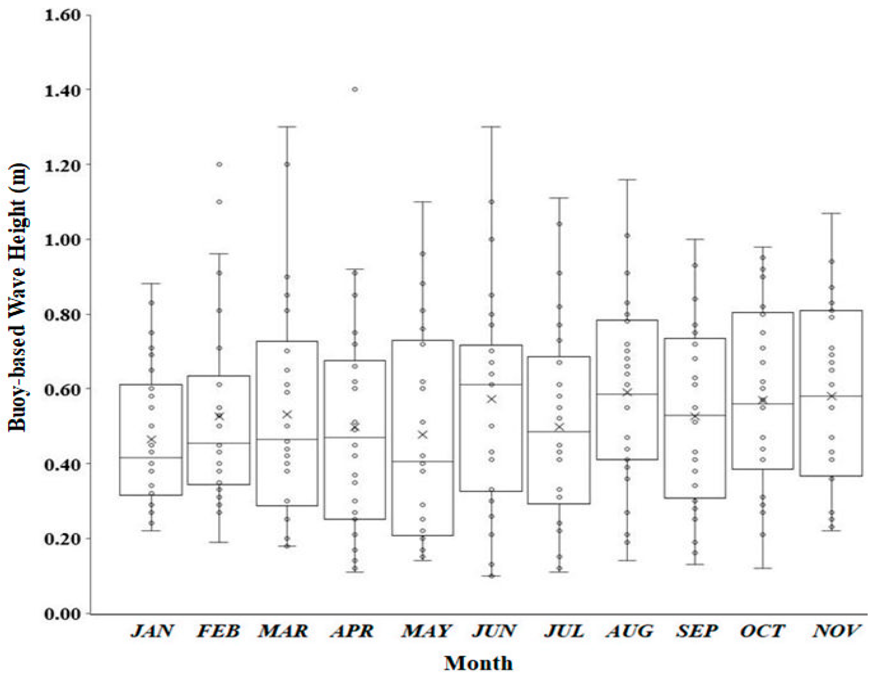
Figure 4 depicts the distributions of in situ wave height (m) data recorded at the examined buoy station in the period January–November 2016.
3.2.2. Satellite-Based Data
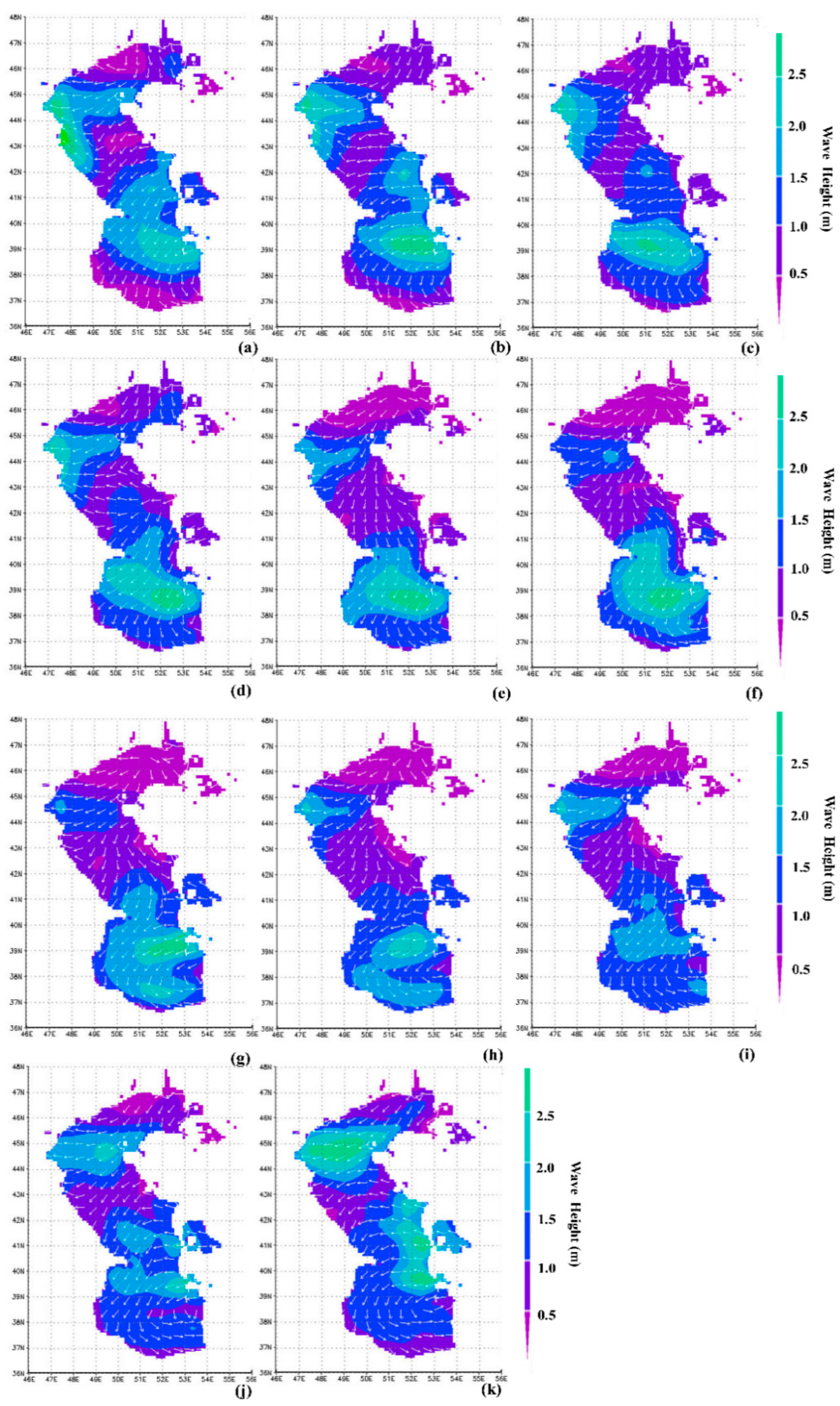
Following Kostianoy et al. [64], among others, we analyzed the monthly average wind velocity vectors and wave height (m) diagrams for the period January–November 2016, which are presented in Figure 5a–k. Each satellite altimetry-based wave height (m) map was obtained by employing the well-known Golder® Surfer v.15 software, by adopting a spatial resolution of 0.04° for both longitude and latitude.
Figure 5a shows the wind velocity pattern in January, with lower wind blowing on the southern Caspian Sea coast, and its direction from W to E, due to windage around the low-pressure region located on the E side. Given the low wind speed, a wave height of 1.00 m can be observed off the southern coast of the Caspian Sea. Figure 5b clearly shows that the weakening of the low-pressure core in the winter reduces winds blowing off-coast in February. Winds are often in W and NW. Wave height (m) on most of Mazandaran coast is about a 0.50 m and close to 1 m on the beaches of Golestan Province (36°50′19″ N, 54°26′05″ E) and Gilan Province (37°16′38″ N, 49°35′20″ E). According to the increase in seasonal winds, in March, wind developed along the S direction, with an augmentation in the length of the fetch, as shown in Figure 5c. Thus, winds decreased on the Mazandaran coast, with a very probable wave motion of higher supply wind off-coast and a wave height value of 1.00 m near the coastal area.
As shown in Figure 5d, in April, with the beginning of the warm season, wind intensity increased slightly, compared with March. The dominant wave height (m) value reached about 1.00 m or even more in this month, and the local circulation caused by the rise of higher supply temperatures witnessed an increase in wave height (m) in the middle widths, with an elevated wave higher than 1.00 m on the southern region of Caspian Sea and the coasts of Mazandaran Province. Figure 5e suggests that the dominant wind is in the N direction in May, while wind rotation in the southern part testified the existence of a low-pressure center in that region. A wave height (m) of approximately 1.00 m on the beaches is stabilized, and in such conditions, even higher waves are expected this month.
As suggested by Figure 5f, in the warmest days of June, the southern coasts of the Caspian Sea are affected by wind patterns associated with the W direction, due to the low-pressure core in the higher width. This low-pressure center continues to reduce wind size. In this case, waves are expected to be mainly associated with high-width wind speed. Despite wind speed reduction, wave height (m) on the southern coasts of the Caspian Sea flow region is less than 1.25 m.
In July, as displayed in Figure 5g, at least the elevated waves spun in a circle of low-hours over the SW region of the Caspian Sea and N portion of the Mazandaran Province. In this case, low pressure is weaker almost over Gilan Province, and its effect is expected to be directly reflected on sea wave heights (m) values at Mazandaran Province coasts. Again, with a higher NW wind intensity, far wave height (m) will reach a value equal to more than 1.00 m from the coasts. As illustrated by Figure 5h, NW wind directions are prevalent in August, with a reduction in the seasonal low-pressure center. More pressure is dispersed by the instabilities in changing low-pressure core corresponding to a slight increment in wave height (m) values at the southern region of the Caspian Sea, mainly due to augmentation in wind speed values.
In September, the low-pressure core slowly faded into the N direction in a round-clock drive off the coast of the Golestan Province, and the dominant wind is opened off the Mazandaran coast, as shown in Figure 5i. Significant wave heights of about 1.00 m can be still observed. As it can be observed from the analysis of Figure 5j, the dominant wind direction is still the western one in October, associated with the pervasive presence of a 10 knots high-intensity wind center over the beaches of the Mazandaran Province. Specifically, an NW wind pattern is clearly recognizable, and a low-pressure wind center can be identified across the NW region of the Caspian Sea area. Finally, as reported in Figure 5k, multiple western winds can be identified in November, having a speed of about 10 knots on the coastal area.
Lower stability of wind direction and narrower fetches induced a slower sea flow across the Caspian Sea region in October and November, while the dominant wave height (m) on the coasts of the Mazandaran Province is about 0.00—1.00 m, mainly due to an increase in the low-pressure core, reducing both wind speed and rotation and shortening the fetch’s length.
3.3. Comparative Analysis
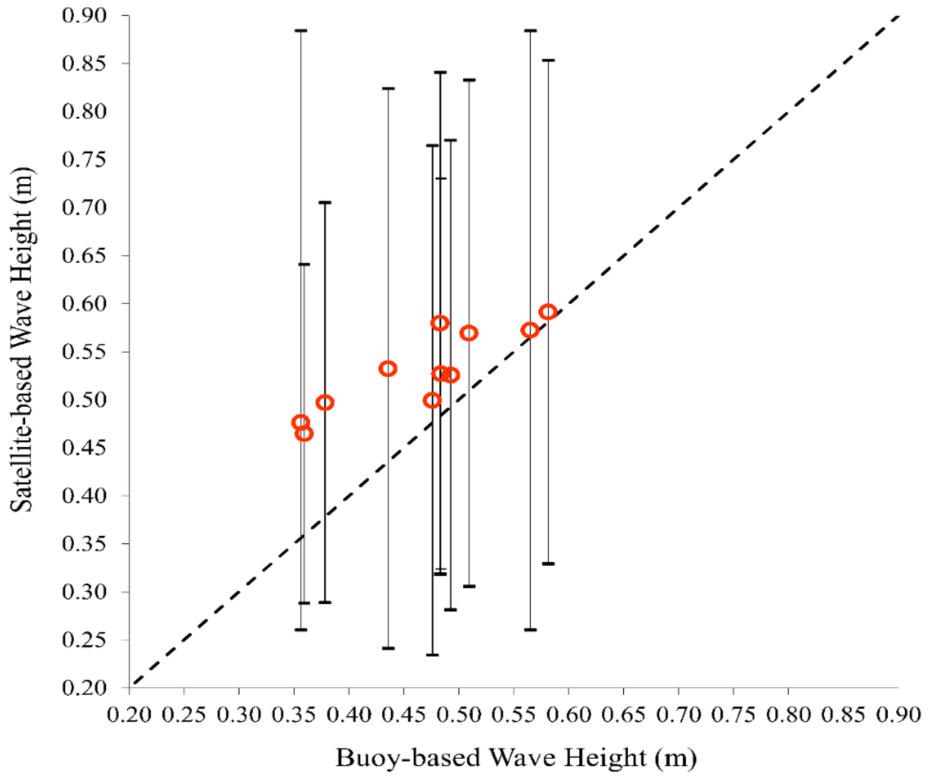
Figure 6 shows the comparative analysis carried out for the period January–November 2016 between monthly average buoy-based and monthly average satellite-based wave height (m) data over the southern coasts of the Caspian Sea.
Finally, as illustrated in Figure 6, in this study, a good correlation was observed between average buoy-based and average satellite-based wave heights (m) over the southern coasts of the Caspian Sea, associated with a slight overestimation in all the examined months. These values exhibit a high correlation, as can be easily detected from a value of correlation coefficient r equal to 0.87, with values of bias and RMSE equal to 0.063 m and 0.071 m, respectively. The statistical performances obtained after the comparative analysis carried out here highly agree with the outcomes of the comparative study carried out by Lo Feudo et al. [40], in which the RMSE was equal to 0.091 m.
It is important to highlight that for, both SAR and altimetry, wave heights errors can occur, especially for low wave heights.
A substantial improvement in the predictive performance of the indirect sea wave estimations obtained in the present study case can be reached by combining them with the most advanced methods for the quantitative assessment of stochastic uncertainty propagation [65,66,67,68,69,70,71,72], as reported by previous environmental and ecohydraulic engineering studies [73,74,75,76,77,78,79,80].
4. Conclusions
It was possible to assess from the analysis of the outcomes of satellite-based processing that the minimum wave height (m) values were obtained in May and June. An active low-pressure system was registered in the Caspian Sea area, located in the NW direction in January, which provided a clockwise rotation for the whole year. This flow system is the main reason for the changes in wind speed and direction, also playing a key role in wave height (m) assessments for the coasts of Mazandaran Province. Except for the time limit conditions occurring when the low-pressure mass is dominant on the SE coast, satellite-based wave height (m) values rarely exceed 1.00 m across the coasts of the Caspian Sea.
The outcomes of the present study represent, for the first time, an interesting research goal in terms of accurate wave height (m) data within the southern coasts of the Caspian Sea, characterized by highly unpredictable fluid dynamics, environmental, and wind patterns.
Additionally, it is possible to conclude that satellite-based data is highly accurate and more suitable given its comprehensive nature, compared with buoy-based ones, in terms of both spatial resolution and measuring technique.
Author Contributions
Conceptualization, G.F.C.L., T.S., M.T.A., P.S. and O.K.; methodology, G.F.C.L., T.S., M.T.A., P.S. and O.K.; validation, G.F.C.L., T.S., M.T.A., P.S. and O.K.; investigation, G.F.C.L., T.S., M.T.A., P.S. and O.K.; data curation, G.F.C.L., T.S., M.T.A., P.S. and O.K.; writing—original draft preparation, G.F.C.L., T.S., M.T.A. and P.S.; writing—review and editing, G.F.C.L., T.S., M.T.A., P.S. and O.K. All authors have read and agreed to the published version of the manuscript.
Funding
This research received no external funding.
Informed Consent Statement
Informed consent was obtained from all subjects involved in the study.
Data Availability Statement
The data presented in this study are available on request from the corresponding author.
Acknowledgments
The authors want to thank Eng. Rämäbär Pänø for his considerable support during the pre- and postprocessing analyses, in the case of both satellite- and buoy-based sea wave data examined in the comparative analyses performed in this study.
Conflicts of Interest
The authors declare no conflict of interest.
References
- Jia, N.; Zhao, D. The Influence of Wind Speed and Sea States on Whitecap Coverage. J. Ocean Univ. China 2019, 18, 282–292. [Google Scholar] [CrossRef]
- Crimaldi, M.; Lama, G.F.C. Impact of riparian plants biomass assessed by UAV-acquired multispectral images on the hydrodynamics of vegetated streams. In Proceedings of the 29th European Biomass Conference and Exhibition, Online, 26–29 April 2021; pp. 1157–1161. [Google Scholar]
- Capolupo, A.; Monterisi, C.; Saponieri, A.; Addona, F.; Damiani, L.; Archetti, R.; Tarantino, E. An Interactive WebGIS Framework for Coastal Erosion Risk Management. J. Mar. Sci. Eng. 2021, 9, 567. [Google Scholar] [CrossRef]
- Lama, G.F.C.; Crimaldi, M. Assessing the role of Gap Fraction on the Leaf Area Index (LAI) estimations of riparian vegetation based on Fisheye lenses. In Proceedings of the 29th European Biomass Conference and Exhibition, Online, 26–29 April 2021; pp. 1172–1176. [Google Scholar]
- Marcos, M.; Wöppelmann, G.; Matthews, A.; Ponte, R.M.; Birol, F.; Ardhuin, F.; Chambers, D. Coastal Sea level and related fields from existing observing systems. Surv. Geophys. 2019, 40, 1293–1317. [Google Scholar] [CrossRef] [Green Version]
- Divinsky, B.V.; Fomin, V.V.; Kosyan, R.D.; Ratner, Y.D. Extreme wind waves in the Black Sea. Oceanologia 2021, 62, 23–30. [Google Scholar] [CrossRef]
- Hwang, P.A.; Reul, N.; Meissner, T.; Yueh, S.H. Whitecap and Wind Stress Observations by Microwave Radiometers: Global Coverage and Extreme Conditions. J. Phys. Oceanogr. 2019, 49, 2291–2307. [Google Scholar] [CrossRef]
- Meucci, A.; Young, I.R.; Aarnes, O.J.; Breivik, Ø. Comparison of Wind Speed and Wave Height Trends from Twentieth-Century Models and Satellite Altimeters. J. Clim. 2020, 33, 611–624. [Google Scholar] [CrossRef]
- Lama, G.F.C.; Chirico, G.B. Effects of reed beds management on the hydrodynamic behaviour of vegetated open channels. In Proceedings of the 2020 IEEE International Workshop on Metrology for Agriculture and Forestry (MetroAgriFor), Trento, Italy, 4–6 November 2020; pp. 149–154. [Google Scholar] [CrossRef]
- Dodet, G.; Mélet, A.; Ardhuin, F.; Bertin, X.; Idier, D.; Almar, R. The contribution of wind-generated waves to coastal sea-level changes. Surv. Geophys. 2019, 40, 1563–1601. [Google Scholar] [CrossRef] [Green Version]
- Lama, G.F.C.; Errico, A.; Francalanci, S.; Solari, L.; Preti, F.; Chirico, G.B. Evaluation of Flow Resistance Models Based on Field Experiments in a Partly Vegetated Reclamation Channel. Geosciences 2020, 10, 47. [Google Scholar] [CrossRef] [Green Version]
- Bishop, C.T.; Donelan, M.A.; Kahma, K.K. Shore protection manual’s wave prediction reviewed. Coast. Eng. 1992, 17, 25–48. [Google Scholar] [CrossRef]
- Shore Protection Manual; U.S. Govt. Printing Office: Washington, DC, USA, 1984; Volume 1–2.
- Altunkaynak, A. Prediction of significant wave height using geno-multilayer perceptron. Ocean Eng. 2013, 58, 144–153. [Google Scholar] [CrossRef]
- Duffy, M.; Devoy, R. Contemporary process controls on the evolution of sedimentary coasts under low to high energy regimes: Western Ireland. Geol. Mijnb. 1998, 77, 333–349. [Google Scholar] [CrossRef] [Green Version]
- Etemad-Shahidi, A.; Mahjoobi, J. Comparison between M5′ model tree and neural networks for prediction of significant wave height in Lake Superior. Ocean Eng. 2009, 36, 1175–1181. [Google Scholar] [CrossRef]
- Durán-Rosal, A.M.; Hervás-Martínez, C.; Tallón-Ballesteros, A.J.; Martínez-Estudillo, A.C.; Salcedo-Sanz, S. Massive missing data reconstruction in ocean buoys with evolutionary product unit neural networks. Ocean Eng. 2016, 117, 292–301. [Google Scholar] [CrossRef]
- Eleveld, M.A. Wind-induced resuspension in a shallow lake from Medium Resolution Imaging Spectrometer (MERIS) full-resolution reflectances. Water Resour. Res. 2012, 48, W04508. [Google Scholar] [CrossRef] [Green Version]
- Kang, S.-L.; Won, H. Spectral structure of 5 year time series of horizontal wind speed at the Boulder Atmospheric Observatory. J. Geophys. Res. Atmos. 2016, 121, 11946–11967. [Google Scholar] [CrossRef]
- West, C.G.; Smith, R.B. Global patterns of offshore wind variability. Wind Energy 2021, 24, 1466–1481. [Google Scholar] [CrossRef]
- Sarno, L.; Wang, Y.; Tai, Y.-C.; Martino, R.; Carravetta, A. Asymptotic analysis of the eigenstructure of the two-layer model and a new family of criteria for evaluating the model hyperbolicity. Adv. Water Resour. 2021, 154, 103966. [Google Scholar] [CrossRef]
- Fontana, M.; Casalone, P.; Sirigu, S.A.; Giorgi, G.; Bracco, G.; Mattiazzo, G. Viscous Damping Identification for a Wave Energy Converter Using CFD-URANS Simulations. J. Mar. Sci. Eng. 2020, 8, 355. [Google Scholar] [CrossRef]
- Lesani, S.; Niksokhan, M.H. Climate change impact on Caspian Sea wave conditions in the Noshahr Port. Ocean Dyn. 2019, 69, 1287–1310. [Google Scholar] [CrossRef]
- Davidson, J.; Costello, R. Efficient Nonlinear Hydrodynamic Models for Wave Energy Converter Design—A Scoping Study. J. Mar. Sci. Eng. 2020, 8, 35. [Google Scholar] [CrossRef] [Green Version]
- Ogawa, H.; Dickson, M.E.; Kench, P.S. Hydrodynamic constraints and storm wave characteristics on a sub-horizontal shore platform. Earth Surf. Process. Landf. 2014, 40, 65–77. [Google Scholar] [CrossRef]
- Berta, M.; Bellomo, L.; Griffa, A.; Magaldi, M.G.; Molcard, A.; Mantovani, C.; Gasparini, G.P.; Marmain, J.; Vetrano, A.; Béguery, L.; et al. Wind-induced variability in the Northern Current (northwestern Mediterranean Sea) as depicted by a multi-platform observing system. Ocean Sci. 2018, 14, 689–710. [Google Scholar] [CrossRef] [Green Version]
- Melet, A.; Meyssignac, B.; Almar, R.; Le Cozannet, G. Under-estimated wave contribution to coastal sea-level rise. Nat. Clim. Chang. 2018, 8, 234–239. [Google Scholar] [CrossRef]
- Cecilio, R.O.; Dillenburg, S.R. An ocean wind-wave climatology for the Southern Brazilian Shelf. Part II: Variability in space and time. Dyn. Atmos. Ocean. 2019, 88, 101103. [Google Scholar] [CrossRef]
- Lama, G.F.C.; Rillo Migliorini Giovannini, M.; Errico, A.; Mirzaei, S.; Padulano, R.; Chirico, G.B.; Preti, F. Hydraulic Efficiency of Green-Blue Flood Control Scenarios for Vegetated Rivers: 1D and 2D Unsteady Simulations. Water 2021, 13, 1333. [Google Scholar] [CrossRef]
- Grigorieva, V.G.; Gulev, S.K.; Sharmar, V.D. Validating Ocean Wind Wave Global Hindcast with Visual Observations from VOS. Oceanology 2020, 60, 9–19. [Google Scholar] [CrossRef]
- Penna, N.T.; Morales Maqueda, M.A.; Martin, I.; Guo, J.; Foden, P.R. Sea surface height measurement using a GNSS Wave Glider. Geophys. Res. Lett. 2018, 45, 5609–5616. [Google Scholar] [CrossRef]
- Badulin, S.I. A physical model of sea wave period from altimeter data. J. Geophys. Res. Oceans 2014, 119, 856–869. [Google Scholar] [CrossRef] [Green Version]
- Rosmorduc, V.; Srinivasan, M.; Richardson, A.; Cipollini, P. The first 25 years of altimetry outreach. Adv. Space Res. 2020, 68, 1225–1241. [Google Scholar] [CrossRef]
- Lebedev, S.A. Mean Sea Surface Model of the Caspian Sea Based on TOPEX/Poseidon and Jason-1 Satellite Altimetry Data. In Geodesy for Planet Earth. International Association of Geodesy Symposia; Kenyon, S., Pacino, M., Marti, U., Eds.; Springer: Berlin/Heidelberg, Germany, 2012; Volume 136. [Google Scholar] [CrossRef]
- Zecchetto, S. Wind Direction Extraction from SAR in Coastal Areas. Remote Sens. 2018, 10, 261. [Google Scholar] [CrossRef] [Green Version]
- Sorkhabi, O.M.; Asgari, J.; Amiri-Simkooei, A. Monitoring of Caspian Sea-level changes using deep learning-based 3D reconstruction of GRACE signal. Measurement 2021, 174, 109004. [Google Scholar] [CrossRef]
- Khatibi, R.; Ghorbani, M.A.; Naghshara, S.; Aydin, H.; Karimi, V. A framework for ‘Inclusive Multiple Modelling’ with critical views on modelling practices—Applications to modelling water levels of Caspian Sea and Lakes Urmia and Van. J. Hydrol. 2020, 587, 124923. [Google Scholar] [CrossRef]
- Arnell, N.W.; Gosling, S.N. The impacts of climate change on river flood risk at the global scale. Clim. Chang. 2016, 134, 387–401. [Google Scholar] [CrossRef] [Green Version]
- Tao, J.; Guosheng, L. Contemporary monitoring of storm surge activity. Prog. Phys. Geogr. 2019, 44, 299–314. [Google Scholar] [CrossRef]
- Giorgi, F.; Bi, X.; Pal, J. Mean, interannual variability and trends in a regional climate change experiment over Europe. II: Climate change scenarios (2071–2100). Clim. Dyn. 2004, 23, 839–858. [Google Scholar] [CrossRef]
- Lo Feudo, T.; Mel, R.A.; Sinopoli, S.; Maiolo, M. Wave Climate and Trends for the Marine Experimental Station of Capo Tirone Based on a 70-Year-Long Hindcast Dataset. Water 2022, 14, 163. [Google Scholar] [CrossRef]
- Lebedev, S.A.; Kostianoy, A.G. Integrated use of satellite altimetry in the investigation of the meteorological- hydrological, and hydrodynamic regime of the Caspian Sea. Terr. Atmos. Ocean. Sci. 2008, 19, 71–82. [Google Scholar] [CrossRef] [Green Version]
- Lama, G.F.C.; Crimaldi, M.; Pasquino, V.; Padulano, R.; Chirico, G.B. Bulk Drag Predictions of Riparian Arundo donax Stands through UAV-Acquired Multispectral Images. Water 2021, 13, 1333. [Google Scholar] [CrossRef]
- De Padova, D.; Calvo, L.; Carbone, P.M.; Maraglino, D.; Mossa, M. Comparison between the Lagrangian and Eulerian Approach for Simulating Regular and Solitary Waves Propagation, Breaking and Run-Up. Appl. Sci. 2021, 11, 9421. [Google Scholar] [CrossRef]
- Mossa, M.; Meftah, M.B.; De Serio, F.; Nepf, H.M. How vegetation in flows modifies the turbulent mixing and spreading of jets. Sci. Rep. 2017, 7, 6587. [Google Scholar] [CrossRef] [Green Version]
- Ribal, A.; Young, I.R. 33 years of globally calibrated wave height and wind speed data based on altimeter observations. Sci. Data 2019, 6, 77. [Google Scholar] [CrossRef] [PubMed] [Green Version]
- Derkani, M.H.; Alberello, A.; Nelli, F.; Bennetts, L.G.; Hessner, K.G.; MacHutchon, K.; Reichert, K.; Aouf, L.; Khan, S.; Toffoli, A. Wind, waves, and surface currents in the Southern Ocean: Observations from the Antarctic Circumnavigation Expedition. Earth Syst. Sci. Data 2021, 13, 1189–1209. [Google Scholar] [CrossRef]
- Heron, S.F.; Heron, M.L. A Comparison of Algorithms for Extracting Significant Wave Height from HF Radar Ocean Backscatter Spectra. J. Atmos. Ocean Technol. 1998, 15, 1157–1163. [Google Scholar] [CrossRef]
- Roarty, H.; Cook, T.; Hazard, L.; George, D.; Harlan, J.; Cosoli, S.; Wyatt, L.; Alvarez Fanjul, E.; Terrill, E.; Otero, M.; et al. The Global High Frequency Radar Network. Front. Mar. Sci. 2019, 6, 164. [Google Scholar] [CrossRef]
- Zhou, H.; Wen, B. Wave height estimation using the singular peaks in the sea echoes of high frequency radar. Acta Oceanol. Sin. 2018, 37, 108–114. [Google Scholar] [CrossRef]
- Lai, Y.; Wang, Y.; Zhou, H. First-Order Peaks Determination for Direction-Finding High-Frequency Radar. J. Mar. Sci. Eng. 2021, 9, 8. [Google Scholar] [CrossRef]
- Wyatt, L.R.; Green, J.J.; Middleditch, A. HF radar data quality requirements for wave measurement. Coast. Eng. 2011, 58, 327–336. [Google Scholar] [CrossRef]
- You, J.; Faltinsen, O.M. A numerical investigation of second-order difference-frequency forces and motions of a moored ship in shallow water. J. Ocean Eng. Mar. Energy 2015, 1, 157–179. [Google Scholar] [CrossRef] [Green Version]
- Barrick, D.; Fernandez, V.; Ferrer, M.I.; Whelan, C.; Breivik, Ø. A short-term predictive system for surface currents from a rapidly deployed coastal HF radar network. Ocean Dyn. 2012, 62, 725–740. [Google Scholar] [CrossRef]
- Coe, R.G.; Bacelli, G.; Forbush, D. A practical approach to wave energy modeling and control. Renew. Sustain. Energy Rev. 2021, 142, 110791. [Google Scholar] [CrossRef]
- Rijnsdorp, D.P.; Zijlema, M. Simulating waves and their interactions with a restrained ship using a non-hydrostatic wave-flow model. Coast. Eng. 2016, 114, 119–136. [Google Scholar] [CrossRef] [Green Version]
- Wang, X.; Ichikawa, K. Effect of High-Frequency Sea Waves on Wave Period Retrieval from Radar Altimeter and Buoy Data. Remote Sens. 2016, 8, 764. [Google Scholar] [CrossRef] [Green Version]
- Dyakonov, G.S.; Ibrayev, R.A. Long-term evolution of Caspian Sea thermohaline properties reconstructed in an eddy-resolving ocean general circulation model. Ocean Sci. 2019, 15, 527–541. [Google Scholar] [CrossRef] [Green Version]
- Dubey, A.K.; Gupta, P.K.; Dutta, S.; Singh, R.P. An improved methodology to estimate river stage and discharge using Jason-2 satellite data. J. Hydrol. 2015, 529, 1776–1787. [Google Scholar] [CrossRef]
- Yu, H.; Li, J.; Wu, K.; Wang, Z.; Yu, H.; Zhang, S.; Hou, Y.; Kelly, R.M. A global high-resolution ocean wave model improved by assimilating the satellite altimeter significant wave height. Int. J. Appl. Earth Obs. Geoinf. 2018, 70, 43–50. [Google Scholar] [CrossRef]
- Xie, J.; Wang, X.; Yang, Z.; Hao, S. Virtual monitoring method for hydraulic supports based on digital twin theory. Min. Technol. 2019, 128, 77–87. [Google Scholar] [CrossRef]
- Yan, J.; Ma, Y.; Wang, L.; Choo, K.-K.R.; Jie, W. A cloud-based remote sensing data production system. Future Gener. Comput. Syst. 2018, 86, 1154–1166. [Google Scholar] [CrossRef] [Green Version]
- Carlson, D.F.; Griffa, A.; Zambianchi, E.; Suaria, G.; Corgnati, L.; Magaldi, M.G.; Poulain, P.-M.; Russo, A.; Bellomo, L.; Mantovani, C.; et al. Observed and modeled surface Lagrangian transport between coastal regions in the Adriatic Sea with implications for marine protected areas. Cont. Shelf Res. 2016, 118, 23–48. [Google Scholar] [CrossRef]
- Kostianoy, A.G.; Ginzburg, A.I.; Lavrova, O.Y.; Lebedev, S.A.; Mityagina, M.I.; Sheremet, N.A.; Soloviev, D.M. Comprehensive Satellite Monitoring of Caspian Sea Conditions. In Remote Sensing of the Asian Seas; Barale, V., Gade, M., Eds.; Springer: Cham, Switzerland, 2019. [Google Scholar] [CrossRef]
- Padulano, R.; Lama, G.F.C.; Rianna, G.; Santini, M.; Mancini, M.; Stojiljkovic, M. Future rainfall scenarios for the assessment of water availability in Italy. In Proceedings of the 2020 IEEE International Workshop on Metrology for Agriculture and Forestry (MetroAgriFor), Trento, Italy, 4–6 November 2020; pp. 241–246. [Google Scholar] [CrossRef]
- Severino, G.; Leveque, S.; Toraldo, G. Uncertainty quantification of unsteady source flows in heterogeneous porous media. J. Fluid Mech. 2019, 870, 5–26. [Google Scholar] [CrossRef]
- Lama, G.F.C.; Errico, A.A.; Francalanci, S.; Solari, L.; Preti, F.; Chirico, G.B. Comparative analysis of modelled and measured vegetative Chézy’s flow resistance coefficients in a drainage channel vegetated by dormant riparian reed. In Proceedings of the International IEEE Workshop on Metrology for Agriculture and Forestry, Portici, Italy, 24–26 October 2019; pp. 180–184. [Google Scholar] [CrossRef]
- Szeląg, B.; Suligowski, R.; Drewnowski, J.; De Paola, F.; Fernandez-Morales, F.J.; Bąk, Ł. Simulation of the number of storm overflows considering changes in precipitation dynamics and the urbanisation of the catchment area: A probabilistic approach. J. Hydrol. 2021, 598, 126275. [Google Scholar] [CrossRef]
- Lama, G.F.C.; Rillo Migliorini Giovannini, M.; Errico, A.; Mirzaei, S.; Chirico, G.B.; Preti, F. The impacts of Nature Based Solutions (NBS) on vegetated flows’ dynamics in urban areas. In Proceedings of the 2021 IEEE International Workshop on Metrology for Agriculture and Forestry (MetroAgriFor), Trento-Bolzano, Italy, 3–5 November 2021; pp. 58–63. [Google Scholar] [CrossRef]
- Severino, G.; Cuomo, S.; Sommella, A.; D’Urso, G. On the longitudinal dispersion in conservative transport through heterogeneous porous formations at finite Peclet numbers. Water Resour. Res. 2017, 53, 8614–8625. [Google Scholar] [CrossRef]
- Lama, G.F.C.; Crimaldi, M.; De Vivo, A.; Chirico, G.B.; Sarghini, F. Eco-hydrodynamic characterization of vegetated flows derived by UAV-based imagery. In Proceedings of the 2021 IEEE International Workshop on Metrology for Agriculture and Forestry (MetroAgriFor), Trento-Bolzano, Italy, 3–5 November 2021; pp. 273–278. [Google Scholar] [CrossRef]
- Di Cristo, C.; Iervolino, M.; Vacca, A.; Zanuttigh, B. Roll-waves prediction in dense granular flows. J. Hydrol. 2009, 77, 50–58. [Google Scholar] [CrossRef]
- Lama, G.F.C.; Errico, A.; Francalanci, S.; Solari, L.; Chirico, G.B.; Preti, F. Hydraulic Modeling of Field Experiments in a Drainage Channel Under Different Riparian Vegetation Scenarios. In Innovative Biosystems Engineering for Sustainable Agriculture, Forestry and Food Production; Lecture Notes in Civil Engineering; Coppola, A., Di Renzo, G., Altieri, G., D’Antonio, P., Eds.; Springer International Publishing: Cham, Switzerland, 2020; pp. 69–77. [Google Scholar] [CrossRef]
- Fallico, C.; De Bartolo, S.; Brunetti, G.F.A.; Severino, G. Use of fractal models to define the scaling behavior of the aquifers’ parameters at the mesoscale. Stoch. Environ. Res. Risk Assess. 2021, 35, 971–984. [Google Scholar] [CrossRef]
- Sadeghifar, T.; Lama, G.F.C.; Sihag, P.; Bayram, A.; Kisi, O. Wave height predictions in complex sea flows through soft computing models: Case study of Persian Gulf. Ocean Eng. 2022, 245, 110467. [Google Scholar] [CrossRef]
- Avino, A.; Manfreda, S.; Cimorelli, L.; Pianese, D. Trend of annual maximum rainfall in Campania region (Southern Italy). Hydrol. Process. 2021, 35, e14447. [Google Scholar] [CrossRef]
- Sadeghifar, T.; Nouri Motlagh, M.; Torabi Azad, M.; Mohammad Mahdizadeh, M. Coastal wave height prediction using Recurrent Neural Networks (RNNs) in the south Caspian Sea. Mar. Geod. 2017, 40, 454–465. [Google Scholar] [CrossRef]
- Buccino, M.; Tuozzo, S.; Ciccaglione, M.C.; Calabrese, M. Predicting Crenulate Bay Profiles from Wave Fronts: Numerical Experiments and Empirical Formulae. Geosciences 2021, 11, 208. [Google Scholar] [CrossRef]
- Errico, A.; Lama, G.F.C.; Francalanci, S.; Chirico, G.B.; Solari, L.; Preti, F. Flow dynamics and turbulence patterns in a drainage channel colonized by common reed (Phragmites australis) under different scenarios of vegetation management. Ecol. Eng. 2019, 133, 39–52. [Google Scholar] [CrossRef]
- Saponaro, M.; Agapiou, A.; Hadjimitsis, D.G.; Tarantino, E. Influence of Spatial Resolution for Vegetation Indices’ Extraction Using Visible Bands from Unmanned Aerial Vehicles’ Orthomosaics Datasets. Remote Sens. 2021, 13, 3238. [Google Scholar] [CrossRef]
Figure 1.
Detailed map of southern coasts of the Caspian Sea area, with a wide overview of the locations of Nowshahr buoy station (northern Iran). Additionally, an overview of all countries surrounding southern Caspian Sea area (Azerbaijan, Iran, Kazakhstan, Russia, and Turkmenistan) is reported in Figure 1. The orange marker indicates the location of Nowshahr buoy.

Figure 2.
View of Nowshahr buoy (36°42′09″ N, 51°37′17″ E). Courtesy of Ports and Maritime Organization Iran (PMO).
Figure 2.
View of Nowshahr buoy (36°42′09″ N, 51°37′17″ E). Courtesy of Ports and Maritime Organization Iran (PMO).

Figure 3.
Wind frequency (in percentage, %) diagrams at (a) January, (b) February, (c) March, (d) April, (e) May, (f) June, (g) July, (h) August, (i) September, (j) October, and (k) November 2016.
Figure 3.
Wind frequency (in percentage, %) diagrams at (a) January, (b) February, (c) March, (d) April, (e) May, (f) June, (g) July, (h) August, (i) September, (j) October, and (k) November 2016.

Figure 4.
Box plots of buoy-based wave height (m) data over the southern coasts of Caspian Sea region from January to November 2016. The cross indicates the mean of the distribution, while the circles indicate the single buoy-based wave height (m) value.
Figure 4.
Box plots of buoy-based wave height (m) data over the southern coasts of Caspian Sea region from January to November 2016. The cross indicates the mean of the distribution, while the circles indicate the single buoy-based wave height (m) value.

Figure 5.
Detailed maps of monthly mean satellite-based wave heights (m) over Caspian Sea flow area in (a) January, (b) February, (c) March, (d) April, (e) May, (f) June, (g) July, (h) August, (i) September, (j) October, and (k) November 2016. The white arrows in all figures indicate the wind velocities, with arrows’ length proportional to speed magnitude, based on 10 knots unit.

Figure 6.
Comparative analysis of monthly average buoy- and satellite-based wave heights (m) over the southern coasts of Caspian Sea flow area in January–November. The black dashed line represents the perfect agreement, while the vertical bars indicate the error bars in terms of ± standard deviation.

Publisher’s Note: MDPI stays neutral with regard to jurisdictional claims in published maps and institutional affiliations. |
© 2022 by the authors. Licensee MDPI, Basel, Switzerland. This article is an open access article distributed under the terms and conditions of the Creative Commons Attribution (CC BY) license (https://creativecommons.org/licenses/by/4.0/).
Share and Cite
MDPI and ACS Style
Lama, G.F.C.; Sadeghifar, T.; Azad, M.T.; Sihag, P.; Kisi, O. On the Indirect Estimation of Wind Wave Heights over the Southern Coasts of Caspian Sea: A Comparative Analysis. Water 2022, 14, 843. https://doi.org/10.3390/w14060843
AMA Style
Lama GFC, Sadeghifar T, Azad MT, Sihag P, Kisi O. On the Indirect Estimation of Wind Wave Heights over the Southern Coasts of Caspian Sea: A Comparative Analysis. Water. 2022; 14(6):843. https://doi.org/10.3390/w14060843
Chicago/Turabian StyleLama, Giuseppe Francesco Cesare, Tayeb Sadeghifar, Masoud Torabi Azad, Parveen Sihag, and Ozgur Kisi. 2022. "On the Indirect Estimation of Wind Wave Heights over the Southern Coasts of Caspian Sea: A Comparative Analysis" Water 14, no. 6: 843. https://doi.org/10.3390/w14060843
Note that from the first issue of 2016, this journal uses article numbers instead of page numbers. See further details here.