Seasonal Dynamics of Algal Net Primary Production in Response to Phosphorus Input in a Mesotrophic Subtropical Plateau Lake, Southwestern China

Abstract

A comprehensive 3-dimensional hydrodynamic and eutrophication model, the environmental fluid dynamics code model (EFDC) with three functional phytoplankton groups, was applied to simulate the algal dynamics in a mesotrophic P-limited subtropical plateau lake, Lake Erhai, Southwestern China. Field investigations revealed the seasonal patterns in external total phosphorus (TP) input and TP concentration, as well as the composition of the phytoplankton community. The model was calibrated to reproduce qualitative features and the succession of phytoplankton communities, and the net primary production was calculated. The modeled daily net primary production (NPP) ranged between −16.89 and 15.12 mg C/m²/d and exhibited significant seasonal variation. The competition for phosphorus and temperature was identified as the primary governing factor of NPP by analyzing the parameter sensitivity and limitation factors of the lake. The simulation of four nutrient loading reduction scenarios suggested high phytoplankton biomass and NPP sensitivity to the external TP reduction. A significant positive correlation was found among NPP, total phytoplankton biomass and TP concentration. Overall, this work offers an alternative approach to estimating lake NPP, which has the potential to improve sustainable lake management.

1. Introduction

In recent decades, the global spread of water eutrophication has become a critical issue of importance and research interest [1,2,3]. Nutrients, referring to nitrogen (N) and phosphorus (P) and biogeochemical cycles in lake watersheds are strongly influenced by the input of anthropogenic nutrients via river runoffs [4,5,6]. The oversupply of nutrients always leads to eutrophication, which results in elevated gross primary productivity (GPP), net primary production (NPP) and a high level of chlorophyll (Chla) [7,8,9]. NPP, defined as the net accumulation rate of carbon, is among the critical properties of ecosystems, which not only forms the basis of food webs, but also influences ecosystem-scale biogeochemical cycling rates. Surveys of NPP across stressor gradients can also help to identify how environmental change and anthropogenic disturbance alter metabolism rates in aquatic ecosystems [10,11,12]. Accordingly, understanding and forecasting the changes in NPP in response to external forcings, such as phosphorus, are major challenges for both scientific issues and improving sustainable lake management.

To date, several approaches have been developed to estimate NPP, including bottle and chamber incubations [13,14], the diel open-water technique [15,16,17] and oxygen isotopes [18,19]. However, the high temporal and spatial heterogeneity of NPP has posed a challenge in generating a comprehensive assessment of NPP in large and deep lakes. In addition to direct measurement, indirect estimation using alternative metrics (e.g., Chla and algal biomass) has also been utilized, including mathematical modeling approaches [20,21,22]. NPP is generally regulated by several biochemical and physical processes, such as temperature, light, nutrient availability, and water current [23,24,25,26,27,28]. Consequently, most recent works modeling the NPP are concerned with related parameters [29,30,31]. In addition, NPP is also influenced by biochemical differences in the algal community; the dominant species composition varies seasonally, but fewer studies dealing with NPP change in response to the shifting of the dominant species composition.

The Environmental Fluid Dynamics Code (EFDC) [32] is a comprehensive multi-dimensional surface water model that has been widely utilized for a wide range of water body types. The eutrophication module of EFDC is a carbon-based sub-model, simulating carbon dynamics in the lake. Moreover, the simulation of phytoplankton in EFDC is divided into three algal groups (diatoms, green algae and cyanobacteria). The division makes it possible to achieve the seasonal algal group transitions to investigate the species-specific impact on NPP. Therefore, we believe that the EFDC model could be utilized to model the NPP of the lake and reflect the effects of dominant species changes in phytoplankton on NPP. Although few comparative studies are available, the results are promising. Qin and Shen [33] determined the impact of local and transport processes on phytoplankton primary production using the EFDC model. Camacho et al. [34] modeled the factors controlling NPP rates of phytoplankton in St. Louis Bay and evaluated estuarine responses to nutrient load modifications using a WASP-EFDC coupled model. Much of the work in this area is still focused on the water quality-related constituents or anticipating harmful algal blooms (HABs).

In this paper, an algal-dominated mesotrophic plateau lake, Lake Erhai, in Southwestern China, was chosen to study how NPP changes in response to external P input with a significant seasonal succession of dominant algal species. Field observations and models were utilized to address the following objectives: (1) to explore the variations of nutrient supply and the algal community to calibrate the EFDC model parameters with field data; (2) to model the seasonal NPP of Lake Erhai; (3) to analyze the influences of phosphorus reduction scenarios on algal biomass and NPP.

2. Materials and Methods

2.1. EFDC Model Description

The water quality model was established and applied using a commercial version of DSI LLC (EFDC Explorer Release 10.3) developed from the Environmental Fluid Dynamics Code (EFDC) [32]. EFDC is a comprehensive 3-dimensional model designed for simulating hydrodynamics, salinity, temperature, eutrophication dynamics and the fate and transport of toxicants.

In the eutrophication submodule, the EFDC model is capable of simulating 21 water column state variables (Figure S4 and Table S1), including phytoplankton, dissolved oxygen (DO), and various components of carbon, nitrogen, phosphorus, silicon, total active metals and bacteria. The main state variables of carbon, phosphorus and nitrogen are dissolved, labile particulate, and refractory particulate state, whereas total phosphate (PO4⁻), and two mineral forms of nitrogen (ammonia nitrogen, NH₄-N and nitrate NO₃⁻) are also included in the nutrients cycle. The total active metal (TAM) is defined as the total concentration of metals that are active in sorption and subsequent settling of phosphate and silica, which are primarily iron and manganese.

EFDC also includes a sediment diagenesis module capable of simulating kinetic processes in the sediment bed and its interactions with the water column. The governing equations of the water quality module of EFDC can be represented as follows:

$$\begin{array}{c}\frac{\partial \left(m_x{m}_{y}HC\right)}{\partial t}+\frac{\partial }{\partial x}\left(m_{y}HuC\right)+\frac{\partial }{\partial y}\left(m_{x}HvC\right)+\frac{\partial }{\partial z}\left(m_x{m}_{y}wC\right)\\ =\frac{\partial }{\partial x}\left(\frac{m_{y}H{A}_x}{m_x}\frac{\partial C}{{\partial }_x}\right)+\frac{\partial }{\partial y}\left(\frac{m_{x}H{A}_y}{m_y}\frac{\partial C}{\partial y}\right)+\frac{\partial }{\partial z}\left(m_x{m}_y\frac{A_z}{H}\frac{\partial C}{\partial z}\right)\\ +m_x{m}_{y}H{S}_c\end{array}$$

(1)

where C is the concentration of a water quality state variable (mg/L); u, v and w are velocity components in the curvilinear coordinates (m/s); x and y are the orthogonal curvilinear coordinates in the horizontal direction (m); z is the sigma coordinate (dimensionless); t is time (s); A_x, A_y and A_z are the diffusion coefficients in the x, y and z directions; m_x and m_y are the square roots of the diagonal components of the metric tensor (m); S_c is internal and external sources and sinks per unit volume; H represents water column depth; and m is the horizontal curvilinear coordinate scale factor.

2.1.1. Phytoplankton Kinetic

Phytoplankton was partitioned into three groups in the simulation, namely, green algae, diatom and cyanobacteria. The simulation of cyanobacteria was restricted to non-N₂ fixing species since Microcystis spp. is dominant in Lake Erhai [35].

The following kinetic equation governed the biomass of phytoplankton:

$$\frac{\partial B_x}{\partial t}=\left(P_x-B{M}_x-P{R}_x\right)\times B_x+\frac{\partial \left(W{S}_x\times B_x\right)}{\partial Z}+\frac{W{B}_x}{V}$$

(2)

where P_x is the production rate of algal group x (day⁻¹) (x = 1, 2 or 3, where 1 represents cyanobacteria, 2 represents diatoms and 3 represents green algae); BM_x is the basal metabolism rate of algal group x (day⁻¹); PR_x is the predation rate of algal group x (day⁻¹); WS_x is the positive settling velocity of algal group x (m/day); WB_x represents the external loads of algal group x (g C/day) and V is the cell volume (m³).

Several factors control the growth of algal; based on these differences, we distinguished the related parameters (growth, respiration and grazing) in model simulations.

In the EFDC model, it is expressed by multiplying the maximum growth rate of each algal group by the limiting factor, as shown in Equation (3).

$$P_x=P{M}_x{f}_1\left(N\right)f_2\left(I\right)f_3\left(T\right)f_4\left(S\right)$$

(3)

where $P{M}_x$ (day⁻¹) is the maximum growth rate of algal group x, $f_1\left(N\right)$ is the effect of suboptimal nutrient concentration (0 ≤ $f_1$ ≤ 1), $f_2\left(I\right)$ is the effect of suboptimal light intensity (0 ≤ $f_2$ ≤ 1), $f_3\left(T\right)$ is the effect of suboptimal temperature (0 ≤ $f_3$ ≤ 1) and $f_4\left(S\right)$ is the effect of salinity (0 ≤ $f_4$ ≤ 1).

2.1.2. Nutrient Limitation

For Lake Erhai, the primary limiting factor is the nutrients, which is expressed as follows:

$$f_1\left(N\right)=\left(\frac{{\mathrm{NH}}_4+{\mathrm{NO}}_3}{\mathrm{KNHC}+{\mathrm{NH}}_4+{\mathrm{NO}}_3}, \frac{{\mathrm{PO}}_{4\mathrm{d}}}{\mathrm{KHPc}+{\mathrm{PO}}_{4\mathrm{d}}}\right)$$

(4)

where KNHc is the nitrogen half-saturation constant for cyanobacteria (mg/L); KHPc is the phosphate half-saturation constant for cyanobacteria (mg/L); PO_4d is the dissolved portion of total phosphate (mg/L); and $f_1\left(N\right)$ and $f_1\left(P\right)$ refer to the nitrogen and phosphorus limitation functions, respectively.

2.1.3. Temperature Limitation

In addition to nutrient availability, the temperature plays a significant role in regulating the growth, basal metabolization and predation of zooplankton. Cooler waters are preferable to diatoms as they have higher growth rates and are metabolically more active than green algae and cyanobacteria. The growth rate of green algae is less than diatoms, but it can endure higher water temperatures. Comparatively, cyanobacteria grow better at higher temperatures (>25 °C) than the other two taxa [36,37,38]. The temperature dependency of algal growth can be represented by a Gaussian probability curve [39,40]:

$$f\left(T\right)=\left\{\begin{array}{c}{e}^{-KTG{1}_x{\left(T-TM{1}_x\right)}^2}T⩽TM{1}_x\\ 1TM{1}_x⩽T⩽TM{2}_x\\ e^{-KTG{2}_x{\left(T-TM{2}_x\right)}^2}T⩾TM{2}_x\end{array}\right.$$

(5)

where T represents the water temperatures (°C) from the hydrodynamic model; TM_x is the optimal temperature for algal growth in algal group x; KTG1 and KTG2 are parameters that describe the effect of temperature on the growth of algal group x below TM1 or above TM2, respectively.

2.1.4. Basal Metabolism and Predation

The basal metabolism in the present model is the sum of all internal processes that decrease algal biomass and consists of two parts: respiration and excretion.

$${BM}_x={BMR}_{x}exp\left({KTB}_x\left[T-{TR}_x\right]\right)$$

(6)

where KTB_x is the effect of temperature on the metabolism in algal group x (1/°C), and TR_x is the reference temperature for the basal metabolism in algal group x (°C).

For zooplankton and planktivorous fish, green algae and diatoms are essential groups in freshwaters. Diatoms are beneficial groups in freshwaters as they provide food sources for zooplankton and planktivorous fish. Similar to the metabolism, the temperature effect on the predation rate in algal is expressed as an exponentially increasing function of temperature:

$${PR}_x={PRR}_x{\left(\frac{B_x}{B_{x}P}\right)}^{\alpha P}exp\left({KTP}_x\left[T-{TR}_x\right]\right)$$

(7)

where PRR_x is the reference predation rate at B_xP and TR_x in algal group x (1/day), B_xP is the reference phytoplankton concentration for predation (g C/m³), P is the exponential dependence factor, KTP_x is the effect of temperature on predation in algal group x (1/°C) and BMR_x is the basal metabolism rate at TR_x in algal group x (1/day).

2.1.5. Calculation of NPP

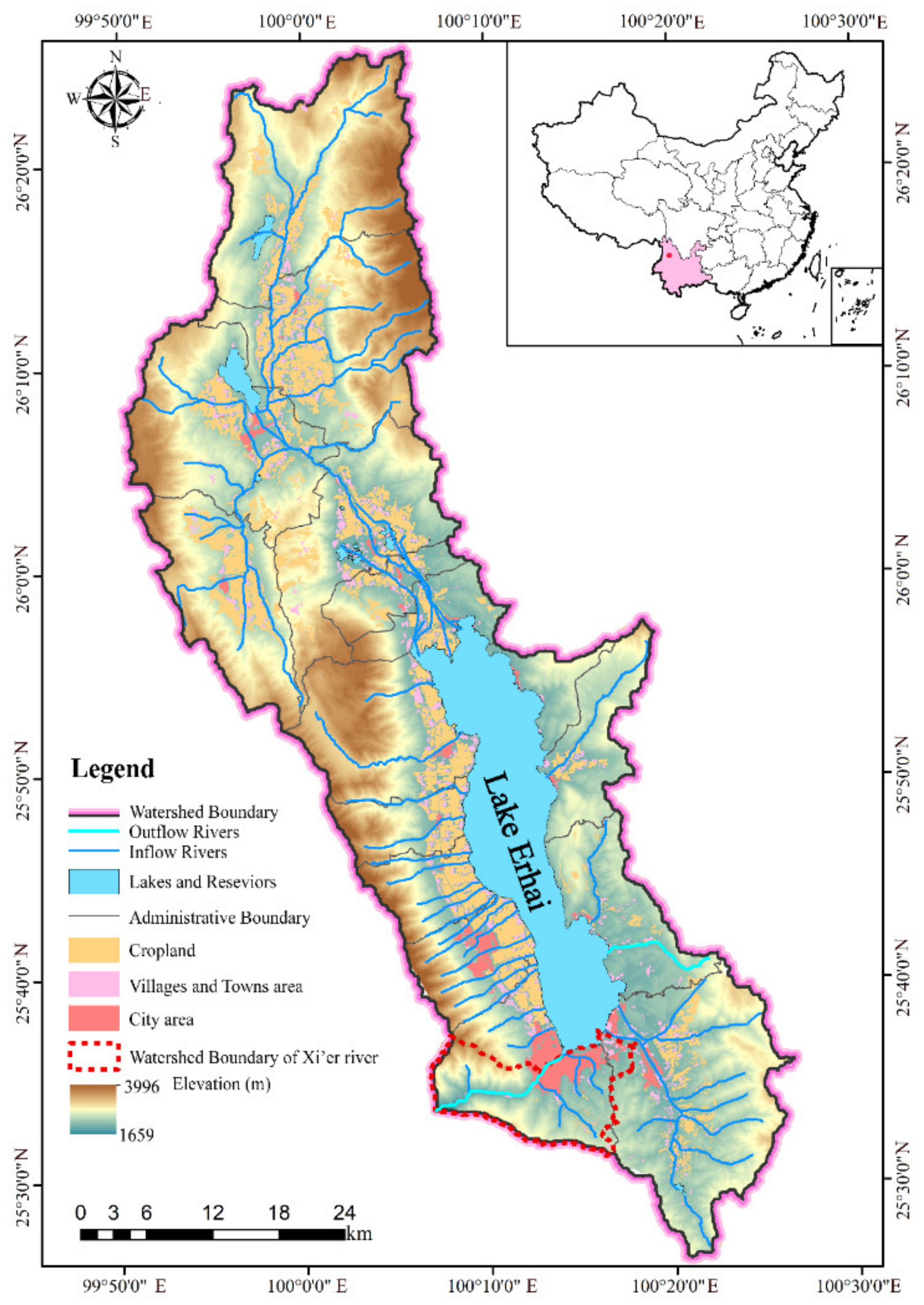
The classic GPP definition is as follows:

$$GPP=\mathrm{NPP}+R$$

(8)

In the single cell, for each time interval, the change in phytoplankton biomass $\Delta B$ is described by the equation below:

$$\frac{\Delta B}{\Delta t}=GPP-R-F$$

(9)

where GPP is the phytoplankton gross primary productivity in a given time interval (g C/m²), R is the time specific rate of total phytoplankton respiration and consumption (including respiration, grazing and settling, g C/m², R is the rate of total phytoplankton respiration and consumption over daily and monthly timescale, when $\Delta t$ = 1 d and 30 d respectively) and F is the time specific rate of phytoplankton moving in or out of the cell by physical transport.

When we calculate the change in phytoplankton biomass for the whole lake, F is generally assumed to be negligible compared with other sources [41]. Thus, the NPP could be estimated in Equation (10) by summarizing the change in total biomass for each time interval.

$$\mathrm{NPP}\left(t\right)=\int \int \int \left(P_{total}\left(t\right)-B{M}_{total}\left(t\right)-P{R}_{total}\left(t\right)\right)dxdydz$$

(10)

where $P_{total}$ is the production rate of all algal group (day⁻¹); $B{M}_{total}$ is the basal metabolism rate of algal group (day⁻¹).

Our study conducted an NPP calculation through the Mass balance Tool and Mass Flux tool in the EFDC Explorer 10.3. These functions allowed the total phytoplankton mass balance and mass flux in the total model’s water columns to be computed based on model output snapshots: the smaller the output snapshot interval, the more accurate the reported results. In our model, the time step was less than 150 s, so in the post-process, we converted the NPP into daily and monthly timescales.

2.2. Study Site

Lake Erhai is a subtropical plateau lake (99°32′–100°27′ E, 25°25′–26°10′ N, 1965.5 m a.s.l), located on the Yunnan-Guizhou Plateau, Southwestern China (Figure 1). The lake’s surface area is approximately 252 km², with a total storage capacity of 29 × 10⁹ m³ and an average depth of 10.8 m. The watershed area is approximately 2565 km². The climate type of Lake Erhai watershed is subtropical, moist monsoon, with a distinctly rainy season (June to September) and dry season (October to March). The annual precipitation of the watershed is 932 mm.

There are 27 major inflows in the north part, west part and south part of the Lake, respectively. Two outlets drain the lake from the south and the east, respectively. In the north, the Muji River system is the largest sub-watershed, covering 61% of the lake watershed [42] and contributing most of the water inflow (50–55% of the total annual inflow) through 3 major rivers (Mijuriver, Yong’an river and Luoshi river). In the west, 18 streams from the Cangshan Mountains are distributed along the narrow coast, constituting important water sources of the lake (40–45% of total annual inflow). The southern water sources of the lake are the Boluo river and the Baita river, supplying an additional 4% of the total annual inflow.

Historically, the water quality of the lake is good and oligotrophic. However, the intensified and imbalanced economic development, rapid urbanization and pressures from anthropogenic activities have significantly impacted this plateau lake, resulting in water quality degradation and eutrophication since the 2000s (Figure S1). The lake water quality experienced a sharp deterioration in 2002–2003. After the explosions of two large algal blooms in 2002 and 2003, the ecosystem shifted greatly from a macrophyte-dominated to an algal-dominated state [43].

2.3. Sample Collection and Analysis

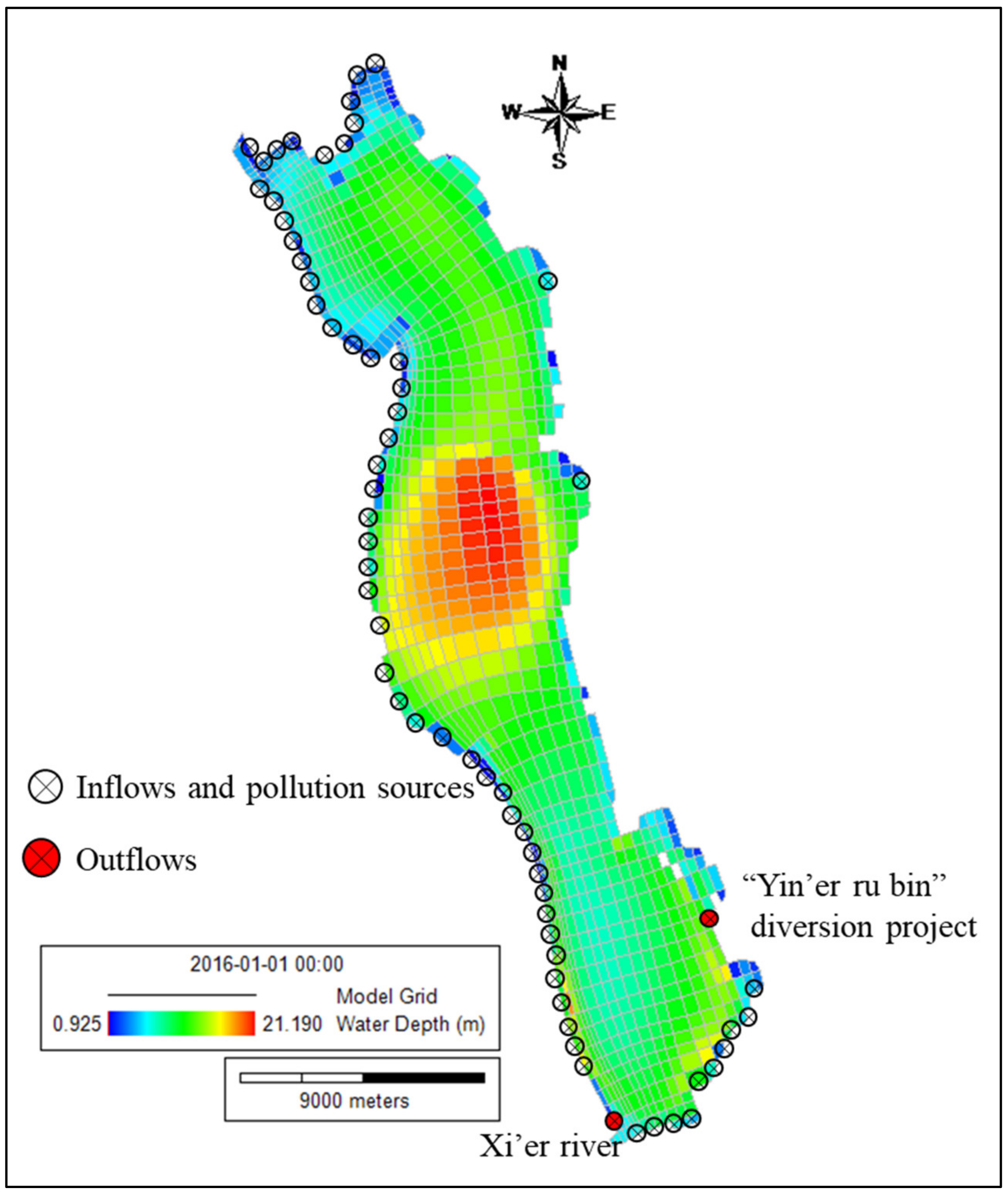
Eleven monitoring sites were designed for monthly routine sampling during 2016 and 2017, water temperature (T) and dissolved oxygen (DO) were measured in situ by using portable instrument (Multi 3420, WTW, Oberbayern, Germany). Samples for total nitrogen (TN), total phosphorus (TP), ammonia nitrogen (NH₄-N), Chla, and phytoplankton biomass measurement were collected in pre-cleaned, acid-washed, brown polyethylene bottles and stored at 4 °C before laboratory analysis. All the chemical parameters were analyzed with three replications following standard methods [44]. Phytoplankton samples were preserved with Lugol’s iodine solution (2% final conc.) and mirror checked. The species of phytoplankton were identified under a microscope (CX21, 400×, Olympus, Tokyo, Japan) based on the protocol in the “Phytoplankton Manual” [45] and “Chinese Freshwater Phytoplankton System, Classification and Ecology” [46]. The algal biomass was calculated based on the cell bio-volume for each species [47]. Additionally, it was converted to biomass in mg C/L based on the carbon content of phytoplankton given by Reynolds et al. [48].

2.4. Model Setup

2.4.1. Grid Generation

The lake was discretized with a curvilinear grid using 1047 grids, in which the most minor grid was approximately 0.26 km², and the largest was approximately 7.4 km². The average depth was 9.98 m, and the deepest grid was approximately 21.2 m in the lake center at the water surface elevation of 1965 m above sea level (Figure 2).

Although there is only weak thermal stratification in Lake Erhai, phytoplankton is still influenced by vertical distribution in light; therefore, it is desirable to resolve variability in vertical light intensity and nutrients using a three-dimensional spatial resolution. In this model, the grid is vertically discretized into five layers, and a total of 5235 computational cells were generated from top to bottom to represent Lake Erhai in its entirety.

2.4.2. Boundary Condition and Nutrient Input

The boundary conditions are the external driving forces of the model. The boundary conditions include the flow rates, water temperature and concentrations of water quality parameters within the inflow tributaries. The flow rates and water quality variables were monitored monthly by the local government of the Ecological and Environmental Bureau of Dali Bai Autonomous Prefecture for major rivers and streams. The boundary conditions were established using these data.

Nutrient loads from non-point pollution were estimated based on local monitoring since 2016 (Figure S2) and a flow balance analysis using the hydrodynamic model. There are nearly 200 agricultural ditches around the lake. These drainage ditches are particularly nutrient rich in the rainy season. Large-scale agricultural non-point pollutants were transported into the lake via these drainage ditches. The flow rates, water temperature, concentration of total nitrogen (TN), total phosphorus (TP) and ammonia–nitrogen (NH₄-N) were measured during the rainy season and dry season, respectively. The yearly nutrient input from the agricultural ditches were calibrated since the loading from ditches could account for 40–50% of the total yearly flux (Figure S3). In the model, we simplified these agricultural drainage ditches as 70 inflows evenly spaced along with the western (40 points), northern (20 points) and southern (10 points) lakeshores (Figure 2). The surface boundary conditions included air temperature, atmospheric pressure, evaporation, precipitation, solar radiation, cloud cover, wind speed and direction on a daily to hourly basis. The meteorological data were sourced from China’s Meteorological Scientific Data Sharing Service Network (http://data.cma.cn/, accessed on 5 December 2021).

Prior research has shown that sediment release in Lake Erhai is mainly triggered by overlying water conditions that vary with the seasons. Sediments can act as a pollutant source for the overlying water [49,50,51]. Thus, we set varied flux rates of PO₄ and ammonia for each season following reported diffusion experiments in the laboratory and in situ measured data [52,53,54].

2.4.3. Model Calibration and Validation

The generated EFDC model needed to be calibrated before it could simulate water quality compliance scenarios and offer quantitative information on the extent of cropping system change. The hydrodynamic module was first calibrated and the daily water elevation and temperature validated. Then, monthly monitoring data from eight sites were selected to calibrate and validate the Lake Erhai water quality simulation (Figure S2). TN, TP, Chla and DO were chosen to carry out the calibration. The calibration procedure was repeated until the simulated values could reproduce the temporal and spatial distributions of observed water quality indexes. The model performance was evaluated by the relative error% (RE%) based on the data of three lake center sites in 2017. The calibrated parameters were given in Appendix A (

Table A1. The model parameters of Lake Erhai EFDC model and calibrated values.

Parameters	Unit	Description	Calibrated Value	Range
Pc	1/day	Maximum growth Rate for Cyanobacteria	1.35	0.2–9.0
Pd	1/day	Maximum growth Rate for Diatoms	0.95	0.2–9.0
Pg	1/day	Maximum growth Rate for Greens	1.7	0.2–9.0
BMc	1/day	Basal Metabolism Rate for Cyanobacteria	0.013	0.01–0.92
BMd	1/day	Basal Metabolism Rate for Diatoms	0.15	0.01–0.92
BMg	1/day	Basal Metabolism Rate for Greens	0.13	0.01–0.92
PRc	1/day	Predation Rate on Cyanobacteria	0.01	0.01–0.06
PRd	1/day	Predation Rate on Diatoms	0.155	0.03–0.3
PRg	1/day	Predation Rate on Greens	0.14	0.03–0.3
Keb	1/m	Background Light Extinction Coefficient	0.38	0.25–0.45
Sc	m/day	Settling velocity for Cyanobacteria	0.02	0.01–0.3
Sd	m/day	Settling velocity for Diatoms	0.12	0.01–0.3
Sg	m/day	Settling velocity for Greens	0.1	0.01–0.3
SRP	m/day	Settling velocity for refractory particulate organic matter (RPOM)	0.05	0.02–9.0
SLP	m/day	Settling velocity for liable particulate organic matter (LPOM)	0.01	0.02–9.0
CChlc	mg C/ug Chl	C:chlorophyll ratio for Cyanobacteria	0.02	0.01–0.05
CChld	mg C/ug Chl	C:chlorophyll ratio for Algae:Diatoms	0.033	0.01–0.05
CChlg	mg C/ug Chl	C:chlorophyll ratio for Algae:Greens	0.033	0.01–0.05
CPprm1		Constant1 used in Determining Algae C:P Ratio (gC/gP)	45	30–65
Keb	1/m	Background Light Extinction Coefficient	0.38	0.15–0.45
KHNc	mg/L	Nitrogen Half-Saturation for Cyanobacteria	0.045	0.01–0.25
KHNd	mg/L	Nitrogen Half-Saturation for Algae:Diatoms	0.05	0.01–0.25
KHNg	mg/L	Nitrogen Half-Saturation for Algae:Greens	0.1	0.01–0.25
KHPc	mg/L	Phosphorus Half-Saturation for Cyanobacteria	0.0033	0.001–0.05
KHPd	mg/L	Phosphorus Half-Saturation for Algae:Diatoms	0.0043	0.001–0.05
KHPg	mg/L	Phosphorus Half-Saturation for Algae:Greens	0.0035	0.001–0.05
TMc1	°C	Lower Optimal Temperature for Growth, Cyanobacteria	23	20–25
TMc2	°C	Upper Optimal Temperature for Growth, Cyanobacteria	30	25–30
TMd1	°C	Lower Optimal Temperature for Growth, Diatoms	10	10–15
TMd2	°C	Upper Optimal Temperature for Growth, Diatoms	22	10–15
TMg1	°C	Lower Optimal Temperature for Growth, Greens	20	22–25
TMg2	°C	Upper Optimal Temperature for Growth, Greens	25	22–26
TMp1	°C	Lower Optimal Temperature for Predation, Diatoms	15	15–25
TMp2	°C	Upper Optimal Temperature for Predation, Diatoms	20	15–26
KTG1c		Suboptimal Temperature Effect Coeff for Growth, Cyanobacteria	0.2	0.001–0.01
KTG2c		Superoptimal Temperature Effect Coeff for Growth, Cyanobacteria	0.03	0.001–0.01
KTG1d		Suboptimal Temperature Effect Coeff for Growth, Diatoms	0.069
KTG2d		Superoptimal Temperature Effect Coeff for Growth, Diatoms	0.1
KTG1g		Suboptimal Temperature Effect Coeff for Growth, Greens	0.1
KTG2g		Superoptimal Temperature Effect Coeff for Growth, Greens	0.01
FNRc		Fraction of Metabolized Nitrogen Produced as RPON, Cyanobacteria	0.15
FNRd		Fraction of Metabolized Nitrogen Produced as RPON, Diatoms	0.15
FNRg		Fraction of Metabolized Nitrogen Produced as RPON, Greens	0.15
FNLc		Fraction of Metabolized Nitrogen Produced as LPON, Cyanobacteria	0.25
FNLd		Fraction of Metabolized Nitrogen Produced as LPON, Diatoms	0.25
FNLg		Fraction of Metabolized Nitrogen Produced as LPON, Greens	0.25
FNDc		Fraction of Metabolized Nitrogen Produced as DON, Cyanobacteria	0.5
FNDd		Fraction of Metabolized Nitrogen Produced as DON, Diatoms	0.5
FNDg		Fraction of Metabolized Nitrogen Produced as DON, Greens	0.5
FNIc		Fraction of Metabolized Nitrogen Produced as DIN, Cyanobacteria	0.1
FNId		Fraction of Metabolized Nitrogen Produced as DIN, Diatoms	0.1
FNIg		Fraction of Metabolized Nitrogen Produced as DIN, Greens	0.1
FPRc		Fraction of Metabolized Phosphorus Produced as RPOP, Cyanobacteria	0
FPRd		Fraction of Metabolized Phosphorus Produced as RPOP, Diatoms	0
FPRg		Fraction of Metabolized Phosphorus Produced as RPOP, Greens	0
FPLc		Fraction of Metabolized Phosphorus Produced as LPOP, Cyanobacteria	0
FPLd		Fraction of Metabolized Phosphorus Produced as LPOP, Diatoms	0
FPLg		Fraction of Metabolized Phosphorus Produced as LPOP, Greens	0
FPDc		Fraction of Metabolized Phosphorus Produced as DOP, Cyanobacteria	0.95
FPDd		Fraction of Metabolized Phosphorus Produced as DOP, Diatoms	0.9
FPDg		Fraction of Metabolized Phosphorus Produced as DOP, Greens	0.9
FPIc		Fraction of Metabolized Phosphorus Produced as P4T, Cyanobacteria	0.05
FPId		Fraction of Metabolized Phosphorus Produced as P4T, Diatoms	0.1
FPIg		Fraction of Metabolized Phosphorus Produced as P4T, Greens	0.1
KRP	1/day	Minimum Hydrolysis Rate of RPOP	0.005	0.001–0.01
KLP	1/day	Minimum Hydrolysis Rate of LPOP	0.005	0.01–0.1
KDP	1/day	Minimum Mineralization Rate of DOP	0.008	0.01–0.3
KRPALG	m3(gc)/d	Constant relating Hydrolysis Rate of RPOP to Algae:	0.005
KLPALG	m3(gc)/d	Constant relating Hydrolysis Rate of LPOP to Algae:	0.01
KDPALG	m3(gc)/d	Constant relating Mineralization Rate of DOP to Algae:	0.01
KRN	1/day	Minimum Hydrolysis Rate of RPON	0.005	0.001–0.01
KLN	1/day	Minimum Hydrolysis Rate of LPON	0.0075	0.01–0.1
KDN	1/day	Minimum Mineralization Rate of DON	0.01	0.01–0.08
KRNALG	m3(gc)−1d−1	Constant relating Hydrolysis Rate of RPON to Algae	0.005	0.0001–0.01
KLNALG	m3(gc)−1d−1	Constant relating Hydrolysis Rate of LPON to Algae	0.005	0.0001–0.02
KDNALG	m3(gc)−1d−1	Constant relating Mineralization Rate of DON to Algae	0.01	0.001–0.01
KHORDO	gO2/m3	oxygen Half-Sat Constant for Algal Respiration	1	0.5–2
KHDNN	gN/m3	half-sat. constant for denitrification	0.001	0.05–0.2
KHCOD	mg/L O2	oxygen half-saturation constant for COD decay	0.7667	1–1.5

The literature range of the parameters are obtained from references [58,63,64,79,80,81,82,83].

)

$$RE\%=\left|\frac{X_i{}^{observed}-X_i{}^{Simulated}}{X_i{}^{observed}}\right|$$

(11)

where $X_i{}^{observed}$ is the observed value of water variables, and $X_i{}^{Simulated}$ is the simulated value of water variables.

2.5. Sensitivity Analysis

To examine the sensitivity of our model, Latin Hypercubic sampling (LHS) combined with distribution-based sensitivity analysis (PAWN) were employed [55]. The selected parameters were first propagated by LHS, and then the output uncertainty was characterized by executing the LHS-created model. Finally, PAWN was used to determine the relative contribution of each parameter to output uncertainties.

The fundamental concept behind the PAWN method is that an input factor’s effect is proportionate to the amount of change in the output distribution caused by correcting that input [56,57]. More specifically, the sensitivity of $y$ to $x_i$ is defined as the difference between the unconditional distribution of $y$ caused by simultaneously varying all input factors and the conditional distribution induced by varying all input factors except $x_i$. The PAWN sensitivity index for the i-th input factor is calculated as follows:

$$KS\left(x_i\right)=\underset{y}{max}|F_y\left(y\right)-F_{y|x_i}\left(\frac{y}{x_i}\right)|$$

(12)

where $F_y\left(y\right)$ and $F_{y|x_i}\left(y/x_i\right)$ are the unconditional and conditional CDFs of $F_{y|x_i}\left(y/x_i\right)$, respectively; y is the output; and stat is a statistic (e.g., maximum, median or mean) defined by the user.

Due to the large number of parameters involved in simulating water quality using EFDC, conducting a global sensitivity analysis on all parameters was computationally prohibitively expensive [58,59]. Therefore, a literature review was conducted to select parameters. To conduct the sensitivity analysis, 21 critical factors relating to phytoplankton growth and sink, as well as the carbon, nitrogen and phosphorus cycles in the aquatic environment, were chosen [60,61,62,63,64,65].

Table 1. Description of parameters for sensitivity analyses.

Parameters	Units	Description	Min	Max
PMc	1/day	Maximum growth rate for cyanobacteria	1.5	2
PMd	1/day	Maximum growth rate for diatom	1.0	2
PMg	1/day	Maximum growth rate for green algae	1.5	2.5
BMRd	1/day	Basal metabolism rate for diatom	0.15	0.3
BMRg	1/day	Basal metabolism rate for green algae	0.06	0.12
PRRd	1/day	Predation rate for diatoms	0.01	0.1
PRRg	1/day	Predation rate for green algae	0.01	0.1
TMc1	°C	Lower optimal temperature for growth of cyanobacteria	20	25
TMc2	°C	Upper optimal temperature for growth of cyanobacteria	26	30
KTG1c	/	Suboptimal temperature effect coefficient for growth of cyanobacteria	0.001	0.01
KHNc	mg/L	Nitrogen half-saturation for cyanobacteria	0.1	0.35
KHPc	mg/L	Phosphorus half-saturation for cyanobacteria	0.0015	0.0025
KHPg	mg/L	Phosphorus half-saturation for phytoplankton:greens	0.002	0.004
WSd	1/day	Settling velocity for diatoms	0.3	0.5
WSrp	1/day	Settling velocity for Refractory particulate organic matter (RPOM)	0.0	0.15
CPprm1	g c/g P	Minimum algae carbon to phosphorus ratio	40	60
rNitM	1/day	Maximum nitrification rate	0.15	0.3
KHNitN	gN/m3	NH4 half-saturation constant for nitrification	0.3	0.8
KHNitDO	gO2/m3	Oxygen half-saturation constant for nitrification	0.5	1
KHORDO	gO2/m3	Oxygen half-saturation constant for algal respiration	1.5	2.5
KDC	1/day	Minimum dissolution rate of dissolved organic carbon (DOC)	0.0015	0.0025

summarizes the ranges of the determined parameters and their descriptions. The LHS sampling and analysis of the output by the PAWN algorithm were performed by using the non-commercial ‘SAFE’ Toolbox in MATLAB [56].

2.6. Statistical Analysis

In the study, Origin 2018 software was used for statistical studies, including calculating mean values, standard deviations, t-tests, Pearson correlation and linear/nonlinear correlations. The spatial distribution of water quality-related factors was obtained using EEMS Explorer 10.3 and ArcGIS 10.2. Linear fitting and t-test results with p < 0.05 are considered significant. Means are given with plus/minus standard deviations.

3. Results and Discussion

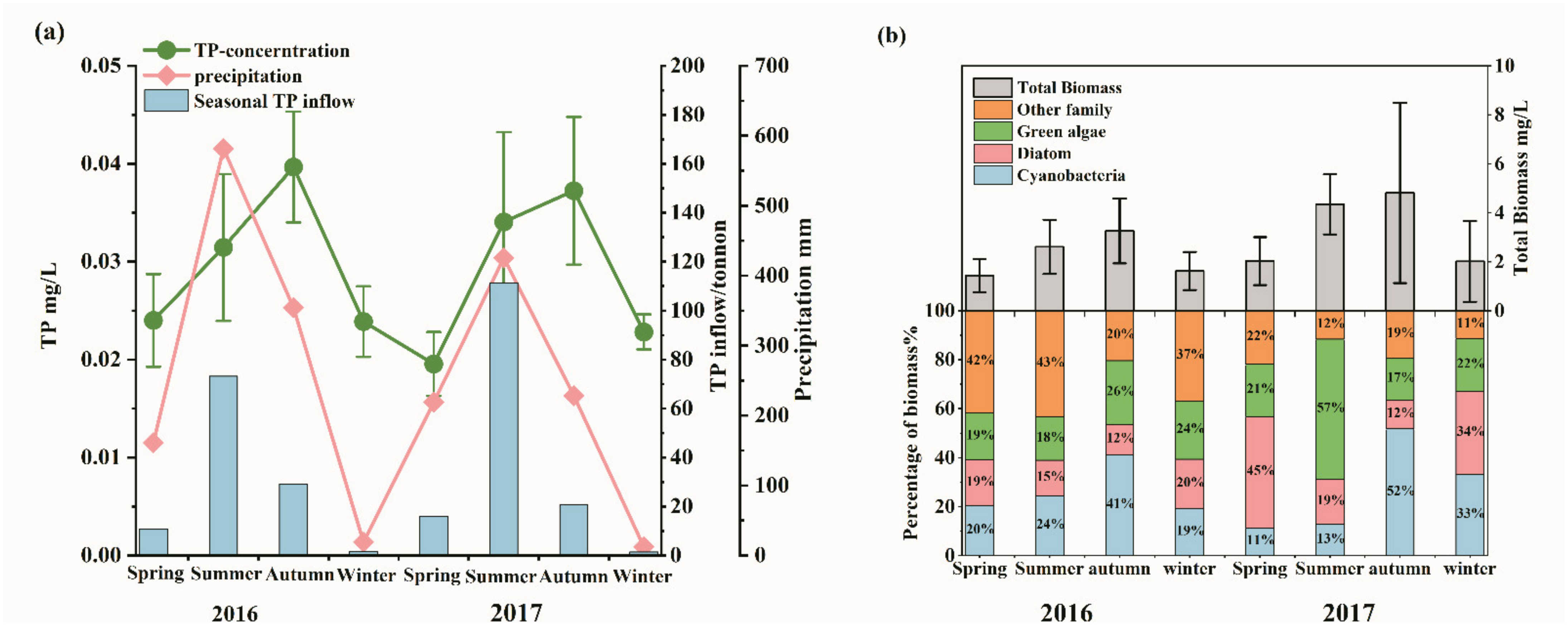
3.1. Seasonal Variation of Phosphorus Load and Algal Biomass

The field investigation revealed clear seasonal changes in external TP loading, TP concentration and total biomass in Lake Erhai. External TP loading was substantially associated with precipitation, with summer inflow accounting for 63% and 74% of the total TP load in 2016 and 2017, respectively. The TP concentration in the lake increased as the TP input increased. The highest value of TP reached 0.057 mg/L in autumn. Then, the TP concentration decreased with the settling of phytoplankton and elevated water level, and the lowest TP was 0.02 mg/L in spring.

The wet algal biomass during 2016–2017 ranged from to 0.41 to 9.97 mg/L, with an average of 2.23 mg/L (Figure 3b). The biomass in the summer (June to August) and autumn (September to November) was significantly higher than that in the spring (March to May) and winter (December to next February). The species compositions of phytoplankton in the lake were mainly diatoms, green algae and cyanobacteria (Figure 3b). The succession of dominance taxa was diatom, green algae and cyanobacteria, representing 45%, 57% and 52% of the total biomass in the spring, summer and autumn of 2017, respectively.

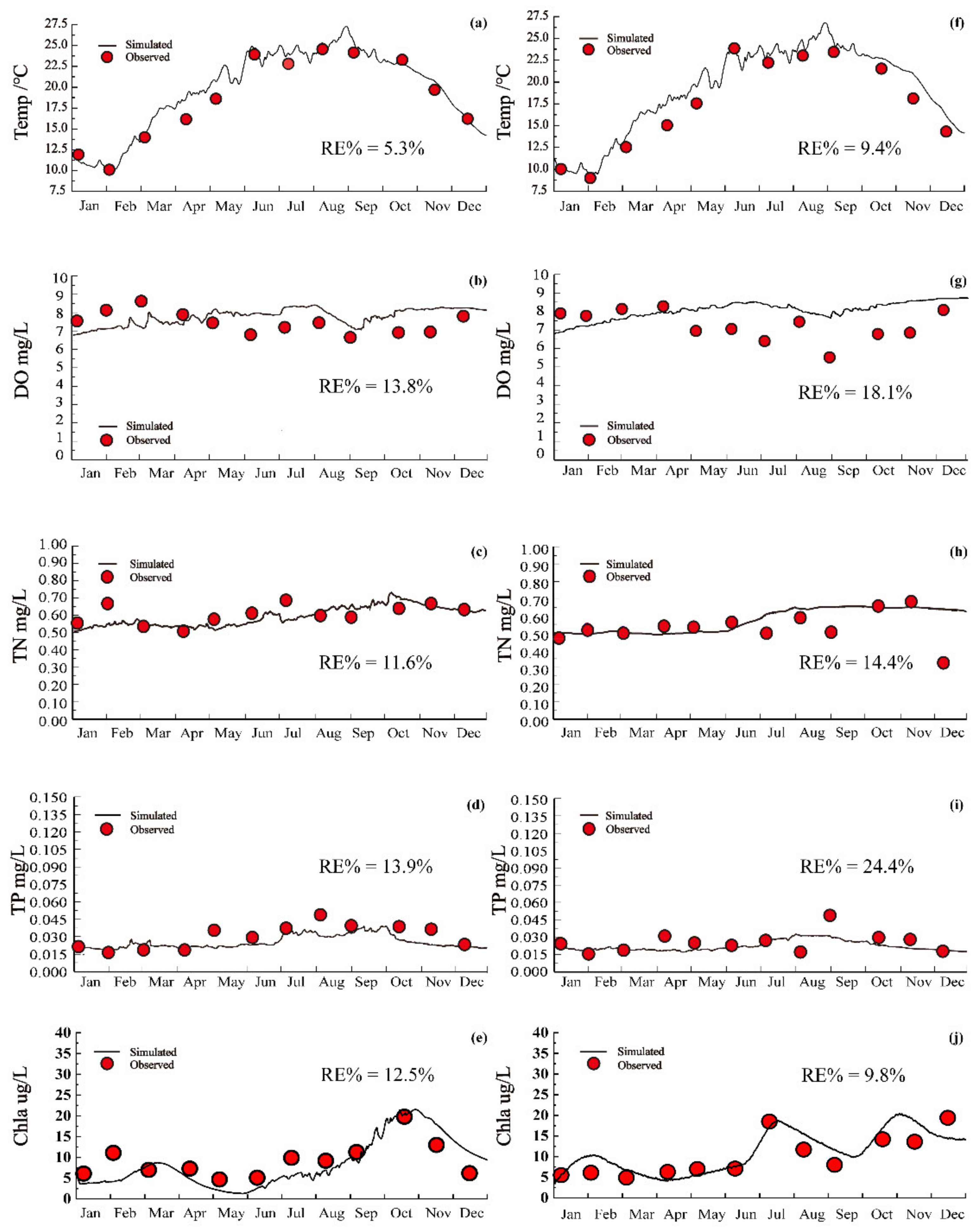
3.2. Model Results with Calibration and Validation

The hydrodynamic simulation of the lake was calibrated through the water level and surface water temperature. The average relative error of the water level simulation and water temperature is 0.3% and 7.74%, respectively, indicating that the established model can accurately reflect the water mass balance and thermodynamic process in the lake (Figure 4a,f and Figure S5). Possible reasons for the error include incomplete data availability, fluctuating water temperature during sampling and sampling errors. Overall, the results of water elevation and temperature simulation showed that the established model performs with sufficient reliability in hydrodynamic and thermodynamic processes.

In terms of water quality and phytoplankton, the simulated concentrations of water quality variables are shown in Figure 4. The average relative errors of TN, TP, Chla and DO of all calibration sites were 12.94, 27.84, 33.72 and 13.96%, respectively. The average relative errors of TN, TP, Chla and DO of 11 validation sites in 2017 were 17.63, 31.82, 36.11 and 17.43%, respectively. Hence, the water quality model developed in this study generally reproduced the variation of water quality over the simulation period, which can be used to analyze the impact of external nutrient load reduction changes on the Lake Erhai water quality.

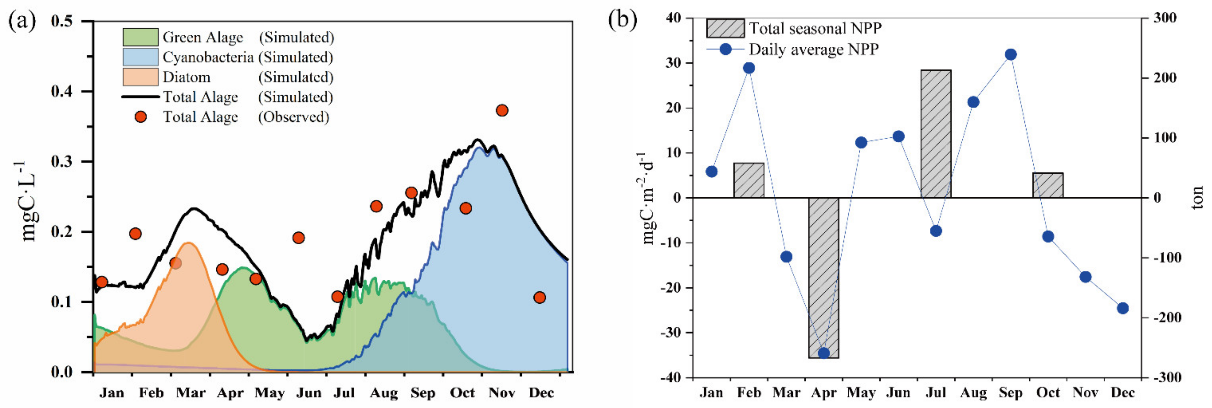
3.3. The Seasonal Dynamic of Phytoplankton Biomass and Net Primary Production

In 2017, the converted algal biomass in Lake Erhai varied between 0.11 and 0.37 mg C/L, with the lowest value occurring in June and the largest value occurring in November. The simulated algal biomass of the model yielded good agreement with the observation. The presence of two peaks corresponds to the massive proliferation of diatom and green algae in spring and the bloom of cyanobacteria in the autumn to winter, respectively. According to Equation (12), the daily, monthly and seasonal net primary production was estimated. The average monthly NPP in 2017 ranged between −34.53 and 31.91 mg C/m²/d and exhibited seasonal congruence. Seasonal fluctuation in total NPP indicates that Lake Erhai is net heterotrophic in spring and net autotrophic in the other three seasons. In summer, the total NPP exceeded 200 t C, which equates to 2500 t in wet weight, approximately. In contrast, the NPP implied a more balanced situation between respiration and growth in autumn and winter. The difference in seasonal NPP can be attributed to the dynamics of the phytoplankton community within the year. In spring, the loss of phytoplankton is primarily related to the grazing and death of diatom, and the decrease in green algae is due to the depletion of bioavailable phosphorus in the lake. In the late summer to autumn, the cyanobacteria became dominant in the lake and thrived as the suitable water temperature and sufficient phosphorus was available. Consequently, the net NPP reached the highest level. In winter, the growth of cyanobacteria was limited by temperature again. The decline in cyanobacteria was the primary cause of negative NPP.

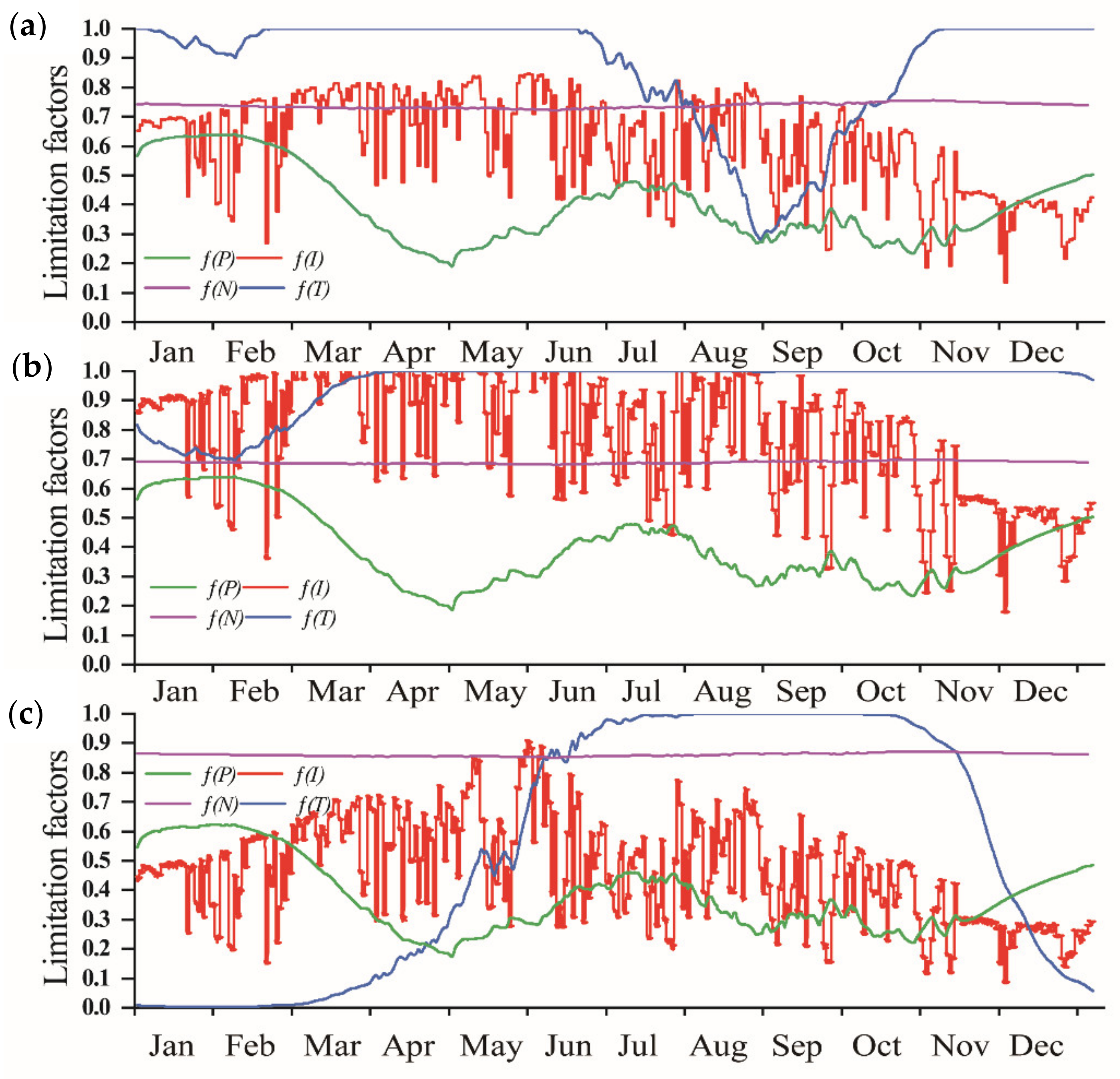
3.4. Limiting Factors of Algal Growth in Erhai

The further analysis of limiting factors of algal growth clearly explains NPP changes within the year. In Figure 5, smaller values of the limiting factor functions indicated the more substantial control of algal growth (i.e., f = 0 means strong limit and f = 1 means no limit) (Figure 6). In Lake Erhai, nitrogen limit factors in the upper water layer (0–1 m below the surface) were more than 0.7 throughout the year, indicating that nitrogen availability does not limit algal growth. In contrast, P restricted the algal growth throughout the year, except in winter. In winter and spring, water temperature limited cyanobacterial growth (limitation function < 0.4), while diatom showed a high primary production and reached the maximum biomass; the production rate of green algae was relatively low, as the temperature also did not favor its growth. They constitute the main parts of the NPP in spring. Then, the phosphorus limitation became stronger from February to May as the settling of diatom gradually exhausted the most bioavailable PO₄ in the surface layer, and external P input was limited in the dry season. The relative growth rate of diatom and green algae decreased to negative. From June to October, when the water temperature reached the optimal growth range of cyanobacteria, it took advantage of quicker phosphorus uptake rates and the buoyancy from gas vesicles, and became dominant in the lake NPP. Finally, in late autumn and winter, the limiting factors gradually changed from P to water temperature again (Figure 6a and Figure 7). Cao et al. [66] also concluded that the pulse of nutrient input after the rainstorm in the summer, together with high temperatures and decreased radiation, was the leading cause of the sustained growth of phytoplankton in the autumn and triggered blooms in favorable meteorological conditions. Generally, water temperature controlled algal growth in Lake Erhai in winter and early spring, while phosphorus had a major impact in summer and autumn.

3.5. Model Sensitivity

The first six most sensitive parameters for the biomass of total phytoplankton communities and three algal groups are listed in

Table 2. The rankings of the first six most influential parameters for Chla concentration (ug/L) and cyanobacteria biomass (CHC), diatom biomass (CHD) and green algae biomass (CHG) derived from the PAWN indices.

Parameters Variables	Rank of Sensitivity
	1	2	3	4	5	6
Total Biomass	KHPg	PRRg	KHPc	PMc	WSrp	PMg
KS value	0.274	0.241	0.212	0.211	0.196	0.188
Biomass (cyanobacteria)	PRRg	KHPg	KHPg	KHPc	PMc	BMRg
KS value	0.292	0.290	0.234	0.212	0.211	0.196
Biomass (diatom)	BMRd	PRRd	PMd	KHNc	KHPc	PRRg
KS value	0.342	0.236	0.230	0.200	0.193	0.192
Biomass (green)	PRRg	BMRd	KHPc	BMRg	KHNc	PMd
KS value	0.275	0.220	0.219	0.214	0.204	0.200

. The parameters were ranked according to their mean Kolmogorov-Smirnov (KS) statistics. Their values are significantly larger than the “dummy sensitivity”, a threshold indicating that this input factor is indeed influential [57].

The total biomass was mainly determined by the utilization capacity of limited resources, precisely, the phosphorus half-saturation concentration and maximum growth rate of green algae and cyanobacteria. Surprisingly, cyanobacteria biomass was strongly influenced by the predation rate and phosphorus half-saturation concentration of green algae. In contrast, the basal metabolism rate of diatom was ranked as the second and third influential parameters on green algae. We attributed this discrepancy to the fact that phytoplankton groups competed against each other by using different strategies of nutrient, light and temperature uptake. Therefore, the results for those phytoplankton groups are sensitive to model parameters that affect their competitive abilities, including growth rate, respiration, predation, and uptake of available nutrients. Diatom, in contrast, was controlled by its rates of respiration, predation and maximum growth rate. A possible reason for this is the different ecological niches other than the two phytoplankton groups.

Moreover, our model simulated the dynamic of phytoplankton biomass and NPP; however, several uncertainties remain in the model. The first arises from a significant lack of actual monitoring data of NPP to calculate and verify our model, as only Chla concentration and biomass data could be collected from the monitoring data. We were constrained to assuming that the GPP data obtained from the literature represent the annual average concentration. This was still not sufficient to build an accurate model.

The second arises from the uncertainties of boundary conditions, especially the measure and estimation of the nutrient from cropland via runoff to rivers and ditches. In addition, there is incongruence between the classification of water quality variables from lab water analysis and the EFDC model. We had to estimate the proportion of refractory and liable organic components in particulate nitrogen/phosphorus using empirical conversion factors.

Furthermore, the complex and incompletely understood ecological mechanisms underlying phytoplankton community dynamics, such as growth rate, resource competition, grazing rate and the inherent plasticity of the organism C: N: P stoichiometry, may lead to bias in the predictions of the community’s response to external changes as a result of the model’s intrinsic structure. For example, Yu et al. [67] reported that the bloom-forming cyanobacteria in Lake Erhai include seven Microcystis, four Dolichospermum and two Aphanizomenon species. The coexistence of N₂-fixer and non-N₂-fixer, as well as various strategies in nitrogen and phosphorus competition, increased the uncertainties and challenges of the mechanistic model in reproducing algal dynamics and Chla concentration during the high-risk period [68]. The parameters in our analysis are consistent for the whole lake. Some optimization approaches, such as employing time- and space-varying parameters, have succeeded in improving the simulation accuracy [62,69]. These are the issues that should be addressed in our future research.

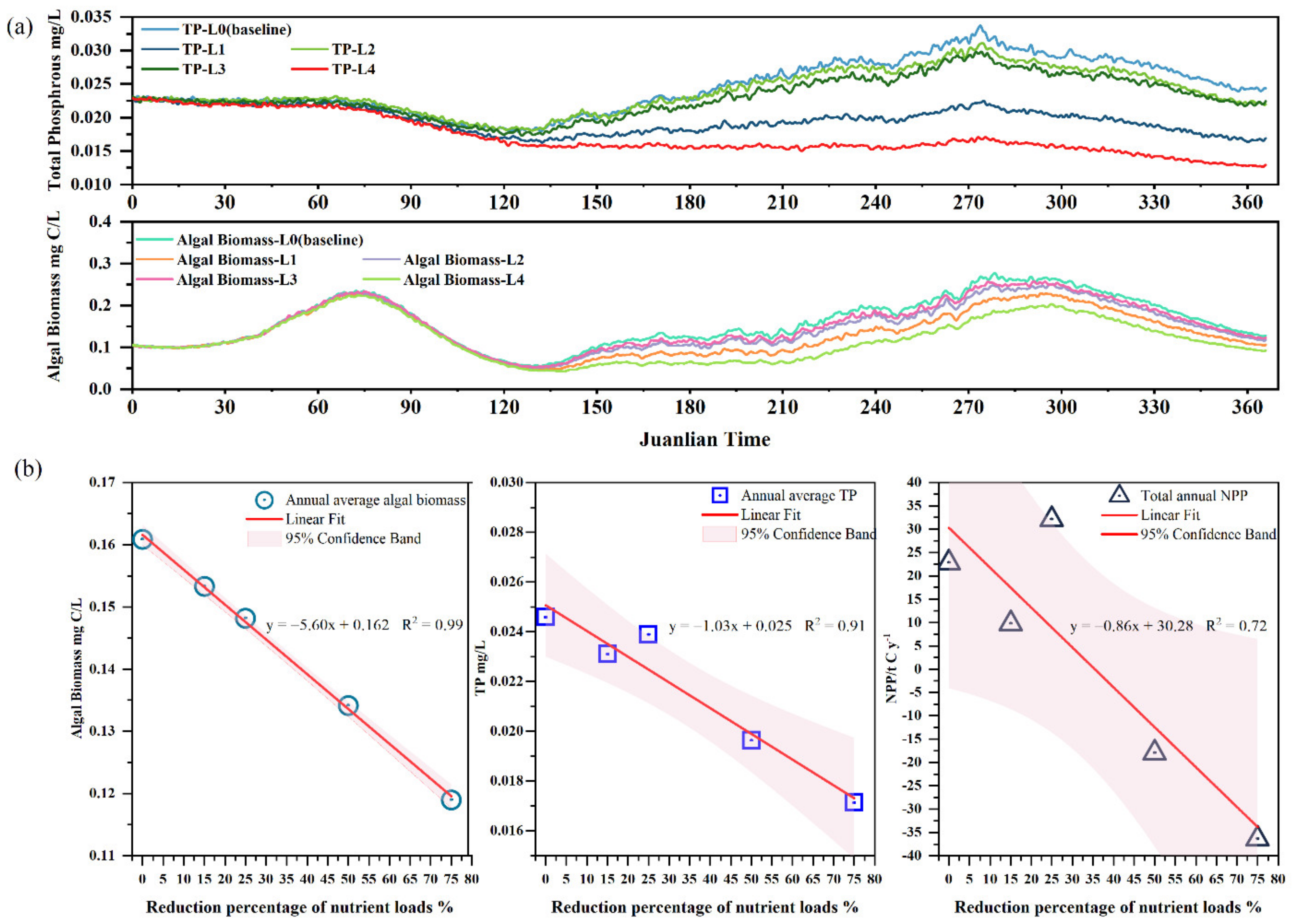
3.6. Response of NPP to the Phosphorous Load Reduction

The results of our model indicate that the water quality of Lake Erhai would not be able to attain the targeted water quality standards (maintain <0.025 mg/L (Class II) for the whole year) under current watershed TP loading. It is necessary to provide reasonable predictions required for nutrient management in the lake. Accordingly, we designed four scenarios with the phosphorus reduced by 15% to 75% to evaluate the effect on TP concentration in the lake and phytoplankton production (

Table 3. Four reduction scenarios under the existing watershed loading conditions.

	Loading Reduction Ratio	Reduction in TP t/a
L0	/	0
L1	15% reduction in TP	22.35
L2	25% reduction in TP	37.25
L3	50% reduction in TP	74.5
L4	75% reduction and TP	111.8

).

The time series plot of the four scenarios is illustrated in Figure 7. The results showed that the annual average concentrations decreased by 5, 8, 17 and 26% for algal biomass, and 3, 6, 20 and 30% for TP, respectively. Due to the fact that the majority of phosphorus input occurred during the summer, the algal biomass and TP concentration in spring were not significantly affected by load reduction, and the difference in NPP between the scenarios was negligible. In summer and autumn, the NPP steadily decreased with the increase in the load reduction ratio.

Based on the modeled results, we analyzed the relationship between the reduction and change in algal biomass, TP and NPP. As illustrated in Figure 7b, the average biomass and TP concentration are linearly related to loading reduction percentage. It can be concluded that phosphorus loading reduction directly affects the water quality of Lake Erhai, and the efficiency of improvement is proportionate to the degree of load decrease, which implied that external loads contribute most to variations in net algal growth in Lake Erhai, while other factors, such as meteorological conditions and physical transport, play a less significant role [70,71,72]. Based on load–response curves, it is possible to determine the required load of phosphorus in order to reach a desired level of eutrophication. Considering the relative error of our model, TP loads from influent tributaries and agriculture ditches of Lake Erhai would have to be reduced by at least 25% to enable the water quality to reach Grade II for TP.

Meanwhile, reduced phosphorus further restrained the growth of phytoplankton and led to decreased annual NPP. As predicted by our model, the yearly production/biomass ratio (e.g., kg produced per year per kg biomass) of lake Erhai will less than 1 when the inflow TP concentration is reduced by 45%. These results are helpful for the mitigation of eutrophication. Recent investigations indicated that Lake Erhai had undergone a transition from the mesotrophic to the preliminary stages of the eutrophic state [73], implying that its current environmental carrying capacity is quite limited. There will be great challenges associated with remediating the aquatic environment through intensive restoration activities if the transition of ecological status and new ecological stability are reached [74,75,76] Therefore, controlling the lake’s NPP is critical for the protection of Lake Erhai.

4. Conclusions

• A 3D hydrodynamic and water quality model was developed for Lake Erhai, China. In the field investigation, the water surface elevation, temperature, nutrients and algal biomass concentration in the lake were accurately simulated by the numerical model, revealing a reasonable picture of the lake’s hydrodynamics and eutrophication process. The model is suitable to calculate the seasonal NPP in the lake.
• According to the modeling results, the average daily NPP ranged from −3.45 and 3.19 mg C/m²/d. The seasonal fluctuation in total NPP indicates that Lake Erhai is net heterotrophic in spring and net autotrophic in summer, autumn, and winter. The difference in seasonal NPP can be attributed to the combined impact of phosphorus supply and temperature limitation of the phytoplankton community within the year.
• The results of loading reduction scenarios indicate that phosphorus loading reduction directly affects the water quality of Lake Erhai, and the efficiency of improvement in TP concentration and NPP is proportionate to the degree of load decrease.

References

1. Pomati, F.; Matthews, B.; Seehausen, O.; Ibelings, B.W. Eutrophication and Climate Warming Alter Spatial (Depth) Co-Occurrence Patterns of Lake Phytoplankton Assemblages. Hydrobiologia 2017, 787, 375–385. [Google Scholar] [CrossRef]
2. Wells, M.L.; Trainer, V.L.; Smayda, T.J.; Karlson, B.S.O.; Trick, C.G.; Kudela, R.M.; Ishikawa, A.; Bernard, S.; Wulff, A.; Anderson, D.M.; et al. Harmful Algal Blooms and Climate Change: Learning from the Past and Present to Forecast the Future. Harmful Algae 2015, 49, 68–93. [Google Scholar] [CrossRef] [PubMed] [Green Version]
3. Le Moal, M.; Gascuel-Odoux, C.; Ménesguen, A.; Souchon, Y.; Étrillard, C.; Levain, A.; Moatar, F.; Pannard, A.; Souchu, P.; Lefebvre, A.; et al. Eutrophication: A New Wine in an Old Bottle? Sci. Total Environ. 2019, 651, 1–11. [Google Scholar] [CrossRef] [Green Version]
4. Goyette, J.O.; Bennett, E.M.; Maranger, R. Low Buffering Capacity and Slow Recovery of Anthropogenic Phosphorus Pollution in Watersheds. Nat. Geosci. 2018, 11, 921–925. [Google Scholar] [CrossRef]
5. Schurz, C.; Hollosi, B.; Matulla, C.; Pressl, A.; Ertl, T.; Schulz, K.; Mehdi, B. A Comprehensive Sensitivity and Uncertainty Analysis for Discharge and Nitrate-Nitrogen Loads Involving Multiple Discrete Model Inputs under Future Changing Conditions. Hydrol. Earth Syst. Sci. 2019, 23, 1211–1244. [Google Scholar] [CrossRef] [Green Version]
6. Tong, Y.; Zhang, W.; Wang, X.; Couture, R.M.; Larssen, T.; Zhao, Y.; Li, J.; Liang, H.; Liu, X.; Bu, X.; et al. Decline in Chinese Lake Phosphorus Concentration Accompanied by Shift in Sources since 2006. Nat. Geosci. 2017, 10, 507–511. [Google Scholar] [CrossRef]
7. Gao, Y.; Jia, J.; Lu, Y.; Yang, T.; Lyu, S.; Shi, K.; Zhou, F.; Yu, G. Determining Dominating Control Mechanisms of Inland Water Carbon Cycling Processes and Associated Gross Primary Productivity on Regional and Global Scales. Earth Sci. Rev. 2021, 213, 103497. [Google Scholar] [CrossRef]
8. López-Sandoval, D.C.; Duarte, C.M.; Agustí, S. Nutrient and Temperature Constraints on Primary Production and Net Phytoplankton Growth in a Tropical Ecosystem. Limnol. Oceanogr. 2021, 66, 2923–2935. [Google Scholar] [CrossRef]
9. Trochine, C.; Guerrieri, M.E.; Liboriussen, L.; Lauridsen, T.L.; Jeppesen, E. Effects of Nutrient Loading, Temperature Regime and Grazing Pressure on Nutrient Limitation of Periphyton in Experimental Ponds. Freshw. Biol. 2014, 59, 905–917. [Google Scholar] [CrossRef]
10. Val, J.; Pino, R.; Navarro, E.; Chinarro, D. Addressing the Local Aspects of Global Change Impacts on Stream Metabolism Using Frequency Analysis Tools. Sci. Total Environ. 2016, 569–570, 798–814. [Google Scholar] [CrossRef]
11. Genzoli, L.; Hall, R.O., Jr. Shifts in Klamath River Metabolism Following a Reservoir Cyanobacterial Bloom. Freshw. Sci. 2016, 35, 795–809. [Google Scholar] [CrossRef]
12. Kuehl, L.C.; Troelstrup, N.H., Jr. Relationships between Net Primary Reproduction, Water Transparency, Chlorophyll a, and Total Phosphorous in Oak Lake, Brookings County, South Dakota. Proc. S. D. Acad. Sci. 2013, 92, 67–78. [Google Scholar]
13. Kemp, W.M.; Smith, E.M.; Marvin-DiPasquale, M.; Boynton, W.R. Organic Carbon Balance and Net Ecosystem Metabolism in Chesapeake Bay. Mar. Ecol. Prog. Ser. 1997, 150, 229–248. [Google Scholar] [CrossRef]
14. Gazeau, F.; Borges, A.V.; Barrón, C.; Duarte, C.M.; Iversen, N.; Middelburg, J.J.; Delille, B.; Pizay, M.D.; Frankignoulle, M.; Gattuso, J.P. Net Ecosystem Metabolism in a Micro-Tidal Estuary (Randers Fjord, Denmark): Evaluation of Methods. Mar. Ecol. Prog. Ser. 2005, 301, 23–41. [Google Scholar] [CrossRef]
15. Staehr, P.A.; Bade, D.; van de Bogert, M.C.; Koch, G.R.; Williamson, C.; Hanson, P.; Cole, J.J.; Kratz, T. Lake Metabolism and the Diel Oxygen Technique: State of the Science. Limnol. Oceanogr. Methods 2010, 8, 628–644. [Google Scholar] [CrossRef]
16. Gelda, R.K.; Effler, S.W. Metabolic Rate Estimates for a Eutrophic Lake from Diel Dissolved Oxygen Signals. Hydrobiologia 2002, 485, 51–66. [Google Scholar] [CrossRef]
17. Caffrey, J.M. Production, Respiration and Net Ecosystem Metabolism U.S. Estuaries. Environ. Monit. Assess. 2003, 81, 207–219. [Google Scholar] [CrossRef]
18. Quay, P.D.; Wilbur, D.; Richey, J.E.; Devol, A.H.; Benner, R.; Forsberg, B.R. The 18O:16O of Dissolved Oxygen in Rivers and Lakes in the Amazon Basin: Determining the Ratio of Respiration to Photosynthesis Rates in Freshwaters. Limnol. Oceanogr. 1995, 40, 718–729. [Google Scholar] [CrossRef]
19. Tobias, C.R.; Böhlke, J.K.; Harvey, J.W. The Oxygen-18 Isotope Approach for Measuring Aquatic Metabolism in High-Productivity Waters. Limnol. Oceanogr. 2007, 52, 1439–1453. [Google Scholar] [CrossRef]
20. Hamilton, D.P.; Schladow, S.G. Prediction of Water Quality in Lakes and Reservoirs. Part I—Model Description. Ecol. Model. 1997, 96, 91–110. [Google Scholar] [CrossRef]
21. Schladow, S.G.; Hamilton, D.P. Prediction of Water Quality in Lakes and Reservoirs: Part II—Model Calibration, Sensitivity Analysis and Application. Ecol. Model. 1997, 96, 111–123. [Google Scholar] [CrossRef]
22. Riley, M.J.; Stefan, H.G. Development of the Minnesota Lake Water Quality Management Model “Minlake”. Lake Reserv. Manag. 1988, 4, 73–83. [Google Scholar] [CrossRef] [Green Version]
23. Cloern, J.E. The Relative Importance of Light and Nutrient Limitation of Phytoplankton Growth: A Simple Index of Coastal Ecosystem Sensitivity to Nutrient Enrichment. Aquat. Ecol. 1999, 33, 3–15. [Google Scholar] [CrossRef]
24. Mortazavi, B.; Iverson, R.L.; Landing, W.M.; Lewis, F.G.; Huang, W. Control of Phytoplankton Production and Biomass in a River-Dominated Estuary: Apalachicola Bay, Florida, USA. Mar. Ecol. Prog. Ser. 2000, 198, 19–31. [Google Scholar] [CrossRef]
25. Muylaert, K.; Tackx, M.; Vyverman, W. Phytoplankton Growth Rates in the Freshwater Tidal Reaches of the Schelde Estuary (Belgium) Estimated Using a Simple Light-Limited Primary Production Model. Hydrobiologia 2005, 540, 127–140. [Google Scholar] [CrossRef]
26. Pinckney, J.L.; Paerl, H.W.; Harrington, M.B. Responses of the Phytoplankton Community Growth Rate to Nutrient Pulses in Variable Estuarine Environments. J. Phycol. 1999, 35, 1455–1463. [Google Scholar] [CrossRef]
27. Strock, J.P.; Menden-Deuer, S. Temperature Acclimation Alters Phytoplankton Growth and Production Rates. Limnol. Oceanogr. 2021, 66, 740–752. [Google Scholar] [CrossRef]
28. Klausmeier, C.A.; Litchman, E.; Levin, S.A. Phytoplankton Growth and Stoichiometry under Multiple Nutrient Limitation. Limnol. Oceanogr. 2004, 49, 1463–1470. [Google Scholar] [CrossRef] [Green Version]
29. Azevedo, I.C.; Bordalo, A.A.; Duarte, P.M. Influence of River Discharge Patterns on the Hydrodynamics and Potential Contaminant Dispersion in the Douro Estuary (Portugal). Water Res. 2010, 44, 3133–3146. [Google Scholar] [CrossRef]
30. Azevedo, I.C.; Bordalo, A.A.; Duarte, P. Influence of Freshwater Inflow Variability on the Douro Estuary Primary Productivity: A Modelling Study. Ecol. Model. 2014, 272, 1–15. [Google Scholar] [CrossRef]
31. Yan, J.; Liu, J.; You, X.; Shi, X.; Zhang, L. Simulating the Gross Primary Production and Ecosystem Respiration of Estuarine Ecosystem in North China with AQUATOX. Ecol. Model. 2018, 373, 1–12. [Google Scholar] [CrossRef]
32. Hamrick, J.M. A Three-Dimensional Environmental Fluid Dynamics Computer Code: Theoretical and Computational Aspects; Virginia Institute of Marine Science: Gloucester Point, VA, USA, 1992. [Google Scholar]
33. Qin, Q.; Shen, J. The Contribution of Local and Transport Processes to Phytoplankton Biomass Variability over Different Timescales in the Upper James River, Virginia. Estuar. Coast. Shelf Sci. 2017, 196, 123–133. [Google Scholar] [CrossRef] [Green Version]
34. Camacho, R.A.; Martin, J.L.; Watson, B.; Paul, M.J.; Zheng, L.; Stribling, J.B. Modeling the Factors Controlling Phytoplankton in the St. Louis Bay Estuary, Mississippi and Evaluating Estuarine Responses to Nutrient Load Modifications. J. Environ. Eng. 2015, 141, 04014067. [Google Scholar] [CrossRef]
35. Rong, Z.; Huan, W.; Dezhao, Y.; Cheng, Z.; Hong, S.; Jun, C. Dynamic Changes of Microcystins and Phytoplankton during the Cyanobacterial Bloom in Lake Erhai in 2013. J. Lake Sci. 2015, 27, 378–384. [Google Scholar] [CrossRef]
36. Turner, M.A.; Sigurdson, L.J.; Findlay, D.L.; Howell, E.T.; Robinson, G.G.C.; Brewster, J.F. Growth Characteristics of Bloom-Forming Filamentous Green Algae in the Littoral Zone of an Experimentally Acidified Lake. Can. J. Fish. Aquat. Sci. 1995, 52, 2251–2263. [Google Scholar] [CrossRef]
37. Xiao, M.; Willis, A.; Burford, M.A. Differences in Cyanobacterial Strain Responses to Light and Temperature Reflect Species Plasticity. Harmful Algae 2017, 62, 84–93. [Google Scholar] [CrossRef] [Green Version]
38. Liu, X.; Lu, X.; Chen, Y. The Effects of Temperature and Nutrient Ratios on Microcystis Blooms in Lake Taihu, China: An 11-Year Investigation. Harmful Algae 2011, 10, 337–343. [Google Scholar] [CrossRef]
39. Cerco, C.F.; Cole, T.M. Three-Dimensional Eutrophication Model of Chesapeake Bay. Volume 1: Main Report; Final Report; FAO: Rome, Italy, 2006. [Google Scholar]
40. Park, K.; Kuo, A.Y.; Shen, J.; Hamrick, J.M. A Three-Dimensional Hydrodyamic-Eutrophication Model (HEM-3D): Description of Water Quality and Sediment Process Submodels (EFDC Water Quality Model); William & Mary: Williamsburg, VA, USA, 1995; p. 327. [Google Scholar]
41. Odum, H.T. Primary Production in Flowing Waters. Limnol. Oceanogr. 1956, 1, 102–117. [Google Scholar] [CrossRef]
42. Wang, S.; Zhang, L.; Ni, L.; Zhao, H.; Jiao, L.; Yang, S.; Guo, L.; Shen, J. Ecological Degeneration of the Erhai Lake and Prevention Measures. Environ. Earth Sci. 2015, 74, 3839–3847. [Google Scholar] [CrossRef]
43. Zhang, L.; Xu, K.; Wang, S.; Wang, S.; Li, Y.; Li, Q.; Meng, Z. Characteristics of Dissolved Organic Nitrogen in Overlying Water of Typical Lakes of Yunnan Plateau. China. Ecol. Indic. 2017, 84, 727–737. [Google Scholar] [CrossRef]
44. American Public Health Association (APHA). Standard Methods for the Examination of Water and Wastewater, 21st ed.; APHA: Washington, DC, USA, 2005. [Google Scholar]
45. Hasle, G.R.; Sournia, A. Phytoplankton Manual, Monographs on Oceanographic Methodology. In Concentrating Phytoplankton. Settling. The Inverted Microscope Method; Unesco: Paris, France, 1978. [Google Scholar]
46. Hu, H. The Freshwater Algae of China: Systematics, Taxonomy and Ecology; Science Press: Beijing, China, 2006; ISBN 7030166337. [Google Scholar]
47. Sun, J.; Liu, D. Study on Phytoplankton Biomass I. Phytoplankton Measurement Biomass from Cell Volume or Plasma Volume. Acta Oceanol. Sin. 1999, 21, 75–85. [Google Scholar]
48. Reynolds, C.S. The Ecology of Phytoplankton; Cambridge University Press: Cambridge, UK, 2006; ISBN 1139454897. [Google Scholar]
49. Spears, B.M.; Carvalho, L.; Perkins, R.; Kirika, A.; Paterson, D.M. Sediment Phosphorus Cycling in a Large Shallow Lake: Spatio-Temporal Variation in Phosphorus Pools and Release. Hydrobiologia 2007, 584, 37–48. [Google Scholar] [CrossRef]
50. Zou, R.; Wu, Z.; Zhao, L.; Elser, J.J.; Yu, Y.; Chen, Y.; Liu, Y. Seasonal Algal Blooms Support Sediment Release of Phosphorus via Positive Feedback in a Eutrophic Lake: Insights from a Nutrient Flux Tracking Modeling. Ecol. Model. 2020, 416, 108881. [Google Scholar] [CrossRef]
51. Fan, P.; Wang, Y.; Wang, W.; Chai, B.; Lu, X.; Zhao, J.; Fan, P.; Wang, W.; Lu, X. Release Characteristics of Nitrogen and Phosphorus from Sediments Formed under Different Supplemental Water Sources in Xi’an Moat, China. Environ. Sci. Pollut. Res. 2019, 26, 10746–10755. [Google Scholar] [CrossRef] [PubMed]
52. Zhao, H.; Zhang, L.; Wang, S.; Jiao, L. Features and Influencing Factors of Nitrogen and Phosphorus Diffusive Fluxes at the Sediment-Water Interface of Erhai Lake. Environ. Sci. Pollut. Res. 2018, 25, 1933–1942. [Google Scholar] [CrossRef] [PubMed]
53. Pan, X.; Lin, L.; Huang, Z.; Liu, M.; Dong, L.; Chen, J.; Crittenden, J. Distribution Characteristics and Pollution Risk Evaluation of the Nitrogen and Phosphorus Species in the Sediments of Lake Erhai, Southwest China. Environ. Sci. Pollut. Res. 2019, 26, 22295–22304. [Google Scholar] [CrossRef]
54. Ni, Z.; Wang, S. Historical Accumulation and Environmental Risk of Nitrogen and Phosphorus in Sediments of Erhai Lake, Southwest China. Ecol. Eng. 2015, 79, 42–53. [Google Scholar] [CrossRef]
55. Chaturvedi, S.; Rajasekar, E. Application of a Probabilistic LHS-PAWN Approach to Assess Building Cooling Energy Demand Uncertainties. Build. Simul. 2022, 15, 373–387. [Google Scholar] [CrossRef]
56. Pianosi, F.; Wagener, T. A Simple and Efficient Method for Global Sensitivity Analysis Based On Cumulative Distribution Functions. Environ. Model. Softw. 2015, 67, 1–11. [Google Scholar] [CrossRef] [Green Version]
57. Pianosi, F.; Wagener, T. Distribution-Based Sensitivity Analysis from a Generic Input-Output Sample. Environ. Model. Softw. 2018, 108, 197–207. [Google Scholar] [CrossRef] [Green Version]
58. Muleta, M.K.; Nicklow, J.W. Sensitivity and Uncertainty Analysis Coupled with Automatic Calibration for a Distributed Watershed Model. J. Hydrol. 2005, 306, 127–145. [Google Scholar] [CrossRef] [Green Version]
59. Campolongo, F.; Cariboni, J.; Saltelli, A. An Effective Screening Design for Sensitivity Analysis of Large Models. Environ. Model. Softw. 2007, 22, 1509–1518. [Google Scholar] [CrossRef]
60. Tang, T.J.; Yang, S.; Peng, Y.; Yin, K.; Zou, R. Eutrophication Control Decision Making Using EFDC Model for Shenzhen Reservoir, China. Water Resour. 2017, 44, 308–314. [Google Scholar] [CrossRef]
61. Wu, G.; Xu, Z. Prediction of Algal Blooming Using EFDC Model: Case Study in the Daoxiang Lake. Ecol. Model. 2011, 222, 1245–1252. [Google Scholar] [CrossRef]
62. Kim, J.; Lee, T.; Seo, D. Algal Bloom Prediction of the Lower Han River, Korea Using the EFDC Hydrodynamic and Water Quality Model. Ecol. Model. 2017, 366, 27–36. [Google Scholar] [CrossRef]
63. Yi, X.; Zou, R.; Guo, H. Global Sensitivity Analysis of a Three-Dimensional Nutrients-Algae Dynamic Model for a Large Shallow Lake. Ecol. Model. 2016, 327, 74–84. [Google Scholar] [CrossRef]
64. Arhonditsis, G.B.; Brett, M.T. Eutrophication Model for Lake Washington (USA): Part I. Model Description and Sensitivity Analysis. Ecol. Model. 2005, 187, 140–178. [Google Scholar] [CrossRef]
65. Jiang, L.; Li, Y.; Zhao, X.; Tillotson, M.R.; Wang, W.; Zhang, S.; Sarpong, L.; Asmaa, Q.; Pan, B. Parameter Uncertainty and Sensitivity Analysis of Water Quality Model in Lake Taihu, China. Ecol. Model. 2018, 375, 1–12. [Google Scholar] [CrossRef]
66. Cao, J.; Hou, Z.; Li, Z.; Chu, Z.; Yang, P.; Zheng, B. Succession of Phytoplankton Functional Groups and Their Driving Factors in a Subtropical Plateau Lake. Sci. Total Environ. 2018, 631–632, 1127–1137. [Google Scholar] [CrossRef]
67. Yu, G.; Jiang, Y.; Song, G.; Tan, W.; Zhu, M.; Li, R. Variation of Microcystis and Microcystins Coupling Nitrogen and Phosphorus Nutrients in Lake Erhai, a Drinking-Water Source in Southwest Plateau, China. Environ. Sci. Pollut. Res. 2014, 21, 9887–9898. [Google Scholar] [CrossRef]
68. Nelson, N.G.; Muñoz-Carpena, R.; Phlips, E. Parameter Uncertainty Drives Important Incongruities between Simulated Chlorophyll-a and Phytoplankton Functional Group Dynamics in a Mechanistic Management Model. Environ. Model. Softw. 2020, 129, 104708. [Google Scholar] [CrossRef]
69. Sadeghian, A.; Chapra, S.C.; Hudson, J.; Wheater, H.; Lindenschmidt, K.E. Improving In-Lake Water Quality Modeling Using Variable Chlorophyll a/Algal Biomass Ratios. Environ. Model. Softw. 2018, 101, 73–85. [Google Scholar] [CrossRef]
70. Scavia, D.; David Allan, J.; Arend, K.K.; Bartell, S.; Beletsky, D.; Bosch, N.S.; Brandt, S.B.; Briland, R.D.; Daloğlu, I.; DePinto, J.V.; et al. Assessing and Addressing the Re-Eutrophication of Lake Erie: Central Basin Hypoxia. J. Great Lakes Res. 2014, 40, 226–246. [Google Scholar] [CrossRef]
71. Bertani, I.; Obenour, D.R.; Steger, C.E.; Stow, C.A.; Gronewold, A.D.; Scavia, D. Probabilistically Assessing the Role of Nutrient Loading in Harmful Algal Bloom Formation in Western Lake Erie. J. Great Lakes Res. 2016, 42, 1184–1192. [Google Scholar] [CrossRef] [Green Version]
72. Rucinski, D.K.; DePinto, J.V.; Beletsky, D.; Scavia, D. Modeling Hypoxia in the Central Basin of Lake Erie under Potential Phosphorus Load Reduction Scenarios. J. Great Lakes Res. 2016, 42, 1206–1211. [Google Scholar] [CrossRef]
73. Ni, Z.; Wang, S.; Cai, J.; Li, H.; Jenkins, A.; Maberly, S.C.; May, L. The Potential Role of Sediment Organic Phosphorus in Algal Growth in a Low Nutrient Lake. Environ. Pollut. 2019, 255, 113235. [Google Scholar] [CrossRef]
74. Folke, C.; Carpenter, S.; Walker, B.; Scheffer, M.; Elmqvist, T.; Gunderson, L.; Holling, C.S. Regime Shifts, Resilience, and Biodiversity in Ecosystem Management. Annu. Rev. Ecol. Evol. Syst. 2004, 35, 557–581. [Google Scholar] [CrossRef] [Green Version]
75. Scheffer, M.; Carpenter, S.R.; Lenton, T.M.; Bascompte, J.; Brock, W.; Dakos, V.; van de Koppel, J.; van de Leemput, I.A.; Levin, S.A.; van Nes, E.H.; et al. Anticipating Critical Transitions. Science 2012, 338, 344–348. [Google Scholar] [CrossRef] [Green Version]
76. Spears, B.M.; Futter, M.N.; Jeppesen, E.; Huser, B.J.; Ives, S.; Davidson, T.A.; Adrian, R.; Angeler, D.G.; Burthe, S.J.; Carvalho, L.; et al. Ecological Resilience in Lakes and the Conjunction Fallacy. Nat. Ecol. Evol. 2017, 1, 1616–1624. [Google Scholar] [CrossRef]
77. Mellor, G.L.; Yamada, T. Development of a turbulence closure model for geophysical fluid problems. Rev. Geophys. 1982, 20, 851. [Google Scholar] [CrossRef] [Green Version]
78. Galperin, B.; Kantha, L.H.; Hassid, S.; Rosati, A. A quasi-equilibrium turbulent energy model for geophysical flows. J. Atmos. Sci. 1988, 45, 55–62. [Google Scholar] [CrossRef] [Green Version]
79. Qi, H.; Lu, J.; Chen, X.; Sauvage, S.; Sanchez-Pérez, J.M. Water Age Prediction and Its Potential Impacts on Water Quality Using a Hydrodynamic Model for Poyang Lake, China. Environ. Sci. Pollut. Res. 2016, 23, 13327–13341. [Google Scholar] [CrossRef] [PubMed]
80. Wang, Y.; Hua, Z.; Wang, L. Sensitivity Analysis of the Chaohu Lake Eutrophication Model with a New Index Based on the Morris Method. Water Sci. Technol. Water Supply 2018, 18, 1375–1387. [Google Scholar] [CrossRef]
81. Jiang, Q.; Su, H.; Liu, Y.; Zou, R.; Ye, R.; Guo, H. Parameter Uncertainty-Based Pattern Identification and Optimization for Robust Decision Making on Watershed Load Reduction. J. Hydrol. 2017, 547, 708–717. [Google Scholar] [CrossRef]
82. Tetra Tech. The Environmental Fluid Dynamics Code Theory and Computation. Volume 3: Water Quality Module; Tetra Tech: Fairfax, VA, USA, 2007; Volume 3, 60p. [Google Scholar]
83. Jørgensen, S.E.; Friis, M.B.; Henriksen, J. Handbook of Environmental Data and Ecological Parameters; Oxford (UK) Pergamon Press for International Society for Ecological Modelling: Oxford, UK, 1979. [Google Scholar]
Figure 1. Location and map of Lake Erhai watershed, the two outflows are marked with light blue. The Xi’er river watershed in the southeast of the lake is circled with red dotted line, the natural runoff in this area do not flow into the lake.
Water 14 00835 g001
Figure 2. Diagram of computational grids of hydrodynamic water quality simulation in Lake Erhai: the distribution of 29 major rivers and streams; simplified agricultural ditches are represented with circle and x mark; 2 outflows are represented with red filled circle and x mark.
Water 14 00835 g002
Figure 3. Seasonal variation of phosphorus concentration, phosphorus inflow and main algal groups in 2016–2017: (a) the seasonal average phosphorus concentration, total phosphorus load and precipitation; (b) the variation of total biomass and composition of algal groups.
Water 14 00835 g003
Figure 4. Calibration of water quality in Lake Erhai: (ae) temp/DO/TN/TP/Chla in Southern lake center; (fj) temp/DO/TN/TP/Chla in northern lake center.
Water 14 00835 g004
Figure 5. Simulated total biomass of phytoplankton and net primary production in Lake Erhai: (a) the simulation of phytoplankton biomass in Lake Erhai; (b) phytoplankton net primary production in Lake Erhai in each month and season of 2017. The daily average NPP of every month and total seasonal net primary production (including basal metabolism, grazing and settling, in ton) is represented by a dark blue dot and column, respectively.
Water 14 00835 g005
Figure 6. Time variation of phytoplankton communities and limitation factors of 3 algal groups in Lake Erhai; (a) Diatom; (b) Green Algae; (c) Cyanobacteria; (T), ƒ(I), ƒ(N) and ƒ(P) represent water temperature, irradiation, nitrogen and phosphorus limitation, respectively.
Water 14 00835 g006
Figure 7. (a) Time plot of average algal biomass concentration and TP concentration in Lake Erhai under different reduction scenarios; (b) load reduction curve for average algal biomass, average TP concentration and annual NPP.
Water 14 00835 g007