Analysis of the Evolution of Climatic and Hydrological Variables in the Tagus River Basin, Spain

Abstract

During the second half of the 20th century, several Spanish rivers experienced a decrease in the availability of water resources which coincided with an increase in human water demands. This situation is expected to be exacerbated by climate change. This study analyses the evolution of annual streamflow in 16 sub-basins of the Tagus River basin (Spain) during the 1950–2010 period and its relationship with selected variables. Our main objective is to characterize changes in in-stream flows and to identify what factors could have contributed to them. First, we used non-parametric tests to detect trends in the hydro-climatic series. Then, we analyzed changes in the runoff coefficient and applied regression-based techniques to detect anthropic drivers that could have influenced the observed trends. The analysis revealed a general decreasing trend in streamflow and an increasing trend in air temperature, while trends in precipitation are less clear. Residuals from regression models indicate that the evolution of several non-climatic factors is likely to have influenced the decline in streamflow. Our results suggest that the combination of the expansion of forested areas (a 60% increase from 1950 to 2010) and irrigated land (a 400% increase since 1950) could have played an important role in the reduction of streamflow in the Tagus basin.

1. Introduction

Many river basins in the Mediterranean region have experienced a decline in the availability of water resources since the 1980s [1]. Several studies have reported a generalized decrease in annual precipitation in this region during the second half of the last century [2,3] while average temperatures have risen [4,5]. These climatic trends have led to a reduction in streamflow in many river basins in the Mediterranean area over the past decades [1,6].

In addition to the reduction in the availability of water resources as a result of climatic changes, intensive water use has led to water stress in many regions across Europe [7]. At least 17% of the European Union (EU) territory experiences water scarcity and countries in the Mediterranean region are especially affected by this problem [8]. The expected rise in the demand for water in the near future [9] will undoubtedly contribute to exacerbating water stress in many European countries, especially in those with pre-existing water scarcity.

In Spain, the temporal evolution of climatic factors since the 1950s has varied significantly depending on the region and the variable considered. Temperature shows a significant increasing trend in most territories, while temporal patterns in precipitation are less clear [10,11]. However, it is widely acknowledged that changes in climatic variables have given rise to hydrological changes in most river basins during the second half of the 20th century [12]. Studies on a national scale have reported hydrological decline in both highly regulated [13] and non-regulated rivers [14].

While available water resources have decreased, water consumption to meet human demands in Spain has increased by around 30% in the last four decades [15]. Spain is the third country in the EU in terms of pressure on water resources [16] and its water exploitation index (WEI+, i.e., the ratio between water use and renewable water resources) has grown from 13.2 in 1990 to 23.7 in 2017. Within the Iberian Peninsula (IP), the most intense water imbalance occurs mainly in the central, southern and eastern river basins [17].

Several studies have pointed out that the main anthropic activities that have influenced historical streamflow changes in Spain are: (a) the increasing intensive use of water resources for irrigation [6]; (b) inter-basin water transfers [18]; (c) overexploitation of groundwater resources [19,20]; and (d) processes of afforestation due to the abandonment of traditional rainfed crops [1,21,22,23]. Additionally, climate change scenarios foresee a generalized decrease in precipitation and an increase in temperature in the coming decades [12]. These changes are expected to result in a mean reduction of streamflow in Spanish rivers ranging from −11% to −14% in 2040–2070 and from −13% and −24% in 2070–2100 [12].

Our study aims to characterize the historical evolution of streamflow in a large river basin in Spain—the Tagus—and explore the role that selected climatic and anthropic factors may have played in this evolution. Therefore, we first (a) identify trends and abrupt changes in the historical series of streamflow and selected climatic variables (precipitation and temperature), focusing on the detection of similarities and differences between them. Then, (b) we analyze the relationship between streamflow and precipitation, in order to detect whether there are other factors whose temporal evolution has influenced changes in streamflow. When other factors are detected, we assess whether the capacity of precipitation to generate runoff has been significantly altered. If this is the case, (c) we explore the evolution of several anthropic factors that may have affected streamflow patterns.

Our study is focused on the Spanish part of the Tagus basin for several reasons. First, the Tagus basin is the most populated basin in Spain [17], largely due to the presence of the city of Madrid. Second, the Tagus basin is shared with Portugal and water management decisions in the Spanish part of the basin greatly affect water availability in the downstream country. Third, since 1979, this basin supplies the largest inter-basin water transfer in Spain to the southeast of the IP, mainly for irrigation purposes. This water transfer has given rise to a significant development of the tourist sector in the recipient region [24] and growth of irrigated land from 166,689 ha in 1984 to over 250,000 ha in 2004 [25]. This water infrastructure has also been a source of political and social tensions between donor and recipient basins, which still exist today [26].

In the Tagus basin, water stress hampers the implementation of measures for freshwater ecosystem protection, such as environmental flows (e-flows). Spanish regulation mandates River Basin Authorities to establish e-flows in all their river water bodies using four variables: minimum flows, maximum flows, high flows and change rates [27]. However, the 2015–2021 Tagus River Basin Management Plan established only minimum flows in a few river stretches [28], which led to a Supreme Court ruling in 2019 requiring the implementation of all the e-flow variables in all the rivers of basin [29]. Given the complex hydrological and socioeconomic context of the basin, the ultimate goal of this paper is to provide an insight into the possible causes of streamflow changes, thus contributing to informing future water management actions in the basin.

2. Data and Methods

2.1. Study Area

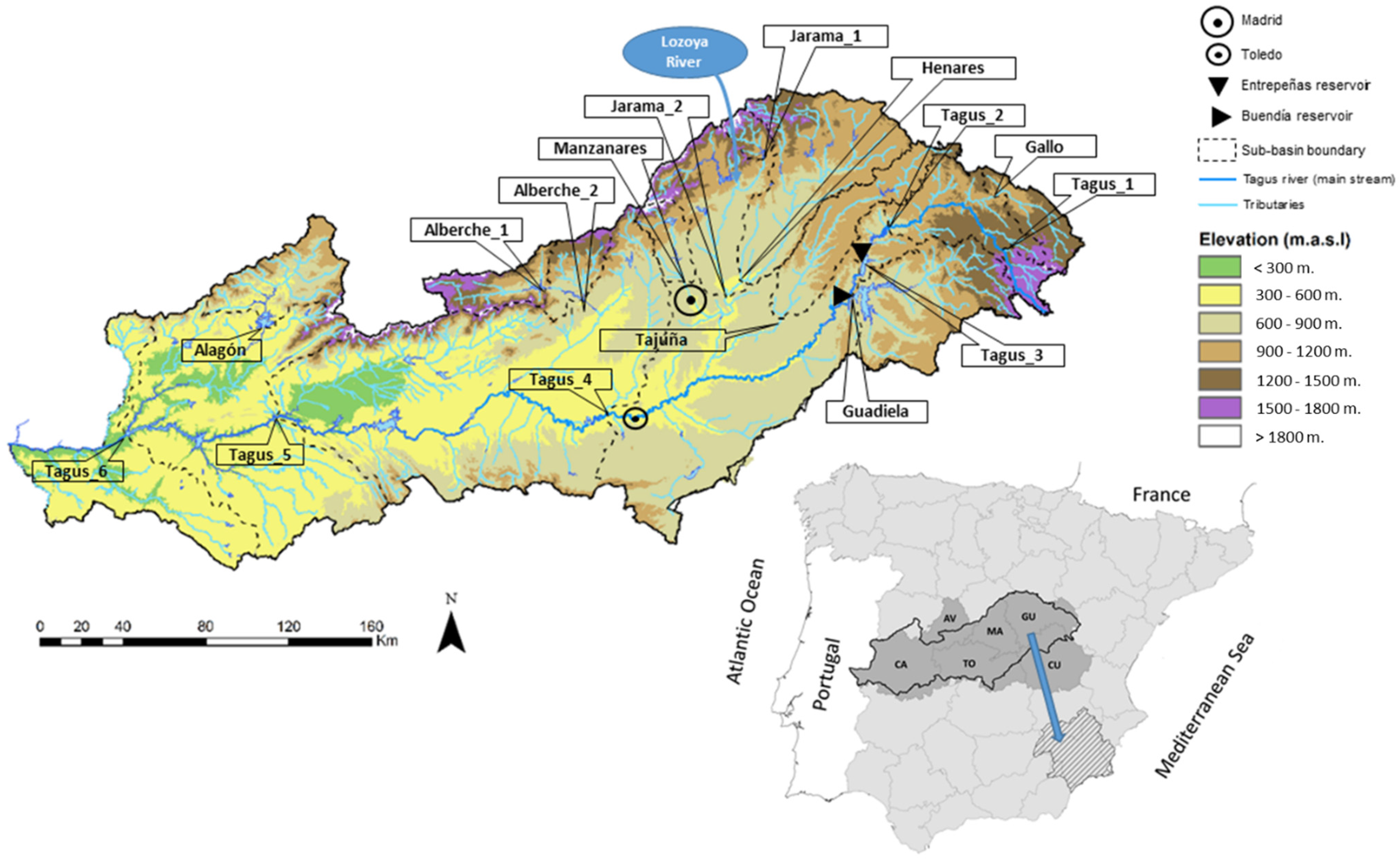
The Tagus River basin stretches over 81,447 km² across Spain (68%) and Portugal (32%) (Figure 1). Climate conditions follow a Mediterranean–continental pattern with two clearly different periods: a dry season during the summer and a wet season during winter and early spring. The altitude gradient along the east–west axis of the basin leads to marked differences in precipitation and temperature. The mean annual temperature ranges from 8 °C in the mountain peaks in the north to 17 °C in the west. The mean annual precipitation ranges from 1800 mm to less than 400 mm [30].

The Spanish part of the Tagus basin is home to more than 7.7 million people [24], which generates significant pressure on its water resources [31]. The upper part is the less populated part of the basin and is the source area of a major water transfer that diverts an average of 360 Hm³·year⁻¹ to the Mediterranean coast [32]. Water is diverted from the Entrepeñas and Buendía reservoirs, with a total storage capacity of 2518 Hm³ (23% of the total reservoir capacity in the basin). The urban areas of Madrid and Toledo are located in the middle part of the basin (see Figure 1) and host 5.1 and 0.6 million inhabitants, respectively. The water demand of the capital city—about 500 Hm³·year⁻¹—is met mainly from reservoirs in the Lozoya river [33] (see location in Figure 1) and is returned mostly to the Manzanares river, which is under pressure from the domestic pollution load [34,35].

Forested areas cover 25% of the basin and are located mainly in the highlands. Cropland, found mainly on the plains close to the Tagus River, is the second most significant land use in terms of surface area (32% of the basin). Urban areas and bare soil account for less than 2%, while grassland (including natural grassland, pasture and Mediterranean shrub vegetation) covers 39% of the territory, this being the predominant land cover in the basin.

Figure 1. Above: The spatial distribution of the studied sub-basins (see Table 1 for gauging station identification by river code). Below: Location of the Tagus basin in the Iberian Peninsula (black boundaries) and the main provinces in the basin (in dark grey: AV: Ávila; CA: Cáceres; CU: Cuenca; GU: Guadalajara; MA: Madrid; TO: Toledo). The blue arrow shows the Tagus–Segura water transfer.

Figure 1. Above: The spatial distribution of the studied sub-basins (see Table 1 for gauging station identification by river code). Below: Location of the Tagus basin in the Iberian Peninsula (black boundaries) and the main provinces in the basin (in dark grey: AV: Ávila; CA: Cáceres; CU: Cuenca; GU: Guadalajara; MA: Madrid; TO: Toledo). The blue arrow shows the Tagus–Segura water transfer.

Table 1. Main characteristics of the studied sub-basins. IR represents the accumulated impoundment ratio (i.e., regulatory capacity upstream divided by mean annual runoff).

River Code a	Code	Data Period	Drainage Area (Km2) b	Elevation (m.a.s.l) b	Mean Annual Runoff (Hm3) c	IR
Tagus_1	3001	1950–2010	410	1143	154	0.00
Tagus_2	3005	1950–2010	3253	720	556	0.00
Tagus_3	3006	1954–2010	3853	697	556	1.47
Tagus_4	3012	1965–2010	27,159	430	2026	1.93
Tagus_5	3017	1950–2010	41,610	186	5412	1.16
Tagus_6	3019	1950–2010	51,958	110	7231	1.50
Gallo	3030	1950–2010	944	1016	57	0.00
Guadiela	3043	1955–2010	3300	761	508	3.41
Jarama_1	3050	1950–2010	381	891	172	0.33
Jarama_2	3052	1950–2010	7005	550	777	1.30
Henares	3062	1950–2010	4031	565	347	0.88
Manzanares	3070	1950–2010	710	588	94	1.56
Tajuña	3082	1950–2010	2029	615	144	0.44
Alberche_1	3111	1950–2010	1045	719	403	0.51
Alberche_2	3112	1955–2010	1919	557	548	0.62
Alagón	3142	1955–2010	1814	329	885	1.03

^a Code number shown in Figure 1. ^b Drainage area and elevation referred to the gauging station [36]. ^c Mean annual runoff corresponding to the data period.

Table 1. Main characteristics of the studied sub-basins. IR represents the accumulated impoundment ratio (i.e., regulatory capacity upstream divided by mean annual runoff).

River Code a	Code	Data Period	Drainage Area (Km2) b	Elevation (m.a.s.l) b	Mean Annual Runoff (Hm3) c	IR
Tagus_1	3001	1950–2010	410	1143	154	0.00
Tagus_2	3005	1950–2010	3253	720	556	0.00
Tagus_3	3006	1954–2010	3853	697	556	1.47
Tagus_4	3012	1965–2010	27,159	430	2026	1.93
Tagus_5	3017	1950–2010	41,610	186	5412	1.16
Tagus_6	3019	1950–2010	51,958	110	7231	1.50
Gallo	3030	1950–2010	944	1016	57	0.00
Guadiela	3043	1955–2010	3300	761	508	3.41
Jarama_1	3050	1950–2010	381	891	172	0.33
Jarama_2	3052	1950–2010	7005	550	777	1.30
Henares	3062	1950–2010	4031	565	347	0.88
Manzanares	3070	1950–2010	710	588	94	1.56
Tajuña	3082	1950–2010	2029	615	144	0.44
Alberche_1	3111	1950–2010	1045	719	403	0.51
Alberche_2	3112	1955–2010	1919	557	548	0.62
Alagón	3142	1955–2010	1814	329	885	1.03

^a Code number shown in Figure 1. ^b Drainage area and elevation referred to the gauging station [36]. ^c Mean annual runoff corresponding to the data period.

2.2. Data Collection

2.2.1. Hydrological Data

We used discharge data from 16 gauging stations along 9 different rivers (Figure 1) that were selected from an original set of 187 stations using the following criteria: (a) they should have a record of at least 45 consecutive years of streamflow data in the period 1950–2010; and (b) missing data should account for less than 10% of the total data series. Streamflow data were obtained on a monthly scale and gaps were filled by linear regression (Pearson’s correlation threshold set to 0.8) using data from the same river or from nearby tributaries. Hydrological data were aggregated into the annual flow series (Hm³·year⁻¹) following the hydrological year (1 October–30 September). More than one station was retained in the Tagus River, as were two of its tributaries (Jarama and Alberche) (Table 1).

2.2.2. Climatic Data

Climatic data on a monthly scale were obtained from a countrywide database developed by González-Hidalgo et al. [10,11]. They carried out a process of reconstruction, deletion of incorrect data, gap filling, statistical analysis to detect inhomogeneity and interpolation to a 0.1° × 0.1° grid of historic records (1950–2010) of monthly precipitation (in mm) and average monthly temperature (in °C) from 2670 and 1358 weather stations, respectively. More information about the process followed to build the database can be found in [10,11]. For our study, we retrieved the complete (1950–2010) precipitation and temperature data series for the Tagus basin and aggregated them into annual values and by sub-basin.

2.2.3. Land Cover Data

We retrieved data on the evolution of land cover from the following sources:

• Historical dataset of land cover for Europe spanning from 1900 to 2010 developed by Fuchs et al. [37,38,39]. This database, available in raster maps of 1 km × 1 km resolution at a decadal scale, clusters land cover into six groups: forest, grassland, cropland, urban areas, water and other (including bare soil and sparsely vegetated areas).
• Data on the extension of irrigated land at a provincial level (the Tagus basin includes territories of 12 different provinces) from 1950 to 2010 with a 10-year temporal resolution, obtained from the National Institute of Statistics [40]. We considered only the provinces that cover more than 2% of the Tagus basin and that cumulatively represent over 97% of its territory (Ávila, Cáceres, Cuenca, Guadalajara, Madrid and Toledo).

2.3. Data Analysis

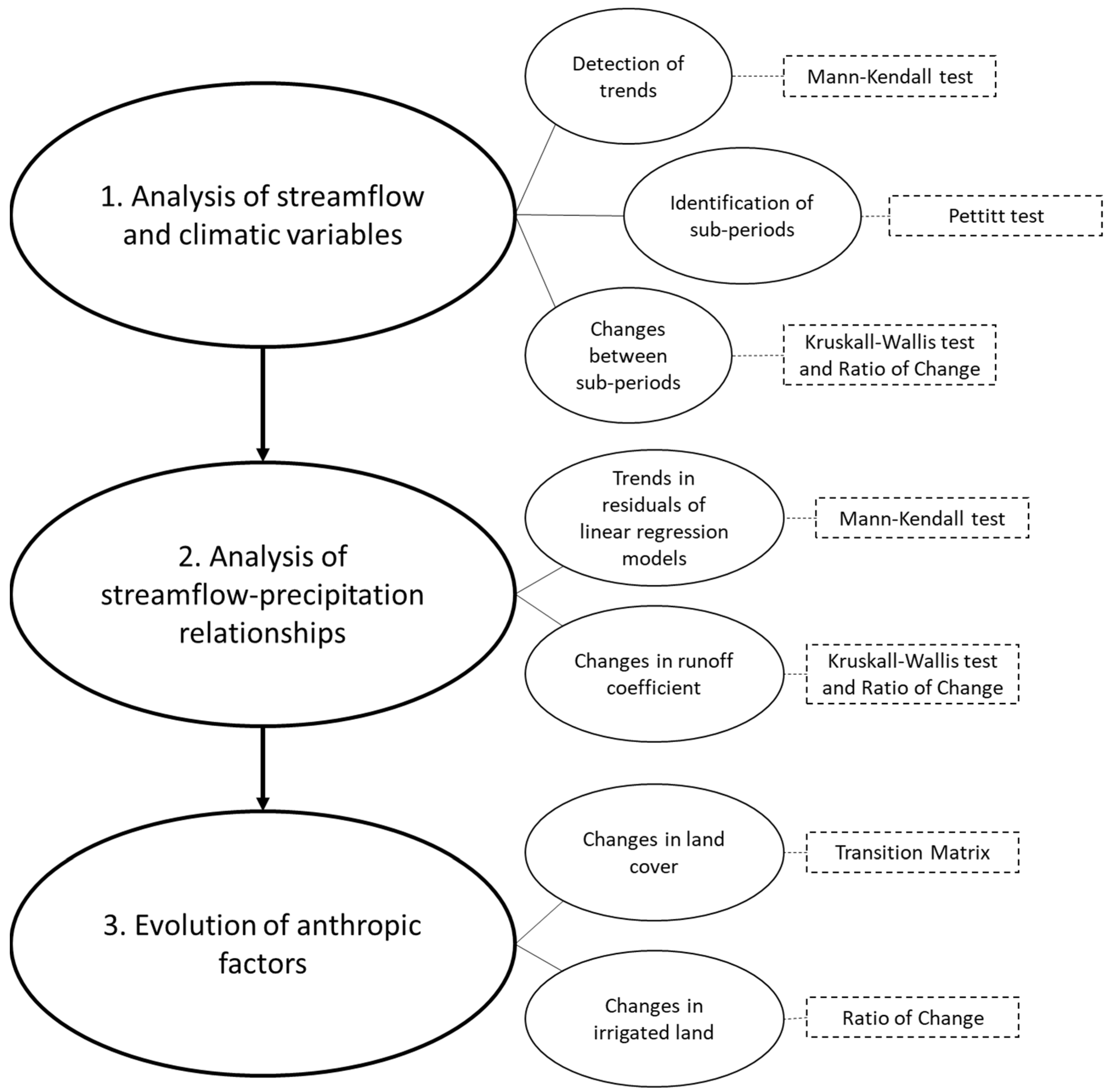
Figure 2 shows the steps followed in the study, specifying the type of analysis carried out and the methods used.

2.3.1. Analysis of Streamflow and Climatic Variables

Detection of Trends

In order to analyze trends in annual accumulated streamflow (Hm³ year⁻¹), mean annual precipitation (mm year⁻¹) and mean annual temperature (°C year⁻¹) in each of the selected sub-basins, we applied the non-parametric Mann–Kendall (MK) test [41,42], which has been widely used to assess the evolution of hydroclimatic series [6,10,11,13,43,44,45]. As a result of potential serial correlation in raw data series, we first applied the trend-free pre-whitening procedure described by Yue et al. [46]. Once the serial correlation was removed, the z-statistic obtained from the MK test was used to establish the sign, strength and significance of the trend. Positive and negative z-values indicate an increasing and decreasing trend, respectively. Following the criteria proposed by Gao et al. [43], $1.97<\left|Z\right|<2.57$ implies that the observed trend is significant (p-value < 0.05), while $\left|Z\right|>2.567$ indicates a highly significant trend (p-value < 0.01). Absolute z-values $\left|Z\right|<1.97$ indicate no significant trend (p-value > 0.05). The z-statistic was calculated using the R-package modifiedmk Version 1.5.0.

Identification of Sub-Periods

In order to analyze the existence of different sub-periods within the hydroclimatic time series, we used the Pettitt non-parametric test [47]. This test identifies significant break points and was used to assess the null hypothesis that when iteratively and randomly splitting the time data series into two time periods, there is no change in the mean value of each period. If p-value < 0.05, the null hypothesis can be rejected and therefore a significant break point be identified at t₀. Based on the results of the Pettitt test, the climatic and hydrological series were divided into sub-periods, using the year of t₀ as an inflection point.

In order to remove the effect of the Tagus–Segura water transfer in streamflow trends and break points in those river stretches affected by this transfer scheme (Tagus_4, Tagus_5 and Tagus_6), we added the total amount of water diverted each year [32] to the corresponding streamflow data series.

Changes between Sub-Periods

Changes between the sub-periods were quantified by applying the Kruskall–Wallis (KW) test. The null hypothesis of this non-parametric test evaluates whether the median value in each sub-period is similar. Then, we assessed the changes between the two sub-periods using the ratio of change (dV), which quantifies the deviation of the mean value of each variable after the break point:

$$d{V}_{pre-bp/post-bp}=\frac{X_{post-bp}-X_{pre-bp}}{X_{pre-bp}}\times 100 (\%)$$

(1)

where $X_{pre-a.ch}$ and $X_{post-a.ch}$ are the mean values of the pre- and post-break points.

2.3.2. Analysis of Streamflow–Precipitation Relationships

Trends in Residuals of Linear Regression Models

In order to explore the influence of precipitation on the evolution of streamflow, we developed a regression model for each sub-basin in which the annual precipitation was set as the explanatory variable and annual streamflow as the dependent variable. The mean annual temperature was not considered as an explanatory variable because previous work focused on the IP has been inconclusive as to whether the inclusion of temperature in regression models to explain streamflow evolution is significant (see [6,20,48]).

Input variables were normalized by subtracting the mean value of the period and dividing it by the standard deviation. Possible trends were removed prior to normalization to avoid their effect on the correlation between streamflow and precipitation. Once the models were adjusted, the trends in their residuals were explored using the MK test. The existence of these trends suggests that there are time-dependent variables different from precipitation that had an influence on streamflow evolution during the studied period [6,20,48].

Changes in Runoff Coefficients

We explored potential changes in the streamflow-precipitation relationship between sub-periods. For this purpose, we calculated the runoff coefficient (i.e., ratio between annual streamflow and precipitation) for each sub-period and ran the KW test to detect statistically significant differences.

2.3.3. Evolution of Anthropic Factors

Finally, we explored the temporal evolution of several anthropic factors that may have contributed to altering the relationships between precipitation and streamflow over time. These factors could partially explain the existence of trends in the residuals of the models and significant changes in runoff coefficients mainly referred to: (a) changes in land cover and, specifically, (b) changes in irrigated land. Land cover changes were detected by means of a landscape transition matrix detailed in the Appendix A (

Table A1. Transition matrix to classify land cover changes in the Tagus basin.

Land Uses Before	Land Uses After
	Forest	Grassland	Crop	Urban	Other land	Water
Forest
Grassland
Cropland
Urban
Other land
Water
	No change
	Forest expansion
	Forest degradation
	Cropland abandonment
	Conversion to agricultural land
	Pasture and shrubland expansion
	Urban and unproductive land expansion
	New water bodies

).

3. Results

3.1. Streamflow Analysis

3.1.1. Historical Trends, Break Points and the Influence of Regulation

All of the sub-basins exhibited negative trends in streamflow (z-value < 0 in all cases) (

Table 2. Results of the Mann–Kendall Test (expressed as z-values and mean increase/decrease) and the Pettitt test (expressed as year of change) for streamflow, precipitation and temperature in selected sub-basins of the Spanish part of the Tagus basin (1950–2010).

River Code	Mann-Kendall Test (z-Value)			Mean Increase/Decrease			Pettitt Test (Year)
	S	P	T	S (% Year−1)	P (mm Decade−1)	T (°C Decade−1)	S	P	T
Tagus_1	−1.15	−1.65	4.81 **	−0.55	−28.01	0.25	1988	1979	1981 *
Tagus_2	−2.81 **	−1.49	4.44 **	−1.15	−20.01	0.22	1980 *	1979	1984 *
Tagus_3	−5.00 **	−1.97 *	4.66 **	−1.34	−23.91	0.23	1980 *	1979 *	1985 *
Tagus_4	−5.16 **	−1.18	5.02 **	−3.01	−16.70	0.34	1981 *	1979	1984 *
Tagus_5	−2.60 **	−1.85	4.43 **	−1.04	−18.82	0.20	1979 *	1979 *	1984 *
Tagus_6	−3.21 **	−1.55	4.40 **	−1.41	−19.00	0.19	1979 *	1979	1984 *
Gallo	−3.53 **	−1.34	4.61 **	−1.06	−14.15	0.23	1980 *	1979	1981 *
Guadiela	−6.31 **	−2.71 **	4.60 **	−1.80	−34.97	0.22	1982 *	1980 *	1984 *
Jarama_1	−2.44 *	−2.31 *	4.52 **	−0.86	−21.90	0.19	1979 *	1980 *	1981 *
Jarama_2	−3.12 **	−1.79	4.35 **	−1.42	−15.42	0.19	1979 *	1979	1981 *
Henares	−0.45	−1.38	4.26 **	−0.44	−11.17	0.21	1958	1979	1981 *
Manzanares	−2.78 **	−2.31 *	4.52 **	−1.52	−23.04	0.20	1979 *	1979 *	1981 *
Tajuña	−6.08 **	−1.73	4.28 **	−3.54	−19.89	0.23	1979 *	1979	1984 *
Alberche_1	−2.65 **	−1.62	4.44 **	−0.76	−17.33	0.23	1979 *	1979	1984 *
Alberche_2	−2.61 **	−1.35	4.59 **	−1.19	−20.44	0.27	1979 *	1979	1984 *
Alagón	−2.18 *	−2.17 *	3.43 **	−1.07	−39.35	0.17	1970	1979	1986 *

Note: S: Streamflow; P: Precipitation; T: Temperature. * p-value < 0.05. ** p-value < 0.01.

) with a mean annual decrease for the entire basin of −1.38% (ranging from −0.44% to −3.54%). Decreases were statistically significant or highly significant in 2 and 12 gauging stations out of 16, respectively. Significant break points between 1979 and 1982 were detected in most of the cases (13 out of 16). Almost 85% of the significant break points were found in 1979 and 1980.

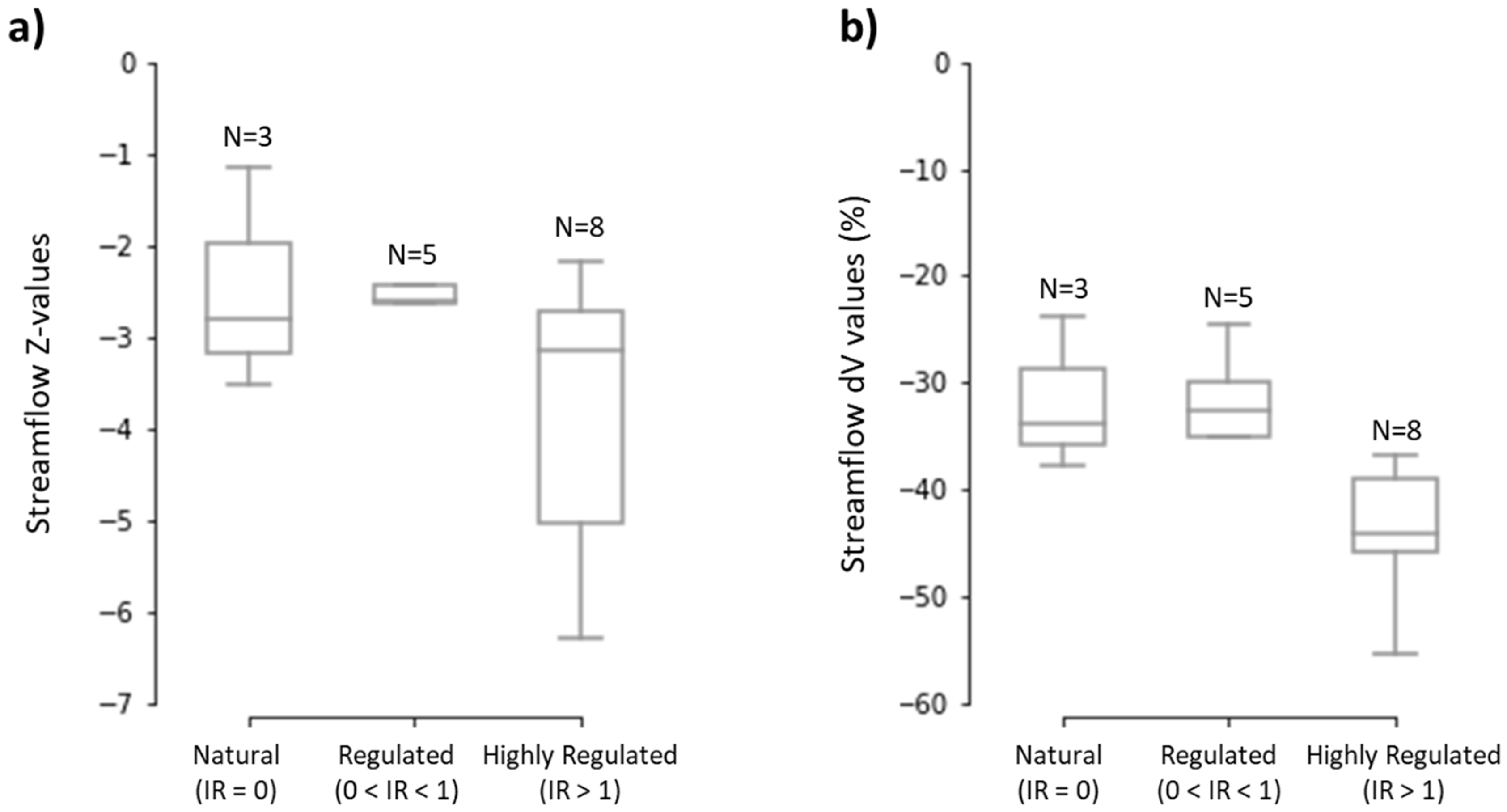
The strength of the negative trends observed in the streamflow did not show any geographic pattern in terms of altitude, location or drainage area. However, we found a relationship between the magnitude of trends (i.e., z-value) and the degree of impoundment of each sub-basin (Figure 3a), expressed as the ratio between upstream regulatory capacity and mean annual runoff (IR values in Table 1). Negative trends in free-flowing (IR = 0) and regulated (0 < IR <1) rivers were similar in magnitude and range of variability, whereas the decline in streamflow was sharper and more variable in highly regulated rivers (IR > 1). These results suggest that river damming exacerbated the observed hydrological decline in terms of magnitude and variability.

3.1.2. Magnitude of Changes in Streamflow between Sub-Periods

Based on the most frequent dates of the break points, we selected the year 1979–1980 as the limit between two distinct sub-periods (1950–1979 and 1980–2010).

Table 3. Magnitude (dV) and significance of changes in streamflow, precipitation, temperature and runoff coefficient between 1950–1979 and 1980–2010. Asterisks indicate that changes in the median values of each sub-period were statistically significant. Note: S: Streamflow; P: Precipitation; T: Temperature; RC: Runoff coefficient.

River Code	S dV (%)	P dV (%)	T dV (%)	RC dV (%)
Tagus_1	−23.7 *	−15.6 **	9.8 **	−10.1
Tagus_2	−37.9 **	−14.0 **	7.9 **	−27.3 **
Tagus_3	−39.6 **	−15.0 **	7.4 **	−29.4 **
Tagus_4	−55.5 **	−14.3 *	7.7 **	−48.0 **
Tagus_5	−36.9 **	−14.1 **	5.8 **	−28.6 **
Tagus_6	−45.1 **	−13.6 *	6.1 **	−38.8 **
Gallo	−33.8 **	−12.5 *	8.4 **	−25.4 **
Guadiela	−43.2 **	−18.3 **	6.4 **	−29.1 **
Jarama_1	−30.0 **	−14.7 **	6.8 **	−19.9 **
Jarama_2	−47.4 **	−12.7 **	6.2 **	−41.5 **
Henares	−32.6	−11.0 *	6.0 **	−23.0
Manzanares	−45.5 **	−14.9 **	6.5 **	−41.9 **
Tajuña	−70.1 **	−14.2 **	6.5 **	−65.3 **
Alberche_1	−24.6 **	−11.0 *	7.2 **	−20.1 **
Alberche_2	−35.1 **	−11.3 *	7.4 **	−30.4 **
Alagón	−26.3 *	−15.7 *	4.6 **	−10.6
Mean	−39.2	−13.9	6.9	−30.6
Maximum	−70.1	−18.3	9.8	−65.3
Minimum	−23.7	−11.0	4.6	−10.1

* p-value < 0.05; ** p-value < 0.01.

details the magnitude of changes between periods using the ratio of change (dV) and the significant differences as determined by the KW test.

Most sub-basins (15 out of 16) experienced significant changes in streamflow between sub-periods, with a −39% mean reduction across the considered gauging sites. No clear spatial patterns could be identified, but a similar trend was found when comparing the degree of impoundment with the magnitude of streamflow reductions between periods (Figure 3b). For free-flowing and regulated rivers (IR = 0 and 0 < IR < 1 respectively), the annual streamflow during the first sub-period was around 30% lower than in the second one. This percentage exceeds the 40% reduction in highly regulated rivers (IR > 1), which confirms that when regulation capacity exceeds the mean annual runoff, streamflow decline is exacerbated.

3.2. Analysis of Climatic Variables: Precipitation and Temperature

3.2.1. Historical Trends and Break Points

Precipitation presented a generalized negative trend over time (Table 2) but decreasing trends (a mean decrease of −22 mm per decade) were significant or highly significant in only five sub-basins. These include the two sub-basins draining to the reservoirs that supply the Tagus–Segura water transfer (i.e., Tagus_3 and Guadiela) and the Jarama_1, Manzanares and Alagón rivers. All the break points emerged in 1979 or 1980 but, in contrast to streamflow results, they were significant (p-value < 0.05) in only 5 out of 16 cases.

The application of the MK test (Table 2) to temperature data revealed highly significant increasing trends in all the sub-basins, with the z-statistic values ranging between 4 and 5 for almost all the stations. Average annual increase was 0.22 °C per decade and the magnitude of temperature trends was quite uniform across the basin, as shown by the relatively narrow range of z-values. According to the Pettitt test, all the data series exhibited significant break points between 1981 and 1986.

3.2.2. Magnitude of Changes in Climatic Variables between Sub-Periods

All the sub-basins experienced significant reductions in precipitation between sub-periods, with a mean reduction of −14% (Table 3), ranging from −11% to −18%. Temperature on average increased by 7%, with variations ranging between 5% and 10%. No spatial pattern could be detected in the case of precipitation, but we found a positive correlation between changes in temperature and the altitude of each gauging station (Pearson’s r = 0.78; p-value < 0.05). Although the increase in mean annual temperature occurred throughout the basin, altitudes above 500 m.a.s.l. and especially those above 1000 m.a.s.l. experienced larger increases.

3.3. Analysis of Streamflow–Precipitation Relationships

3.3.1. Trends in Residuals of Linear Regression Models

The results presented in the previous sections indicate that the evolution of streamflow did not follow the same pattern as was observed for precipitation. Thus, we explored the extent to which this divergence could be related to other factors.

Table 4. Coefficients of regression for predicting streamflow (S) from precipitation (P). R² indicates the efficiency of each model. Z_residuals represent the sign and strength of trends in the residuals of the models. The intercept was omitted since it was not significant in the models. In the first column, asterisks indicate whether the variable was significant in the models. In the last column, they indicate whether the trends in residuals were significant.

River Code	Dependent Variable: S (Streamflow)
	P	R2	Zresiduals
Tagus_1	0.772 ***	0.60	−0.44
Tagus_2	0.839 ***	0.70	−2.87 ***
Tagus_3	0.419 **	0.18	−4.16 ***
Tagus_4	0.589 ***	0.35	−4.11 ***
Tagus_5	0.876 ***	0.78	−2.02 ***
Tagus_6	0.879 ***	0.77	−2.96 ***
Gallo	0.65 ***	0.42	−3.43 ***
Guadiela	0.241 *	0.06	−5.43 ***
Jarama_1	0.833 ***	0.69	−2.35 ***
Jarama_2	0.74 ***	0.55	−2.52 ***
Henares	0.618 ***	0.38	−0.15
Manzanares	0.755 ***	0.57	−0.27
Tajuña	0.576 ***	0.33	−5.37 ***
Alberche_1	0.739 ***	0.55	−2.00 ***
Alberche_2	0.826 ***	0.69	−2.07 ***
Alagón	0.796 ***	0.63	0.30

* p-value < 0.1; ** p-value < 0.05; *** p-value < 0.01.

shows the results of linear regression models built to predict annual streamflow from precipitation in each sub-basin. R² ranged between 0.06 and 0.78, pointing to an uneven influence of precipitation on the evolution of the streamflow across sub-basins. In general, gauging stations with larger percentages of explained variance are located mostly in non-regulated rivers or where accumulated storage capacity is close to 1 or lower. In these sub-basins, the annual pattern of flow regime mimics the annual precipitation regime better. Gauging stations that displayed the lowest percentages of explained variance in the models (R² < 0.20) are located immediately downstream of the reservoirs of the Tagus–Segura water transfer (Tagus_3 and Guadiela). In those stations, upstream storage capacity exceeds by far the mean annual streamflow, which seems to be the main factor in explaining the low correlation between precipitation and streamflow. We detected a significant negative correlation between IR and the R² (Pearson’s r = −0.52; p-value < 0.05), suggesting that the efficiency of the models was related to the level of impoundment of each sub-basin.

This is even more evident in the Tagus River. The lowest percentages of R² are found for the gauging sites along the medium stretches of the river (i.e., Tagus_3 and Tagus_4, with IR values of 1.47 and 1.93, respectively), while linear models exhibited higher efficiency for the other gauging sites (e.g., Tagus_2 and Tagus_5, with IR values of 0 and 1.16, respectively). Possibly, the absence of large water withdrawals in the upper parts of the basin and returns from water uses in lower parts contribute to an explanation of this finding.

The residuals of the models exhibited a significant negative trend over time in 12 out of 16 sub-basins. Downward trends were observed for both regulated and non-regulated rivers with no clear spatial pattern. This circumstance indicates that the evolution of time-dependent variables different from precipitation has influenced the observed decline in streamflow trends during the period studied.

3.3.2. Changes in the Runoff Coefficient

As expected from previous results, the runoff coefficient decreased between sub-periods in all of the sub-basins, and differences were statistically significant in most of the cases (13 out of 16) (Table 3). The mean reduction was −31%, ranging from −10% to −65%. Runoff reductions correlated significantly with the strength of the negative trends in the residuals of the model (Pearson’s r = 0.58; p-value < 0.05), suggesting that the temporal evolution of non-rainfall-related factors have altered the relationship between streamflow and precipitation. These changes meant that the capacity of rainfall to generate runoff significantly decreased in the Tagus basin after 1980.

3.4. Evolution of Anthropic Factors

3.4.1. Changes in Land Cover

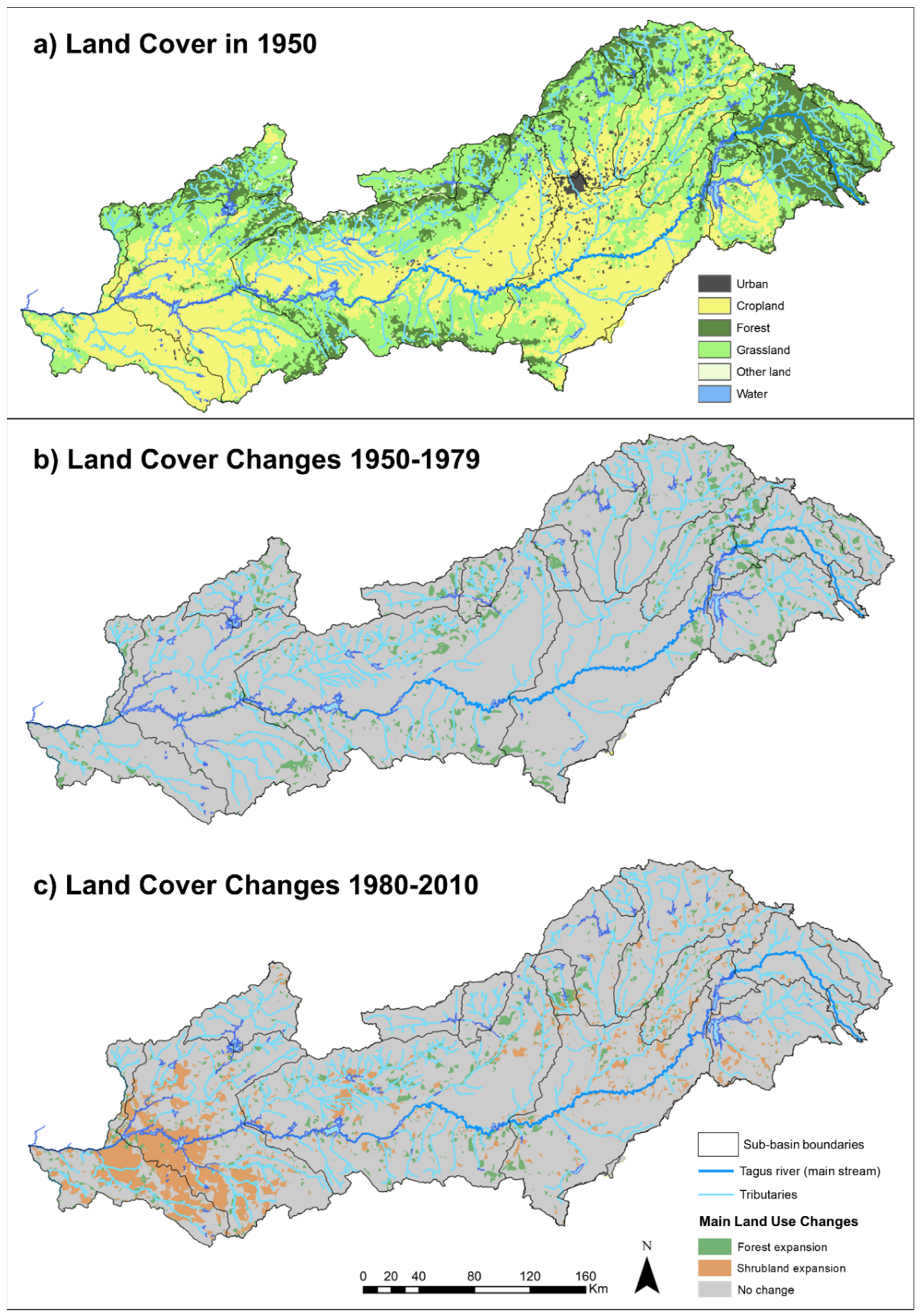
We analyzed land cover changes in the Tagus basin between the sub-periods 1950–1979 and 1980–2010 (Figure 4; see numerical values in

Table A2. Transition matrix of land cover changes between 1950–1980.

Land Cover 1950	Land Cover 1980						Total 1950
	Forest	Grassland	Cropland	Urban	Other Land	Water
Forest	7733	626	85	29	9	1	8483
Grassland	3802	16,256	1853	78	7	19	22,015
Cropland	324	688	22,297	282	1	17	23,609
Urban	5	9	34	612	0	0	660
Other land	11	12	1	0	388	0	412
Water	8	4	7	0	0	471	490
Total 1980	11,883	17,595	24,277	1001	404	509	55,669
47,757	No change
4150	Forest expansion
626	Forest degradation
688	Cropland abandonment
1980	Conversion to agricultural land
25	Pasture and shrubland expansion
406	Urban and unproductive land expansion
37	New water bodies

and

Table A3. Transition matrix of land cover changes between 1980–2010.

Land Cover 1980	Land Cover 2010						Total 1980
	Forest	Grassland	Cropland	Urban	Other Land	Water
Forest	11,210	631	24	12	4	2	11,883
Grassland	2013	15,304	222	44	5	7	17,595
Cropland	394	5764	17,984	115	2	18	24,277
Urban	5	16	21	959	0	0	1001
Other land	2	6	1	0	395	0	404
Water	4	7	5	0	0	493	509
Total 2010	13,628	21,728	18,257	1130	406	520	55,669
46,345	No change
2418	Forest expansion
631	Forest degradation
5764	Cropland abandonment
273	Conversion to agricultural land
29	Pasture and shrubland expansion
182	Urband and unproductive land expansion
27	New water bodies

).

In the 1950s, approximately 80% of the basin was covered by pastures, Mediterranean shrub and crops. Only 16% of the surface was occupied by forests, mostly located in the headwaters. Urban use represented only 1.5% of the area (Figure 4a). Three decades later, in 1980, the land cover had experienced marked changes (Figure 4b). The surface of arable land had remained nearly constant, while the forested area had registered a relative increase of +40%. This expansion was especially evident in the headwaters of the Tagus River and the highlands of the north and northwest of the basin. In absolute terms, the forested area gained 3400 km² between 1950 and 1979. This growth was mainly due to the replacement of natural pastures, which were reduced by −20% (−4420 km²). In parallel, during this period there was a significant increase in urban areas (+52% or +341 km² in absolute values), especially due to the growth of the city of Madrid.

Between 1980 and 2010 (Figure 4c), the most remarkable change in land cover was the decrease of cropland (−25% or −6020 km²), accompanied by an increase in both forest and Mediterranean shrubland (+15% and +23%, respectively; 5878 km² in total). During this period, forest expansion was more intense in areas at medium or high altitudes in the north and south of the basin whereas the expansion of Mediterranean shrub and pastures was more intense in the lower lands, located in the western part of the basin.

Considering changes during the whole period studied (i.e., from 1950 to 2010), our results reveal that the main land cover changes in the basin consisted of marked forest expansion (relative growth of 60%, which represents an increase of +5145 km²) at the expense, mainly, of cropland areas (relative decrease of −23%, −5352 km²).

3.4.2. Evolution of the Irrigated Area

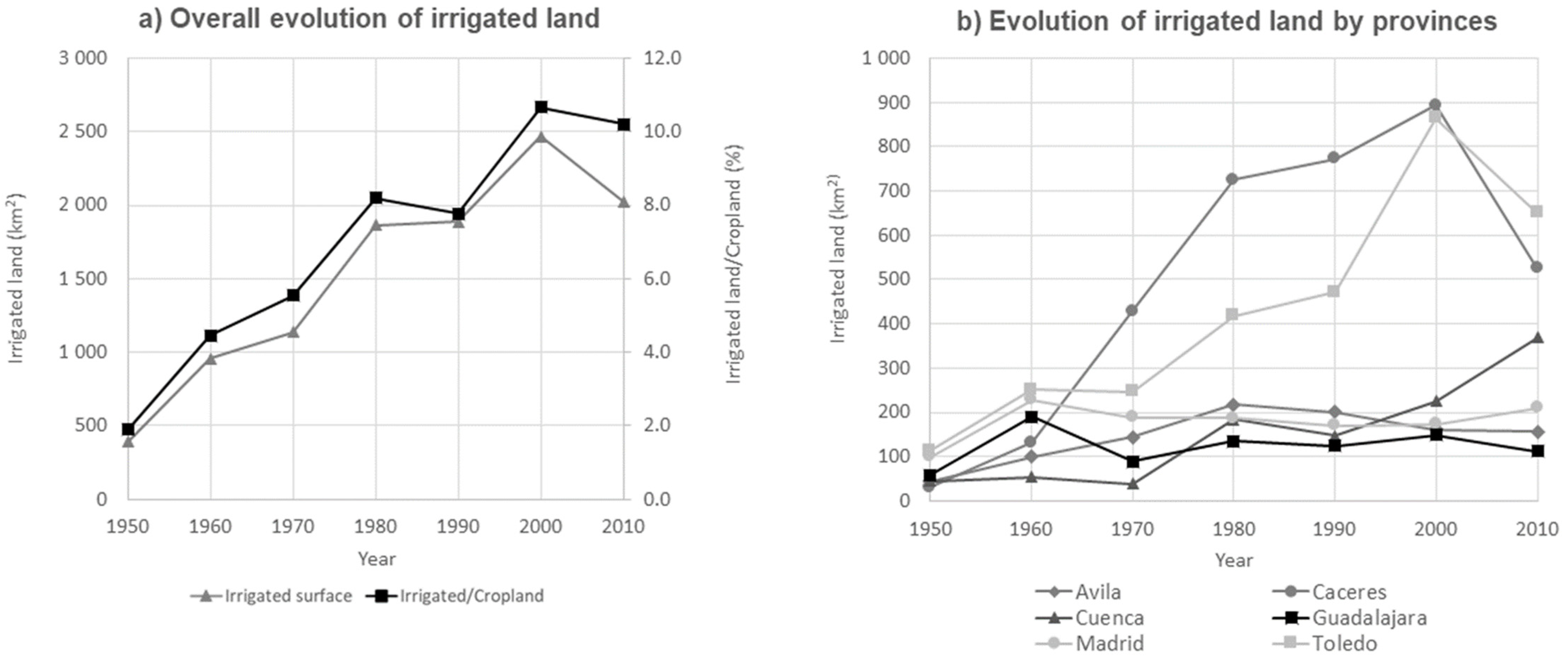
The irrigated area experienced an increase from less than 400 km² in 1950 to almost 2000 km² in 2010 (+400%) (Figure 5a). The ratio between irrigated land and cropland increased from less than 2% in 1950 to more than 10% in the year 2010. The relative growth in irrigated land was more intense from 1950 to 1980 (+376%) than from 1980 to 2010 (+8%).

The expansion of irrigated land in the last 60 years has been uneven across the Tagus provinces (Figure 5b). In the provinces located in the central and eastern part of the basin (Cuenca, Guadalajara, Madrid and Ávila) the growth was moderate throughout the period studied, while in the central and western part of the basin (Toledo and Cáceres) the surface of irrigated land experienced a sharp increase, especially from 1970 to 2000.

4. Discussion

4.1. Streamflow Changes vs. Changes in Climatic Variables

The evolution of streamflow followed a generalized downward trend in most of the sub-basins, with a significant break point around 1980. The observed mean streamflow decline (annual decrease of −1.38%) was similar to those reported in other basins in central Spain (i.e., Guadiana and Guadalquivir, between −1% and −3% for the period 1945–2005), but it was slightly higher than for the rest of the IP (below 1% per year) [13]. A decrease in annual streamflow around 1980 has also been reported in other Southern European rivers in Rumania, Bulgaria, Slovenia, Croatia and Turkey [49,50,51,52].

In contrast, precipitation trends were not significant in most of the cases. This is in line with findings by De Castro et al. [53], who studied the evolution of rainfall in Spain and concluded that the identification of trends on a large scale is complex due to high temporal, seasonal and spatial variability. Indeed, the study of the longest rainfall series (more than a century) [54,55] and data series similar to those used in the present study did not detect clear trends in annual precipitation in central Spain [10].

The z-statistics were negative in all the sub-basins studied and the mean reduction of precipitation was −22 mm per decade (Table 2). This result is consistent with generalized reductions detected in the Mediterranean region for similar time periods. However, reductions in the Tagus basin were slightly less pronounced than those reported by Philandras et al. [3] for western Europe (−36 mm per decade in the period 1951–2010) or those reported by the European Environmental Agency [2] for the IP (ranging from 0 to −60 mm per decade over the 1961–2006 period).

Interesting trends were identified in some of the sub-basins studied. Precipitation in the sub-basins draining into the reservoirs that feed the Tagus–Segura water transfer exhibited significant downward trends (Tagus_3 and Guadiela; see Table 2). This was also found by Lorenzo-Lacruz et al. [56] using data from 1961–2006 obtained from nine weather stations. Despite the observed negative trends in precipitation, the volume of water diverted by the Tagus–Segura transfer has followed an increasing trend since its inauguration in 1979 [26].

The generalized increasing trend of annual temperature that has accelerated since the 1980s could largely explain the divergence between precipitation and streamflow patterns. The observed rate of increase in temperature was homogeneous across the basin, reaching 0.22 °C per decade, slightly less pronounced than that observed in nine weather stations in southern Spain for the period 1960–2005 (0.28 °C per decade [57]) but higher than increases reported globally (0.20 °C per decade since 1975 [58]).

Although increasing temperature was recorded throughout the basin, we found a positive correlation between the magnitude of change (dV values) and the elevation of the sub-basin. One of the reasons that could explain this finding lies in the snow/ice–albedo relationship [59,60], as the reduction in snow cover duration decreases local albedo, which in turn leads to an increased absorption of solar radiation.

It is widely acknowledged that global warming affects the availability of water resources [61]. Increasing temperatures, combined with changes in other parameters, such as wind speed or humidity, affect evapotranspiration rates and the proportion of precipitation that turns into surface runoff and groundwater flow [62]. Therefore, the trends in temperature observed in this study are likely to have influenced the relationship between precipitation and surface runoff.

The analysis of the residuals left by the regression models (with highly significant downward trends in 12 out of 16 cases; see Table 4) confirms the existence of time-dependent variables influencing the streamflow decline in most areas of the Tagus basin. Our results reinforce similar findings in other parts of Spain. In the Ebro basin, López-Moreno et al. [44] found that 70 out of 88 sub-basins (i.e., 80%) displayed strong (p-value < 0.05) or moderate (p-value < 0.10) negative trends in residuals for the period 1950–2006 using linear regression models. With the same type of models, Vicente-Serrano et al. [6] found that 78% of 1204 gauging stations analyzed in Spain exhibited a negative residual trend, significant in 35%.

4.2. Streamflow Changes vs. Anthropic Factors

4.2.1. Degree of Flow Regulation

Our study suggests that high degrees of regulation exacerbated both the magnitude of trends and the reductions in streamflow observed between sub-periods (Figure 3). Whereas rivers with IR < 1 exhibited similar z-statistic and dV values, a difference occurs when the accumulated reservoir capacity exceeds the mean annual runoff (i.e., IR > 1). This finding is consistent with previous studies, in which direct links between the reduction in streamflow and the degree of flow regulation were found in several rivers in the northeast of the IP [63,64]. The large amount of resources derived to meet water demands in highly regulated basins and the larger areas exposed to the effects of temperature after dam construction could explain this finding.

Other circumstances, such as intense groundwater exploitation, could have played an important role in the reduction in streamflow [1]. As an illustrative example in Spain, the intensive use of groundwater in the Mancha Oriental aquifer since the 1980s has greatly contributed to the reduction in annual streamflow in the Júcar river [20].

4.2.2. Forest Expansion

As explained earlier, land cover changes between the periods 1950–1979 and 1980–2010 were mainly the result of an increase in forested areas at the expenses of cropland. In the period 1950–1980, forest expansion occurred in parallel with the loss of pasture and Mediterranean shrubland. This trend could be related to national policies promoted by the Spanish government at the end of the 1940s and in the 1950s. In 1939, the National Reforestation Plan foresaw the afforestation of 60,000 km² of non-agricultural lands (mainly with coniferous species) over a period of 100 years [65]. In the Tagus basin, this plan meant the afforestation of 3000 km², which is very similar to the expansion in forested area observed in the present study between 1950 and 1980 (3400 km²).

The observed expansion of both forest and shrubland in the Tagus basin (5878 km² between 1980 and 2010) occurred in parallel with cropland reduction (−6020 km²). This trend is compatible with the progressive farmland abandonment due to migration from rural to urban areas that occurred throughout the whole of the 20th century in many Mediterranean regions. This demographic shift is considered to be a driver of forest expansion in Spain between 1970 and 2000 [66].

The expansion of forests has important hydrological implications that mainly depend on the size of the basin, the type of forest and predominant climatic conditions [67]. However, it is widely acknowledged that afforestation processes increase evapotranspiration [68] and rainfall interception rates [69] and affect soil moisture [70], thus modifying precipitation–runoff dynamics [64]. The mean evapotranspiration associated with coniferous forest is around 1.3 and 1.4 times higher than the mean evapotranspiration values for rainfed traditional cropland and Mediterranean pasture–shrubland calculated for a region of central Spain [71]. Accordingly, several authors have suggested that runoff changes in high altitude non-regulated basins can only be explained by the modification of evapotranspiration rates produced by changes in land cover [20,44,48]. In our study, two high altitude, non-regulated sub-basins that experienced an expansion of their forested areas (i.e., Tagus_2 and Gallo) exhibited significant trends in model residuals and changes in runoff coefficients in the periods 1950–1979 and 1980–2010. Afforestation can explain these changes in the first study period while in the second one they could be the result of the combination of forest expansion and the significant acceleration in temperature increase that began in the early 80s.

In sub-basins located at lower altitudes, streamflow decline and changes in runoff coefficients cannot be explained solely by the combination of changes in climatic factors and land cover. In these cases, water withdrawals to meet irrigation and domestic demands may have played an important role in the modification of the precipitation–streamflow relationships.

4.2.3. The Development of Irrigated Agriculture and Other Local Factors

In parallel with farmland abandonment, traditional rainfed crops were gradually substituted by irrigated crops, the area of cultivation increasing from less than 400 km² in 1950 to almost 2000 km² in 2010, especially in the central and western parts of the Tagus basin. In relative terms, this growth in the Tagus basin was almost four times larger than that experienced in the whole country from 1950 to 1996 (a relative increase of 127%) [72].

Irrigated agriculture may affect water availability in rivers through two mechanisms. First, as a result of water withdrawals from surface and groundwater bodies. Using the average theoretical net water demand for irrigated crops as stated in the National Irrigation Plan for the Tagus basin (4905 m³·ha⁻¹ year⁻¹) [73], the expansion of irrigated areas led to an increase in water demand from 196 Hm³ ·year⁻¹ to 1177 Hm³·year⁻¹ between 1950 and 2010. This increase was accompanied by an unprecedented growth in the number of reservoirs in Spain [72], and the Tagus basin became the largest basin in Spain in terms of storage capacity [74].

The second mechanism is related to the evapotranspiration rates of irrigated land compared to other land uses. For instance, evapotranspiration rates in irrigated crops are 2.2 and 2.0 times higher than those of pasture–shrubland and rainfed annual crops, respectively [71]. Therefore, the growth of irrigated land combined with the increase in temperature in the basin is very likely to have contributed to the observed changes in the runoff coefficient. Vicente-Serrano et al. [6] suggested that the expansion of the irrigation surface in southwest Europe since the 1960s and the increase in atmospheric evaporative demand are among the main drivers explaining the reduction in streamflow in this region.

Finally, it is important to note that other water uses may explain specific observed trends. For instance, the Jarama_2 gauging station is located downstream from the main reservoirs that supply water to the city of Madrid, whose treated wastewater is returned into a different river. Therefore, the evolution of water diverted for domestic supply has played a major role in streamflow evolution in this sub-basin. Demographic evolution in the metropolitan area of Madrid (from 1.82 Mhab in 1950 to 6.57 Mhab in 2010; [75]) implies that urban water supply in this region has increased from about 100 Hm³·year⁻¹ in 1950 to more than 500 Hm³·year⁻¹ in 2010 [33].

4.2.4. Hydrological Decline Implications for Sustainable Water Management

Future scenarios of climate change have foreseen a generalized decrease in water availability in the region ranging from −4.2% to −11.0% for the period 2010–2040 and from −13.0% to −19.0% until 2070, depending on the greenhouse emission scenario considered (RCP 4.5 and 8.5, respectively) [12]. Therefore, if current water demands remain unchanged, water stress in the basin is likely to increase in the coming decades. This circumstance will complicate the operations of the Tagus–Segura water transfer, exacerbating existing tensions between water users in both basins. Moreover, the Tagus River Basin Authority will need to manage this likely decrease in water availability carefully in order to meet the water delivery obligations to Portugal and avoid additional degradation of river ecosystems.

Under this complex scenario, the implementation of e-flows is considered as one of the main actions that should be taken to maintain and improve the river’s resilience to climate change [76]. Since the pre-existing uses of water greatly affect the capability of River Basin Authorities to implement e-flows [77], an improvement in the river ecosystem will require revisiting and renegotiating current water allocation in the light of climate change and the pressing need to reverse the degradation of aquatic ecosystems.

5. Conclusions

The present study has found a generalized decrease in annual streamflow in the Tagus River basin since 1950 that cannot be explained solely by changes in precipitation patterns. This has been observed in terms of magnitude of trends, break points and magnitude of changes between the two periods established before and after 1980 (i.e., 1950–1979 and 1980–2010). The increase in temperature and the expansion of forest and irrigated land were identified as significant drivers of the observed hydrological changes in the basin. Other factors, such as water diversion to supply domestic needs, may have played an important role at a local level. Thus, the decline in streamflow in the Tagus basin can be linked to management decisions related to different sector policies, such as forest management, irrigation development and urban planning. Under future scenarios of increasing water scarcity and high competition for water resources, water management strategies should be based on effective inter-sector and inter-administrative cooperation seeking the resilience of the water system as a whole.

References

- García-Ruiz, J.M.; López-Moreno, I.I.; Vicente-Serrano, S.M.; Lasanta-Martínez, T.; Beguería, S. Mediterranean water resources in a global change scenario. Earth-Sci. Rev. 2011, 105, 121–139. [Google Scholar] [CrossRef] [Green Version]
- European Environment Agency (EEA). Water Resources across Europe—Confronting Water Scarcity and Drought; Publications Office of the European Union: Luxemburg, 2009; pp. 1–90. [Google Scholar]
- Philandras, C.M.; Nastos, P.T.; Kapsomenakis, J.; Douvis, K.C.; Tselioudis, G.; Zerefos, C.S. Long term precipitation trends and variability within the Mediterranean region. Nat. Hazards Earth Syst. Sci. 2011, 11, 3235–3250. [Google Scholar] [CrossRef] [Green Version]
- Alpert, P.; Krichak, S.O.; Sha, H.; Haim, D.; Osetinsky, I. Climatic trends to extremes employing regional modeling and statistical interpretation over the E. Mediterranean. Glob. Planet. Change 2008, 63, 163–170. [Google Scholar] [CrossRef]
- Camuffo, D.; Bertolin, M.; Barriendos, C.; Dominguez-Castro, F.; Cocheo, C.; Enzi, S.; Sghedoni, M.; della Valle, A.; Garnier, E.; Alcoforado, M.; et al. 500-year temperature reconstruction in the Mediterranean Basin by means of documentary data and instrumental observations. Clim. Change 2010, 101, 169–199. [Google Scholar] [CrossRef]
- Vicente-Serrano, S.M.; Peña-Gallardo, M.; Hannaford, J.; Murphy, C.; Lorenzo-Lacruz, J.; Dominguez-Castro, F.; Lopez-Moreno, J.I.; Beguería, S.; Noguera, B.I.; Harrigan, S.; et al. Climate, Irrigation and Land Cover Change Explain Streamflow Trends in Countries Bordering the Northeast Atlantic. Geophys. Res. Lett. 2019, 46, 10821–10833. [Google Scholar] [CrossRef] [Green Version]
- European Environment Agency (EEA). Use of Freshwater Resources—Indicator Assessment; Publications Office of the European Union: Luxemburg, 2018; Volume 63, pp. 74–85. [Google Scholar]
- European Commission (EC). Water Scarcity and Drought in the European Union; Publications Office of the European Union: Luxemburg, 2010; pp. 1–4. [Google Scholar]
- European Environment Agency (EEA). Water Use in Europe—Quantity and Quality Face Big Challenges; Publications Office of the European Union: Luxemburg, 2018; pp. 1–8. [Google Scholar]
- González-Hidalgo, J.C.; Brunetti, M.; De Luis, M. A new tool for monthly precipitation analysis in Spain: MOPREDAS database (monthly precipitation trends December 1945–November 2005). Int. J. Climatol. 2011, 31, 715–731. [Google Scholar] [CrossRef]
- González-Hidalgo, J.C.; Peña-Angulo, D.; Cortesi, N. MOTEDAS: A new monthly temperature database for mainland Spain and the trend in temperature (1951–2010). Int. J. Climatol. 2015, 35, 4444–4463. [Google Scholar] [CrossRef]
- CEDEX. Evaluación del Impacto del Cambio Climático en los Recursos Hídricos y Sequías en España; Ministerio de Agricultura, Pesca y Medio Ambiente: Madrid, Spain, 2017; pp. 1–346. [Google Scholar]
- Lorenzo-Lacruz, J.; Vicente-Serrano, S.M.; López-Moreno, J.I.; Morán-Tejeda, E.; Zabalza, J. Recent trends in Iberian streamflows (1945–2005). J. Hydrol. 2012, 414, 463–475. [Google Scholar] [CrossRef]
- Martínez-Fernández, J.; Sánchez, N.; Herrero-Jiménez, C. Recent trends in rivers with near-natural flow regime: The case of the river headwaters in Spain. Prog. Phys. Geogr. 2013, 37, 685–700. [Google Scholar] [CrossRef]
- Cazcarro, I.; Duarte, R.; Sánchez-Chóliz, J. Economic growth and the evolution of water consumption in Spain: A structural decomposition analysis. Ecol. Econ. 2013, 96, 51–61. [Google Scholar] [CrossRef]
- EEA. European Environment Agency. Waterbase-Water Quantity. Available online: https://www.eea.europa.eu/data-and-maps/data/waterbase-water-quantity-13 (accessed on 14 April 2021).
- Ministerio para la Transición Ecológica (MITECO). Síntesis de los Planes Hidrológicos Españoles. Segundo Ciclo de la Directiva Marco del Agua (2015–2021); MITECO: Madrid, Spain, 2018.
- Sánchez Pérez, M.A. Informe Hidrológico sobre la Gestión del Macro Embalse de Entrepeñas y Buendía; Universidad de Castilla la Mancha: Ciudad Real, Spain, 2018. [Google Scholar]
- Bromley, J.; Cruces, J.; Acreman, M.; Martínez, L.; Llamas, M. Problems of Sustainable Groundwater Management in an Area of Over-exploitation: The Upper Guadiana Catchment, Central Spain. Int. J. Water Resour. Dev. 2010, 17, 379–396. [Google Scholar] [CrossRef]
- Estrela, T.; Pérez-Martin, M.A.; Vargas, E. Impacts du changement climatique sur les ressources en eau en Espagne. Hydrol. Sci. J. 2012, 57, 1154–1167. [Google Scholar] [CrossRef]
- Beguería, S.; López-Moreno, J.; Lorente, A.; Seeger, M.; García-Ruiz, J.M. Assessing the Effect of Climate Oscillations and Land-use Changes on Streamflow in the Central Spanish Pyrenees. R. Swed. Acad. Sci. 2003, 32, 283–286. [Google Scholar] [CrossRef] [PubMed]
- Coch, A.; Mediero, L. Trends in low flows in Spain in the period 1949–2009. Hydrol. Sci. J. 2016, 61, 568–584. [Google Scholar] [CrossRef]
- Gallart, F.; Delgado, J.; Beatson, S.J.V.; Posner, H.; Llorens, P.; Marcé, R. Analysing the effect of global change on the historical trends of water resources in the headwaters of the Llobregat and Ter river basins (Catalonia, Spain). Phys. Chem. Earth 2011, 36, 655–661. [Google Scholar] [CrossRef]
- Morales Gil, A.; Rico Amorós, A.M.; Hernández Hernández, M. El trasvase Tajo-Segura. Obs. Medioambient. 2005, 8, 73–110. [Google Scholar]
- Grindlay, A.L.; Lizárraga, C.; Rodríguez, M.I.; Molero, E. Irrigation and territory in the southeast of Spain: Evolution and future perspectives within new hydrological planning. Sustain. Dev. Plan. 2011, 150, 623–637. [Google Scholar] [CrossRef] [Green Version]
- San-Martín, E.; Larraz, B.; Gallego, M.S. When the river does not naturally flow: A case study of unsustainable management in the Tagus River (Spain). Water Int. 2020, 45, 189–221. [Google Scholar] [CrossRef]
- Agencia Estatal Boletín Oficial del Estado. Orden ARM/2656/2008, de 10 de Septiembre, por la que se Aprueba la Instrucción de Planificación Hidrológica; no. 229; BOE: Madrid, Spain, 2008; pp. 38472–38582.
- Mezger, G.; De Stefano, L.; González del Tánago, M. Assessing the Establishment and Implementation of Environmental Flows in Spain. Environ. Manag. 2019, 64, 721–735. [Google Scholar] [CrossRef]
- Sentencia del Tribunal Supremo (STS). Sala de lo Contencioso-Administrativo Sección Quinta. Sentencia Num. 309/2019; Administracion de Justicia: Madrid, Spain, 2019. [Google Scholar]
- Ministerio para la Transición Ecológica (MITECO). Available online: https://www.miteco.gob.es/es/cartografia-y-sig/ide/descargas/default.aspx (accessed on 1 February 2022).
- Confederación Hidrográfica del Tajo (CHT). Plan Hidrológico de la Parte Española de la Demarcación Hidrográfica del Tajo; CHT: Madrid, Spain, 2015. [Google Scholar]
- CHS. Confederación Hidrográfica del Segura. Históricos Trasvase Tajo-Segura. Available online: https://www.chsegura.es/es/cuenca/infraestructuras/postrasvase-tajo-segura/historicos/index.html (accessed on 4 June 2021).
- Ibáñez, J.C.; Pérez, D. Las Claves del Consumo Doméstico de Agua en la Comunidad de Madrid; Canal de Isabel II: Madrid, Spain, 2018; pp. 1–193. [Google Scholar]
- Bolinches, A.; De Stefano, L.; Paredes-Arquiola, J. Designing river water quality policy interventions with scarce data: The case of the Middle Tagus Middle Tagus Basin, Spain. Hydrol. Sci. J. 2020, 65, 749–762. [Google Scholar] [CrossRef]
- Bolinches, A.; Paredes-Arquiola, J.; Garrido, A.; De Stefano, L. A comparative analysis of the application of water quality exemptions in the European Union: The case of nitrogen. Sci. Total Environ. 2020, 739, 139–891. [Google Scholar] [CrossRef] [PubMed]
- CEDEX. Anuario de Aforos CEDEX. Available online: https://ceh.cedex.es/anuarioaforos/default.asp (accessed on 29 March 2020).
- Fuchs, R.; Herold, M.; Verburg, P.H.; Clevers, J.G.; Eberle, J. Gross changes in reconstructions of historic land cover/use for Europe between 1900 and 2010. Glob. Chang. Biol. 2015, 21, 299–313. [Google Scholar] [CrossRef] [PubMed]
- Fuchs, R.; Verburg, P.H.; Clevers, J.G.; Herold, M. The potential of old maps and encyclopaedias for reconstructing historic European land cover/use change. Appl. Geogr. 2015, 59, 43–55. [Google Scholar] [CrossRef] [Green Version]
- Fuchs, R.; Herold, M.; Verburg, P.H.; Clevers, J.G. A high-resolution and harmonized model approach for reconstructing and analysing historic land changes in Europe. Biogeosciences 2013, 10, 1543–1559. [Google Scholar] [CrossRef] [Green Version]
- INE. Instituto Nacional de Estadística. Anuarios Estadísticos. Available online: https://www.ine.es/inebaseweb/25687.do (accessed on 7 July 2021).
- Kendall, M.G. Rank Correlation Methods; Griffin: Oxford, UK, 1948. [Google Scholar]
- Mann, H.B. Nonparametric tests against trend. Econometrica 1945, 13, 245–259. [Google Scholar] [CrossRef]
- Gao, P.; Geissen, V.; Ritsema, C.J.; Mu, X.M.; Wang, F. Impact of climate change and anthropogenic activities on stream flow and sediment discharge in the Wei River basin, China. Hydrol. Earth Syst. Sci. 2013, 17, 961–972. [Google Scholar] [CrossRef] [Green Version]
- López-Moreno, J.I.; Vicente-Serrano, S.M.; Morán-Tejeda, E.; Zabalza, J.; Lorenzo-Lacruz, J.; García-Ruiz, J.M. Impact of climate evolution and land use changes on water yield in the ebro basin. Hydrol. Earth Syst. Sci. 2011, 15, 311–322. [Google Scholar] [CrossRef] [Green Version]
- Zhang, A.; Zheng, C.; Wang, S.; Yao, Y. Analysis of streamflow variations in the Heihe River Basin, northwest China: Trends, abrupt changes, driving factors and ecological influences. J. Hydrol. Reg. Stud. 2015, 3, 106–124. [Google Scholar] [CrossRef] [Green Version]
- Yue, S.; Pilon, P.; Phinney, B.; Cavadias, G. The influence of autocorrelation on the ability to detect trend in hydrological series. Hydrol. Process. 2002, 16, 1807–1829. [Google Scholar] [CrossRef]
- Pettitt, A.N. A Non-Parametric Approach to the Change-Point Problem. J. R. Stat. Soc. Appl. Stat. Ser. C 1979, 28, 126–135. [Google Scholar] [CrossRef]
- Morán-Tejeda, E.; Ceballos-Barbancho, A.; Llorente-Pinto, J.M. Hydrological response of Mediterranean headwaters to climate oscillations and land-cover changes: The mountains of Duero River basin (Central Spain). Glob. Planet. Change. 2010, 72, 39–49. [Google Scholar] [CrossRef]
- Frantar, P.; Hrvatin, M. Pretocni rezimi v slonveniji med letoma 1971 in 2000. Geogr. Vestn. 2005, 77, 115–127. [Google Scholar]
- Genev, M. Patterns of runoff change in Bulgaria. Water Resour. Syst. 2003, 280, 79–85. [Google Scholar]
- Kahya, E.; Kalaycı, S. Trend analysis of streamflow in Turkey. J. Hydrol. 2004, 289, 128–144. [Google Scholar] [CrossRef]
- Rivas, B.L.; Koleva-Lizama, I. Influence of climate variability on water resources in the Bulgarian South Black Sea basin. Hydrol. Impacts Clim. Chang.-Hydroclim. Var. 2005, 296, 81–88. [Google Scholar]
- De Castro, M.; Martín-Vide, J.; Alonso, S. El clima de España: Pasado, presente y escenarios de clima para el siglo XXI. In Impactos del Cambio Climático en España; Ministerio de Medio Ambiente: Madrid, Spain, 2005; pp. 1–64. [Google Scholar]
- Esteban-Parra, M.; Rodrigo, F.; Castro-Díez, Y. Spatial and temporal patterns of precipitation in Spain for the period 1880–1992. Int. J. Climatol. 1998, 18, 1557–1574. [Google Scholar] [CrossRef]
- Milián, T. Variaciones Seculares de la Precipitación en España; Universidad de Barcelona: Barcelona, Spain, 1996. [Google Scholar]
- Lorenzo-Lacruz, J.; Vicente-Serrano, S.M.; López-Moreno, J.I.; Beguería, S.; García-Ruiz, J.M.; Cuadrat, J.M. The impact of droughts and water management on various hydrological systems in the headwaters of the Tagus River (central Spain). J. Hydrol. 2010, 386, 13–26. [Google Scholar] [CrossRef] [Green Version]
- Espadafor, M.; Lorite, I.J.; Gavilán, P.; Berengena, J. An analysis of the tendency of reference evapotranspiration estimates and other climate variables during the last 45 years in Southern Spain. Agric. Water Manag. 2011, 98, 1045–1061. [Google Scholar] [CrossRef]
- Hansen, J.; Sato, M.; Ruedy, R.; Lo, K.; Lea, D.W.; Medina-Elizade, M. Global temperature change. Proc. Natl. Acad. Sci. USA 2006, 103, 14288–14293. [Google Scholar] [CrossRef] [Green Version]
- Rangwala, I.; Miller, J.R. Climate change in mountains: A review of elevation-dependent warming and its possible causes. Clim. Change 2012, 114, 527–547. [Google Scholar] [CrossRef]
- Pepin, N.C.; Lundquist, J.D. Temperature trends at high elevations: Patterns across the globe. Geophys. Res. Lett. 2008, 35, L14701. [Google Scholar] [CrossRef] [Green Version]
- Huntington, T.G. Evidence for intensification of the global water cycle: Review and synthesis. J. Hydrol. 2006, 319, 83–95. [Google Scholar] [CrossRef]
- Foley, J.A.; Defries, R.; Asner, G.P.; Barford, C.; Bonan, G.; Carpenter, S.R.; Chapin, F.S.; Coe, M.T.; Daily, G.C.; Gibbs, H.K.; et al. Global Consequences of Land Use. Science 2005, 309, 570–575. [Google Scholar] [CrossRef] [PubMed] [Green Version]
- Batalla, R.J.; Gómez, C.M.; Kondolf, G.M. Reservoir-induced hydrological changes in the Ebro River basin (NE Spain). J. Hydrol. 2004, 290, 117–136. [Google Scholar] [CrossRef]
- Piqué, G.; Batalla, R.J.; Sabater, S. Hydrological characterization of dammed rivers in the NW Mediterranean region. Hydrol. Process. 2016, 30, 1691–1707. [Google Scholar] [CrossRef]
- Pemán, J.; Serrada, R. El plan general de repoblación forestal de España de 1939. In La Restauración Forestal de España: 75 Años de Una Ilusión; García, J.P., Goni, I.I., Leza, F.J.L., Eds.; Centro de Publicaciones: Madrid, Spain, 2017; Chapter 5; pp. 120–135. [Google Scholar]
- García-Ruiz, J.M.; Lana-Renault, N. Hydrological and erosive consequences of farmland abandonment in Europe, with special reference to the Mediterranean region—A review. Agric. Ecosyst. Environ. 2011, 140, 317–338. [Google Scholar] [CrossRef]
- Zhang, M.; Liu, N.; Harper, R.; Li, Q.; Liu, K.; Wei, X.; Ning, D.; Hou, Y.; Liu, S. A global review on hydrological responses to forest change across multiple spatial scales: Importance of scale, climate, forest type and hydrological regime. J. Hydrol. 2017, 546, 44–59. [Google Scholar] [CrossRef] [Green Version]
- Willaarts, B.A. Linking land management to water planning: Estimating the water consumption of Spanish forests in looking at the environment and sector uses. In Water, Agriculture and the Environment: Can We Square the Circle? 1st ed.; De Stefano, L., Llamas, R., Eds.; CRC Press: Madrid, Spain, 2012; Volume 3, pp. 137–152. [Google Scholar]
- David, T.S.; Gash, J.H.C.; Valente, F.; Pereira, J.S.; Ferreira, M.I.; David, J.S. Rainfall interception by an isolated evergreen oak tree in a Mediterranean savannah. Hydrol. Process. 2006, 20, 2713–2726. [Google Scholar] [CrossRef]
- Maestre, F.T.; Cortina, J. Are Pinus halepensis plantations useful as a restoration tool in semiarid Mediterranean areas? For. Ecol. Manag. 2004, 198, 303–317. [Google Scholar] [CrossRef]
- Salmoral, G.; Willaarts, B.A.; Troch, P.A.; Garrido, A. Drivers influencing stream flow changes in the Upper Turia basin, Spain. Sci. Total Environ. 2015, 504, 258–268. [Google Scholar] [CrossRef]
- Duarte, R.; Pinilla, V.; Serrano, A. The water footprint of the Spanish agricultural sector: 1860–2010. Ecol. Econ. 2014, 108, 200–207. [Google Scholar] [CrossRef]
- Gómez, J.A.; Ministerio para la Transición Ecológica (MITECO). Plan Nacional de Regadíos-Horizonte 2008. Agric. Revis. Agropecuar. Ganad. 2004, 864, 550–552. [Google Scholar]
- Ministerio para la Transición Ecológica (MITECO). Agua Embalsada en España. Available online: https://www.miteco.gob.es/es/ (accessed on 20 March 2020).
- Instituto Nacional de Estadística (INE). Variaciones Intercensales. Alteraciones de los Municipios en los Censos de Población desde 1842; INE: Madrid, Spain, 2011.
- Capon, S.J.; Leigh, C.; Hadwen, W.L.; George, A.; McMahon, J.M.; Linke, S.; Reis, V.; Gould, L.; Arthington, A.H. Transforming environmental water management to adapt to a changing climate. Front. Environ. Sci. 2018, 6, 80. [Google Scholar] [CrossRef] [Green Version]
- Mezger, G.; González del Tánago, M.; De Stefano, L. Environmental flows and the mitigation of hydrological alteration downstream from dams: The Spanish case. J. Hydrol. 2021, 598, 1–20. [Google Scholar] [CrossRef]
Figure 2.
Flowchart: Steps followed in the study (large circles) and the type of analysis carried out in each step (small circles). Dashed boxes represent the methods used in each analysis.
Figure 3.
Box-plots showing the relationship between: (a) the magnitude of trends (z-value); and (b) the magnitude changes in streamflow (dV) with the degree of impoundment of each sub-basin (i.e., impoundment ratio, IR = accumulated storage capacity in the sub-basins/mean annual runoff). “N” indicates the number of sub-basins in each group.
Figure 4.
Land cover in 1950 (a) and land cover changes in the Tagus basin from (b) 1950–1979 to (c) 1980–2010. Only land cover changes that comprise more than 1% of the total basin area are represented.
Figure 5.
Overall evolution of irrigated land in the Tagus Basin (a) and by provinces (b) (1950–2010).