Multi-Band Bathymetry Mapping with Spiking Neuron Anomaly Detection

Abstract

The developed method extracts bathymetry distributions from multiple satellite image bands. The automated remote sensing function is sparsely coded and combines spiking neural net anomaly filtration, spline, and multi-band fittings. Survey data were used to identify an activation threshold, decay rate, spline fittings, and multi-band weighting factors. Errors were computed for remotely sensed Landsat satellite images. Multi-band fittings achieved an average error of 25.3 cm. This proved sufficiently accurate to automatically extract shorelines to eliminate land areas in bathymetry mapping.

1. Introduction

Bathymetry, that is, underwater topography, exhibits in satellite imagery a depth-dependent correlation with pixel shadings. Remote estimations of water depths have been particularly successful for shallow waters with detectable reflections from the seafloor. Absent atmospheric correction, machine learning has been found to be superior over fittings to rigorous optical models [1]. Neural nets have been extensively used for remote sensing (RS), including convolutional neural nets (CNN), NN–physics hybrid methods [2], and to utilize multiple bands or spectra [3].

The remote sensing method has to account for: uneven numbers of measurements per pixel, shared pixel shadings for a measured depth, different measured depths for the same shading, different fittings for different bands, and simply anomalies on (1) the seafloor due to vegetation, varying geology or anthropogenic effects such as pollution and (2) instances of cloud cover besides atmospheric interference. Recent CNN works limited mean errors for littoral waters to 0.39 m [4], which is in this work surpassed with an average error of 0.25 m.

Advancing sensor technology permits hyperspectral imaging [5] by recording a continuous spectrum for each pixel vis-à-vis merely discrete sampling of, for example, RGB colors. In this work, automatic remote sensing is developed to provide an environmental domain for riverine, lake, and coastal ocean simulations. Henceforth, compatibility to readily available Landsat open-source data has been favored, which are heretofore limited to multiband imaging. With advances in earth observations, this utility could also incorporate the processing of hyperspectral sensing.

NN and CNN have found a wide application in feature recognition throughout recent decades and likewise continuously evolved in Earth observations, adapting CNN to hyperspectral images [5], multimodal inputs [6], and both, respectively [7].

In pursuit of the exploitation of yet less explored spiking neurons, bathymetric anomaly detection appears as a suitable commencing increment, as the complexity is then limited to a scalar depth derived from a particular pixel. Spiking neural nets have, hence, heretofore found application in anomaly detection for time series [8] and image processing [9]. In this work, spiking neural nets are used to detect anomalies in bathymetric data. The developed solution comprises a spline fitting, spiking neuron (SN) anomaly detection, and multi-band fitting. Whereas neural nets are stationary, spiking neurons introduce a differential regime with activation functions that exhibit decays between successive stimuli. The decay occurs usually along time but can also occur along a spatial dimension. The latter is utilized here, harnessing spiking neurons to filter outliers. That is, the differential between a local depth value and proximate values, weighted by its reciprocal distance, is used to stimulate activation. Each stimuli is followed by exponential decay.

Dynamic SNN permit to integrate a growing set of data into a binary decision of in- or excluding data. This is an important feature to permit the onward development of remote sensing based on multi-temporal satellite images [10,11]. The SNN is sandwiched between pre- and post-processing that can be formulated in either fashion: the pre-processing can be denoted as a spline fit followed by the computation of the SN input or as a classical sparse neural net. Likewise, the post-processing can be denoted as a weighted linear fitting or as a classical neural net.

For bathymetry estimations, the use of three RGB bands was found to return more robust results than using one or two bands alone [1]. More robust means here that whereas monochrome sensing failed for some pixels (Figure 3), multi-band sensing returned estimates for all pixels. An open source Landsat 8 image from the USGS Earth Explorer [12] was used. Band values that turn out unsampled in the survey or share the same depth received an interpolated allocation. Anomalies were mitigated with the spiking neuron layer. Stationary data were made compatible with the transient functioning of SNN by substituting time with the radius around a pixel that is being processed. The threshold for the spiking neurons was identified iteratively until either the sensing error was minimized or features, such as shores and highways, were extracted best. Figure 5 shows the extracted bathymetry surrounding south Bahrain and the artificial islands at the island’s eastern coast.

2. Methods

Outlying pixels are filtered with spiking neurons by converting the neuron’s transient dependency to a spatial function. An SNN mirrors natural neural nets by exhibiting the exponential decay of stimuli. Spiking neurons are reset once accumulating stimuli pass the neurons’ thresholds. Outlying soundings or depths can be filtered versus the sorted measurement series or the seafloor background. In this paper, the filtration occurs vs. the seafloor background, which allows usage also for noise filtration in other image types. That is, if a depth magnitude is not re-stimulated with increasing distance r and reciprocal weight, then the activation function f falls below the threshold.

$$f\left(r_j^{+}\right)=f\left(r_j^{-}\right)+\sum _{\forall {\mathbf{d}}^{*}\left(r_j\right)}\frac{\left|d_i^{*}-{\mathbf{d}}^{*}\left(r_j\right)\right|}{r_j{d}_i^{*}}$$

(1)

$$f(r_j+\delta r_j)=e^{-\delta r_j}f\left(r_j\right)$$

(2)

where the input is the cumulative discrepancy between the input depth $d^{*}$ at a particular location i and the depths ${\mathbf{d}}^{*}\left(r_j\right)$ at a neighbor distance $r_j$ until the cutoff radius $r_{cutoff}$. The distance of locally proximate centroids, $r_j$, is obtained in sorted order with $r_j=\sqrt{a_j^2+b_j^2}$ with $r_0=0$,

$$\begin{gathered} b_j= \\ \left(\left(r_{j-1}+1\right)\left(1-\frac{r_{j-1}mod2}{2}\right)+j\right)mod\left.(r_{j-1}+1\right) \end{gathered}$$

(3)

where a_j and b_j are the radius’ vertical and horizontal components, respectively.

As b_j $\in \mathbb{R}$ pixels encompass both adjacent numbers $\in \mathbb{N}$, that is, $b_j+0^{1\pm 1}-\left(b_{j}mod1\right).$

$$r_j=r_{j-1}+0^{b_j}$$

(4)

Equation (4) was obtained by observing that r_j increments whenever b_j resets to zero. a_j equals the growth period of b_j and the growth height b_j. Hence, b_j can be constructed out of a mutual reference of the two quantities and the index j. When b_j vanishes, then the recursive sequence shown in Equation (4) exhibits a leap of one unit length. When b_j returns any other natural number, then series Equation (4) remains constant. Hence, using the recursive series b_j in the exponent of 0 permits to obtain the recursive series r_j. That is, as b_j is alternating between a natural number and 0, r_j alternates between growth and stagnation. The code for Equations (3) and (4) are provided with the code for the neural net as the link in the Appendix A. Alternatively, a_j can also be obtained by incrementally summing the elements of the lower triangle matrix of the identity matrix with ascending indices.

$$a_{1+p(p+1)/2+q}=\sum _{p=0}^j\sum _{q=0}^p{I}_{pq}$$

(5)

Matrix storage can be omitted by denoting the identity matrix implicitly as an exponent of 0 to the power of the difference of its indices:

$$a_{1+p/2(p+1)+q}=\sum _{p=0}^j\sum _{q=0}^p{0}^{p-q}$$

(6)

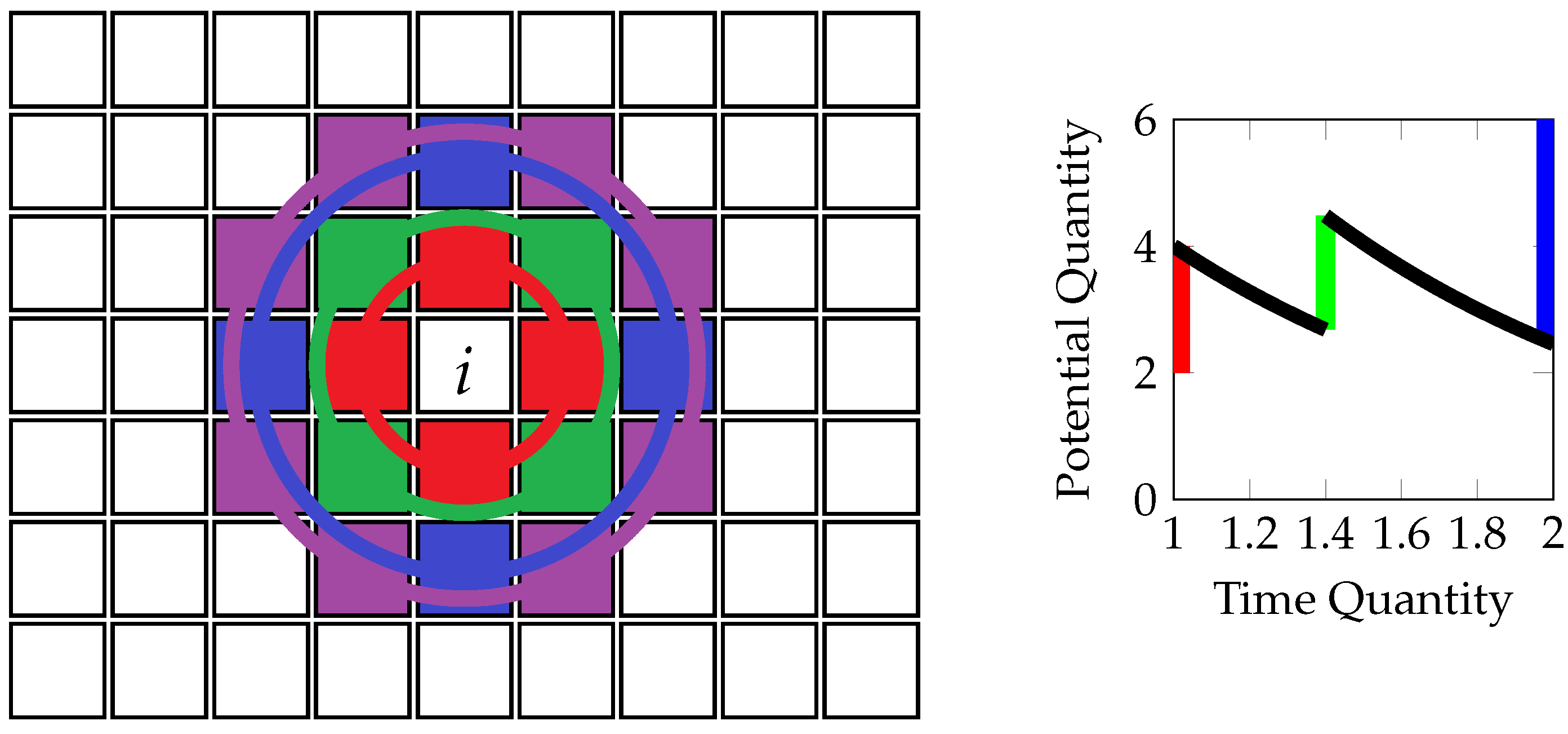
The code for Equation (6) is provided in the Appendix A such that $a_j$ is obtained readily sorted. As a third alternative, the same series is recovered with a rigorous derivation in the Appendix A. If the entire processing is supposed to be integrated into one neural net, then the computation of the input for the spiking neurons can be formulated as arithmetic neurons [13] fed by a layer which conducts a spline fit. Prior to the spline fit routine, survey data are curated by removing all soundings above the water surface. The functioning of a spiking neuron and particularly the circle-shaped arithmetic stimuli input is illustrated in Figure 1 below.

The pre-processing prior to identifying the neuron properties is conducted. Therefore, by eliminating all dry measurements m,

$$m=m^{*}(\forall m^{*}>0)$$

(7)

An input quantity is differentiated from an output quantity by the indication of a superscript asterisk. Measurements m, i.e., echo soundings, are then correlated with satellite image values v according to

$${\left.\sum _{dim=\left[12\right]}\left|x_{dim}^m-x_{dim}^v\right|\right|}_{min}$$

(8)

for the distance $x_{dim}$. Given the satellite image resolution of 30 m, measurements that share a pixel are averaged. Measurements that share the same pixel shade are averaged too. To ascertain that all depths are in each third and preclude an interference of the partition onto the results, elements are distributed to three equal parts in alternating fashion. That is, the first third comprising $[d_1{d}_4{d}_7\cdots ]$, the second $[d_2{d}_5{d}_8\cdots ]$ and so forth. Associated measurements and pixel shades are bookkept by referencing for a particular post-processing measurement the found post-processing pixel shading in the second layer. This is conducted for each color or band. For the third layer, the arithmetic neurons compute the input term in Equation (1). The SNN layer then processes the output depths further as per Equations (1) and (2), and

$$d=d^{*}(\forall f<f_{th})$$

(9)

with the threshold $f_{th}$. Pixels where the successive weighted deviations pass the threshold are deemed outlying and eliminated. The multiband fitting then utilizes unused echo measurement values to compute the best band weighting factor $w_i\in \mathbf{w}$ for a particular color i and pixel shading. The nonzero values for a particular vector $\mathbf{w}$ of weighing factors are, hence, given with

$$\begin{array}{cc}w\left(i_{min\left({\mathbf{d}}^{*}\right)}\right)=1,\hfill & \hfill \mathrm{for}{d}^m<min\left({\mathbf{d}}^{*}\right)\\ w\left(i_{max\left({\mathbf{d}}^{*}\right)}\right)=1,\hfill & \hfill \mathrm{for}{d}^m>max\left({\mathbf{d}}^{*}\right)\\ \begin{array}{c}{w}_a=\frac{d^m-d_b}{d_a-d_b}\hfill \\ \wedge w_b=\frac{d^m-d_a}{d_b-d_a}\hfill \end{array}\wedge \left[\begin{array}{c}a\\ b\end{array}\right]=\mathbf{i}\left(\notin i_{max\left({\mathbf{d}}^{*}\right)}\right),\hfill & \hfill \mathrm{for}\prod \left(d^m-{\mathbf{d}}^{*}\right)>0\\ \begin{array}{c}{w}_a=\frac{d^m-d_b}{d_a-d_b}\hfill \\ \wedge w_b=\frac{d^m-d_a}{d_b-d_a}\hfill \end{array}\wedge \left[\begin{array}{c}a\\ b\end{array}\right]=\mathbf{i}\left(\notin i_{min\left({\mathbf{d}}^{*}\right)}\right),\hfill & \hfill \mathrm{for}\prod \left(d^m-{\mathbf{d}}^{*}\right)<0\end{array}$$

(10)

$i_{min\left({\mathbf{d}}^{*}\right)}$ and $i_{max\left({\mathbf{d}}^{*}\right)}$ are the indices of the minimal and maximum depth estimates, respectively, from the three utilized bands. Equation (10) merely describes the different cases of weighting two adjacent depths out of three band estimates to return the measured depth. If the measured depth is above or below the highest and deepest estimates respectively, then only one band is used. If the measured depth lays between the first two or the last two of the three bands, then the former or the latter are picked to contribute to the weighting. Hence, Equation (10) contains four cases.

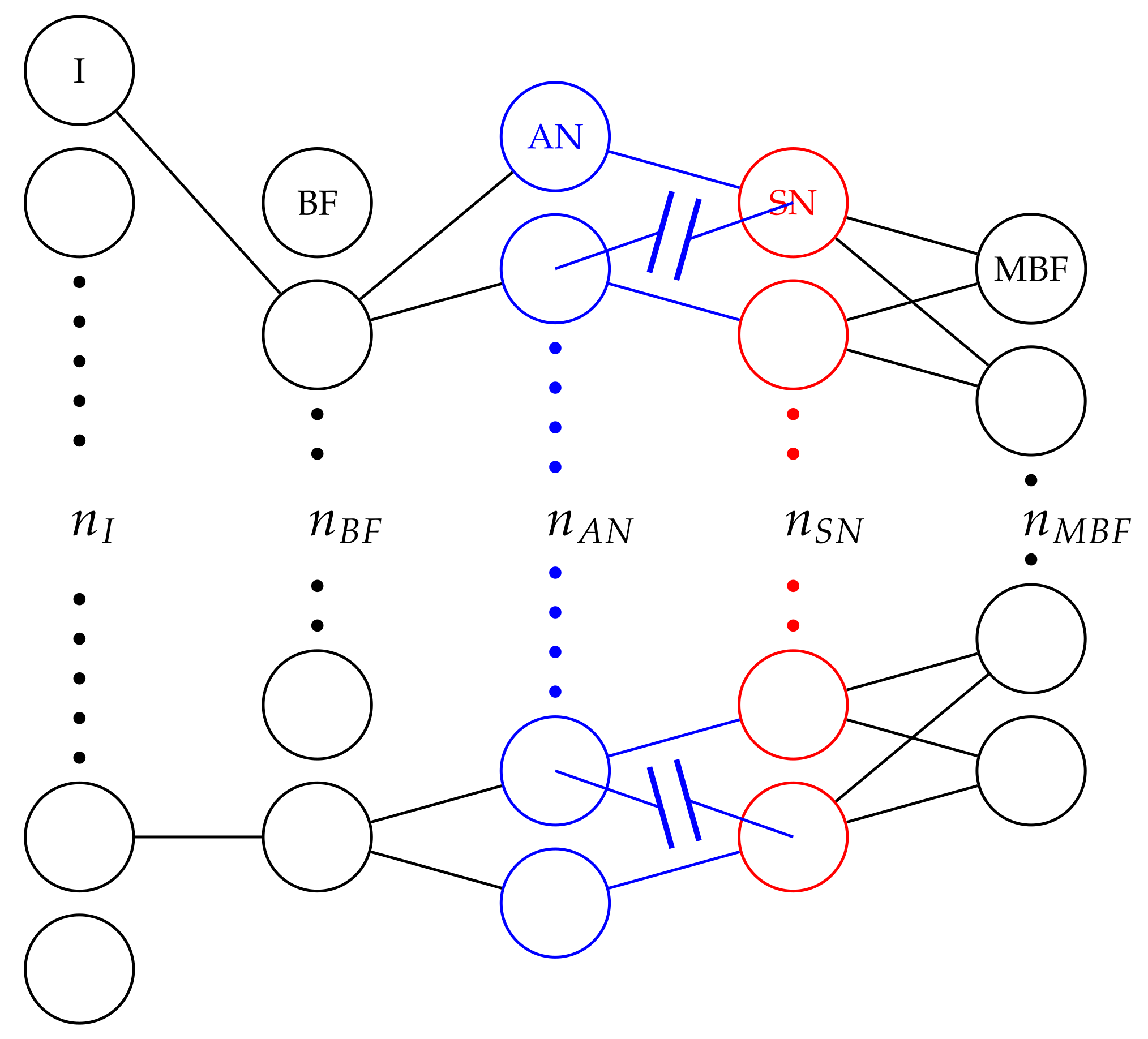
If all processing is cast into one neural net, then the synapses between the first and second layer conduct a spline fit, and the multi-band fitting post SN constitutes a bona fide neural layer, where several inputs vote with individual weighting factors. The intersected SN layer permits to exclude locally volatile pixel values which statistically correspond to an elevated probable error. The computational effort for the key spiking neuron anomaly detection depends on the cutoff radius within which neighboring pixels are taken into account. In actual application, the image size vastly exceeds the number of intertwined neighboring neurons. A fixed cutoff radius and, hence, fixed number of relevant neighboring pixels, entails thus a complexity of $O\left(n\right)$. The functions of the normal, arithmetic and spiking layers are illustrated in Figure 2 below.

Increasing spatial distance corresponds here to an increasingly delayed time of spike stimulation. The refinement of this conversion might warrant examining the conversion of still perception fields to transience in biological SNN and if this exploits the difference in transmission times of chemical vs. electrical synapses.

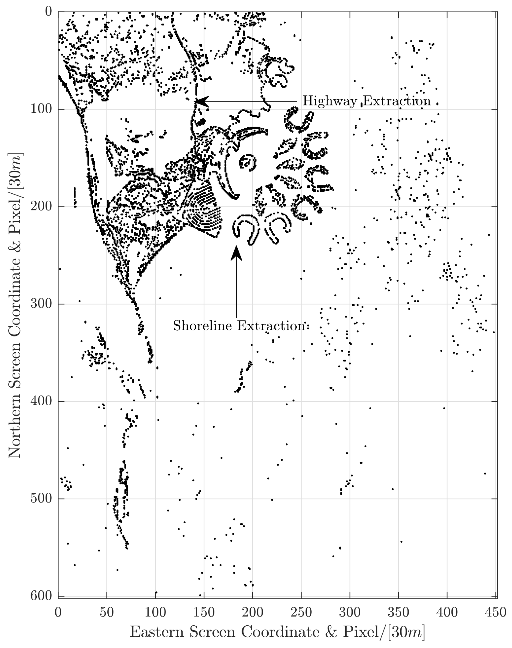
Based on parameter estimation iterations, the threshold of the neurons is set to 6 for error filtration. For method comparison, errors are computed against soundings retained for this accuracy examination. That is, the first third is used to conduct the spline fitting for all bands; the second third is used to assess the spline fittings’ errors before and after spiking neuron filtration and to conduct the weighting of bands; and the remaining third is used to estimate the error of the composite fitting before and after spiking neuron filtration. It occurs that if the arithmetic and SN layers are moved to the end of the stack, then features such as shorelines and highways are extracted. The output for this configuration is shown in Figure A1.

3. Results

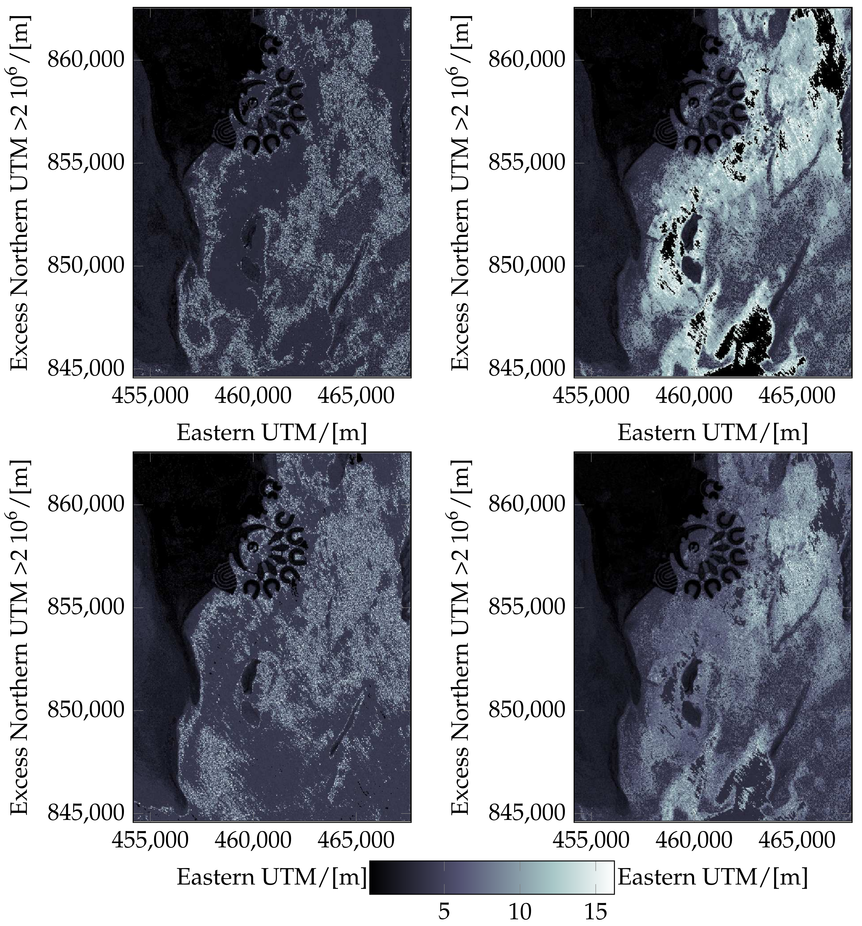
The method was tested by applying it to recreational and residential artificial islands at the coast of Bahrain. Survey bathymetry data were obtained for the Gulf of Salwa through echo sounding measurements that longitudinally extended from shallow to deeper sections. More than 30 thousand echo measurements were used, covering a depth up to 16 m. The bathymetry distributions obtained from satellite bands $B_2$ to $B_4$ and the final triband bathymetry distribution are shown in Figure 3 below. The three utilized Landsat 8 images, band 2 to 4, were recorded in March 2021 with 7631 × 7781 pixels at a resolution of 30 m. The triband bathymetry in the lower right corner exhibits a low error of 7.9% and high robustness, as all pixels are successfully converted into bathymetric estimates.

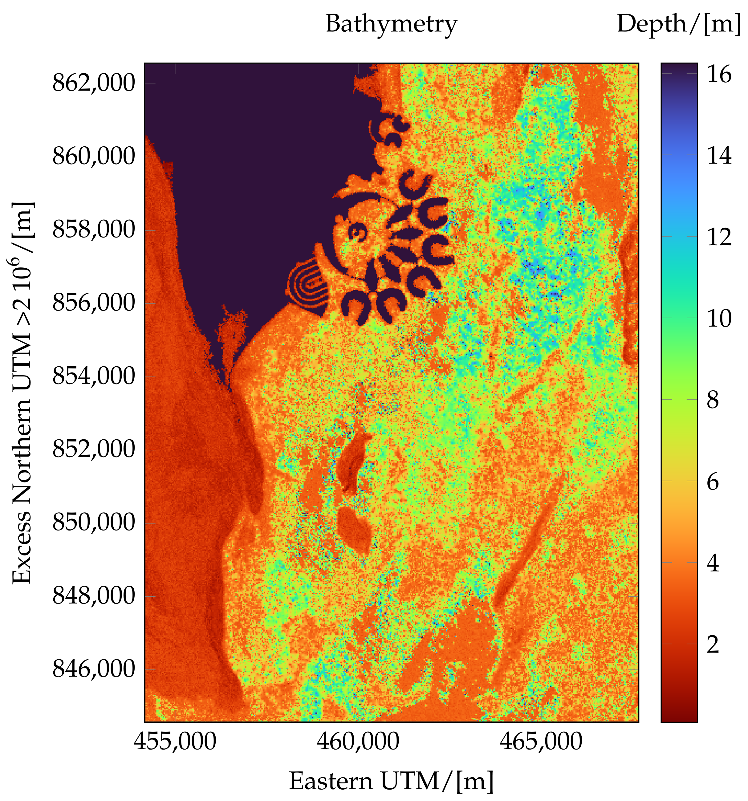
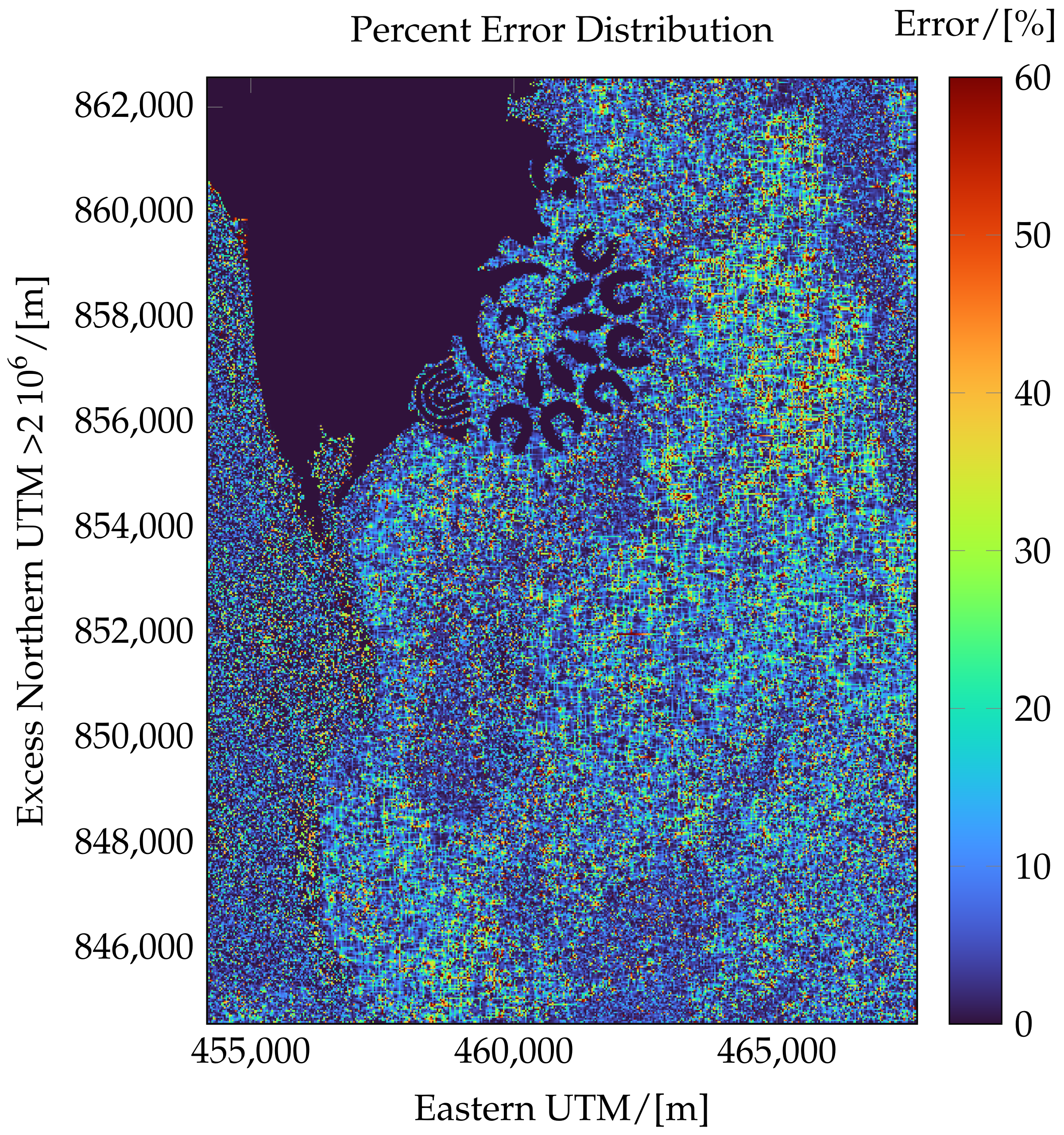
The quantities that determine the size of the neural layers are listed in

Table 1. Pixel properties.

Pixel Property	Case
$2^{\mathrm{bit}\mathrm{depth}}$	$2^{16}$
${\mathrm{depth}}_{\max }\times$ resolution/[m]	$16.5\times {10}^2$
horizontal number	7631
vertical number	7781
locally proximate: $1+3\times 2^2+2^3+\cdots$	here:21

below. Outliers have subsequently been filtered, reducing the error as shown for the composite sensing in Figure 4. The refined, displayed in Figure 5, exhibits a common smooth area at the left and uneven areas in front of the artificial islands.

The filtered multi-band fitting with shore recognition is shown in Figure 5. The settled silt is visible on the uniformly dredged floor of the artificial island development.

Depths at less than 2 m are additionally error-prone due to tidal and wave dynamics. As the water column’s relative transience is significant in shallow sections, the local reflectively is then increasingly ill-posed. For example, in intertidal wet–dry zones and at centimeter scales, the local relative error inherently spans the entire water column.

Figure 4 below shows the error distribution for the first 1000 measurements for the composite sensing and the spiking neuron filtered result. Figure 4 appears to confirm the premise that a low baseline error is compromised by error outliers that exceed the former by logarithmic orders of magnitude. The detection of the latter is, thus, relevant to the refinement of the sensing.

The accuracy was assessed based on the average of all percent errors relative to soundings retained for error computation:

$$error=\overline{\frac{\left|d^m-d^{TB}\right|}{d^m}}100$$

(11)

One third of the entire survey was utilized for the error estimation. Each error is the normalized difference between the triband sensed depth $d^{TB}$ and measurements $d^m$. The percent average errors are listed in

Table 2. Percent Average Errors.

	Band 2	Band 3	Band 4	Composite
Unfiltered	$19.719$	$7.283$	$14.920$	$7.932$
Filtered	$19.608$	$7.081$	$14.696$	$7.917$

below. The average error $7.9\%$ for the filtered composite fitting translates to 0.253 m. Whereas the limited resolution of the Landsat satellite, that is, 30 × 30 m, provides an inherent smoothing, high resolution commercial satellite images might benefit more from the SNN anomaly detection. The accuracy of the composite fitting is high enough to conduct a reliable automatic shoreline recognition with a flood fill algorithm. That is, the algorithm propagates from the deepest smoothed average and halts at pixels that are shallower than the cutoff depth.

The dense infrastructure in artificial islands and streets in proximity to the shore required a deeper cutoff than natural shores, that is, because dark shaded streets can be mistaken for water in Landsat bands 2 to 4. The filtered composite fitting with automatically excised land is depicted in Figure 5. Despite the low image resolution of 30 m, four circular channels were resolved west of the artificial islands such that also the shoreline could be resolved for each channel. Sensing of band 3 provided the lowest average error. The composite solution reduced incidences of high errors by evening the resulting error distribution, eliminated unprocessed pixels, and retained an average error similar to the best band. The leveling effect is evident when comparing the average errors for the filtered sensing of band 3 and the composite: whereas the former is refined in the second digit, the latter is refined only in the third digit.

An error distribution is estimated by mapping the errors for certain depths to the best matching depths in Figure 6.

4. Discussion

The tri-band fitting, in conjunction with spiking neurons, permitted to sense bathymetry with an average percent error of 7.9% or 25.3 cm. Stationary inputs can be processed by substituting time with spatial coordinates. The anomaly detection also underlined shorelines and roads, that is, object boundaries, as these are anomalies in terms of shading as shown in the Appendix B with Figure A1. The remote sensing was accurate enough to automatically excise land from sea. That is, shoreline recognition is possible via both vertical resolution or anomaly detection. Despite the low 30 m resolution of the Landsat image, improvements due to the anomaly detection were consistently found for all individual bands and the composite fitting.

Gains are expected to increase for the high resolution available with commercial satellite images, absent the inherent averaging of the limited resolution.

Conclusions

This bathymetric RS method is, to our knowledge, the first to involve spiking neuron anomaly detection, which contributed to achieve high accuracy, limiting the error to 25 cm. Unforeseen, despite the low Landsat 8 image resolution, this permitted also to ad hoc incorporate an automatic shoreline recognition with a flood fill algorithm that halts at dry pixels. Furthermore, the spiking neuron anomaly detection can operate on streamed time series, streamed array data, and, due to the generality of the SN concept, spatially unstructured array data. Further investigations may address the detection of anomalies in the sorted measurement series instead of vs. the seafloor and to smooth the weighting distribution beyond the current local weighting for each vertical increment. Especially the shoreline recognition can be further enhanced by incorporating the near infrared, for example, band 5 of Landsat 8, and bands that discern water based on a difference in thermal properties between wet and dry pixels. Onward, the automatic meshing for automated computer fluid dynamic simulations will be developed and published separately.

References

- Geyman, E.C.; Maloof, A.C. A Simple Method for Extracting Water Depth From Multispectral Satellite Imagery in Regions of Variable Bottom Type. Earth Space Sci. 2019, 6, 527–537. [Google Scholar] [CrossRef]
- Al Najar, M.; Thoumyre, G.; Bergsma, E.W.J.; Almar, R.; Benshila, R.; Wilson, D.G. Satellite derived bathymetry using deep learning. Mach. Learn. 2021, 1–24. [Google Scholar] [CrossRef]
- Mandlburger, G.; Kölle, M.; Nübel, H.; Soergel, U. BathyNet: A Deep Neural Network for Water Depth Mapping from Multispectral Aerial Images. PFG J. Photogramm. Remote Sens. Geoinf. Sci. 2021, 89, 71–89. [Google Scholar] [CrossRef]
- Collins, A.M.; Brodie, K.L.; Bak, A.S.; Hesser, T.J.; Farthing, M.W.; Lee, J.; Long, J.W. Bathymetric Inversion and Uncertainty Estimation from Synthetic Surf-Zone Imagery with Machine Learning. Remote Sens. 2020, 12, 3364. [Google Scholar] [CrossRef]
- Hong, D.; Han, Z.; Yao, J.; Gao, L.; Zhang, B.; Plaza, A.; Chanussot, J. SpectralFormer: Rethinking Hyperspectral Image Classification with Transformers. IEEE Trans. Geosci. Remote Sens. 2021, 60, 5518615. [Google Scholar] [CrossRef]
- Hong, D.; Gao, L.; Yokoya, N.; Yao, J.; Chanussot, J.; Du, Q.; Zhang, B. More Diverse Means Better: Multimodal Deep Learning Meets Remote-Sensing Imagery Classification. IEEE Trans. Geosci. Remote Sens. 2021, 59, 4340–4354. [Google Scholar] [CrossRef]
- Hong, D.; Yao, J.; Meng, D.; Xu, Z.; Chanussot, J. Multimodal GANs: Toward Crossmodal Hyperspectral–Multispectral Image Segmentation. IEEE Trans. Geosci. Remote Sens. 2021, 59, 5103–5113. [Google Scholar] [CrossRef]
- Yusob, B.; Mustaffa, Z.; Sulaiman, J. Anomaly Detection in Time Series Data Using Spiking Neural Network. Adv. Sci. Lett. 2018, 24, 7572–7576. [Google Scholar] [CrossRef]
- Verzilizi, S.J.; Vineyard, C.M.; Aimonel, J.B. Neural-Inspired Anomaly Detection; Technical Report SAND2018-5891C; Sandia National Laboratories: Albuquerque, NM, USA, 2018. [Google Scholar]
- Al-Ruzouq, R.; Shanableh, A. Multi-Temporal Satellite Imagery for Urban Expansion Assessment at Sharjah City /UAE. IOP Conf. Ser. Earth Environ. Sci. 2014, 20, 012010. [Google Scholar] [CrossRef]
- Cui, W.; Jia, Z.; Qin, X.; Yang, J.; Hu, Y. Multi-temporal Satellite Images Change Detection Algorithm Based on NSCT. Procedia Eng. 2011, 24, 252–256. [Google Scholar] [CrossRef] [Green Version]
- USGS. USGS Earth Explorer; U.S. Department of the Interior: Washington, DC, USA, 2021.
- Silver, R.A. Neuronal arithmetic. Nat. Rev. Neurosci. 2010, 11, 474–489. [Google Scholar] [CrossRef] [PubMed] [Green Version]
- Anderson, I. Reviews—An introduction to the theory of numbers (sixth edition), by G. H. Hardy and E. M. Wright. Pp. 620. 2008. (paperback). ISBN: 978-0-19-921986-5 (Oxford University Press). Math. Gaz. 2010, 94, 184. [Google Scholar] [CrossRef]
Figure 1.
(Left): increments among discrete distances (red, green, …) of neighboring pixels are (right) corresponding to time increments in the spiking activation.
Figure 2.
Layers with a number neurons for input (), band fitting (), arythmetics (), conventional neurons , arithmetic, and spiking neurons . Neuron numbers are indicated for the application case demonstrated in the subsequent section.
Figure 3.
Bathymetry in meters, sensing for band 2 (upper left), band 3 (upper right), band 4 (lower left), and a triband combination (lower right). The triband combination, shown in the lower right corner, is the most robust, free of unrecognized swathes.
Figure 4.
As outliers with high errors are filtered, the post-filtration series shifts left. Pre- and post-SN exhibit in this section, despite the outliers, moderate average errors of % and %, respectively. Additionally shown is the SN improvement in percent.
Figure 5.
SNN filtered bathymetry with automatically excised shoreline.
Figure 6.
Estimated error distribution surrounding the artificial islands.