Analysis of the Relative Importance of the Main Hydrological Processes at Different Temporal Scales in Watersheds of South-Central Chile

Abstract

In Chile in recent years, changes in precipitation and temperatures have been reported that could affect water resource management and planning. One way of facing these changes is studying and understanding the behavior of hydrological processes at a regional scale and their different temporal scales. Therefore, the objective of this study is to analyze the importance of the hydrological processes of the HBV model at different temporal scales and for different hydrological regimes. To this end, 88 watersheds located in south-central Chile were analyzed using time-varying sensitivity analysis at five different temporal scales (1 month, 3 months, 6 months, 1 year, and 5 years). The results show that the model detects the temporality of the most important hydrological processes. In watersheds with a pluvial regime, the greater the temporal scale, the greater the importance of soil water accumulation processes and the lower the importance of surface runoff processes. By contrast, in watersheds with a nival regime, at greater temporal scales, groundwater accumulation and release processes take on greater importance, and soil water release processes are less important.

1. Introduction

Due to climate change, climate variability, and changes in land use and cover, the frequency and magnitude of extreme events such as floods have continually increased in recent decades, generating environmental, economic, and social losses worldwide [1,2]. Thus, establishing a connection between watershed properties and climate and hydrological variables could illustrate the vulnerability of a watershed to various changes, thereby contributing to the development and management of systems that are resilient to natural disasters [3,4,5]. An important part of this development is the study of the dominant processes in a watershed and their temporality as, depending on the process, they could take on importance at different temporal scales—from minutes, hours (e.g., floods), weeks, and months to years (e.g., droughts)—and vary in wet and dry periods [6,7,8].

Analysis of the temporality of the most important processes that influence various climate scenarios has become a focus of study for many researchers. For example, Diop et al. [9] investigated the long-term streamflow trends at three time scales (monthly, seasonal, and annual) in the upper Senegal River basin, Howden et al. [10] presented a method to detect changes in the mean and variance of hydrological variables and explore the hydrological processes involved in the non-seasonal behavior of time series, and Basijokaite and Kelleher [11] analyzed the relationship between the most important processes in a watershed and their seasonal and annual behavior. In addition, various studies have demonstrated that changes in streamflow time series can be attributed to climate [12,13,14,15] and/or anthropogenic factors [16,17]. Thus, they provide important information for understanding the hydrological processes of a watershed and their different responses to changing climate conditions.

Analysis and understanding of hydrological processes and their changes depend on the sufficient availability of hydrometeorological information on a watershed. Thus, hydrological models are a fundamental component in the development of studies. They are also crucial for water resource planning and management, as they allow the simulation of streamflow series through a simplified representation of hydrological processes, providing a basis for understanding and investigating the relationship between the climate and water resources. In addition, complementary tools such as sensitivity analysis allow models to be evaluated to guarantee acceptable results and greater representativeness of these processes [18] through the study of the impact of input factor variation on model results [19,20,21]. Their application and understanding have increased in recent years, as they have become recognized as an essential tool for the development and assessment of environmental models [19,22,23]. Unlike traditional sensitivity analysis, which is based on model aggregation over time [24,25], time-varying sensitivity analysis (TVSA) allows the sensitivity to be estimated in a moving window; that is, the calculated value is assigned to the center of the window. This method helps identify the components that affect model performance, analyze their functioning, and obtain a more precise estimate of the factors [24,26,27]. Therefore, it allows the selection of a more suitable representation of a system for prediction in unmonitored watersheds and under changing conditions and the study of hydrological processes, their temporal variability, and their relationship with climate variables.

In recent years, various studies have reported a decrease in precipitation [28,29,30,31] and snow and glacier cover [32,33,34] and an upward temperature trend [35,36] in south-central Chile. In addition, since 2010 there has been a rainfall deficit in south-central Chile. This event, termed the megadrought, brought about a marked decrease in water reserves, contributing to an extended dry trend [30,37]. These changes could affect the way in which water is managed on a regional level for different uses, as well as for confronting extreme events such as floods and droughts. However, in Chile, streamflow records are relatively short (30 years on average), and stations are distributed unequally throughout the country [38,39], complicating the analysis of hydrological processes. Therefore, the objective of this study is to analyze the importance of the processes represented by the 10-parameter Hydrologiska Byråns Vattenbalansavdelning (HBV) hydrological model [40] at different temporal scales using information from watersheds with different hydrological regimes located in Chile.

2. Materials and Methods

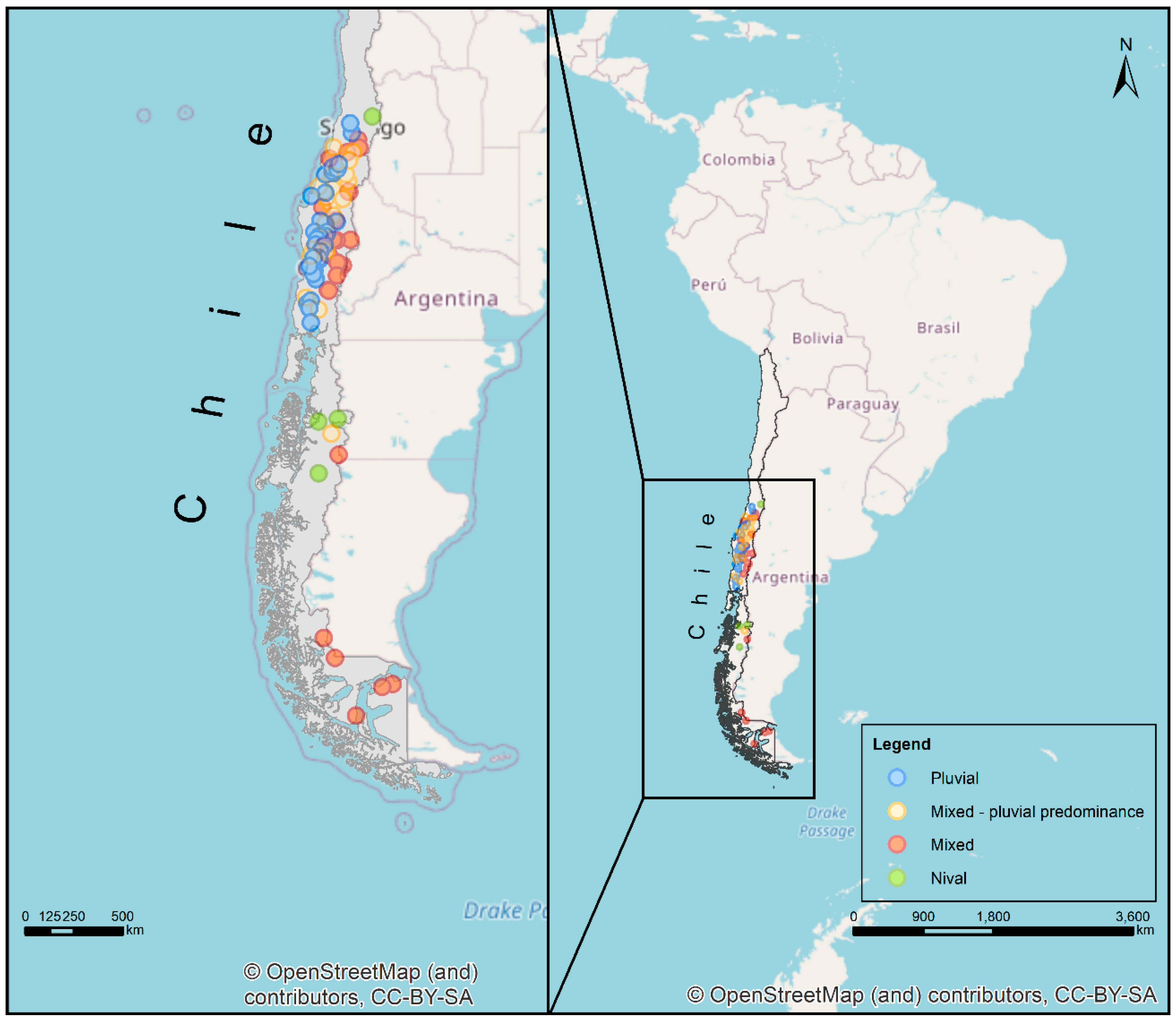
2.1. Study Area and Data

In addition to being important for human consumption, water resources are an essential part of the development of economic activities. Among the most important activities associated with water resources, both in Chile and the world, are industrial, mining, forestry, agricultural, and livestock activities, which vary in each zone depending on the climate conditions.

In order to avoid the influence of anthropogenic effects (e.g., reservoirs, canals, etc.) on the analysis, watersheds without (or with minimal) anthropogenic alternations and, since streamflow records have a relatively short length, with at least 30 years of daily records of hydrometeorological information, were selected. Thus, the study area consists of 88 watersheds located between latitudes 33°30′ S and 56°30′ S (Figure 1).

Central Chile (30°–40° S) presents a Mediterranean climate with mean annual precipitation that ranges from 100 to 3000 mm, distributed in a seasonal cycle characterized by an increase in precipitation in winter and very low values in summer. In the austral region (40°–56°30′ S) precipitation presents very wet conditions, reaching over 4000 mm per year, accompanied by strong winds throughout the year [41,42].

Due to the geographic units present throughout Chile (Andes Mountains, intermediate depression, coastal mountains, and coastal plains), river regimes are regulated by the climate, with intra-annual variability. Pluvial basins present precipitation seasonality, while snow–rain basins present intra-annual variability controlled by precipitation–snow accumulation and snowmelt/glacier melt processes controlled by temperature cycles in the Andes [43].

To determine the hydrological regime of each watershed, a flood frequency analysis was carried out. Of the 88 studied watersheds, 34 present a pluvial regime (P), 25 a mixed regime with pluvial input predominating (Mp), 25 a mixed regime (M), and 4 a nival regime (N). Rivers with a pluvial regime depend directly on winter rain (July–September) and have a period of low flows during the summer months (January–March). In rivers that present a mixed regime with rainfall predominance, the main input is winter rain (July–September), along with a minor contribution from snowmelt during the spring months (October–December). Unlike the previous regime, in mixed regime watersheds, the main contributions depend on rainfall and snow accumulation during winter and snowmelt in the spring–summer months. Finally, rivers with a nival regime are characterized by increased flows during the spring–summer periods (October to March) caused by snowmelt that depends on the increase in temperatures.

Table A1. Information on the 88 watersheds used in the study.

Station Code	Area (km2)	Lat. (°)	Altitude (masl)	Interv. Degree	Regime	Station Code	Area (km2)	Lat (°)	Altitude (masl)	Interv. Degree	Regime
5702001	523.4	−33.8	1304	0.029	Nival	9104001	93.8	−38.2	319	0.000	Pluvial
6018001	1022.6	−34.4	166	0.020	Pluvial	9104002	393.1	−38.2	266	0.005	Pluvial
6027001	349.4	−34.7	542	0.049	Mixto	9106001	276.7	−38.3	282	0.004	Pluvial
6043001	801.8	−34.1	118	0.228	Pluvial	9107001	853.6	−38.3	82	0.006	Pluvial
7103001	354.4	−35.0	664	0.020	Mixto	9113001	710.0	−38.4	26	0.061	Pluvial
7116001	367.2	−35.2	426	0.084	Mixto P	9116001	5047.6	−38.6	19	0.014	Pluvial
7123001	5699.9	−35.0	5	0.073	Mixto P	9122002	170.9	−38.5	551	0.031	Mixto
7330001	502.4	−36.4	275	0.005	Mixto P	9123001	1306.1	−38.4	413	0.005	Mixto
7332001	1209.0	−36.2	121	0.439	Mixto P	9127001	650.3	−38.6	158	0.001	Pluvial
7335001	1686.8	−36.1	103	0.460	Mixto P	9129002	2755.6	−38.7	115	0.006	Mixto
7335002	217.0	−36.0	103	0.070	Pluvial	9134001	348.0	−38.9	125	0.003	Mixto P
7336001	622.1	−36.0	134	0.145	Pluvial	9135001	1665.6	−38.9	39	0.017	Pluvial
7339001	1637.5	−35.9	102	0.438	Pluvial	9140001	5547.3	−38.8	10	0.022	Mixto P
7343001	404.3	−35.8	134	0.309	Pluvial	9404001	1675.1	−39.0	205	0.022	Mixto
7350001	668.9	−36.2	449	0.003	Mixto P	9412001	356.9	−39.4	382	0.008	Mixto
7350003	466.9	−36.3	607	0	Mixto P	9414001	1379.4	−39.3	363	0.006	Mixto
7354002	894.3	−36.0	309	0.009	Mixto P	9416001	349.0	−39.3	277	0.019	Mixto
7357002	7078.8	−35.8	87	0.420	Pluvial	9433001	153.5	−39.2	81	0.005	Pluvial
7359001	9923.7	−35.6	65	0.255	Pluvial	9434001	769.7	−39.1	76	0.010	Pluvial
7372001	703.0	−35.2	155	0.068	Mixto	9436001	383.9	−39.1	26	0.018	Pluvial
7374001	382.3	−35.5	241	0.076	Mixto P	9437002	7926.8	−39.0	9	0.042	Mixto P
7383001	20514.6	−35.4	7	0.219	Mixto	10102001	367.9	−39.7	222	0.001	Mixto
8104001	606.7	−36.7	683	0	Mixto	10121001	626.2	−39.9	16	0.090	Pluvial
8105001	1254.3	−36.7	645	0.258	Mixto	10134001	1802.6	−39.6	14	0.040	Pluvial
8114001	970.1	−36.6	108	0.001	Mixto P	10137001	539.0	−39.7	8	0.031	Pluvial
8123001	860.1	−37.2	206	0.003	Mixto P	10140001	107.6	−39.4	10	0.019	Pluvial
8124001	1661.9	−36.9	79	0.002	Mixto P	10304001	1725.8	−40.3	55	0	Mixto
8124002	1148.2	−37.1	154	0.003	Mixto P	10306001	308.6	−40.3	125	0.093	Mixto
8130002	204.4	−36.9	715	0	Mixto P	10343001	313.3	−40.9	159	0.002	Mixto P
8132001	1300.5	−36.9	68	0.029	Mixto P	10356001	2279.7	−40.7	26	0.044	Pluvial
8134003	636.1	−36.7	42	0.004	Pluvial	10362001	466.8	−40.6	34	0.054	Pluvial
8135002	4510.0	−36.7	23	0.015	Mixto P	10363002	169.0	−40.9	84	0.041	Pluvial
8141001	10405.2	−36.5	24	0.110	Mixto P	10364001	5603.0	−40.5	7	0.038	Mixto P
8220001	750.3	−36.8	8	0.034	Pluvial	10411002	253.2	−41.4	44	0.089	Pluvial
8304001	466.7	−38.4	870	0.004	Mixto	11143001	2258.4	−44.7	465	0.004	Nival
8317001	7252.5	−37.7	257	0.004	Mixto	11143002	133.9	−44.8	484	0	Nival
8317002	103.4	−37.8	333	0.004	Pluvial	11302001	1997.0	−45.2	136	0.046	Mixto P
8323002	817.7	−37.6	230	0.003	Mixto P	11310001	1143.1	−45.8	482	0.145	Mixto
8342001	688.2	−37.9	118	0.009	Mixto P	11514001	897.1	−46.4	215	0	Nival
8343001	440.2	−37.9	120	0.011	Pluvial	12285001	101.1	−51.5	160	0	Mixto
8351001	415.1	−38.0	147	0	Pluvial	12582001	864.0	−53.7	4	0	Mixto
8358001	2537.0	−37.7	47	0.009	Pluvial	12600001	504.4	−52.0	183	0	Mixto
8383001	3428.2	−37.2	61	0.006	Mixto	12802001	808.5	−52.8	39	0	Mixto
9102001	853.1	−38.2	47	0.002	Pluvial	12805001	559.6	−52.8	30	0	Mixto

presents a brief description of the watersheds used in the study.

To implement the hydrological model of each watershed considering data availability and to represent the current state of each system, precipitation, temperature, and evapotranspiration time series from 1990–2019 were used, obtained from the Catchment Attributes and Meteorology for Large Sample Studies—Chile Dataset (CAMELS-CL) presented by Alvarez-Garreton et al. [38], which comprises physical and hydrometeorological information from throughout Chile. In addition, streamflow records were used to perform the frequency analysis and carry out subsequent analyses. It bears mentioning that the information obtained from the CAMELS-CL database can be used directly without applying data processing methods.

2.2. Model Description

The HBV model is a lumped conceptual snow–rainwater balance model. In this study, the simplified version developed by Aghakouchak and Habib [40] and based on Bergström [44] was used. The model simulates daily discharge based on daily precipitation, temperature, and potential evapotranspiration time series [40] and includes a snow routine, a soil routine, and a response routine (see conceptual diagram in Figure 2).

Precipitation is deemed to be snow or rain depending on the temperature on the corresponding day above or below a threshold temperature (TT). All precipitation is snow when the temperature is below TT, and all the snow contributes directly to the snow storage. If the actual temperature is greater than TT, there will be snowmelt. Snowmelt water is controlled by a degree–day factor (Cmelt), which determines the daily amount of melted snow depending on the difference between the actual and threshold temperatures. Subsequently, the sum of precipitation and snowmelt (ΔP) passes to the soil routine, which includes two modules. The first module calculates the actual evapotranspiration (ET_a), which is equal to potential evapotranspiration (PET_d) if the relationship between soil moisture (SM) and field capacity (FC) is above a threshold value for potential evapotranspiration (LP). However, for soil moisture values below LP, the actual evapotranspiration will be linearly reduced.

To calculate evapotranspiration, Bergström [44] introduced a routine that incorporates a correction factor (c) to obtain daily potential evapotranspiration (PET_d) from the daily mean air temperature and the long-term PET and monthly temperature averages.

Subsequently, the model calculates runoff (ΔQ), which depends on precipitation (ΔP), the actual water content of the soil (SM), the maximum soil moisture (FC), and an empirical coefficient (β), which determines the relative contribution of rain or snowmelt to runoff. Finally, the runoff response routine estimates the runoff at the watershed outlet. The system consists of two storage compartments, one above the other, which are directly connected to each other through a constant infiltration rate (Q_p).

The upper deposit has two outlets (Q₀ and Q₁), while the lower deposit has one (Q₂). When the water level in the upper deposit exceeds a threshold value (L), runoff is produced quickly in its upper part (Q₀). The response of the other outlets is relatively slow. The streamflows are controlled by recession coefficients K₀, K₁, and K₂, which represent the response functions of the upper and lower deposits. The constant infiltration rate (Q_p) is controlled by a coefficient K_p.

In order to ensure that the surface runoff process is quicker than the subsurface and groundwater runoff, the initial value of K₀ must always be greater than K₁. In addition, the response of the third outlet (groundwater runoff; Q₂) must be slower than that of the second one (Q₁); therefore, K₂ must be lower than K₁ [40]. For a better understanding of the model, see Bergström [44], Lindström et al. [45], and Seibert [46].

To adequately represent the spatial variability of precipitation and include the orographic effects in the study watersheds, a precipitation adjustment factor (A) was considered in the models. This factor allows the model to obtain a long-term mass balance [21] and thereby correct the underestimation of precipitation resulting from the absence of records in the highest parts of each watershed.

Table 1. Model parameters and initial ranges used for the analysis.

Parameter	Description	Range
	Mass balance
A	Precipitation modification parameter	0.8–2.5
	Snow module
TT (°C)	Threshold temperature that indicates the initiation of snowmelt (normally 0 °C)	0
Cmelt (mm °C−1 day−1)	Fraction of snow that melts above the threshold temperature (TT) from the beginning of snowmelt.	0.5–7
	Moisture module
FC (mm)	Field capacity (storage in the soil layer)	0–2000
Beta	Empirical coefficient that represents the soil moisture variation in the area	0–7
LP	Fraction of field capacity to calculate the permanent wilting point (PWP = LP × FC)	0.3–1
c(°C−1)	Correction factor for potential evapotranspiration	0.01–0.3
	Response module
L (mm)	Threshold for quick runoff response	0–100
${\mathrm{K}}_0$$({\mathrm{day}}^{-1}$)	Quick response coefficient (upper reservoir)	0.3–0.6
${\mathrm{K}}_1$$({\mathrm{day}}^{-1}$)	Slow response coefficient (upper reservoir)	0.1–0.2
${\mathrm{K}}_2$$({\mathrm{day}}^{-1}$)	Lower reservoir response coefficient	0.01–0.1
${\mathrm{K}}_{\mathrm{p}}$$({\mathrm{day}}^{-1}$)	Maximum flow coefficient for percolation	0.01–0.1

presents a brief description of the parameters and initial ranges used, based on the studies of Aghakouchak and Habib [40] and Kollat et al. [47].

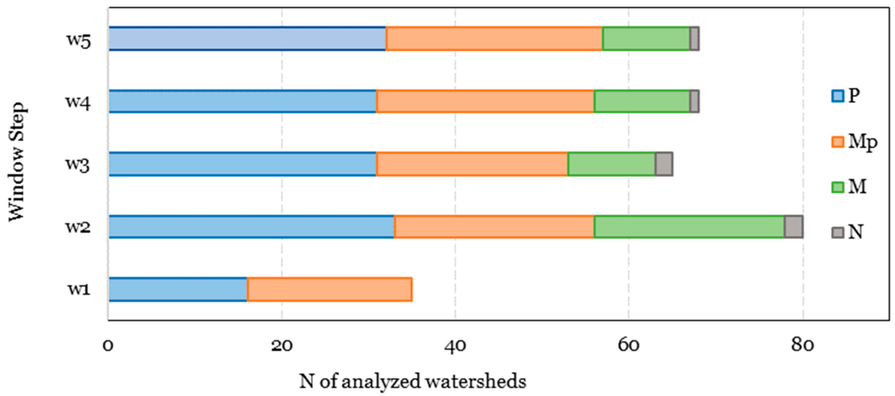
2.3. Description and Implementation of TVSA

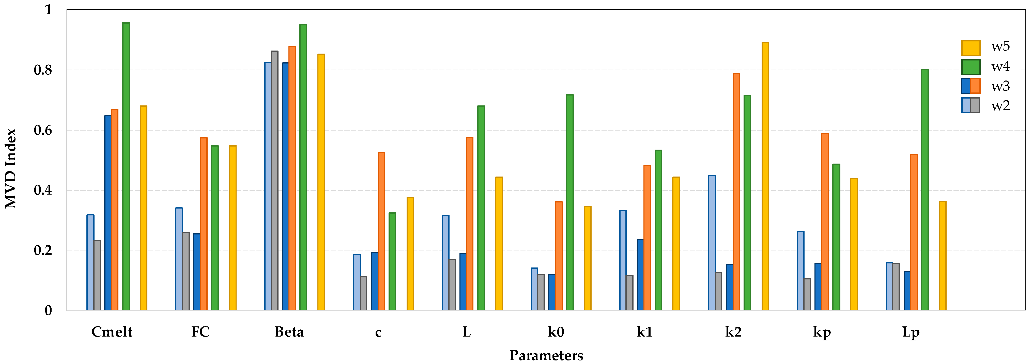
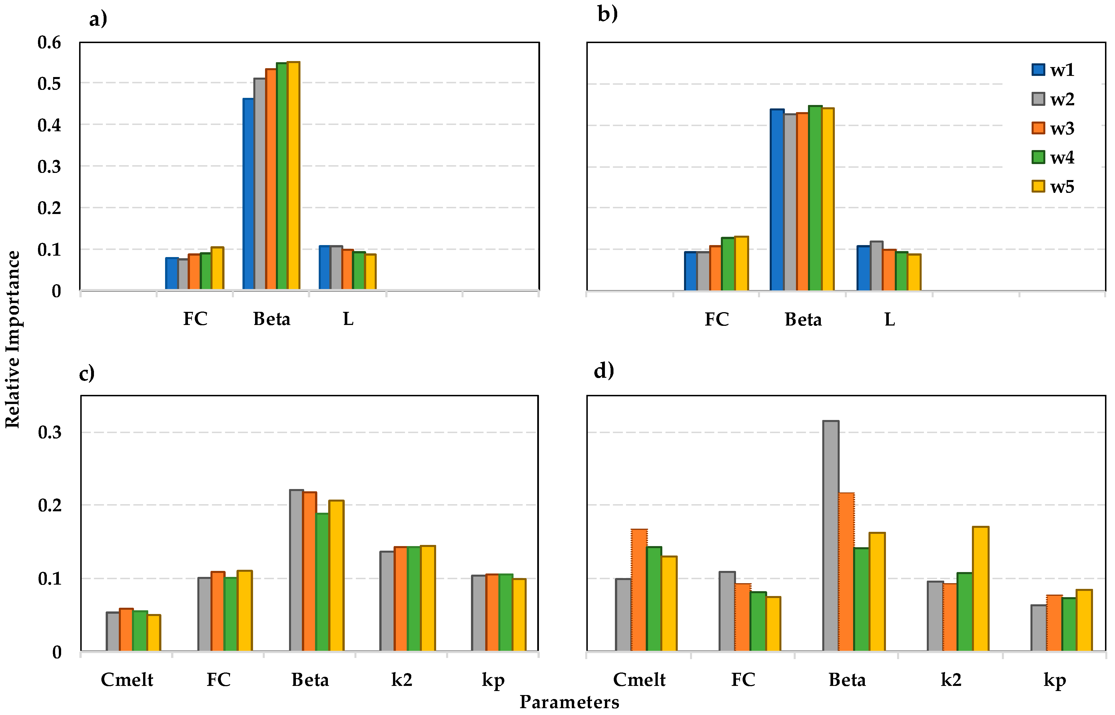
Through the estimation of sensitivity in a moving window, TVSA aids the identification of time periods in which a specific component of a model can affect its performance and uses additional information to analyze the functioning of the model and obtain a more precise estimate of the factors [6,24,25,26,27].

In this study, the code presented by Medina and Muñoz [27], which is based on Regional Sensitivity Analysis (RSA) [50], was used. It allows the most important hydrological processes in a watershed to be detected [49] and the factors to be ordered according to their relative influence on the model results (i.e., ranking) [20,49].

The method consists of generating a sample of N points in the feasible space of each parameter (x_i) obtained from a uniform distribution. The parameter sets are categorized as behavioral and non-behavioral (B and NB, respectively) based on an objective function. The cumulative distribution functions—${\mathrm{F}}_{\mathrm{i}}^{\mathrm{B}}\left({\mathrm{x}}_{\mathrm{i}}\right)$ and ${\mathrm{F}}_{\mathrm{i}}^{\mathrm{NB}}\left({\mathrm{x}}_{\mathrm{i}}\right)$—of both groups are compared and the discrepancy between them is quantified using, as a sensitivity index, the maximum vertical distance (MVDi) between the curves. The values of Equation (1) vary between 0 and 1. When the parameter sets do not generate B or NB models, the index cannot be calculated [27].

$${\mathrm{MVD}}_{\mathrm{i}}=\underset{{\mathrm{x}}_{\mathrm{i}}}{\max }\left|{\mathrm{F}}_{\mathrm{i}}^{\mathrm{B}}\left({\mathrm{x}}_{\mathrm{i}}\right)-{\mathrm{F}}_{\mathrm{i}}^{\mathrm{NB}}\left({\mathrm{x}}_{\mathrm{i}}\right)\right|,$$

(1)

To implement the TVSA, a Monte Carlo sampling of 15,000 simulations in the feasible space of each parameter was performed, assuming a uniform distribution. Five instances of TVSA were run, using windows of 1 month (w1), 6 months (w2), 1 year (w3), 3 years (w4), and 5 years (w5), with respective analysis periods for the calculation of the time-varying sensitivity analysis of 3 months, 8 months, 3 years, 6 years, and 9 years. Time windows are selected with the aim of detecting the hydrological processes that govern the main behavior of each watershed at different temporal scales, encompassing seasonality and longer-term processes such as climate variability. In addition, the five analyses allow the performance of the HBV model to be assessed at different time scales.

To calculate the MVD sensitivity index, it is necessary to group the simulations as B and NB. In this study, the Kling Gupta Efficiency (KGE) was used. The KGE index is focused on equitably assessing the correlation, deviation, and variability of the simulated hydrograph [51]; it is calculated with Equation (2):

$$\mathrm{KGE}=1-\sqrt{\left(\mathrm{r}-1\right)+\left(\mathsf{\alpha }-1\right)+\left(\mathsf{\beta }-1\right)}$$

(2)

where $\mathrm{r}$ is the linear correlation coefficient between the observed and simulated values, $\mathsf{\alpha }$ measures the variability of the data values (equal to the ratio between the standard deviation of the simulated data and the standard deviation of the observed data), and $\mathsf{\beta }$ is the ratio between the average of the simulated data and the average of the observed data. In the literature, the threshold value for a model to be considered adequate is KGE = 0.6 [52]. Therefore, the models that present KGE values equal to or greater than 0.6 were considered B, while models with KGE values below 0.6 were considered NB.

3. Results

The TVSA method based on RSA was implemented using simulations of 88 previously selected watersheds, and 5 analyses were performed at different time scales (1 month, 6 months, 1 year, 3 years, and 5 years). To calculate the MVD index, it is necessary that B (KGE ≥ 0.6) and NB (KGE < 0.6) results be obtained for the watershed model and time window. In some cases (watersheds), B solutions were not obtained; therefore, no solution in the analyzed time window was obtained.

Figure 3 shows the number of studied watersheds for which results (MVD index values for each parameter) were obtained in each analysis. In the analysis in which a time window of 1 month (w1) was used, fewer results were obtained (35 watersheds) in comparison to the other analyses. For w2 = 6 months, the greatest quantity of watersheds with solutions was obtained (80), while for w3, w4, and w5 (1, 3, and 5 years, respectively), a similar number of solutions was obtained (65, 68, and 68, respectively). In Figure 3, it is also observed that in the w1 analysis, no solutions for watersheds with a mixed or nival regime were obtained, while at least one was obtained in the other analyses (w2, w3, w4, and w5).

For subsequent analyses, the results of each time window using watersheds for which solutions were obtained were used.

Figure 4 and Figure 5 show the MVD sensitivity index calculated for each parameter in the different analyzed time windows (w1, w2, w3, w4, and w5). The number of analyzed watersheds with a nival regime (1 or 2, depending on the time window) did not allow the results to be grouped in a boxplot; therefore, they are shown individually in Figure 5. Figure 4a shows the results of watersheds with a pluvial regime, Figure 4b shows the results of watersheds with a mixed regime with pluvial predominance, and Figure 4c shows the results of watersheds with a mixed regime. In Figure 4a (pluvial regime), it is observed that the most sensitive parameters are Beta, FC, and L. Beta represents the variation of soil moisture, FC represents the maximum moisture capacity of the soil, and L defines the limit for a quick response (surface flow). Similarly, it is observed in Figure 4b (mixed regime with pluvial input predominating) that the most sensitive parameters are Beta, FC, and L, but it is also observed that the parameters related to groundwater—k2 and kp—present a slight relative increase in the range of MVD index values compared to the results of the watersheds with a pluvial regime. Meanwhile, in Figure 4c (mixed regime), a comparison with the results of the watersheds with pluvial predominance shows an increase in the range of MVD index values in all parameters except Beta, which remains the most sensitive parameter. It is also observed that, according to the median of the values, the parameters k2 and kp take on greater importance than in the watersheds with a pluvial regime. In Figure 5 (nival regime), unlike in Figure 4, it is observed that the model is more sensitive to the parameters Beta, Cmelt, and k2. Cmelt represents the fraction of snow that melts.

In the cases of the watersheds in Figure 4a, the main input is pluvial; therefore, soil moisture is the process that takes on the greatest importance in the model. Because these watersheds do not present a nival input, the model is not sensitive to the parameter Cmelt associated with snow accumulation and melting processes. Although the watersheds in Figure 4b present a nival regime influence, the pluvial input predominates and therefore major importance of the snow accumulation and melting process (Cmelt) is not detected. However, the analysis does allow an increase in the relative importance of processes associated with slow flows or baseflow (k2 and kp) to be detected. The watersheds in Figure 4c have a greater nival input than the watersheds in Figure 4a,b, which in this case allows the model to detect the importance of snowmelt and underground processes. This occurs because streamflows during low-water periods depend mainly on groundwater input.

It can also be seen in Figure 4 that the value range of the median MVD index of the parameter FC increases as the analyzed time window increases, and in the parameter Beta, the median MVD index exceeds values of 0.6 in all cases and different time windows.

Figure 6 shows the relative importance of the most sensitive parameters identified in watersheds with solutions for each analyzed time window. It was calculated for each parameter using the ratio of the sensitivity of a parameter to a set of corresponding parameters, that is, the value of the MVD index of the analyzed parameter over the sum of the MVD index of the complete parameter set. In Figure 6a (watersheds with a pluvial regime), it is observed that the relative importance of the parameters Beta and FC increases as the analyzed time window increases, while the relative importance of the parameter L decreases as the time window increases.

In Figure 6b (watersheds with a mixed regime with pluvial predominance), the same trends seen in Figure 6a are observed, except for parameter Beta, which does not present a significant change between the different temporal scales.

Figure 6c,b shows the relative importance of the most sensitive parameters in watersheds with mixed and nival regimes, respectively: Cmelt, FC, Beta, k2, and kp. In both figures, it is observed that the relative importance of the parameter Beta decreases as the analysis window increases, as is the case with Cmelt and FC in watersheds with a nival regime. By contrast, the relative importance of parameters k2 and kp increases in watersheds with a nival regime, and in watersheds with a mixed regime there are no differences in the relative importance of parameters Cmelt, FC, k2, and kp at the different temporal scales.

Parameters Beta and FC represent the variation of soil moisture and maximum soil moisture, respectively. It is observed that at, a greater temporal scale, soil water accumulation processes take on greater relative importance in watersheds with pluvial predominance. However, in watersheds with a mixed regime, this trend is not observed, and in watersheds with a nival regime, the opposite trend is seen, while processes of water accumulation and release from the aquifer (k2 and kp) take on greater relative importance in watersheds with a nival regime at greater temporal scales. By contrast, the relative importance of parameter L (the limit for surface runoff) decreases at greater temporal scales, as the surface runoff process acts in short time periods. In watersheds with a nival regime, streamflows depend mainly on snowmelt, a process that occurs in short time periods in which temperatures increase, such that at greater temporal scales its relative importance decreases. Because soil moisture and its variation depend on snowmelt, the importance of these processes follows the same trend (it decreases at greater temporal scales). Meanwhile, the relative importance of the parameters that represent the groundwater input (k2 and kp) increases at greater temporal scales since, unlike surface runoff, they are considered slow processes. These results are consistent with prior studies such as those presented by Medina and Muñoz [49], who conclude that the HBV model detects the most important processes in watersheds with different hydrological regimes, and Taucare et al. [53], who note the important input to aquifer recharge allowed by groundwater drainage from the Andes Mountains.

While the model allows the importance of hydrological processes and their temporality in watersheds with different hydrological regimes to be detected, it is not possible to simulate the processes of a watershed with a nival regime or with significant snowmelt input (mixed regime) at small temporal scales due to the limited sample of watersheds with these characteristics and the non-convergence of solutions for the calculation of MVD. This is observed in Figure 4c and Figure 5, as no results were obtained for the analysis with a one-month time window.

In general, it is observed that pluvial watersheds make up the majority in south-central Chile, where it is observed that processes related to soil water accumulation such as soil moisture variation and maximum soil moisture predominate in streamflow generation and take on greater importance as the analyzed time window increases.

In watersheds with a mixed regime, located throughout the central, southern, and austral zones, behavior similar to that of watersheds with pluvial input is observed, but processes of snowmelt and groundwater input also take on importance in streamflow generation, and trends regarding the variation of time windows are less clear.

Finally, in watersheds with a nival regime, located mainly in the austral zone of Chile, it is observed that streamflows depend on groundwater input, the importance of which increases in larger time windows, and soil moisture and snowmelt processes, the importance of which decreases at greater time scales.

4. Conclusions

Using the 10-parameter HBV model, time-varying sensitivity analysis (TVSA), and time windows of 1 month, 6 months, 1 year, 3 years, and 5 years, the relative importance of hydrological processes in 88 watersheds with different hydrological regimes located mostly in south-central Chile was analyzed.

In accordance with the obtained results, TVSA allowed the importance of HBV model parameters to be detected and the predominant hydrological processes of watersheds grouped by the hydrological regime to be identified. In all watersheds, the most sensitive parameter was Beta, which allows the process of water accumulation and release from the soil to be simulated, even in watersheds with a nival regime. In watersheds with pluvial predominance, the most important parameters were those that represent soil moisture (Beta and FC), while in watersheds with a greater nival input, the most sensitive parameters were those that represent the snow accumulation and melting process (Cmelt) and groundwater input (k2 and kp). Therefore, the model parameters that presented the greatest sensitivity were directly related to the hydrological regimes of the watersheds and their predominant hydrological processes. In addition, the model detects the temporality of the most important hydrological processes. In watersheds with a pluvial regime, at greater temporal scales, soil water accumulation processes take on greater importance and surface runoff processes take on less importance. Meanwhile, in watersheds with a nival regime, at greater temporal scales, the importance of processes of groundwater accumulation and release increases and the importance of soil water release decreases.

Due to the low number of watersheds with a nival regime and the limited convergence of B models, it was not possible for the model to simulate processes in watersheds with significant snowmelt inputs at small time scales of one month.

In addition, because the model is capable of simulating hydrological processes at different time scales and the TVSA tool detects the most/least relevant ones, it can be concluded that this method would allow the identification of possible alterations in the temporal distribution of the hydrological processes of a watershed, such as anticipated snowmelt, increased evapotranspiration, and changes in groundwater discharges, making it an important contribution to the development of research focused on climate change impacts and predictions and the management of resilient systems.

References

1. Buendia, C.; Batalla, R.J.; Sabater, S.; Palau, A.; Marcé, R. Runoff Trends Driven by Climate and Afforestation in a Pyrenean Basin. Land Degrad. Dev. 2015, 27, 823–838. [Google Scholar] [CrossRef] [Green Version]
2. Sharma, P.J.; Patel, P.; Jothiprakash, V. Impact of rainfall variability and anthropogenic activities on streamflow changes and water stress conditions across Tapi Basin in India. Sci. Total Environ. 2019, 687, 885–897. [Google Scholar] [CrossRef] [PubMed]
3. Birsan, M.-V.; Molnar, P.; Burlando, P.; Pfaundler, M. Streamflow trends in Switzerland. J. Hydrol. 2005, 314, 312–329. [Google Scholar] [CrossRef]
4. Raikes, J.; Smith, T.F.; Jacobson, C.; Baldwin, C. Pre-disaster planning and preparedness for floods and droughts: A systematic review. Int. J. Disaster Risk Reduct. 2019, 38, 101207. [Google Scholar] [CrossRef]
5. Quesada-Montano, B.; Di Baldassarre, G.; Rangecroft, S.; Van Loon, A.F. Hydrological change: Towards a consistent approach to assess changes on both floods and droughts. Adv. Water Resour. 2018, 111, 31–35. [Google Scholar] [CrossRef]
6. Guse, B.; Reusser, D.E.; Fohrer, N. How to improve the representation of hydrological processes in SWAT for a lowland catchment—temporal analysis of parameter sensitivity and model performance. Hydrol. Process. 2013, 28, 2651–2670. [Google Scholar] [CrossRef]
7. Reusser, D.E.; Buytaert, W.; Zehe, E. Temporal dynamics of model parameter sensitivity for computationally expensive models with the Fourier amplitude sensitivity test. Water Resour. Res. 2011, 47. [Google Scholar] [CrossRef] [Green Version]
8. Cristiano, E.; ten Veldhuis, M.-C.; van de Giesen, N. Spatial and temporal variability of rainfall and their effects on hydrological response in urban areas—A review. Hydrol. Earth Syst. Sci. 2017, 21, 3859–3878. [Google Scholar] [CrossRef] [Green Version]
9. Diop, L.; Bodian, A.; Diallo, D. Spatiotemporal Trend Analysis of the Mean Annual Rainfall in Senegal. Eur. Sci. J. ESJ 2016, 12, 231–245. [Google Scholar] [CrossRef]
10. Howden, N.; Burt, T.; Worrall, F. Identifying trends in hydrological data: Using integrated indicators to identify non-stationary behaviour. In Proceedings of the EGU General Assembly Conference Abstracts, Vienna, Austria, 4–13 April 2018; p. 16128. [Google Scholar]
11. Basijokaite, R.; Kelleher, C. Time-Varying Sensitivity Analysis and its Relationship to Shifting Annual Conditions in California Watersheds. In Proceedings of the AGU Fall Meeting Abstracts, Washington, DC, USA, 10–14 December 2018. [Google Scholar]
12. Huang, X.; Zhao, J.; Li, W.; Jiang, H. Impact of climatic change on streamflow in the upper reaches of the Minjiang River, China. Hydrol. Sci. J. 2014, 59, 154–164. [Google Scholar] [CrossRef]
13. Salmoral, G.; Willaarts, B.A.; Troch, P.A.; Garrido, A. Drivers influencing streamflow changes in the Upper Turia basin, Spain. Sci. Total Environ. 2015, 503–504, 258–268. [Google Scholar] [CrossRef] [PubMed]
14. Shah, H.; Mishra, V. Hydrologic Changes in Indian Subcontinental River Basins (1901–2012). J. Hydrometeorol. 2016, 17, 2667–2687. [Google Scholar] [CrossRef]
15. Li, B.; Li, C.; Liu, J.; Zhang, Q.; Duan, L. Decreased Streamflow in the Yellow River Basin, China: Climate Change or Human-Induced? Water 2017, 9, 116. [Google Scholar] [CrossRef]
16. Gao, P.; Geissen, V.; Ritsema, C.J.; Mu, X.-M.; Wang, F. Impact of climate change and anthropogenic activities on stream flow and sediment discharge in the Wei River basin, China. Hydrol. Earth Syst. Sci. 2013, 17, 961–972. [Google Scholar] [CrossRef] [Green Version]
17. Ghaleni, M.M.; Ebrahimi, K. Effects of human activities and climate variability on water resources in the Saveh plain, Iran. Environ. Monit. Assess. 2015, 187, 35. [Google Scholar] [CrossRef]
18. Song, X.; Zhang, J.; Zhan, C.; Xuan, Y.; Ye, M.; Xu, C. Global sensitivity analysis in hydrological modeling: Review of concepts, methods, theoretical framework, and applications. J. Hydrol. 2015, 523, 739–757. [Google Scholar] [CrossRef] [Green Version]
19. Pianosi, F.; Beven, K.; Freer, J.; Hall, J.W.; Rougier, J.; Stephenson, D.B.; Wagener, T. Sensitivity analysis of environmental models: A systematic review with practical workflow. Environ. Model. Softw. 2016, 79, 214–232. [Google Scholar] [CrossRef]
20. Sarrazin, F.; Pianosi, F.; Wagener, T. Global Sensitivity Analysis of environmental models: Convergence and validation. Environ. Model. Softw. 2016, 79, 135–152. [Google Scholar] [CrossRef] [Green Version]
21. Muñoz, E.; Rivera, D.; Vergara, F.; Tume, P.; Arumi, J.L. Identifiability analysis: Towards constrained equifinality and reduced uncertainty in a conceptual model. Hydrol. Sci. J. 2014, 59, 1690–1703. [Google Scholar] [CrossRef]
22. Pianosi, F.; Sarrazin, F.; Wagener, T. A Matlab toolbox for Global Sensitivity Analysis. Environ. Model. Softw. 2015, 70, 80–85. [Google Scholar] [CrossRef] [Green Version]
23. Devak, M.; Dhanya, C.T. Sensitivity analysis of hydrological models: Review and way forward. J. Water Clim. Chang. 2017, 8, 557–575. [Google Scholar] [CrossRef]
24. Wagener, T.; Kollat, J. Numerical and visual evaluation of hydrological and environmental models using the Monte Carlo analysis toolbox. Environ. Model. Softw. 2007, 22, 1021–1033. [Google Scholar] [CrossRef]
25. Pianosi, F.; Wagener, T. Understanding the time-varying importance of different uncertainty sources in hydrological modelling using global sensitivity analysis. Hydrol. Process. 2016, 30, 3991–4003. [Google Scholar] [CrossRef] [Green Version]
26. Ghasemizade, M.; Baroni, G.; Abbaspour, K.; Schirmer, M. Combined analysis of time-varying sensitivity and identifiability indices to diagnose the response of a complex environmental model. Environ. Model. Softw. 2017, 88, 22–34. [Google Scholar] [CrossRef] [Green Version]
27. Medina, Y.; Muñoz, E. A Simple Time-Varying Sensitivity Analysis (TVSA) for Assessment of Temporal Variability of Hydrological Processes. Water 2020, 12, 2463. [Google Scholar] [CrossRef]
28. Demaria, E.; Maurer, E.; Thrasher, B.; Vicuña, S.; Meza, F. Climate change impacts on an alpine watershed in Chile: Do new model projections change the story? J. Hydrol. 2013, 502, 128–138. [Google Scholar] [CrossRef]
29. Boisier, J.P.; Rondanelli, R.; Garreaud, R.; Munoz, F. Anthropogenic and natural contributions to the Southeast Pacific precipitation decline and recent megadrought in central Chile. Geophys. Res. Lett. 2016, 43, 413–421. [Google Scholar] [CrossRef] [Green Version]
30. Garreaud, R.D.; Alvarez-Garreton, C.; Barichivich, J.; Boisier, J.P.; Christie, D.; Galleguillos, M.; LeQuesne, C.; McPhee, J.; Zambrano-Bigiarini, M. The 2010–2015 megadrought in central Chile: Impacts on regional hydroclimate and vegetation. Hydrol. Earth Syst. Sci. 2017, 21, 6307–6327. [Google Scholar] [CrossRef] [Green Version]
31. Sarricolea, P.; Meseguer-Ruiz, O.; Serrano-Notivoli, R.; Soto, M.V.; Martin-Vide, J. Trends of daily precipitation concentration in Central-Southern Chile. Atmospheric Res. 2018, 215, 85–98. [Google Scholar] [CrossRef]
32. Mernild, S.H.; Liston, G.E.; Hiemstra, C.A.; Malmros, J.K.; Yde, J.C.; McPhee, J. The Andes Cordillera. Part I: Snow distribution, properties, and trends (1979–2014). Int. J. Clim. 2016, 37, 1680–1698. [Google Scholar] [CrossRef]
33. Pérez, T.; Mattar, C.; Fuster, R. Decrease in Snow Cover over the Aysén River Catchment in Patagonia, Chile. Water 2018, 10, 619. [Google Scholar] [CrossRef] [Green Version]
34. Pereira, S.F.R.; Veettil, B.K. Glacier decline in the Central Andes (33°S): Context and magnitude from satellite and historical data. J. South Am. Earth Sci. 2019, 94, 102249. [Google Scholar] [CrossRef]
35. Burger, F.; Brock, B.; Montecinos, A. Seasonal and elevational contrasts in temperature trends in Central Chile between 1979 and 2015. Glob. Planet. Chang. 2018, 162, 136–147. [Google Scholar] [CrossRef]
36. Meseguer-Ruiz, O.; Ponce-Philimon, P.I.; Quispe-Jofré, A.S.; Guijarro, J.A.; Sarricolea, P. Spatial behaviour of daily observed extreme temperatures in Northern Chile (1966–2015): Data quality, warming trends, and its orographic and latitudinal effects. Stoch. Hydrol. Hydraul. 2018, 32, 3503–3523. [Google Scholar] [CrossRef] [Green Version]
37. Garreaud, R.D.; Boisier, J.P.; Rondanelli, R.; Montecinos, A.; Sepúlveda, H.H.; Veloso-Aguila, D. The Central Chile Mega Drought (2010–2018): A climate dynamics perspective. Int. J. Clim. 2019, 40, 421–439. [Google Scholar] [CrossRef]
38. Alvarez-Garreton, C.; Mendoza, P.A.; Boisier, J.P.; Addor, N.; Galleguillos, M.; Zambrano-Bigiarini, M.; Lara, A.; Puelma, C.; Cortes, G.; Garreaud, R.; et al. The CAMELS-CL dataset: Catchment attributes and meteorology for large sample studies—Chile dataset. Hydrol. Earth Syst. Sci. 2018, 22, 5817–5846. [Google Scholar] [CrossRef] [Green Version]
39. Muñoz, E.; Acuña, M.; Lucero, J.; Rojas, I. Correction of Precipitation Records through Inverse Modeling in Watersheds of South-Central Chile. Water 2018, 10, 1092. [Google Scholar] [CrossRef] [Green Version]
40. Aghakouchak, A.; Habib, E. Application of a Conceptual Hydrologic Model in Teaching Hydrologic Processes. Int. J. Eng. Educ. 2010, 26, 963–973. [Google Scholar]
41. Carrasco, J.F.; Casassa, G.; Rivera, A. Meteorological and climatological aspect of the Southern Patagonia Icefield. In The Patagonian Icefields: A Unique Natural Laboratory for Environmental and Climate Change Studies; Casassa, G., Sepúlveda, F.V., Sinclair, R.M., Eds.; Springer: Boston, MA, USA, 2002; ISBN 978-1-4613-5174-0. [Google Scholar]
42. Garreaud, R.; Vuille, M.; Compagnucci, R.; Marengo, J. Present-day South American climate. Palaeogeogr. Palaeoclim. Palaeoecol. 2009, 281, 180–195. [Google Scholar] [CrossRef]
43. Rubio-Álvarez, E.; McPhee, J. Patterns of spatial and temporal variability in streamflow records in south central Chile in the period 1952–2003. Water Resour. Res. 2010, 46. [Google Scholar] [CrossRef]
44. Bergström, S. The HBV Model–Its Structure and Applications; Swedish Meteorological and Hydrological Institute (SMHI): Norröping, Sweden, 1992; Volume 4, ISSN 0283-1104. [Google Scholar]
45. Lindström, G.; Johansson, B.; Persson, M.; Gardelin, M.; Bergström, S. Development and test of the distributed HBV-96 hydrological model. J. Hydrol. 1997, 201, 272–288. [Google Scholar] [CrossRef]
46. Seibert, J. Multi-criteria calibration of a conceptual runoff model using a genetic algorithm. Hydrol. Earth Syst. Sci. 2000, 4, 215–224. [Google Scholar] [CrossRef] [Green Version]
47. Kollat, J.B.; Reed, P.; Wagener, T. When are multiobjective calibration trade-offs in hydrologic models meaningful? Water Resour. Res. 2012, 48, 3520. [Google Scholar] [CrossRef]
48. Medina, Y.; Muñoz, E. Estimation of Annual Maximum and Minimum Flow Trends in a Data-Scarce Basin. Case Study of the Allipén River Watershed, Chile. Water 2020, 12, 162. [Google Scholar] [CrossRef] [Green Version]
49. Medina, Y.; Muñoz, E. Analysis of the Relative Importance of Model Parameters in Watersheds with Different Hydrological Regimes. Water 2020, 12, 2376. [Google Scholar] [CrossRef]
50. Spear, R. Eutrophication in peel inlet—II. Identification of critical uncertainties via generalized sensitivity analysis. Water Res. 1980, 14, 43–49. [Google Scholar] [CrossRef]
51. Gupta, H.V.; Kling, H.; Yilmaz, K.K.; Martinez, G.F. Decomposition of the mean squared error and NSE performance criteria: Implications for improving hydrological modelling. J. Hydrol. 2009, 377, 80–91. [Google Scholar] [CrossRef] [Green Version]
52. Patil, S.; Stieglitz, M. Comparing spatial and temporal transferability of hydrological model parameters. J. Hydrol. 2015, 525, 409–417. [Google Scholar] [CrossRef] [Green Version]
53. Taucare, M.; Viguier, B.; Daniele, L.; Heuser, G.; Arancibia, G.; Leonardi, V. Connectivity of fractures and groundwater flows analyses into the Western Andean Front by means of a topological approach (Aconcagua Basin, Central Chile). Appl. Hydrogeol. 2020, 28, 2429–2438. [Google Scholar] [CrossRef]
Figure 1. Locations of watersheds used in the study area and the regime of each. The light blue dots indicate watersheds with a pluvial regime, the yellow points watersheds with a mixed regime with pluvial predominance, the red dots watersheds with a mixed regime, and the green dots watersheds with a nival regime.
Water 14 00807 g001
Figure 2. Conceptual diagram of the HBV model [27,48,49].
Water 14 00807 g002
Figure 3. Number of watersheds with solutions for each analyzed time window in a universe of 88 watersheds. The blue bar represents watersheds with a pluvial regime (P), the orange bar is watersheds with a mixed regime with pluvial predominance (Mp), the green bar is watersheds with a mixed regime (M), and the gray bar is watersheds with a nival regime (N). The x-axis shows the analyzed time windows. w1, w2, w3, w4, and w5 correspond to 1 month, 6 months, 1 year, 3 years, and 5 years, respectively.
Water 14 00807 g003
Figure 4. Boxplot of the median MVD index values of each parameter obtained from the different analyses of watersheds of (a) pluvial regimes, (b) mixed regimes with pluvial predominance, and (c) mixed regimes. w1, w2, w3, w4, and w5 correspond to time scales of 1 month, 6 months, 1 year, 3 years, and 5 years, respectively.
Water 14 00807 g004
Figure 5. Median MVD values for each parameter obtained from the different analyses of watersheds with a nival regime. Yellow bar corresponds to analysis w5 (5 years) and green bar corresponds to analysis w4 (3 years), while for analyses w2 (6 months) and w3 (1 year), there are two bars that correspond to the results of the different watersheds (light blue/gray and blue/orange, respectively).
Water 14 00807 g005
Figure 6. Average MVD index values for the most important parameters in watersheds with (a) pluvial regimes, (b) mixed regimes with pluvial predominance, (c) mixed regimes, and (d) nival regimes. The yellow bar corresponds to analysis w5 (5 years), the green bar to analysis w4 (3 years), the orange bar to analysis w3 (1 year), the grey bar to analysis w2 (6 months), and the blue bar to analysis w1 (1 month).
Water 14 00807 g006