
Optimal Pressure Management in Water Distribution Systems: Efficiency Indexes for Volumetric Cost Performance, Consumption and Linear Leakage Measurements


Abstract
:1. Introduction
- reduces working pressure, which helps to conserve water;
- improves the reliability of the continued supply by reducing pipe bursts;
- reduces the fluctuation of pressure in the system;
- increases the lifespan of the water supply assets;
- decreases the costs of operations through a reduction in burst frequency as well as energy consumption;
- is efficient with respect to water demand and conservation management; and
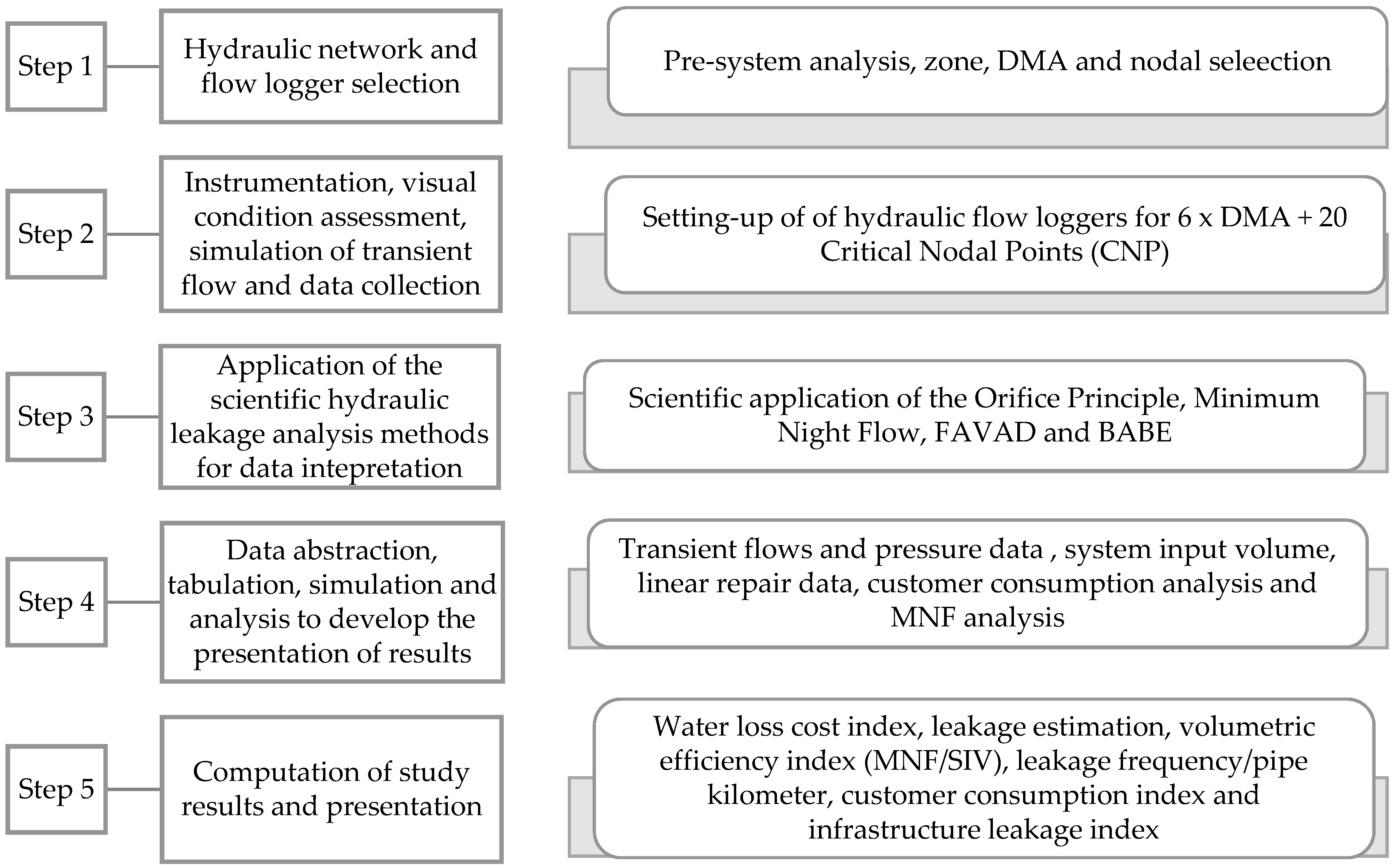
2. Methodology and Materials
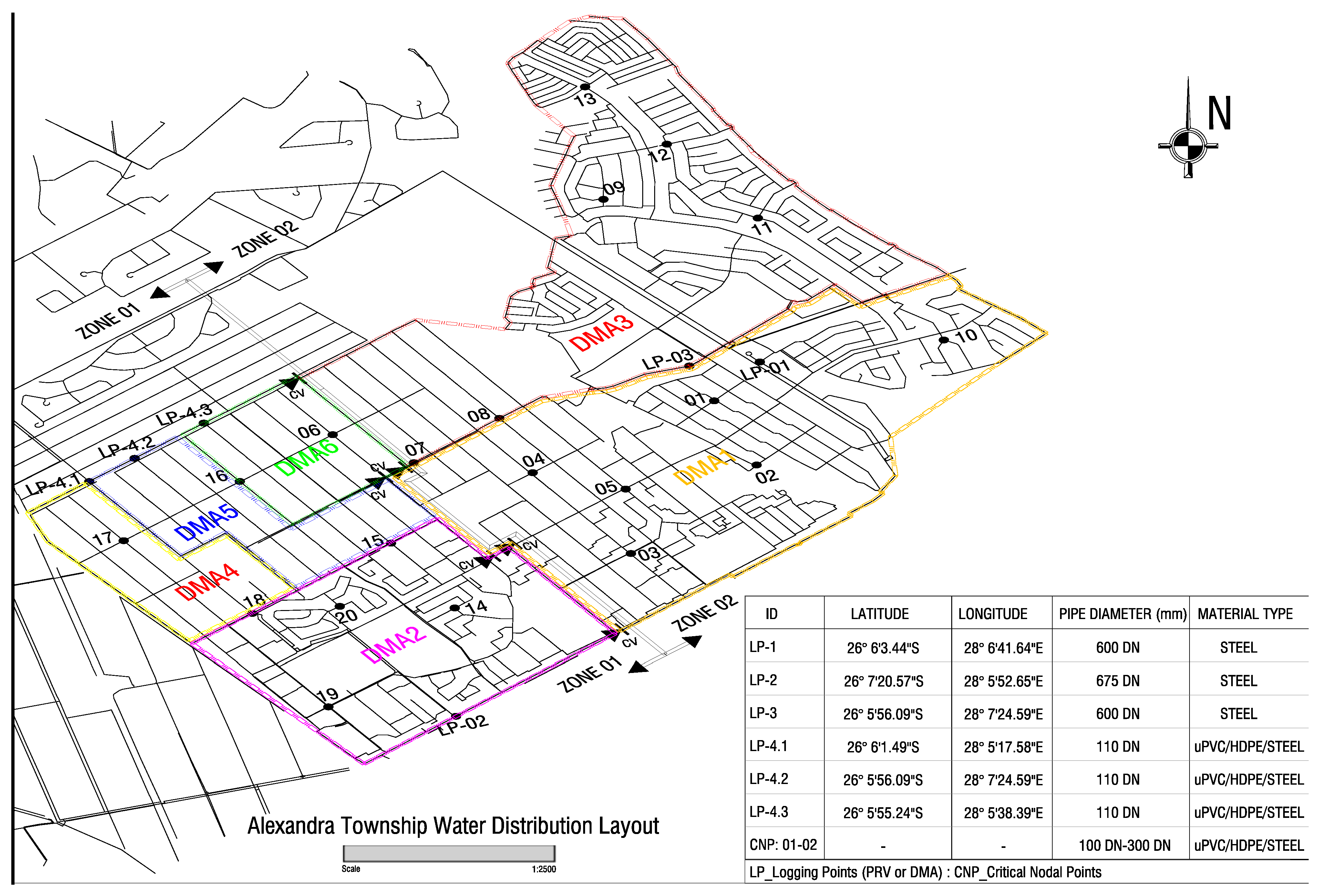
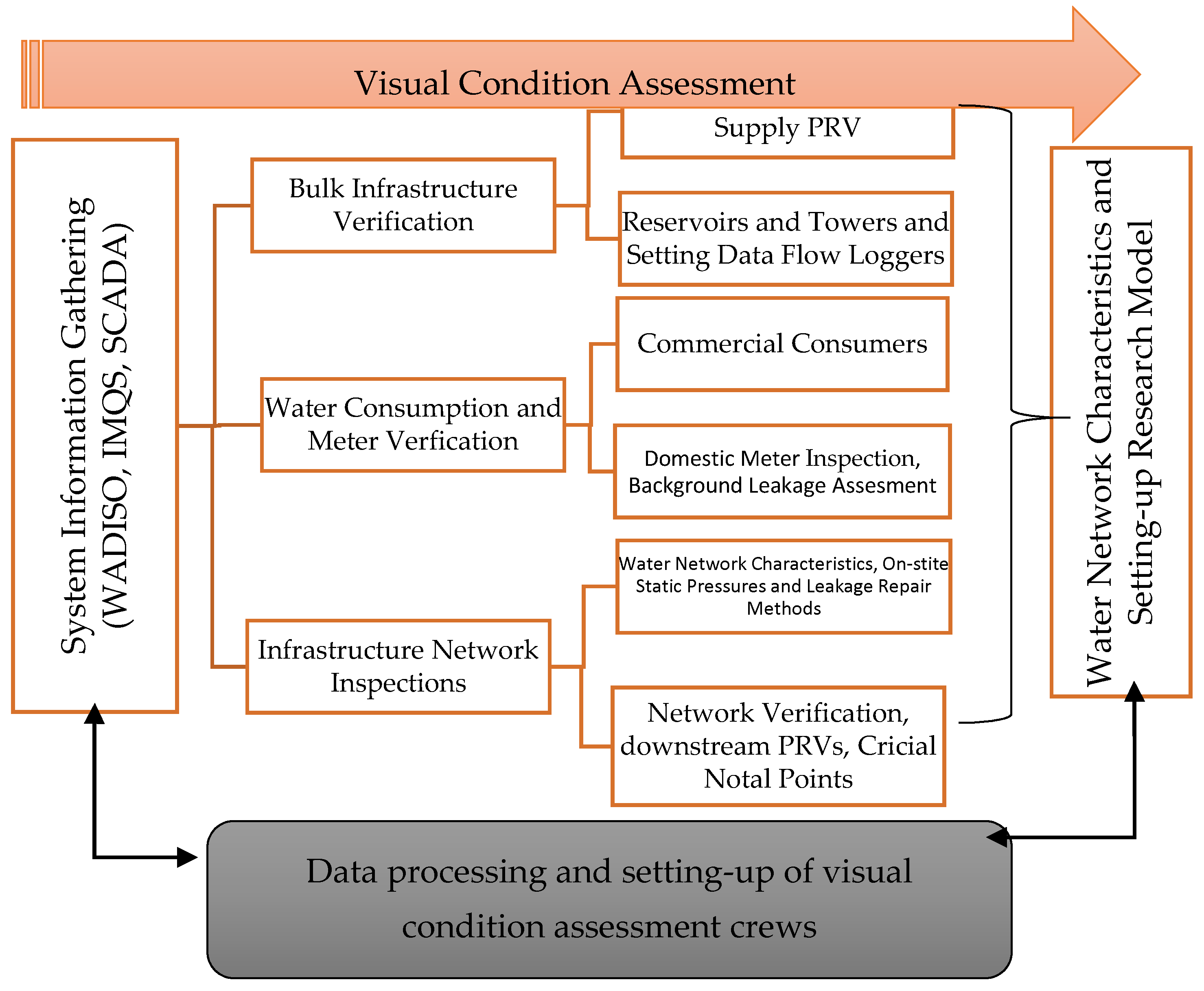
2.1. Preliminary Data Collection and Hydraulic Simulation Process
- a literature search to collect historic loss levels;
- the use of SAP-PM, a customer-centric software application for tracking infrastructure leakage failures, for periods between 2015 and 2019; and
- the use of ultra-sonic flow and pressure logging devices to measure preliminary flow and operating system pressures from the six supplying DMA connections and their flow-modulated PRV.
2.2. Logging and Simulation of the Transient Data Flow and the Indexes’ Computation
2.2.1. Phase 1: Flow and Pressure Simulation Process
2.2.2. Phase 2: Simulation Process
2.2.3. Phase 3: Simulation Process and Computation of Efficiency Indexes
- leakage flowrate ratio;
- leakage frequency/km/pressure linear repair data;
- change in volumetric flow;
- the ratio of MNF/SIV;
- changes in customer consumption; and
- water-saving costs in comparison to the findings of Phase 1.
2.3. Mathematical Formulations
3. Results and Discussion
3.1. Transient Flow Data and Pressure Analysis
3.2. Pressure and Flow Efficiency Index Analysis
3.3. Volumetric Linear Reduction Index
3.4. Leakage Flowrate Results
3.4.1. Linear Repair Results and Indexes
3.4.2. Leakage Estimation
3.4.3. Leakage Cost Indexes
3.4.4. Customer Consumption Index
3.4.5. Infrastructure Leakage Index
4. Conclusions and Recommendations
Author Contributions
Funding
Institutional Review Board Statement
Informed Consent Statement
Data Availability Statement
Acknowledgments
Conflicts of Interest
References
- Chabalala, D.T.; Ndambuki, J.M.; Salim, R.W.; Rwanga, S.S. Impact of climate change on the rainfall pattern of Klip River catchment in Ladysmith, KwaZulu Natal, South Africa. In Proceedings of the 1st International Conference on Sustainable Infrastructural Development, Ota, Nigeria, 24–28 June 2019; IOP Conference Series: Materials Science and Engineering; Covenant University, Registered in England and Wales. IOP Publishing: Bristol, UK, 2019; Volume 640, p. 012088. [Google Scholar] [CrossRef]
- Dighade, R.R.; Kadu, M.S.; Pande, A.M. Challenges in water loss management of water distribution systems in developing countries. Int. J. Innov. Res. Sci. Eng. Technol. 2014, 3, 13838–13846. [Google Scholar]
- Menapace, A.; Zanfei, A.; Felicetti, M.; Avesani, D.; Righetti, M.; Gargano, R. Burst Detection in Water Distribution Systems: The Issue of Dataset Collection. Appl. Sci. 2020, 10, 8219. [Google Scholar] [CrossRef]
- Adedeji, K.B.; Hamam, Y.; Abe, B.T.; Abu-Mahfouz, A.M. Towards Achieving a Reliable Leakage Detection and Localization Algorithm for Application in Water Piping Networks: An Overview. IEEE Access 2017, 5, 20272–20285. [Google Scholar] [CrossRef]
- Chadwick, A.; Morfett, J.; Borthwick, M. Hydraulics in Civil and Environmental Engineering; Spon Press: London, UK, 2001. [Google Scholar] [CrossRef]
- Wu, Z.Y.; Farley, M.; Turtle, D.; Kapelan, Z.; Boxall, J.; Mounce, S.; Dahasahasra, S.; Mulay, M.; Kleiner, Y. Water Loss Reduction; Bentley Institute Press: Exton, PA, USA, 2011. [Google Scholar]
- Darsana, P.; Varija, K. Leakage detection studies for water supply systems—A review. Water Resour. Manag. 2018, 78, 141–150. [Google Scholar]
- Babić, B.; Đukić, A.; Stanić, M. Managing water pressure for water savings in developing countries. Water SA 2014, 40, 221–232. [Google Scholar] [CrossRef] [Green Version]
- Kanakoudis, V.; Tsitsifli, S.; Samaras, P.; Zouboulis, A. Assessing the performance of urban water networks across the EU Mediterranean area: The paradox of high NRW levels and absence of respective reduction measures. Water Sci. Technol. Water Supply 2013, 13, 939–950. [Google Scholar] [CrossRef]
- Thornton, J.; Lambert, A.O. Pressure management extends infrastructure life and reduces unnecessary energy costs. In Proceedings of the IWA International Specialised Conference “Water Loss 2007”, Bucharest, Romania, 23–26 September 2007; pp. 1–9. [Google Scholar]
- Van Zyl, J.E.; Cassa, A.M. Linking the power and FAVAD equations for modeling the effect of pressure on leakage. In Proceedings of the 11th International Computing & Control for the Water Industry Conference, Exeter, UK, 5–7 September 2011; pp. 551–556. [Google Scholar]
- Menapace, A.; Avesani, D. Global Gradient Algorithm Extension to Distributed Pressure Driven Pipe Demand Model. Water Resour. Manag. 2019, 33, 1717–1736. [Google Scholar] [CrossRef] [Green Version]
- Berardi, L.; Laucelli, D.; Ugarelli, R.; Giustolisi, O. Hydraulic system modelling: Background leakage model calibration in Oppegård municipality. Procedia Eng. 2015, 119, 633–642. [Google Scholar] [CrossRef] [Green Version]
- Makaya, E.; Hensel, O. The Contribution of leakage water to total water loss in Harare, Zimbabwe. Int. Res. J. 2014, 3, 55–63. [Google Scholar]
- McKenzie, R.S.; Lambert, A. ECONOLEAK: Economic Model for Leakage Management for Water Suppliers in South Africa, Users Guide; WRC Report TT 169/02; WRC: Pretoria, South Africa, 2002. [Google Scholar]
- Dini, M.; Hemmati, M.; Hashemi, S. Optimal Pump Scheduling to Improve Network Reliability and Leakage in Water Distribution Networks. Water Resour. Manag. 2022, 36, 417–432. [Google Scholar] [CrossRef]
- McKenzie, R.; Siqalaba, Z.N.; Wegelin, W.A. The State of Non-Revenue Water in South Africa; Water Research Commission: Pretoria, South Africa, 2012. [Google Scholar]
- García, I.F.; Novara, D.; Mc Nabola, A. A Model for Selecting the Most Cost-Effective Pressure Control Device for More Sustainable Water Supply Networks. Water 2019, 11, 1297. [Google Scholar] [CrossRef] [Green Version]
- Karadirek, I.E.; Kara, S.; Yilmaz, G.; Muhammetoglu, A. Implementation of hydraulic modeling for water-loss reduction through pressure management. Water Resour. Manag. 2012, 26, 2555–2568. [Google Scholar] [CrossRef]
- Mutikanga, H.E. Water Loss Management: Tools and Methods for Developing Countries. Ph.D. Thesis, Delft University of Technology, Leiden, The Netherlands, 2012. [Google Scholar]
- Trifunovic, N.; Sharma, S.; Pathirana, A. modeling leakage in distribution system using EPANET. In Proceedings of the 5th IWA Water Loss Reduction Specialist Conference, Cape Town, South Africa, 26–30 April 2009; pp. 482–489. [Google Scholar]
- Wegelin, W.A.; McKenzie, R.S.; Siqalaba, Z. Guideline for the Preparation of an IW a Water Balance to Determine Non-Revenue Water and Water Losses; Department of Water and Sanitation: Pretoria, South Africa, 2014. [Google Scholar]
- Martinet, T.; Thetiot, L. Improvement of Belgrade Water Supply System; Final Report; SCE Aménagement-Environnement & Belgrade Water Utility: Belgrade, Serbia, 2006; pp. 62–65. [Google Scholar]
- Babel, M.S.; Islam, S.; Das Gupta, A. Leakage Management in a low-pressure water distribution network of Bangkok. Water Sci. Technol. Water Supply 2009, 9, 141–147. [Google Scholar] [CrossRef]
- Lambert, A.O. International report: Water losses management and techniques. Water Sci. Technol. Water Supply 2002, 2, 1–20. [Google Scholar] [CrossRef] [Green Version]
- Lambert, A.O.; Fantozzi, M. Recent Developments in Pressure Management. In Proceedings of the 6th IWA Water Loss Reduction Specialist Conference, Sao Paulo, Brazil, 6–9 June 2010. [Google Scholar]
- Hashemi, S.S.; Tabesh, M.; Ataeekia, B. Scheduling and operating costs in water distribution networks. Proc. ICE-Water Manag. 2013, 166, 432–442. [Google Scholar] [CrossRef]
- Shirzad, A.; Tabesh, M.; Farmani, R. A comparison between performance of support vector regression and artificial neural network in prediction of pipe burst rate in water distribution networks. KSCE J. Civ. Eng. 2014, 18, 941–948. [Google Scholar] [CrossRef]
- Shirzad, A.; Safari, M.J.S. Pipe failure rate prediction in water distribution networks using multivariate adaptive regression splines and random forest techniques. Urban Water J. 2019, 16, 653. [Google Scholar] [CrossRef]
- Mathye, R.P.; Scholz, M.; Nyende-Byakika, S. Analysis of Domestic Consumption and Background Leakage Trends for Alexandra Township, South Africa. Int. J. Emerg. Technol. 2022, 13, 01–09. [Google Scholar]
- Wilson, M. Participatory Gender-Oriented Information and Learning Needs Assessment of the Youth of Alexandra. Background Report for UNESCO Developing Open Learning Communities for Gender Equity with the Support of ICTs; University of the Witwatersrand: Johannesburg, South Africa, 2002. [Google Scholar]
- World Bank. Local Economic Development: Quick Reference; Urban Development Division, The World Bank: Washington, DC, USA, 2001. [Google Scholar]
- WCWDM. Revised Water Conservation and Water Demand Management Strategy: Internal Report: Johannesburg Water: City of Johannesburg Metropolitan Municipality. WikiWater #227869. 2016. Available online: www.johannesburgwater.co.za (accessed on 15 March 2020).
- Laucelli, D.B.; Meniconi, S. Water distribution network analysis accounting for different background leakage models. Procedia Eng. 2015, 119, 680–689. [Google Scholar] [CrossRef] [Green Version]
- Cassa, A.M.; Van Zyl, J.E.; Laubscher, R.F.; Van Zyl, J. A Numerical Investigation into the Effect of Pressure on Holes and Cracks in Water Supply Pipes. Urban Water J. 2010, 7, 109–120. [Google Scholar] [CrossRef]
- Makaya, E. Water Loss Management Strategies for Developing Countries: Understanding the Dynamics of Water Leakages. Ph.D. Thesis, Universität Kassel/Witzenhausen, Harare, Zimbabwe, 2015. [Google Scholar]
- Thornton, J. Best Management Practice 3: System Water Audits and Leak Detection. Review and Recommendations for Change; Technical Report; California Urban Water Conservation Council, IWA Publishing: London, UK, 2005. [Google Scholar]
- Guo, S.; Zhang, T.-Q.; Shao, W.-Y.; Zhu, D.Z.; Duan, Y.-Y. Two-dimensional pipe leakage through a line crack in water distribution systems. J. Zhejiang Univ. A 2013, 14, 371–376. [Google Scholar] [CrossRef] [Green Version]
- Van Zyl, J.E.; Clayton, C.R.I. The effect of pressure on leakage in water distribution systems. Water Manag. 2007, 160, 109–114. [Google Scholar] [CrossRef]
- van Zyl, J.E.; Haarhoff, J.; Husselmann, M.L. Potential application of end-use demand modelling in South Africa. J. S. Afr. Inst. Civ. Eng. 2003, 45, 9–19. [Google Scholar]
- Massari, C.; Ferrante, M.; Brunone, B.; Meniconi, S. Is the Leak Head–Discharge Relationship in Polyethylene Pipes a Bijective Function? J. Hydraul. Res. 2012, 50, 409–417. [Google Scholar] [CrossRef]
- Lambert, A.O. What do we know about Pressure-Leakage Relationships in Distribution Systems? In Proceedings of the IWA Specialised Conference: System Approach to Leakage Control and Water Distribution Systems Management, Brno, Czech Republic, 16–18 May 2000; pp. 89–96. [Google Scholar]
- Van Zyl, J.E. Theoretical modeling of pressure and leakage in water distribution systems. Procedia Eng. 2014, 89, 273–277. [Google Scholar] [CrossRef] [Green Version]
- Dai, P.D.; Li, P. Optimal pressure regulation in water distribution systems based on an extended model for pressure reducing valves. Water Resour. Manag. 2016, 30, 1239–1254. [Google Scholar] [CrossRef]
- De Marchis, M.; Fontanazza, C.M.; Freni, G.; Notaro, V.; Puleo, V. Experimental Evidence of Leaks in Elastic Pipes. Water Resour. Manag. 2016, 30, 2005–2019. [Google Scholar] [CrossRef]
- Samir, N.; Kansoh, R.; Elbarki, W.; Fleifle, A. Pressure control for minimizing leakage in water distribution systems. Alex. Eng. J. 2017, 56, 601–612. [Google Scholar] [CrossRef]
- Ferrante, M.; Brunone, B.; Meniconi, S.; Capponi, C.; Massari, C. The Leak Law: From Local to Global Scale. Procedia Eng. 2014, 70, 651–659. [Google Scholar] [CrossRef] [Green Version]
- Walker, A. The Independent Review of Charging for Household Water and Sewerage Services. Interim Report; Department for Environment, Food and Rural Affairs: London, UK, 2009. [Google Scholar]
- Ávila, C.; Sánchez-Romero, F.-J.; López-Jiménez, P.; Pérez-Sánchez, M. Leakage Management and Pipe System Efficiency. Its Influence in the Improvement of the Efficiency Indexes. Water 2021, 13, 1909. [Google Scholar] [CrossRef]
- Kanakoudis, V.; Gonelas, K. Applying pressure management to reduce water losses in two Greek cities’ WDSs: Expectations, problems, results, and revisions. Procedia Eng. 2014, 89, 318–325. [Google Scholar] [CrossRef] [Green Version]
- Cavazzini, G.; Pavesi, G.; Ardizzon, G. Optimal assets management of a water distribution network for leakage minimization based on an innovative index. Sustain. Cities Soc. 2000, 54, 101890. [Google Scholar] [CrossRef]
- Fontana, N.; Giugni, M.; Glielmo, L.; Marini, G.; Verrilli, F. Real-time control of a PRV in water distribution networks for pressure regulation: Theoretical framework and laboratory experiments. J. Water Resour. Plan. Manag. 2018, 144, 04017075. [Google Scholar] [CrossRef]
- Girard, M.; Stewart, R.A. Implementation of pressure and leakage management strategies on the Gold Coast, Australia: Case Study. J. Water Resour. Manag. 2007, 133, 210–217. [Google Scholar] [CrossRef] [Green Version]
- Al-Washali, T.; Sharma, S.; Al-Nozaily, F.; Haidera, M.; Kennedy, M. Modelling the Leakage Rate and Reduction Using Minimum Night Flow Analysis in an Intermittent Supply System. Water 2018, 11, 48. [Google Scholar] [CrossRef] [Green Version]
- McKenzie, R.S.; Wegelin, W. Implementation of pressure management in municipal water supply systems. In Proceedings of the EYDAP Conference “Water: The Day After”, Athens, Greece, 6–8 November 2009. [Google Scholar]
- Levin, S.J. An Evaluation of the Pressure-leakage Response of Selected Water Distribution Networks in South Africa. Master’s Thesis, University of Cape Town, Cape Town, South Africa, 2019. [Google Scholar]
- Colombo, A.F.; Karney, B.W. Energy and costs of leaky pipes: Toward comprehensive picture. J. Water Resour. Plan. Manag. 2002, 128, 441–450. [Google Scholar] [CrossRef] [Green Version]
- Marunga, A.; Hoko, Z.; Kaseke, E. Pressure management as a leakage reduction and water demand management tool: The case of the City of Mutare, Zimbabwe. Phys. Chem. Earth 2006, 31, 763–770. [Google Scholar] [CrossRef]
- McKenzie, R. Development of a Standardised Approach to Evaluate Burst and Background Losses in Water Distribution Systems in South Africa; WRC Report TT 109/99; Water Research Commission: Pretoria, South Africa, 1999. [Google Scholar]
- Wegelin, W.A. Guideline for a Robust Assessment of the Potential Savings from Water Conservation and Water Demand Management. Master’s Thesis, Stellenbosch University, Stellenbosch, South Africa, 2015. [Google Scholar]
- Meniconi, S.; Brunone, B.; Ferrante, M.; Mazzetti, E.; Laucelli, D.B.; Borta, G. Transient Effects of Self-adjustment of Pressure Reducing Valves. Procedia Eng. 2015, 119, 1030–1038. [Google Scholar] [CrossRef] [Green Version]


| (a) | |||||||||||
| Name of Reservoir | Elevation | Top Water Level (m) | Static Head (m) | Latitude | Longitude | DMA Supply | Node Supply | ||||
| Linbro Park | 1617.47 | 1642.47 | 100.08 | 26°10′2.90″ S | 28°13′2.89″ S | DMA1, DMA3 | 1, 2, 3, 4, 5, 8, 9, 10, 11, 12, 13 | ||||
| Marlboro | 1592.6 | 1600.12 | 60.00 | 26°09′4.38″ S | 28°08′7.11″ S | DMA4, DMA5, DMA6 | 6,7,15,16,17,18 | ||||
| Randjieslaagte | 1667.64 | 1674.6 | 70.03 | 26°14′1.65″S | 28°09′1.55″S | DMA2 | 14,19,20 | ||||
| (b) | |||||||||||
| Pipeline Details | Average Pressure Outlook | ||||||||||
| ID | PRV Size | Pipe Diameter (mm) | Pipe Material | Pipe Age (Years) | Number of Nodes (DMA) | Energy Grade Line (m) | Elevation (m) | Co-Efficient of Expansion (K-2) | Head (TWL–PRV Elevation) (m) | Total Head (Static + Head Diff) | Dynamic Head (Total Head, EGL–TWL) (m) |
| LP-1 | 300 | 600 | Steel | 22 | +500 | 1596.38 | 1514.74 | 1.2 × 10⁻⁵ | 127.73 | 227.81 | 181.72 |
| LP-2 | 200 | 675 | Steel | 59 | +500 | 1654.79 | 1599.34 | 1.2 × 10⁻⁵ | 75.26 | 145.29 | 125.48 |
| LP-3 | 300 | 600 | Steel | 22 | +500 | 1595.93 | 1523.16 | 1.2 × 10⁻⁵ | 119.31 | 219.39 | 172.85 |
| LP-4.1 | - | 110 | uPVC | 29 | −100 | 1610.26 | 1552.84 | 8 × 10⁻⁵ | 47.28 | 107.28 | 117.42 |
| LP-4.2 | - | 110 | uPVC | 29 | −100 | 1610.27 | 1549.59 | 8 × 10⁻⁵ | 50.53 | 110.53 | 120.68 |
| LP-4.3 | - | 110 | uPVC | 29 | 30–50 | 1610.3 | 1547.82 | 8 × 10⁻⁵ | 52.30 | 112.30 | 122.48 |
| (c) | |||||||||||
| ID | PRV Size | Pipe Diameter (mm) | Pipe Material | Pipe Age (Yrs) | Number of Connection (Node) | Energy Grade Line (m) | Elevation (m) | Co-Efficient of Expansion (K-2) | Head (TWL–PRV Elevation) (m) | Total Head (Static + Head Diff) | Dynamic Head (Total Head, EGL–TWL) (m) |
| 1 | DMA1 | 110 | uPVC | 29 | 4 | 1595.94 | 1515.4 | 8 × 10⁻⁵ | 127.07 | 227.15 | 180.62 |
| 2 | DMA1 | 110 | uPVC | 25 | 3 | 1595.63 | 1554.82 | 8 × 10⁻⁵ | 87.65 | 187.73 | 140.89 |
| 3 | DMA1 | 110 | uPVC | 30 | 4 | 1611.33 | 1547.49 | 8 × 10⁻⁵ | 94.98 | 195.06 | 163.92 |
| 4 | DMA1 | 110 | uPVC | 30 | 4 | 1611.28 | 1544.05 | 8 × 10⁻⁵ | 98.42 | 198.5 | 167.31 |
| 5 | DMA1 | 110 | uPVC | 30 | 4 | 1613.39 | 1550.26 | 8 × 10⁻⁵ | 92.21 | 192.29 | 163.21 |
| 6 | DMA6 | 160 | uPVC | 29 | 4 | 1627.38 | 1594.34 | 8 × 10⁻⁵ | 5.78 | 65.78 | 93.04 |
| 7 | DMA6 | 160 | uPVC | 29 | 4 | 1627.38 | 1520.19 | 8 × 10⁻⁵ | 79.93 | 139.93 | 167.19 |
| 8 | DMA3 | 160 | uPVC | 29 | 3 | 1595.62 | 1520.56 | 8 × 10⁻⁵ | 121.91 | 221.99 | 175.14 |
| 9 | DMA3 | 200 | uPVC | 22 | 3 | 1577.84 | 1541.47 | 8 × 10⁻⁵ | 101 | 201.08 | 136.45 |
| 10 | DMA1 | 100 | steel | 35 | 3 | 1595.27 | 1527.43 | 1.2 × 10⁻⁵ | 115.04 | 215.12 | 167.92 |
| 11 | DMA1 | 110 | uPVC | 23 | 4 | 1570.34 | 1538.59 | 8 × 10⁻⁵ | 103.88 | 203.96 | 131.83 |
| 12 | DMA1 | 110 | uPVC | 25 | 4 | 1568.2 | 1526.95 | 8 × 10⁻⁵ | 115.52 | 215.6 | 141.33 |
| 13 | DMA1 | 110 | HDPE | 10 | 4 | 1562.66 | 1512 | 20 × 10−5 | 130.47 | 230.55 | 150.74 |
| 14 | DMA2 | 100 | steel | 30 | 4 | 1614.75 | 1610.25 | 1.2 × 10⁻⁵ | 64.35 | 134.38 | 74.53 |
| 15 | DMA5 | 300 | uPVC | 30 | 3 | 1595.81 | 1530.99 | 8 × 10⁻⁵ | 111.48 | 211.56 | 164.9 |
| 16 | DMA5 | 110 | uPVC | 29 | 3 | 1610.43 | 1547.62 | 8 × 10⁻⁵ | 94.85 | 194.93 | 162.89 |
| 17 | DMA4 | 110 | uPVC | 29 | 4 | 1659.84 | 1586.96 | 8 × 10⁻⁵ | 55.51 | 155.59 | 172.96 |
| 18 | DMA4 | 100 | HDPE | 18 | 3 | 1610.86 | 1555.88 | 20 × 10−5 | 44.24 | 144.32 | 155.06 |
| 19 | DMA2 | 160 | uPVC | 30 | 4 | 1661.51 | 1600.43 | 8 × 10⁻⁵ | 74.17 | 144.2 | 131.11 |
| 20 | DMA2 | 100 | steel | 30 | 4 | 1613.75 | 1562.5 | 1.2 × 10⁻⁵ | 112.1 | 182.13 | 121.28 |
| Methodology | Mathematical Equation | Research Index Summary Advantages |
|---|---|---|
| Orifice Principle | The method depends on pressure and can be applied in multiple DMAs [34,38,40]. | |
| System Input Volume | This index provides holistic pressure and flow data for the entire water distribution system [14,20,30]. Base data are created for developing a water balance for the DMA, supply zone or an entire bulk system [22]. | |
| Minimum Night Flow | This is the most reliable method for estimating water leakages when consumption is at its lowest in the DMA [6,30,36]. The methodology is beneficial for assessing the effect of variable pressure on leakages during peak and off-peak periods [36]. | |
| Fixed and Variable Area Discharge (FAVAD) | FAVAD integrates the conservation of mass and energy, the orifice principle, the theory of hydraulics of leaks and the effect of variable pressure for leakage estimations [38]. Furthermore, it scientifically caters to turbulent flows due to pressure, material type, the type of leakage and soil hydraulics [35,41]. | |
| Background and Burst Estimate (BABE) | where SIV is the system input volume (m3/month); AC is the authorized consumption (m3/month); and CL is the commercial loss (m3/month) | BABE is beneficial in the bottom-up estimation of system leakages versus customer consumption [14,26,41]. It is a widely used method to measure CARL, ILI and UARL, producing indicative data for the FAVAD principle [6,26,36,42]. |
| Optimal Pressure Management | This index integrates the orifice and FAVAD principle through the simulation of variable pressure before and after the application of pressure management [26,43]. Pressure management is an alternative method for measuring efficiency indexes for water savings, energy savings and leakages per pipe length [40,44,45,46]. | |
| Efficiency Indexes | ||
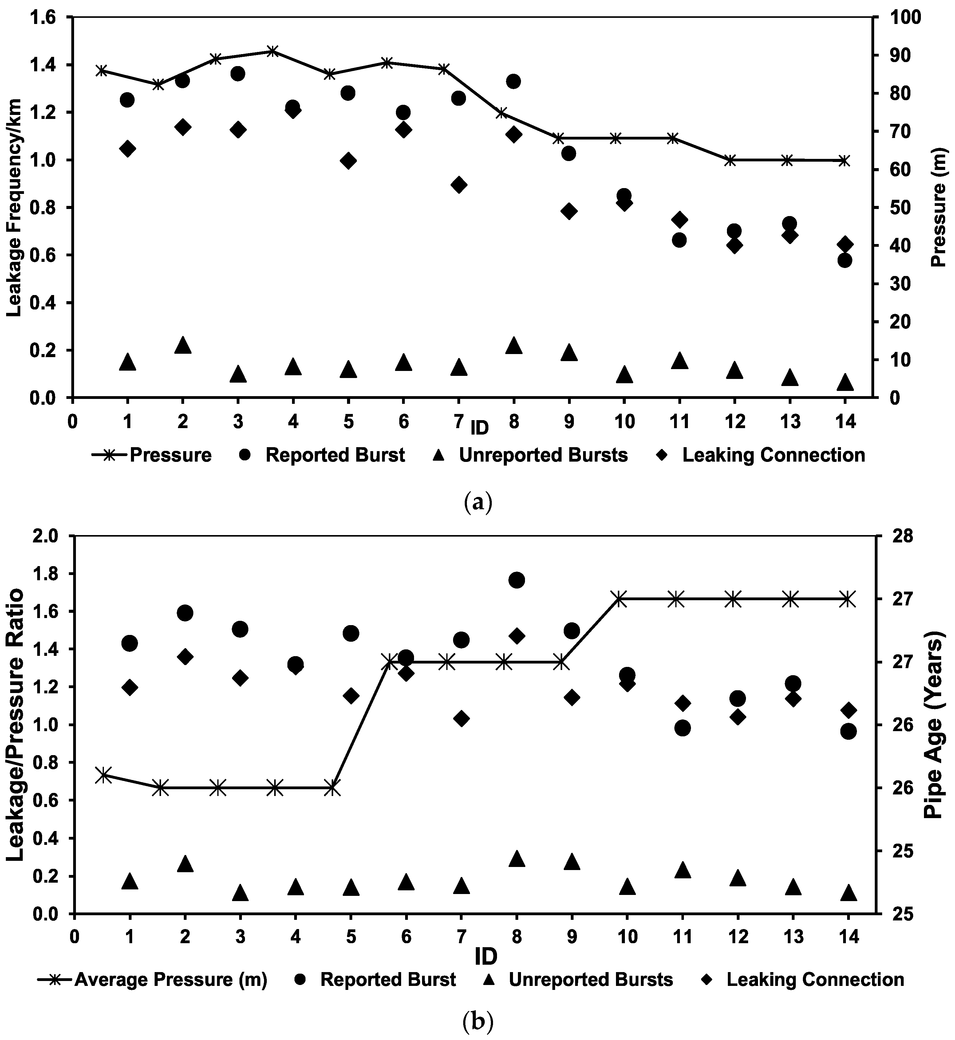
| Leakage Flow Rate | where TLD is the total leakage duration (hour); BS is the basic start date and time when the service ticket was logged on SAP-PM (day or hour); and BF is the basic finish date when a leakage was physically isolated and the repair was initiated (day or hour). where TAVL is the total annual volume of leakage; NRB is the number of reported bursts; ALFR is the average leakage flowrate; and ALD is the average leakage duration | We used the TLD on linear repair abstracted from SAP-PM to set the benchmark for computing TLFR. Leakage durations provide base data for the estimation of real and apparent losses [18]. The method is beneficial when measuring an active leak control (ALC) component in linear leakage repair [14,36,47]. |
| Infrastructure Leakage Index (ILI) | where ILI is the infrastructure leakage index; CARL is the current annual real loss (m3/year); and UARL is the unavoidable annual real loss (m3/year) measured as a component of SIV month by month | According to [17,20], ILI is defined as the ratio of the “current annual real losses” (CARL) to the “unavoidable annual real losses” (UARL). This dimensionless performance indicator was used in this study to assess the comprehensive leakage index in the water distribution system month by month after the reduction in optimum pressure from the PRV. |
| Total Cost of Water | (Note that a unit cost of $3.18/m3 converted from South African Rand/m3 to US Dollar was used in this study) | Water is an economic resource and has a cost value [48]. Therefore, this index provides a base to estimate the cost of water production versus total losses [26]. The authors used this to estimate the total costs of water losses in the water distribution system. |
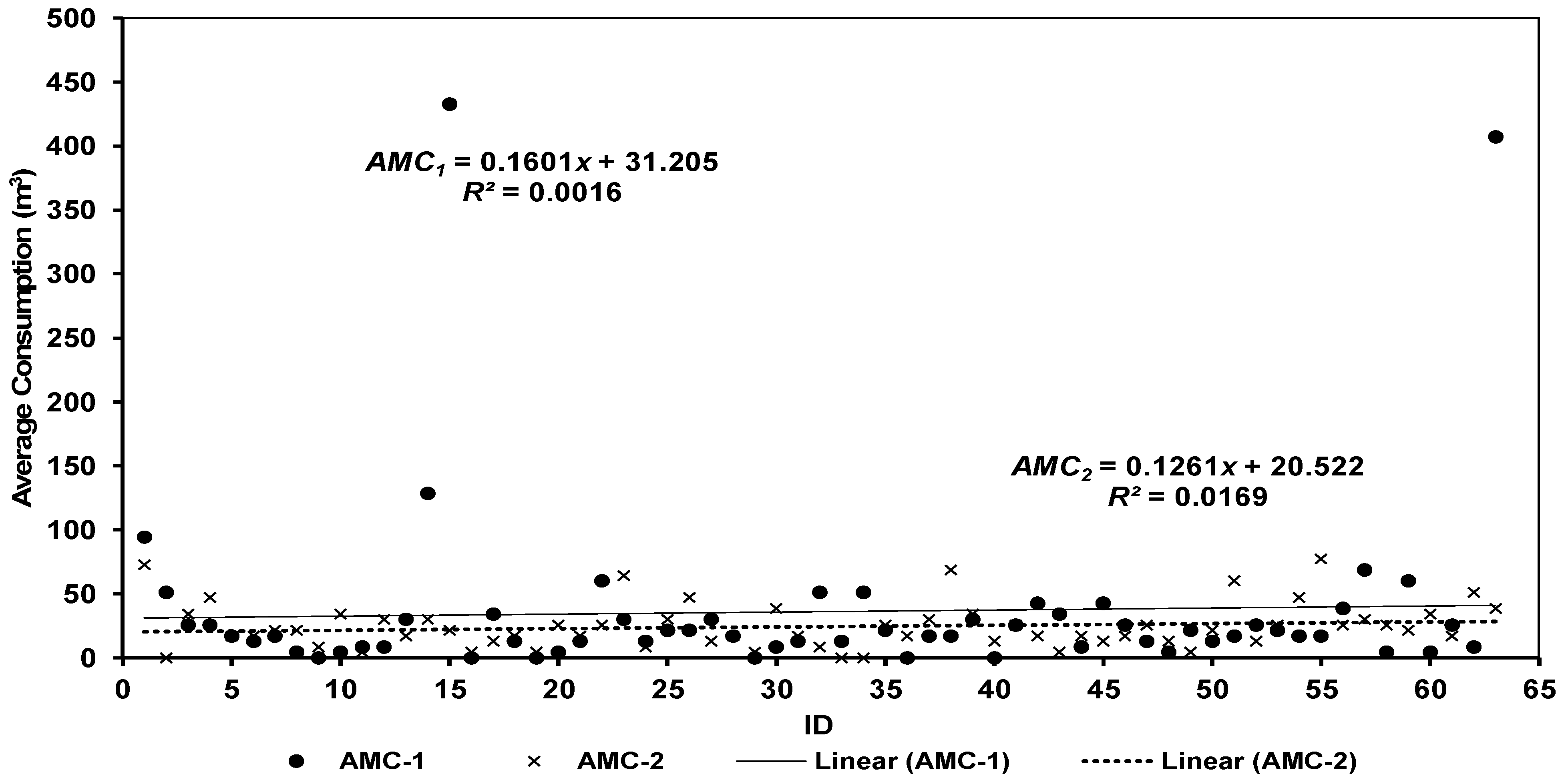
| Customer Consumption Index | where n is the sample size; N is the total number of households; and e is the level of precision at a level of 7 ± 2% | A study by [14] used this index in their study for customer meter consumption assessments. For this study, the authors sampled over 63 properties in the case study area to manually read and record water consumption levels for a period of seven days to establish consumption patterns for Phases 1 and 2. |
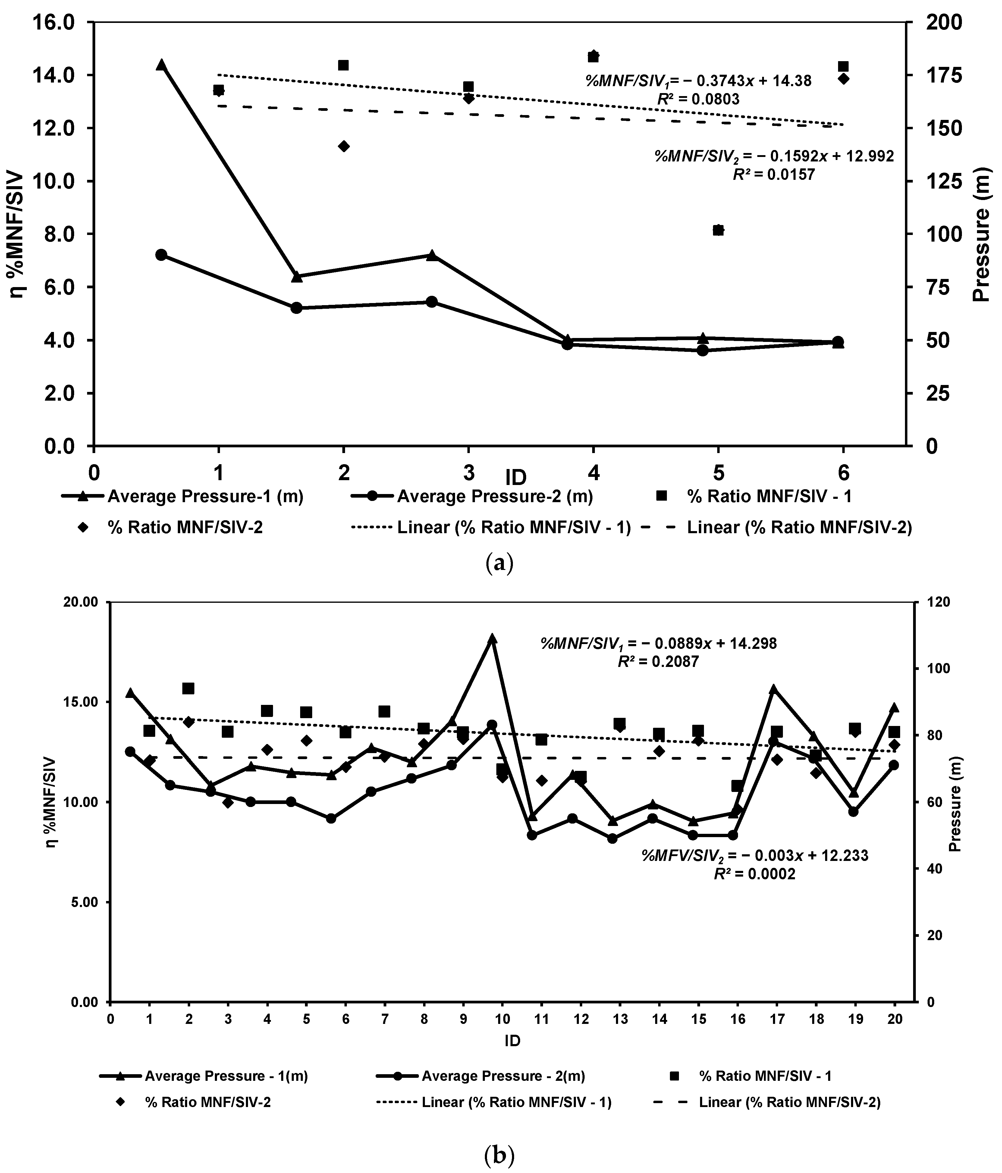
| Pressure Efficiency Index | After resetting downstream operating pressures at each PRV to the required level, the team assessed the following: (1) the percentage change in pressures for Phase 1; and (2) the percentage reduction in MNF/SIV between Phases 1 and 2, as well as the index ratio (IR) of pressure versus %MNF/SIV in Phases 1 and 2. A percentage reduction in these indexes means that a change in optimal pressure has a direct positive impact on leakage control. | |
| Volumetric Efficiency Index | where m is the coefficient value for the linear regression; b is the average constant value of MNF/SIV (l/s); PReduction is the hydraulic system pressure (m); and TLFR is the total leakage flowrate volume as per the reported, unreported and leakage connections. | We used the linear regression analysis method to measure the effect of reduced pressure for the percentage reduction in MNF and SIV by volume. The assessment was carried out at each DMA and 20 critical nodal points (CNPs). Reduction by percentage ratio of MNF/SIV means that a change in optimal pressure is an alternative way to reduce the average flow during off-peak times, e.g., 12:00 a.m. and 4:00 a.m. The authors assessed the percentage index of the total leakages of TLFR/SIV before and after adjusting the PRV to optimal pressures. The reduction in the index ratio means a reduction in infrastructure leakages. |
| Index Ratio for Leakage per Kilometer | The authors further assessed the change in the sum of reported and unreported bursts per kilometer month by month for Phases 1 and 2. They used data abstracted from SAP-PM and IMQS to obtain service failures and the lengths of pipelines. A reduction in the ratio or burst pipe per kilometer indicates a reduction in AZP-reduced bursts and related leakages in water distribution systems and directly translates to water savings. | |
| (a) | ||||||||||||
| Phase 1 | Phase 2 | |||||||||||
| ID | Ave Flow (m3/s) | Ave Pressure (m) | Annual SIV (m3) | Night Flow (m3/s) | Annual MNF (m3) | Ave Flow (m3/s) | Ave Pressure (m) | Annual SIV (m3) | Night Flow (m3/s) | Annual MNF (m3) | Reduced % SIV | Reduced % MNF |
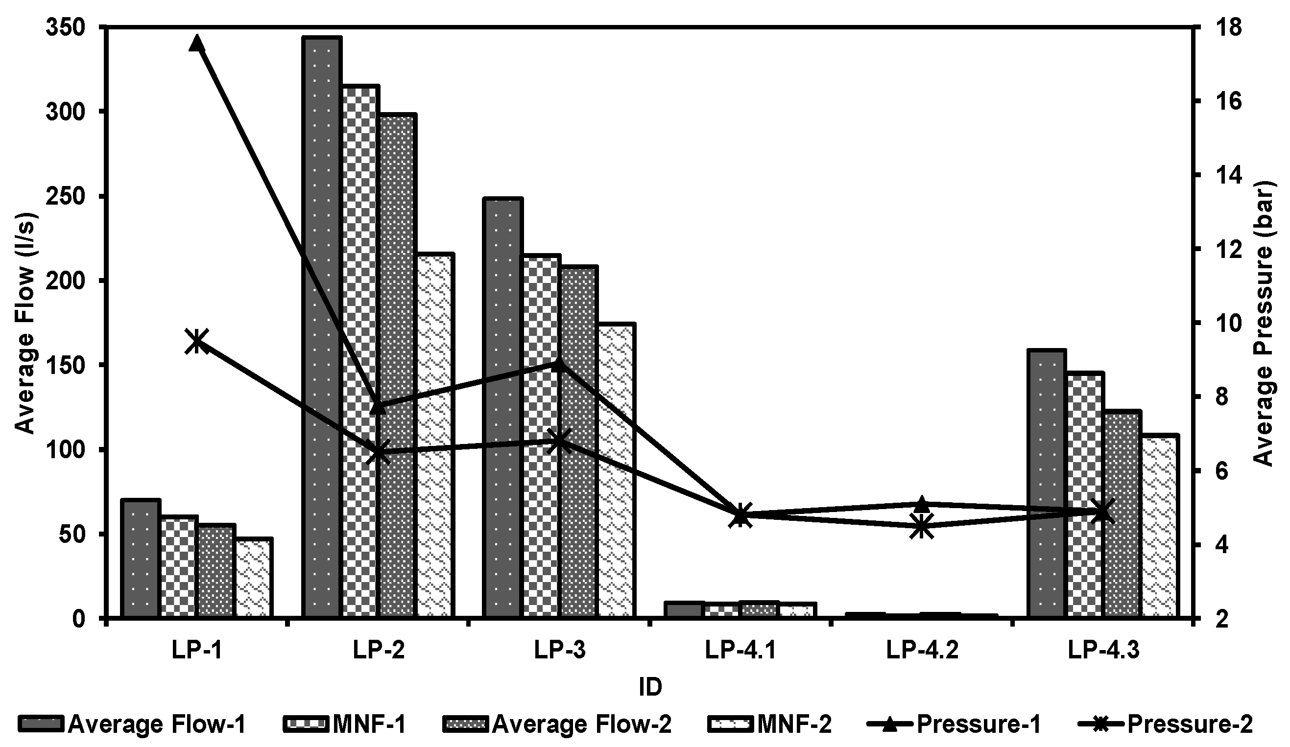
| LP-1 | 70.1 | 180 | 2,209,412 | 60.0 | 296,438 | 55.0 | 90 | 1,734,480 | 47.1 | 232,605 | 21% | 22% |
| LP-2 | 343.8 | 80 | 10,843,338 | 315.0 | 1,556,302 | 298.2 | 65 | 9,404,035 | 215.4 | 1,064,263 | 13% | 32% |
| LP-3 | 248.5 | 90 | 7,836,696 | 215.0 | 1,062,238 | 208.0 | 68 | 6,559,488 | 174.1 | 860,165 | 16% | 19% |
| LP-4.1 | 9.3 | 50 | 293,285 | 8.7 | 42,984 | 8.5 | 48 | 268,056 | 8.0 | 39,525 | 9% | 8% |
| LP-4.2 | 2.7 | 51 | 85,147 | 1.4 | 6917 | 2.7 | 45 | 83,570 | 1.38 | 6818 | 2% | 1% |
| LP-4.3 | 158.7 | 49 | 5,004,700 | 145.0 | 716,393 | 122.6 | 49 | 3,866,314 | 108.5 | 536,059 | 23% | 25% |
| (b) | ||||||||||||
| Phase 1 | Phase 2 | |||||||||||
| ID | Ave Flow (m3/s) | Ave Pressure (m) | Annual SIV (m3) | Night Flow (m3/s) | Annual MNF (m3) | Ave Flow (m3/s) | Ave Pressure (m) | Annual SIV (m3) | Night Flow (m3/s) | Annual MNF (m3) | Reduced % SIV | Reduced % MNF |
| 1 | 0.44 | 92.8 | 13,876 | 0.38 | 1877.4 | 0.35 | 75.0 | 11,038 | 0.27 | 1334.0 | 20% | 29% |
| 2 | 0.31 | 78.9 | 9776 | 0.31 | 1531.6 | 0.28 | 65.0 | 8830 | 0.25 | 1235.2 | 10% | 19% |
| 3 | 0.36 | 65.0 | 11,353 | 0.31 | 1531.6 | 0.33 | 63.0 | 10,407 | 0.21 | 1037.5 | 8% | 32% |
| 4 | 0.42 | 70.7 | 13,245 | 0.39 | 1926.8 | 0.41 | 60.0 | 12,930 | 0.33 | 1630.4 | 2% | 15% |
| 5 | 0.13 | 68.9 | 4100 | 0.12 | 592.9 | 0.12 | 60.0 | 3784 | 0.10 | 494.1 | 8% | 17% |
| 6 | 0.57 | 68.2 | 17,976 | 0.49 | 2420.9 | 0.56 | 55.0 | 17,660 | 0.42 | 2075.1 | 2% | 14% |
| 7 | 0.27 | 76.3 | 8515 | 0.25 | 1235.2 | 0.23 | 63.0 | 7253 | 0.18 | 889.3 | 15% | 28% |
| 8 | 0.39 | 72.0 | 12,299 | 0.34 | 1679.8 | 0.34 | 67.0 | 10,722 | 0.28 | 1383.4 | 13% | 18% |
| 9 | 0.57 | 84.3 | 17,976 | 0.49 | 2420.9 | 0.56 | 71.0 | 17,660 | 0.47 | 2322.1 | 2% | 4% |
| 10 | 0.89 | 109.2 | 28,067 | 0.66 | 3260.8 | 0.39 | 83.0 | 12,299 | 0.28 | 1383.4 | 56% | 58% |
| 11 | 0.61 | 55.9 | 19,237 | 0.51 | 2519.7 | 0.58 | 50.0 | 18,291 | 0.41 | 2025.7 | 5% | 20% |
| 12 | 0.92 | 68.2 | 29,013 | 0.66 | 3260.8 | 0.88 | 55.0 | 27,752 | 0.62 | 3063.2 | 4% | 6% |
| 13 | 0.80 | 54.5 | 25,229 | 0.71 | 3507.9 | 0.65 | 49.0 | 20,498 | 0.57 | 2816.2 | 19% | 20% |
| 14 | 0.11 | 59.4 | 3469 | 0.09 | 464.4 | 0.10 | 55.0 | 3154 | 0.08 | 395.3 | 9% | 15% |
| 15 | 0.22 | 54.3 | 6938 | 0.19 | 938.7 | 0.18 | 50.0 | 5676 | 0.15 | 741.1 | 18% | 21% |
| 16 | 0.45 | 56.7 | 14,191 | 0.31 | 1531.6 | 0.39 | 50.0 | 12,299 | 0.24 | 1185.8 | 13% | 23% |
| 17 | 0.58 | 94.0 | 18,291 | 0.50 | 2470.3 | 0.53 | 78.0 | 16,714 | 0.41 | 2025.7 | 9% | 18% |
| 18 | 0.28 | 79.7 | 8830 | 0.22 | 1086.9 | 0.26 | 73.0 | 8199 | 0.19 | 938.7 | 7% | 14% |
| 19 | 0.62 | 62.9 | 19,552 | 0.54 | 2667.9 | 0.58 | 57.0 | 18,291 | 0.50 | 2470.3 | 6% | 7% |
| 20 | 0.43 | 88.4 | 13,560 | 0.37 | 1828.0 | 0.39 | 71.0 | 12,299 | 0.32 | 1581.0 | 9% | 14% |
| (a) | ||||||||
| Phase 1 | Phase 2 | Efficiency Index | ||||||
| ID | % Ratio MNF/SIV-1 | Average Pressure-1 (m) | % Ratio MNF/SIV-2 | Average Pressure-2 (m) | % Reduction Pressure Ratio (P1–P2) | % Reduction MNF/SIV Ratio (P1–P2) | Index Ratio: Pressure-1/(%MNF/SIV-1) | Index Ratio: Pressure-2/(%MNF/SIV-2) |
| LP-1 | 13.4 | 180 | 13.4 | 90 | 50 | 0.05 | 13.4 | 6.7 |
| LP-2 | 14.4 | 80 | 11.3 | 65 | 19 | 21.15 | 5.6 | 5.7 |
| LP-3 | 13.6 | 90 | 13.1 | 68 | 24 | 3.26 | 6.6 | 5.2 |
| LP-4.1 | 14.7 | 50 | 14.7 | 48 | 4 | −0.61 | 3.4 | 3.3 |
| LP-4.2 | 8.1 | 51 | 8.2 | 45 | 12 | −0.43 | 6.3 | 5.5 |
| LP-4.3 | 14.3 | 49 | 13.9 | 49 | 0 | 3.14 | 3.4 | 3.5 |
| (b) | ||||||||
| Phase 1 | Phase 2 | Efficiency Index | ||||||
| ID | % Ratio MNF/SIV-1 | Average Pressure-1 (m) | % Ratio MNF/SIV-2 | Average Pressure-2 (m) | % Pressure Reduction Ratio (P1–P2) | % Reduction MNF/SIV Ratio (P1–P2) | Index Ratio: Pressure-1/(%MNF/SIV-1) | Index Ratio: Pressure-2/(%MNF/SIV-2) |
| 1 | 13.53 | 93 | 12.1 | 75 | 19 | 11 | 6.86 | 6.21 |
| 2 | 15.67 | 79 | 14.0 | 65 | 18 | 11 | 5.03 | 4.65 |
| 3 | 13.49 | 65 | 10.0 | 63 | 3 | 26 | 4.82 | 6.32 |
| 4 | 14.55 | 71 | 12.6 | 60 | 15 | 13 | 4.86 | 4.76 |
| 5 | 14.46 | 69 | 13.1 | 60 | 13 | 10 | 4.76 | 4.60 |
| 6 | 13.47 | 68 | 11.8 | 55 | 19 | 13 | 5.06 | 4.68 |
| 7 | 14.51 | 76 | 12.3 | 63 | 17 | 15 | 5.26 | 5.14 |
| 8 | 13.66 | 72 | 12.9 | 67 | 7 | 6 | 5.27 | 5.19 |
| 9 | 13.47 | 84 | 13.1 | 71 | 16 | 2 | 6.26 | 5.40 |
| 10 | 11.62 | 109 | 11.2 | 83 | 24 | 3 | 9.40 | 7.38 |
| 11 | 13.10 | 56 | 11.1 | 50 | 10 | 15 | 4.26 | 4.51 |
| 12 | 11.24 | 68 | 11.0 | 55 | 19 | 2 | 6.07 | 4.98 |
| 13 | 13.90 | 54 | 13.7 | 49 | 10 | 1 | 3.92 | 3.57 |
| 14 | 13.39 | 59 | 12.5 | 55 | 7 | 6 | 4.44 | 4.39 |
| 15 | 13.53 | 54 | 13.1 | 50 | 8 | 4 | 4.01 | 3.83 |
| 16 | 10.79 | 57 | 9.6 | 50 | 12 | 11 | 5.25 | 5.19 |
| 17 | 13.51 | 94 | 12.1 | 78 | 17 | 10 | 6.96 | 6.44 |
| 18 | 12.31 | 80 | 11.4 | 73 | 8 | 7 | 6.48 | 6.38 |
| 19 | 13.65 | 63 | 13.5 | 57 | 9 | 1 | 4.61 | 4.22 |
| 20 | 13.48 | 88 | 12.9 | 71 | 20 | 5 | 6.56 | 5.52 |
| Reported Bursts (RBs) | Unreported Bursts (URBs) | Leaking Connection (LC) | Linear Leakage Indexes (LLIs) | |||||||||
|---|---|---|---|---|---|---|---|---|---|---|---|---|
| ID | RB No | ALD (hours) | TAVL (m3) | URB No | ALD (hours) | TAVL (m3) | LC No | ALD (hours) | TAVL (m3) | TLFR (m3) | SIV (m3/month) | TLFR/SIV |
| 1 | 123 | 31.20 | 921,024 | 15 | 73.55 | 132,390 | 103 | 61.01 | 201,089 | 1,254,503 | 2,189,381.50 | 0.57 |
| 2 | 131 | 31.20 | 980,928 | 22 | 73.55 | 194,172 | 112 | 61.01 | 218,660 | 1,393,760 | 2,189,381.50 | 0.64 |
| 3 | 134 | 31.20 | 1,003,392 | 10 | 73.55 | 88,260 | 111 | 61.01 | 216,708 | 1,308,360 | 2,189,381.50 | 0.60 |
| 4 | 120 | 31.20 | 898,560 | 13 | 73.55 | 114,738 | 119 | 61.01 | 232,326 | 1,245,624 | 2,189,381.50 | 0.57 |
| 5 | 126 | 31.20 | 943,488 | 12 | 73.55 | 105,912 | 98 | 61.01 | 191,327 | 1,240,727 | 2,189,381.50 | 0.57 |
| 6 | 119 | 31.20 | 891,072 | 15 | 73.55 | 132,390 | 112 | 61.01 | 218,660 | 1,242,122 | 2,189,381.50 | 0.57 |
| 7 | 125 | 31.20 | 936,000 | 13 | 73.55 | 114,738 | 89 | 61.01 | 173,756 | 1,224,494 | 2,189,381.50 | 0.56 |
| 8 | 132 | 31.20 | 988,416 | 22 | 73.55 | 194,172 | 110 | 61.01 | 214,755 | 1,397,343 | 1,826,328.58 | 0.77 |
| 9 | 102 | 31.20 | 763,776 | 19 | 73.55 | 167,694 | 78 | 61.01 | 152,281 | 1,083,751 | 1,826,328.58 | 0.59 |
| 10 | 86 | 31.20 | 643,968 | 10 | 73.55 | 88,260 | 83 | 61.01 | 162,043 | 894,271 | 1,826,328.58 | 0.49 |
| 11 | 67 | 31.20 | 501,696 | 16 | 73.55 | 141,216 | 76 | 61.01 | 148,376 | 791,288 | 1,826,328.58 | 0.43 |
| 12 | 71 | 31.20 | 531,648 | 12 | 73.55 | 105,912 | 65 | 61.01 | 126,901 | 764,461 | 1,826,328.58 | 0.42 |
| 13 | 76 | 31.20 | 569,088 | 9 | 73.55 | 79,434 | 71 | 61.01 | 138,615 | 787,137 | 1,826,328.58 | 0.43 |
| 14 | 60 | 31.20 | 449,280 | 7 | 73.55 | 61,782 | 67 | 61.01 | 130,805 | 641,867 | 1,826,328.58 | 0.35 |
| Leakage Cost Estimation | % Leakage Cost Index | % MNF Cost Index | % SIV Cost Index | ||||||||
|---|---|---|---|---|---|---|---|---|---|---|---|
| ID | RB | URB | LC | Total Cost | URB | LC | RB | MNF Cost | %MNF | SIV Cost | %SIV |
| 1 | $2,901,226 | $417,029 | $633,430 | $3,951,684 | 6.03% | 0.87% | 1.30% | $966,334 | 8.19% | $6,896,552 | 7.79% |
| 2 | $3,089,923 | $611,642 | $688,779 | $4,390,344 | 6.42% | 1.27% | 1.40% | $966,334 | 8.19% | $6,896,552 | 7.79% |
| 3 | $3,160,685 | $278,019 | $682,629 | $4,121,332 | 6.57% | 0.58% | 1.40% | $966,334 | 8.19% | $6,896,552 | 7.79% |
| 4 | $2,830,464 | $361,425 | $731,827 | $3,923,716 | 5.88% | 0.75% | 1.50% | $966,334 | 8.19% | $6,896,552 | 7.79% |
| 5 | $2,971,987 | $333,623 | $602,681 | $3,908,291 | 6.18% | 0.69% | 1.30% | $966,334 | 8.19% | $6,896,552 | 7.79% |
| 6 | $2,806,877 | $417,029 | $688,779 | $3,912,684 | 5.84% | 0.87% | 1.40% | $966,334 | 8.19% | $6,896,552 | 7.79% |
| 7 | $2,948,400 | $361,425 | $547,333 | $3,857,158 | 6.13% | 0.75% | 1.10% | $966,334 | 8.19% | $6,896,552 | 7.79% |
| 8 | $3,113,510 | $611,642 | $676,479 | $4,401,631 | 6.47% | 1.27% | 1.40% | $719,102 | 6.10% | $5,752,935 | 6.50% |
| 9 | $2,405,894 | $528,236 | $479,685 | $3,413,816 | 5.00% | 1.10% | 1.00% | $719,102 | 6.10% | $5,752,935 | 6.50% |
| 10 | $2,028,499 | $278,019 | $510,434 | $2,816,952 | 4.22% | 0.58% | 1.10% | $719,102 | 6.10% | $5,752,935 | 6.50% |
| 11 | $1,580,342 | $444,830 | $467,385 | $2,492,558 | 3.29% | 0.92% | 1.00% | $719,102 | 6.10% | $5,752,935 | 6.50% |
| 12 | $1,674,691 | $333,623 | $399,738 | $2,408,052 | 3.48% | 0.69% | 0.80% | $719,102 | 6.10% | $5,752,935 | 6.50% |
| 13 | $1,792,627 | $250,217 | $436,636 | $2,479,481 | 3.73% | 0.52% | 0.90% | $719,102 | 6.10% | $5,752,935 | 6.50% |
| 14 | $1,415,232 | $194,613 | $412,037 | $2,021,882 | 2.94% | 0.40% | 0.90% | $719,102 | 6.10% | $5,752,935 | 6.50% |
| ID | SIV | AMC | AC | CL | CARL | L (km) | N (c) | L (p) | P (AVE) | UARL | ILI |
|---|---|---|---|---|---|---|---|---|---|---|---|
| 1 | 2,189,381 | 36.33 | 178,807 | 0 | 2,010,574 | 98,435 | 4922 | 0 | 86.0 | 490,994 | 4.1 |
| 2 | 2,189,381 | 36.33 | 178,807 | 0 | 2,010,574 | 98,435 | 4922 | 0 | 82.3 | 469,870 | 4.3 |
| 3 | 2,189,381 | 36.33 | 178,807 | 0 | 2,010,574 | 98,435 | 4922 | 0 | 89.0 | 508,122 | 4.0 |
| 4 | 2,189,381 | 36.33 | 178,807 | 0 | 2,010,574 | 98,435 | 4922 | 0 | 91.0 | 519,540 | 3.9 |
| 5 | 2,189,381 | 36.33 | 178,807 | 0 | 2,010,574 | 98,435 | 4922 | 0 | 85.0 | 485,285 | 4.1 |
| 6 | 2,189,381 | 36.33 | 180,547 | 0 | 2,008,834 | 99,393 | 4970 | 0 | 88.0 | 507,302 | 4.0 |
| 7 | 2,189,381 | 36.33 | 180,547 | 0 | 2,008,834 | 99,393 | 4970 | 0 | 86.3 | 497,502 | 4.0 |
| 8 | 1,826,329 | 36.33 | 180,547 | 0 | 1,645,781 | 99,393 | 4970 | 0 | 74.8 | 431,207 | 3.8 |
| 9 | 1,826,329 | 24.56 | 122,055 | 0 | 1,704,274 | 99,393 | 4970 | 0 | 68.2 | 393,159 | 4.3 |
| 10 | 1,826,329 | 24.56 | 124,593 | 0 | 1,701,736 | 101,460 | 5073 | 0 | 68.2 | 401,335 | 4.2 |
| 11 | 1,826,329 | 24.56 | 124,593 | 0 | 1,701,736 | 101,460 | 5073 | 0 | 68.2 | 401,335 | 4.2 |
| 12 | 1,826,329 | 24.56 | 124,593 | 0 | 1,701,736 | 101,460 | 5073 | 0 | 62.4 | 367,204 | 4.6 |
| 13 | 1,826,329 | 24.56 | 127,723 | 0 | 1,698,606 | 104,009 | 5200 | 0 | 62.4 | 376,429 | 4.5 |
| 14 | 1,826,329 | 24.56 | 127,723 | 0 | 1,698,607 | 104,009 | 5200 | 0 | 62.3 | 375,826 | 4.5 |
Publisher’s Note: MDPI stays neutral with regard to jurisdictional claims in published maps and institutional affiliations. |
© 2022 by the authors. Licensee MDPI, Basel, Switzerland. This article is an open access article distributed under the terms and conditions of the Creative Commons Attribution (CC BY) license (https://creativecommons.org/licenses/by/4.0/).
Share and Cite
Mathye, R.P.; Scholz, M.; Nyende-Byakika, S. Optimal Pressure Management in Water Distribution Systems: Efficiency Indexes for Volumetric Cost Performance, Consumption and Linear Leakage Measurements. Water 2022, 14, 805. https://doi.org/10.3390/w14050805
Mathye RP, Scholz M, Nyende-Byakika S. Optimal Pressure Management in Water Distribution Systems: Efficiency Indexes for Volumetric Cost Performance, Consumption and Linear Leakage Measurements. Water. 2022; 14(5):805. https://doi.org/10.3390/w14050805
Chicago/Turabian StyleMathye, Risimati Patrick, Miklas Scholz, and Stephen Nyende-Byakika. 2022. "Optimal Pressure Management in Water Distribution Systems: Efficiency Indexes for Volumetric Cost Performance, Consumption and Linear Leakage Measurements" Water 14, no. 5: 805. https://doi.org/10.3390/w14050805