Spatial and Temporal Patterns of Low-Flow Changes in Lowland Rivers

Abstract

At the beginning of the 21st century, ongoing climate change led to research into extreme streamflow phenomena. This study aimed to assess the patterns of low-flow changes in different hydrological regions of Lithuania using selected hydrological indices (the annual minimum 30-day flow (m³ s⁻¹) of the warm period—30Q), its duration, and deficit volume (below the 80th and 95th percentile flow: 30Q80 and 30Q95). Differences in low-flow indices in separate hydrological regions and over different periods (1961–2020, 1961–1990, 1991–2020) were analyzed, applying the HydroOffice tool, the TREND software package, and mapping using the Kriging interpolation. The highest specific indices of 30Q were estimated in the Southeastern hydrological region (3.97 L/s·km²) and the lowest in the Central hydrological region (1.47 L/s·km²). In general, the 30Q values in the periods 1961–2020 and 1991–2020 had no trends. In 1961–1990, trends in 30Q data were significantly positive, and positive in most investigated rivers of the Western and Central hydrological regions. The average number of dry days at both thresholds decreased in the Western and Southeastern hydrological regions and increased in the Central hydrological region comparing two subperiods.

1. Introduction

Low flow is a seasonal phenomenon and a basic component of the river flow regime [1]. Low flows occur after periods of low rainfall or when precipitation falls as snow [2]. Since one or both situations occur annually in many regions, by the season of occurrence, low flows are described as summer low flow and winter low flow. Low flow is a compulsory component in the ecological integrity of most river systems; low-flow timing and duration are critical features regarding aquatic ecosystem viability, as well as sufficient water quality and supply [3]. Under extreme and prolonged low-flow conditions, instream habitats are reduced, become fragmented or lost, aquatic species lack the ability to disperse due to the altered environment, alteration of food resources occurs, changes in the strength and structure of interspecific interactions are observed, etc. [4,5,6,7]. Water scarcity threatens the ecosystem, businesses, and the community. The Communication on Water Scarcity and Drought [8], adopted by the European Commission in 2007, highlights the emerging challenge of basic needs so that every human being and most economic activities have access to sufficient good quality water. A recent report of IPCC [9] warns of a continuing rise in global surface temperature until at least the mid-century, with all emissions scenarios considered. As a result, the seasonal flow regime of the river is going to experience significant alterations through a variety of (potentially interfering) mechanisms, including shifts in the temporal and spatial precipitation pattern, changes in snow-melt timing due to rising temperature, or increasing evaporation demand [10,11,12].

Low-flow patterns depend on geographical, climatic, and anthropogenic factors [13]. A study of seasonal timing and the main drivers of low flows across 1860 European and US catchments [13] revealed that low flows tend to occur in either late summer/autumn or winter across these study regions. In Europe, winter low flows occur mainly in the Alps and northern Scandinavia; in the rest of the European sites, annual low flows are observed almost exclusively in late summer (August and September) and are primarily associated with periods of high excess potential evapotranspiration. The records of near-natural streamflow from 441 small catchments in 15 countries across Europe showed that low flows have increased in most winter low-flow regimes and decreased in most summer low-flow regimes [10]. However, on a finer scale, the authors found that decreasing trends are often weak in the areas with summer low-flow regimes and patterns of directionality are mixed; positive trends predominate around the Baltic Sea and are found locally elsewhere. A study based on thousands of time series of river flows and hydrological extremes across the globe [14] found that the observed trends can only be explained if the effects of climate change are considered.

To describe and analyze low-flow regimes, researchers often use a variety of hydrological indices, such as mean minimum monthly flows, low-flow index, low-flow pulse count and duration, annual minima of 1-/3-/7-/30-/90-day means of daily discharge, low exceedance flows, etc. [15]. Since maintaining a certain low flow in a river is related to defining environmental flow standards, such indices are widely used and, in some countries, are officially adopted. Trends in low flows of German rivers were analyzed using annual minimum low flows (for 1-/7-/14-/21-/30-/60-/90-days), discharge deficits (below Q90 and Q95 by calendar year), and low-flow durations (below Q90 and Q95 by calendar year) [16]. Although each index is applied for different purposes in water management applications, the authors found similar spatial patterns for all used indices. The study of trend detection in river flow indices [17] stated that, in Poland, in general, decreases of low flow, expressed as the annual minima of 7-day averaged daily flows, were observed in areas where the mean river flow was low. The applied mean summer minimum discharge did not indicate an expected significant decrease in low flows in the most studied Central European headwaters [18]. In contrast, results based on the 7-day annual minimum streamflow and the 10th percentile of the annual flow duration curve showed a general decline in low flows throughout the rivers in Spain [19]. In Ireland, statistically significant trends in the 7-day sustained low-flow time series of mixed direction were identified only at a part of studied gauging stations [20]. No clearly pronounced decrease in low flows was detected using annual minimum 30-day flow (m³ s⁻¹) and prevalence of low flows (number of days below the 90th percentile flow) based on 120 near-natural catchments in the UK [21]. Statistical analysis of average low flow and minimum monthly summer and winter discharges showed significant positive trends in all parameters of the low-water period in the rivers of the European part of Russia [22]. Analysis of the Latvian river discharge regime revealed that, in most cases, there were no statistically significant overall long-term changes in low-flow discharges of the warm period (defined as a series of the 30-day minimum discharge in May–October); however, a statistically significant upward trend in low flow during the cold period was found [23].

In Lithuania, low flows typically occur during extended dry periods in the late summer and early autumn. For many years, only a limited number of studies have been related to this critical component of a river flow regime. However, at the beginning of the 21st century, research into extreme streamflow phenomena has intensified with the growing evidence of climate change. Low-flow changes in Lithuanian rivers in the 20th century (more precisely—till 2003) were investigated [24]. The authors identified the cyclic variations in the 30-day minimum discharge series, but no significant trends of this characteristic were detected. The meteorological and hydrological drought patterns were analyzed in the Lithuanian permanent rivers [25]. It has been established that climate change predicted at the end of the 21st century may increase the likelihood of more intense and frequent meteorological droughts in Lithuania [26]. Summer flows projections in the studied rivers showed a decreasing tendency [27,28]. The ongoing signs of climate change led to the investigation of intermittent rivers, which are particularly sensitive to any alterations in meteorological conditions or any anthropogenic disturbances [29].

Although the summer low-flow period is a critical time for water users and aquatic ecosystems, the spatial and temporal behavior of low flows in Lithuanian catchments is not fully understood. This study, therefore, set out to assess the patterns of low-flow changes in different hydrological regions of Lithuania using selected hydrological indices. The paper analyzed the annual minimum 30-day flow (m³ s⁻¹) of the warm period (30Q), its duration, and deficit volume (below the 80th and 95th percentile flow: 30Q80 and 30Q95). The defined differences in low-flow indices in different hydrological regions and over different periods (1961–2020, 1961–1990, 1991–2020) provide a better understanding of low-flow behavior in lowland river catchments.

2. Materials and Methods

2.1. Study Area and Data

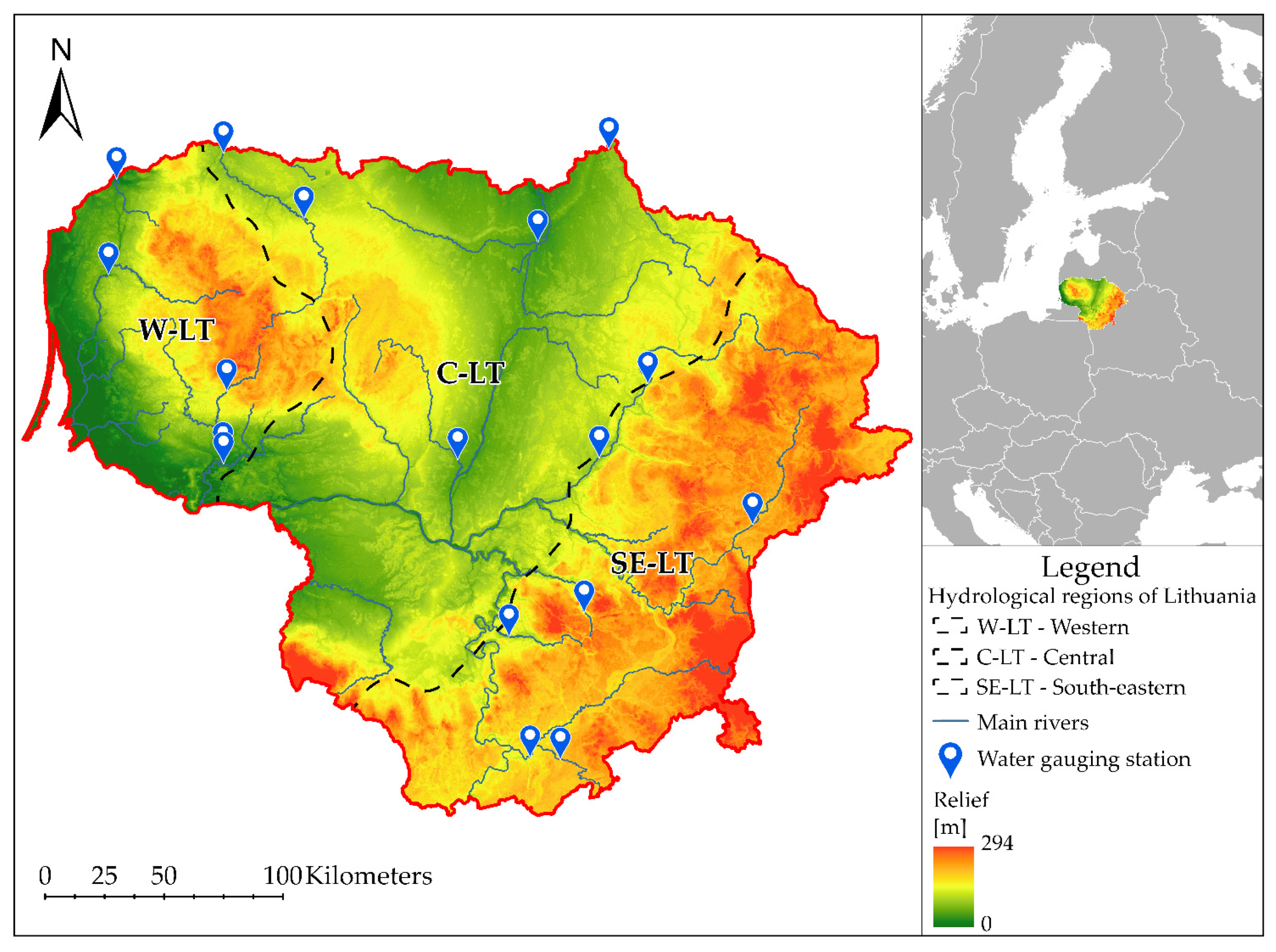
Lithuania (total area of 65,200 km²) has over 22,000 rivers with a total length exceeding 37,000 km. The annual river runoff varies from 4.2 to 14.0 L/(s·km²). The Nemunas River is a major Lithuanian river. Its total length is 937 km, while the basin area covers 98,200 km², of which 46,600 km² belong to Lithuania (comprising 72% of Lithuanian territory). Climatic factors, soil structure, geology, geomorphology, and anthropogenic activities affect the hydrological regime of the Lithuanian rivers [29]. According to the hydrological regime and the river feeding type, the territory of Lithuania is divided into three hydrological regions (Figure 1): Western (W-LT), Central (C-LT), and Southeastern (SE-LT). In the W-LT region, the main source of river feeding is precipitation. In the SE-LT region, subsurface feeding dominates: widespread permeable sandy soils effectively absorb snowmelt water and gradually release it later, supplying rivers during the low-water period. The type of river feeding in the C-LT region is mixed; the rivers here obtain water mostly from two main sources: rainfall and snowmelt. Very irregular distribution of discharges throughout the year is the main feature of the rivers in this region.

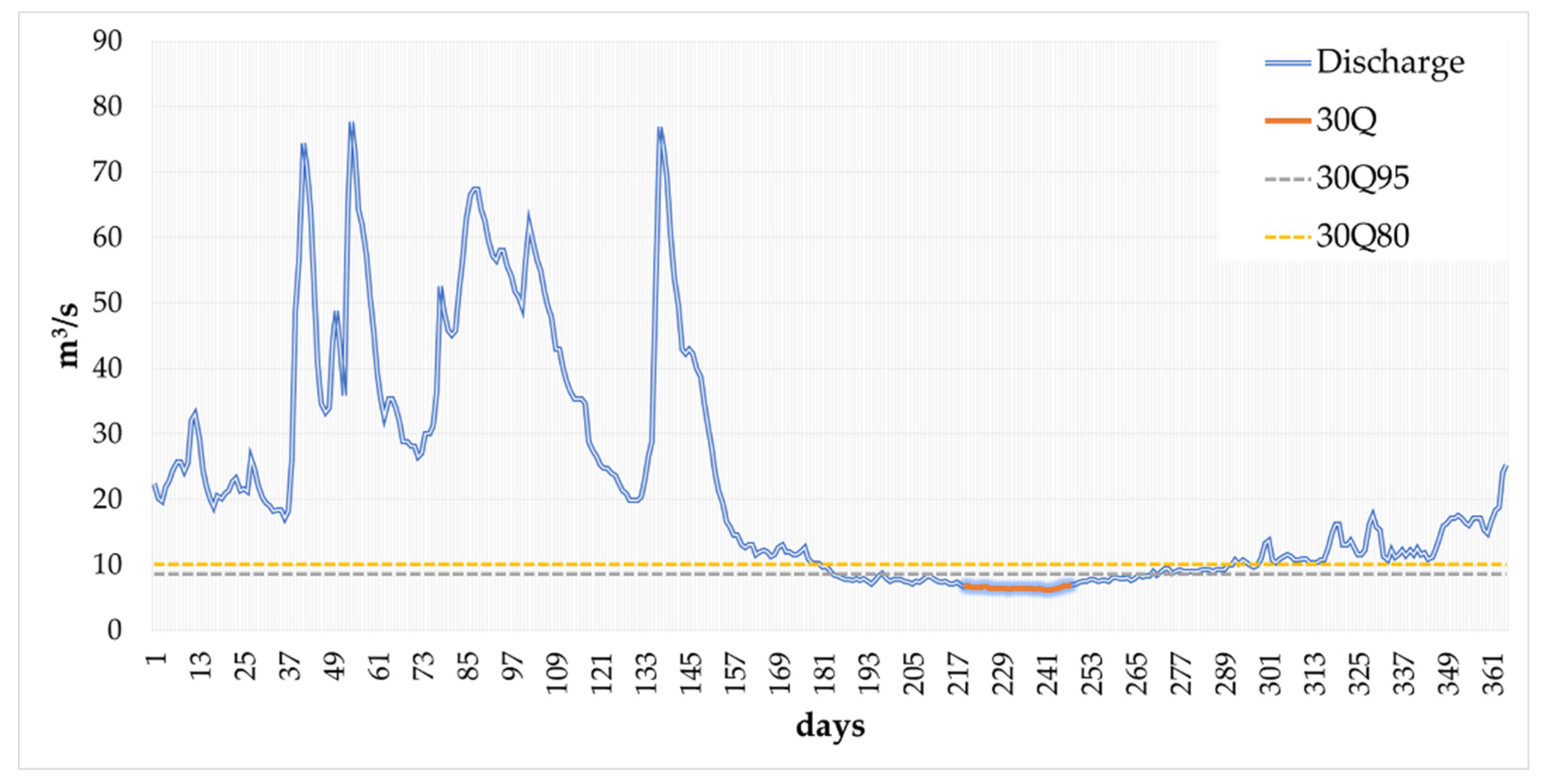
Daily discharge data (1961–2020) from 17 water gauging stations (WGS) in different hydrological regions were used for this study (

Table 1. Characteristics of selected water gauging stations (1961–2020).

№	River	WGS	Abbreviation	A, km2	Qav, m3/s	30Qav, m3/s	30Q95, m3/s	30Q80, m3/s
Western hydrological region
1.	Jūra	Tauragė	JUR	1690	22.05	3.72	1.62	2.43
2.	Akmena	Paakmenis	AKM	314	4.29	0.69	0.30	0.45
3.	Minija	Kartena	MIN	1230	16.56	2.93	1.32	1.77
4.	Bartuva	Skuodas	BAR	612	7.55	0.76	0.30	0.50
Central hydrological region
5.	Šušvė	Josvainiai	SUS	1100	5.62	0.62	0.22	0.33
6.	Šešuvis	Skirgailai	SES	1880	15.20	2.47	1.19	1.72
7.	Nemunėlis	Tabokinė	NEM	2690	19.63	3.12	1.19	1.81
8.	Mūša	Ustukiai	MUS	2280	10.40	1.37	0.53	0.70
9.	Venta	Papilė	VEN1	1570	9.81	1.67	0.73	1.08
10.	Venta	Leckava	VEN2	4060	29.91	5.24	2.32	3.10
Southeastern hydrological region
11.	Merkys	Puvočiai	MER	4300	31.92	21.79	16.20	18.43
12.	Ūla	Zervynos	ULA	679	4.88	2.93	1.94	2.42
13.	Verknė	Verbyliškės	VER	694	5.05	2.16	1.46	1.78
14.	Strėva	Semeliškės	STR	234	1.65	1.00	0.69	0.82
15.	Žeimena	Pabradė	ZEI	2580	20.46	12.14	8.09	10.15
16.	Šventoji	Anykščiai	SVE1	3600	26.46	10.32	3.96	7.41
17.	Šventoji	Ukmergė	SVE2	5440	39.05	14.51	6.48	10.05

). These data sets were obtained from the Lithuanian Hydrometeorological Service. In this study, low flows were defined as the 30-day minimum discharge (30Q, m³/s) and were calculated for each year (average of 30Q in the period 1961–2020 was defined from 30Q_av); this definition in Lithuanian hydrology was formed historically due to the frequent violation of low flow stability by rain floods in summer. Thus, 30Q is less prone to critical deviations that show values over a shorter period (e.g., 1, 3, 5, 7 days) and eliminates deviations caused by precipitation. The 30Q95 and 30Q80 flow quantiles were estimated from the 30Q time series. The homogeneity of used daily discharge data for 1961–2002 was checked by the Standard Normal Homogeneity Test (SNHT) and the Pettitt Test.

2.2. Methods

There are two types of low flows in Lithuania—winter and summer–autumn. This study focused on the summer low-flow events observed from 1 May to 31 October. A typical hydrograph of a river in the SE-LT region and selected low-flow indices are presented in Figure 2.

Low flows were calculated for the periods of 1961–2020, 1961–1990, and 1991–2020. Generally, in Lithuanian catchments, the period of 30Q is observed in summer and autumn, and it differs depending on the hydrological region. In addition, two more indices of low flow were estimated: 30Q95 and 30Q80. For calculation of mentioned indices, the data set of 30Q, which was equal to or exceeding 95% and 80% of all values, was used. These indices were used as a threshold for estimating the duration of low flow and deficit volume. To facilitate the comparison of the low-flow indices on various spatial scales, a specific low-flow q (30q, 30q95, and 30q80) was calculated, which should be defined as q = Q/A·1000 (where Q is 30Q/30Q95/30Q80 low flow discharge in m³/s, A—the catchment area in km²). Modular coefficients for the low-flow period K = 30Q_i/30Q_av (30Q_i is the discharge in year i, and 30Q_av is the average discharge for the entire period of observation) were used to estimate the regularities and to examine how low flows differed by decades (1961–2020) in the rivers from the different hydrological regions. This relative coefficient K enables a comparison of the rivers with different runoff values.

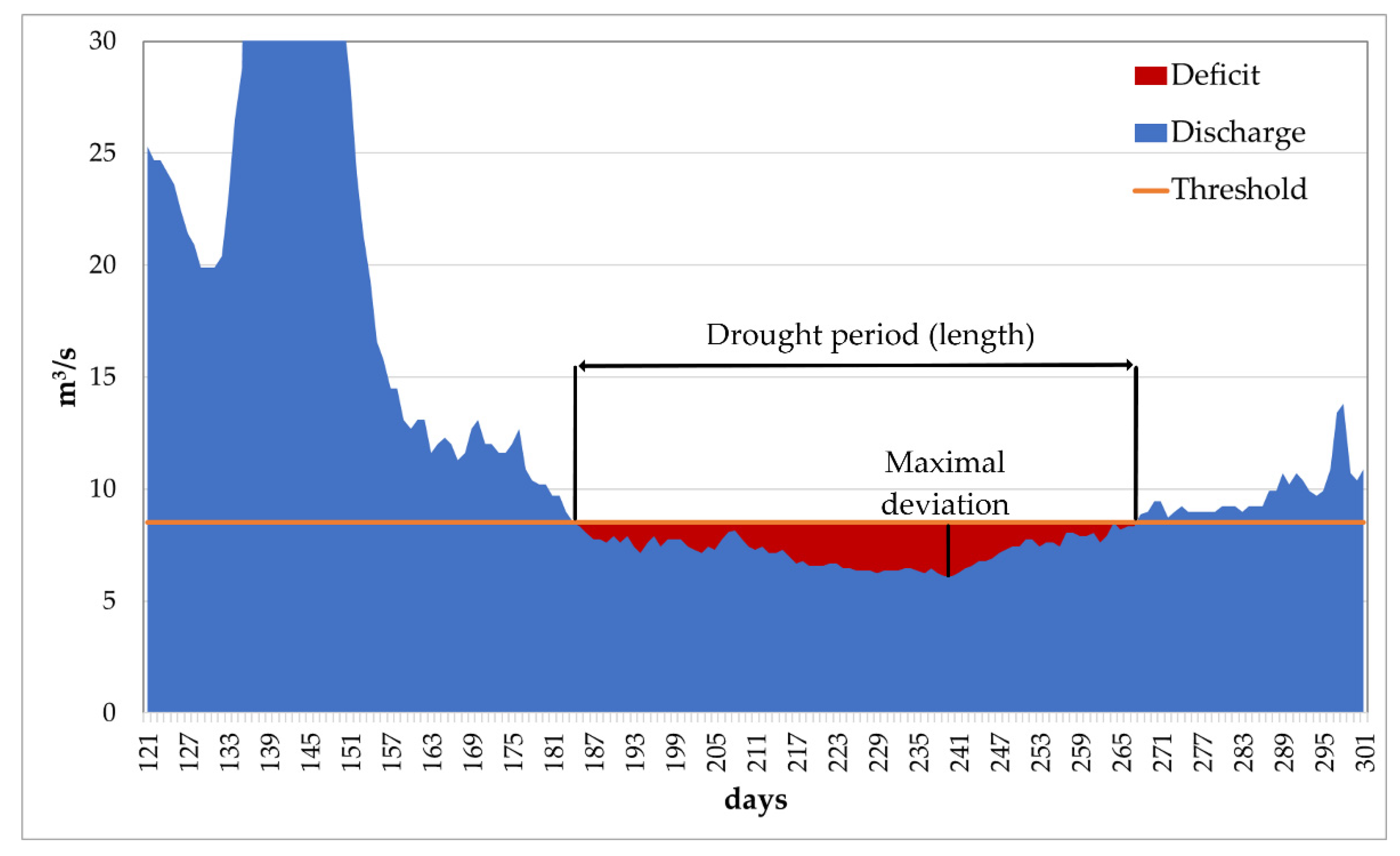
To quantify the information incorporated in hydrographs, the HydroOffice software package [30] was applied. The HydroOffice tool FDC (flow duration curves; version 2.1) is often used to assess low flows. It was selected to calculate 30Q95 and 30Q80. FDC can be created from the entire imported time series or defined parts, such as annual or monthly segments. The HydroOffice tool TLM (threshold level or sequence peak algorithm methods; version 2.1) can be used to evaluate extreme flow conditions. Segments with extreme conditions can be statistically processed and visualized. TLM is designed to assess hydrological drought and flood events. Daily discharge and threshold values were used as input data for calculation with TLM, while drought period (duration), maximum deviation, and deficit volume were obtained as output data (Figure 3).

Maps were created in ArcGIS 10.4 using the Kriging interpolation method (Spatial Analyst toolbox). Kriging assumes that the distance or direction between sample points reflects a spatial correlation that can be used to explain variation in the surface. The Kriging tool fits a mathematical function to a specified number of points, or all within a specified radius, to determine the output value for each location. The general formula for both interpolators is formed as a weighted sum of the data:

$$\widehat{Z}\left(s_0\right)={\displaystyle \sum }_{i=0}^N{\lambda }_{i}Z(s_i)$$

where Z(s_i) is the measured value at the ith location, λ_i—an unknown weight for the measured value at the ith location, s₀—the prediction location, N—the number of measured values. The weight, λ_i, depends solely on the distance to the prediction location. However, with the Kriging method, the weights are based not only on the distance between the measured points and the prediction location, but also on the overall spatial arrangement of the measured points.

The TREND software package (V.1.0.2.) is a standalone product of the CRC for Catchment Hydrology’s (CRCCH) Climate Variability Program designed to facilitate statistical testing of trend, change, and randomness in hydrological time series data [31]. It contains 12 statistical tests based on the WMO/UNESCO Expert Workshop on Trend/Change Detection. This software was used to detect and examine the statistical significance of trends by the Mann–Kendall (MK) and Spearman’s Rho (SR) nonparametric tests. The MK nonparametric test was developed by Mann [32] and Kendall [33] to detect linear or non-linear trends. The SR test is applied to identify the absence of trends [34,35]. The presence and direction of monotonic trends in the data series of 30Q were tested at significance levels α = 0.1 or 0.05 (positive/negative or significant positive/negative, respectively).

3. Results

3.1. Spatial Variability of the Low-Flow Indices

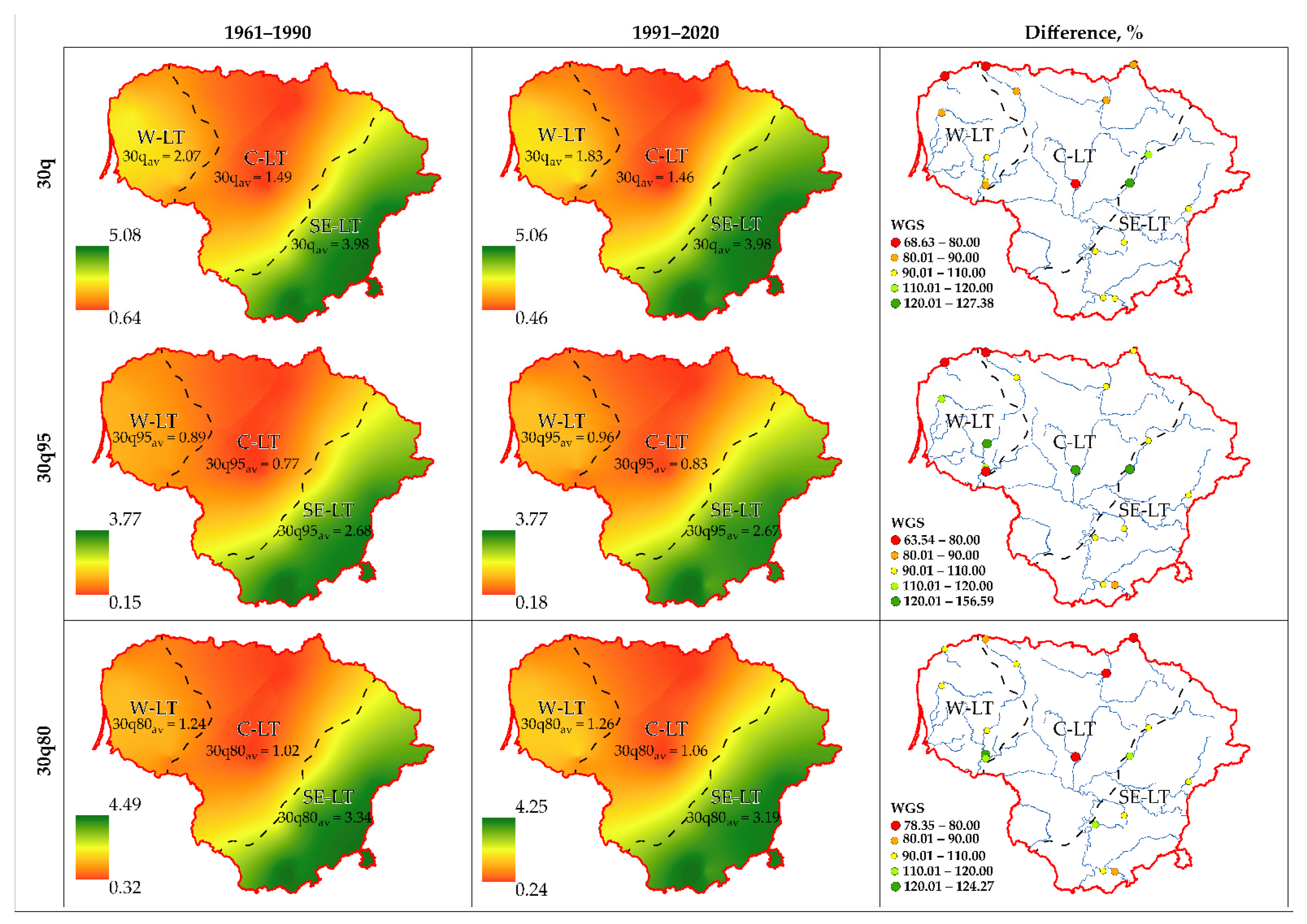
Low flows may occur at any time of the year, depending on the climatic conditions and hydrological processes taking place in the catchment. Regional patterns in low-flow behavior were analyzed using specific low-flow indices (30q, 30q95, and 30q80 (L/s·km²)) for the two selected periods (1961–1990 and 1991–2020) (

Table 2. Low-flow indices by the different regions and periods.

	1961–1990			1991–2020
	30q	30q95	30q80	30q	30q95	30q80
W-LT	1.28–2.63	0.45–1.13	0.75–1.56	1.04–2.32	0.49–1.23	0.74–1.69
C-LT	0.63–3.31	0.15–2.38	0.32–2.71	0.46–3.39	0.18–2.42	0.24–2.91
SE-LT	2.24–5.07	1.20–3.77	1.66–4.84	2.62–5.06	1.51–3.77	1.87–4.25

). In the Southeastern hydrological region (SE-LT), the increase in lower values of all low-flow indices was established by comparing the 1961–1990 and 1991–2020 periods. In the Western hydrological region (W-LT) and the Central hydrological region (C-LT), a different allocation of lower values between selected periods was established, e.g., lower values of 30q decreased, and meanwhile, no clear tendencies in the changes of other indices were identified.

The analysis of the distribution of low-flow indices showed that, in the W-LT region, the 30q average was 2.07 L/s·km² in 1961–1990 and 1.83 L/s·km² in 1991–2020 (Figure 4). There were no pronounced differences between 30q of the selected periods in the C-LT region (1.49 and 1.46 L/s·km², respectively, in two periods) and the SE-LT region (3.97 L/s·km² in both periods). The biggest 30q average was found in the SE-LT region in both periods. The same tendencies were estimated by the other two indices (30q95 and 30q80). Meanwhile, the lowest average values of all three indices in both periods were detected in the C-LT region.

Further details on the established differences of low-flow indices in 17 WGSs in 3 hydrological regions are provided in Figure 5. The figure shows differences in the indices both over time and across regions. The highest indices were estimated in the SE-LT region, and the lowest were in the C-LT region.

In Figure 4, the differences of the low-flow indices between the two periods (1961–1990 and 1991–2020) and three hydrological regions are given as percentages. Only differences greater than 20% were taken into account in the analysis.

In the W-LT region, a significant decrease in 30q (by 27%) over the last thirty years was estimated for BAR. In the C-LT region, for SUS and VEN2, a considerable difference in the decrease in 30q (32% and 29%, respectively) was found. Meanwhile, in the SE-LT region, the most pronounced increase in 30q was detected for SVE2 (27%).

The changes in 30q95 values over time and across different hydrological regions revealed substantial differences between the two periods. In the W-LT region, in AKM, 30q95 increased by 28%; meanwhile, in BAR, it decreased by 37%. In the C-LT region, three WGSs showed significant differences, i.e., in SUS, 30q95 increased by 56%, and in two other WGSs, it decreased (SES (27%) and VEN2 (21%)). In the SE-LT region, 30q95 significantly increased at one WGS (SVE2 by 38%).

Differences in the 30q80 values were also significant. The C-LT region should be singled out as the one where, in almost all WGSs, the 30q80 values decreased (in three of them significantly, i.e., by more than 20%).

In summary, it should be highlighted that the low-flow indices changed the most significantly in the rivers of the C-LT region. For example, in SUS, 30q decreased by 32% and 30q80 decreased by 22%, whereas 30q95 increased by 56%.

To compare the low flows of different rivers, a modular coefficient K of 30Q was calculated for three hydrological regions in different decades (

Table 3. Distribution of K by decades for hydrological regions.

	1961–1970	1971–1980	1981–1990	1991–2000	2001–2010	2011–2020
W-LT	0.80	1.14	1.42	1.04	0.91	0.89
C-LT	0.87	1.08	1.37	0.91	0.93	0.83
SE-LT	0.97	0.92	1.05	0.97	1.07	1.02

). This analysis showed that the modular coefficient varied differently: in the W-LT region, its values were 0.80–1.42; in the C-LT region, they were 0.83–1.37; and in the SE-LT region they were 0.97–1.05. The smallest deviation was detected in the SE-LT region. In all hydrological regions, the highest K was determined in 1981–1990, whereas the lowest values were established in the W-LT region in 1961–1970, in the C-LT region in 2011–2020, and in the SE-LT region in 1971–1980.

3.2. Temporal Analysis of Low Flow Indices

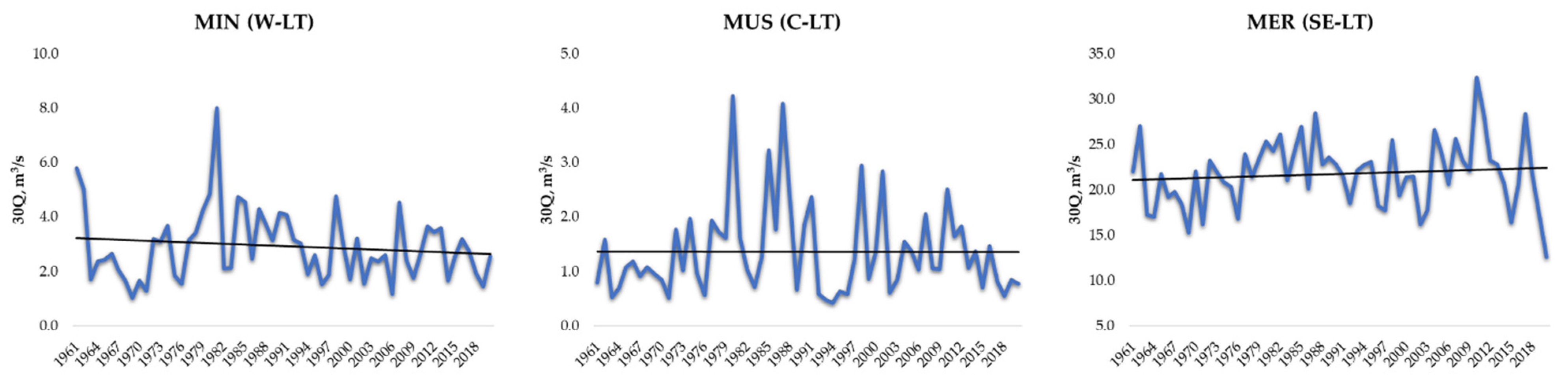
The analysis of 30Q changes in the individual rivers from different hydrological regions (MIN from the W-LT region, MUS from the C-LT region, and MER from the SE-LT region) confirmed the presence of different low-flow patterns in the period 1961–2020 (Figure 6). In the W-LT region, 30Q tended to decrease; on the contrary, 30Q had tendency to increase in the SE-LT region. There was no trend detected in 30Q of MUS from the C-LT region.

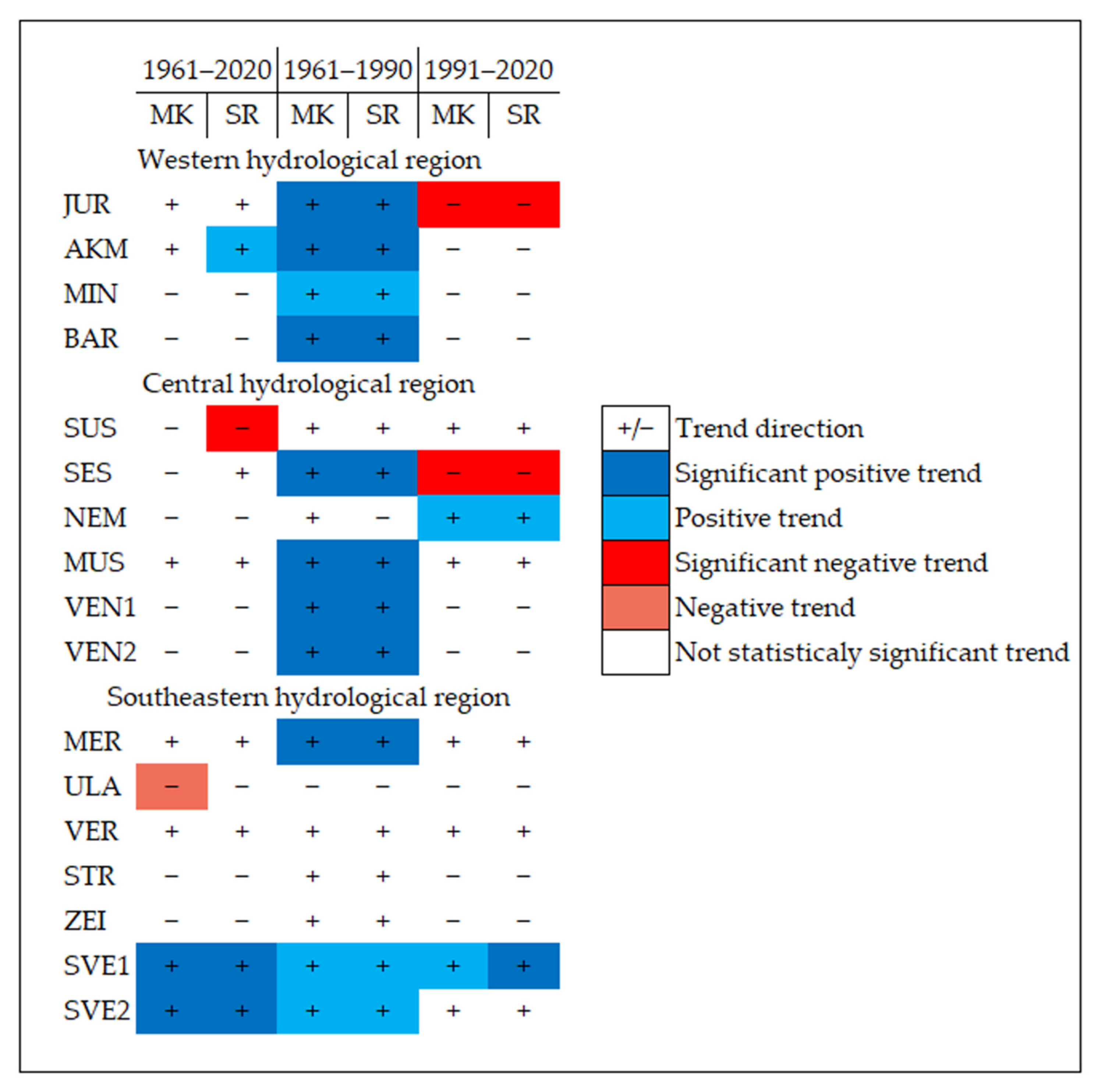
The general behavior of the low-flow (30Q) trend characteristics was assessed for all 17 WGSs using the Mann–Kendall (MK) and Spearman’s Rho (SR) tests over 3 periods (1961–2020, 1961–1990, and 1991–2020). Both tests revealed very similar results (Figure 7). This analysis indicated different trends in different WGSs during the same observation period and in the same hydrological region. It is important to note that no zero-flow values in any low-flow sequence of 30Q were found.

Different tendencies in data of 30Q were detected during the entire observation period and two thirty-year periods. The 30Q values of the longest period (1961–2020) had no trends in the W-LT and C-LT regions (Figure 7). Only in the SE-LT region, significant positive trends of 30Q were identified in two WGSs located on the same river (SVE1 and SVE2). On the opposite, in 1961–1990, trends in 30Q data were significantly positive, and were positive in most rivers, except for a few WGSs, which had no trend (mainly from the SE-LT region). Both tests showed, mostly, no significant trends for the period of 1991–2020, except for one WGS with a significant negative trend in the W-LT region, two WGSs with trends of different significance in the C- LT region, and one WGS in the SE-LT region with a significant negative trend.

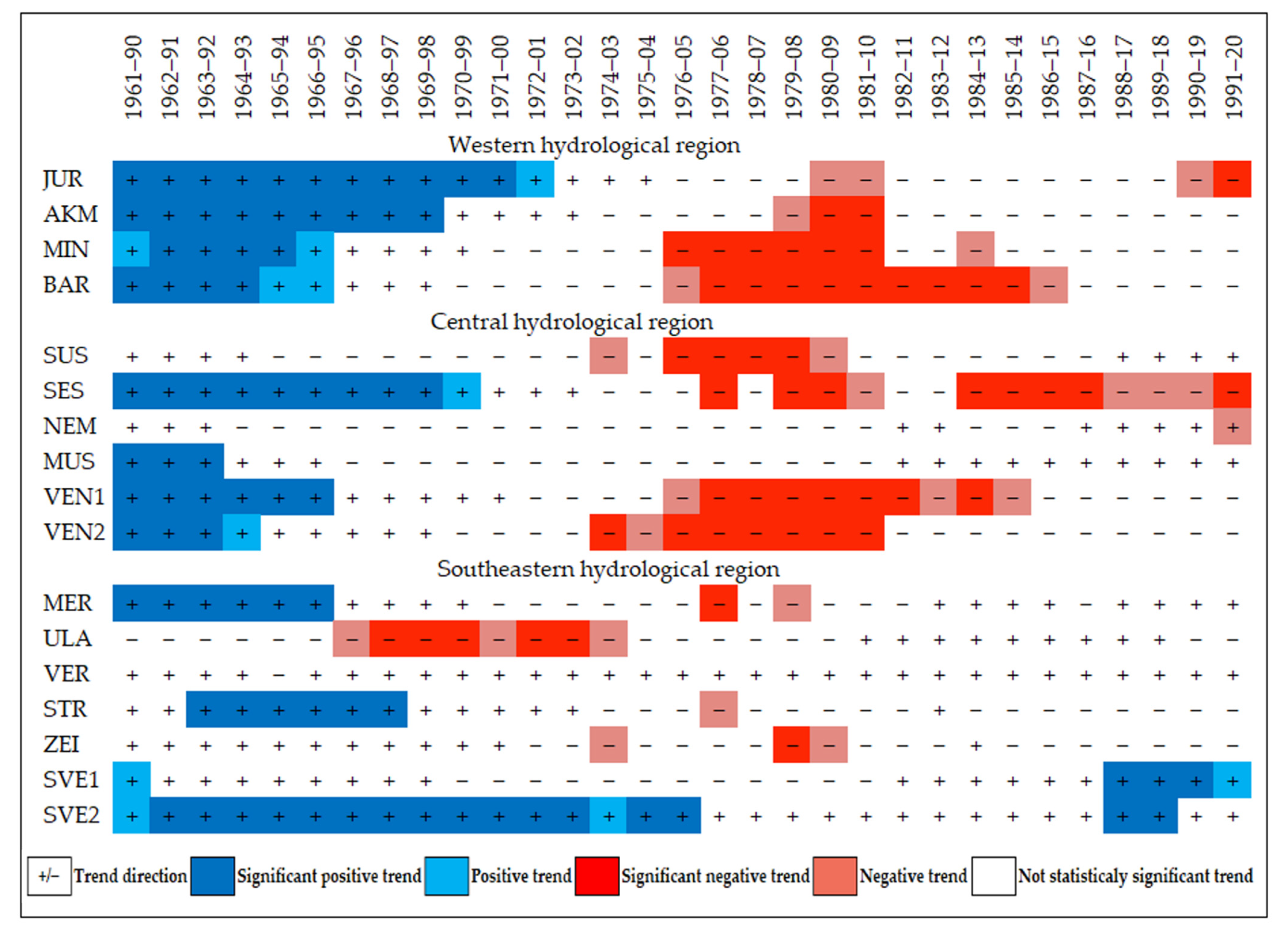
Thirty-year moving averages of 30Q data sets of 17 WGSs were estimated for the period 1961–2020 using the Mann–Kendal test (Figure 8). This approach allows for examining the evolution and dynamics of low flows in a more detailed resolution. In all WGSs, positive or significant positive trends were estimated until 1973, except for one WGS in the SE-LT region with an opposite direction. After 1973, all WGSs in two hydrological regions (W-LT and C-LT) showed negative or significant negative trends. WGSs in the SE-LT region usually did not have significant trends. Moreover, one river with two WGSs had positive or significant positive trends in this region. In contrast, the values of 30Q were significantly increasing in SVE2 (the SE-LT region) until 1976, making it the only WGS with significant increases throughout the whole observation period.

In general, statistically significant positive trends prevailed during the first half of the observation period in the W-LT and C-LT regions, while the negative trends were more concentrated in the middle and at the end of the 1973–2020 period. Meanwhile, WGSs showed different trend directions in the SE-LT region, mainly for the entire observation period.

3.3. Alternations of Duration and Volume of Low Flow

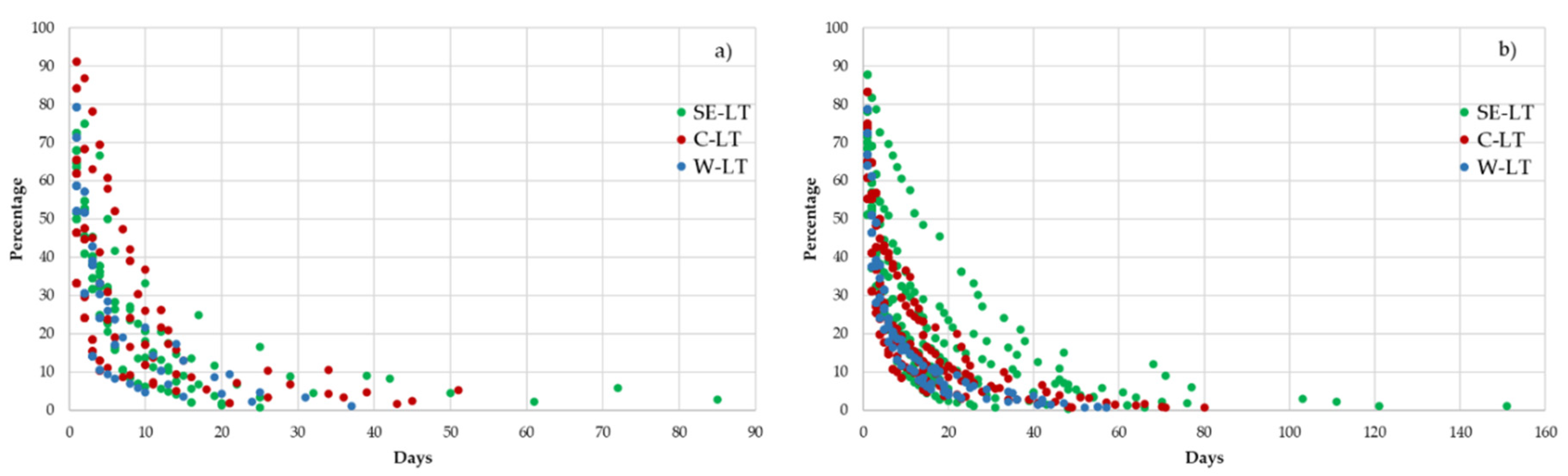
During the analysis of low flow, attention was paid to hydrological droughts, which were determined by two threshold values, namely the indices 30Q95 and 30Q80. For a more detailed analysis of the extreme conditions, drought probability curves were constructed depending on each threshold value for each river (Figure 9a,b). From the obtained graphs, it can be concluded that the duration of droughts increased from the W-LT region to the SE-LT region. This trend can be explained by the impact of different feeding sources in each hydrological region. The rivers of the W-LT region with primary rain feeding were more resistant to prolonged droughts. In the calculations with the threshold value of 30Q95, the highest probability of short droughts (1–2 days) was established in the C-LT region. The longest droughts at the 30Q80 threshold were observed in these rivers: SVE1 was 151 days, SVE2 was 111 and 121 days, ULA was 103 days. With a threshold value of 30Q95, the longest-lasting droughts were observed in these rivers: SVE2 was 72 and 85 days, MER was 61 days.

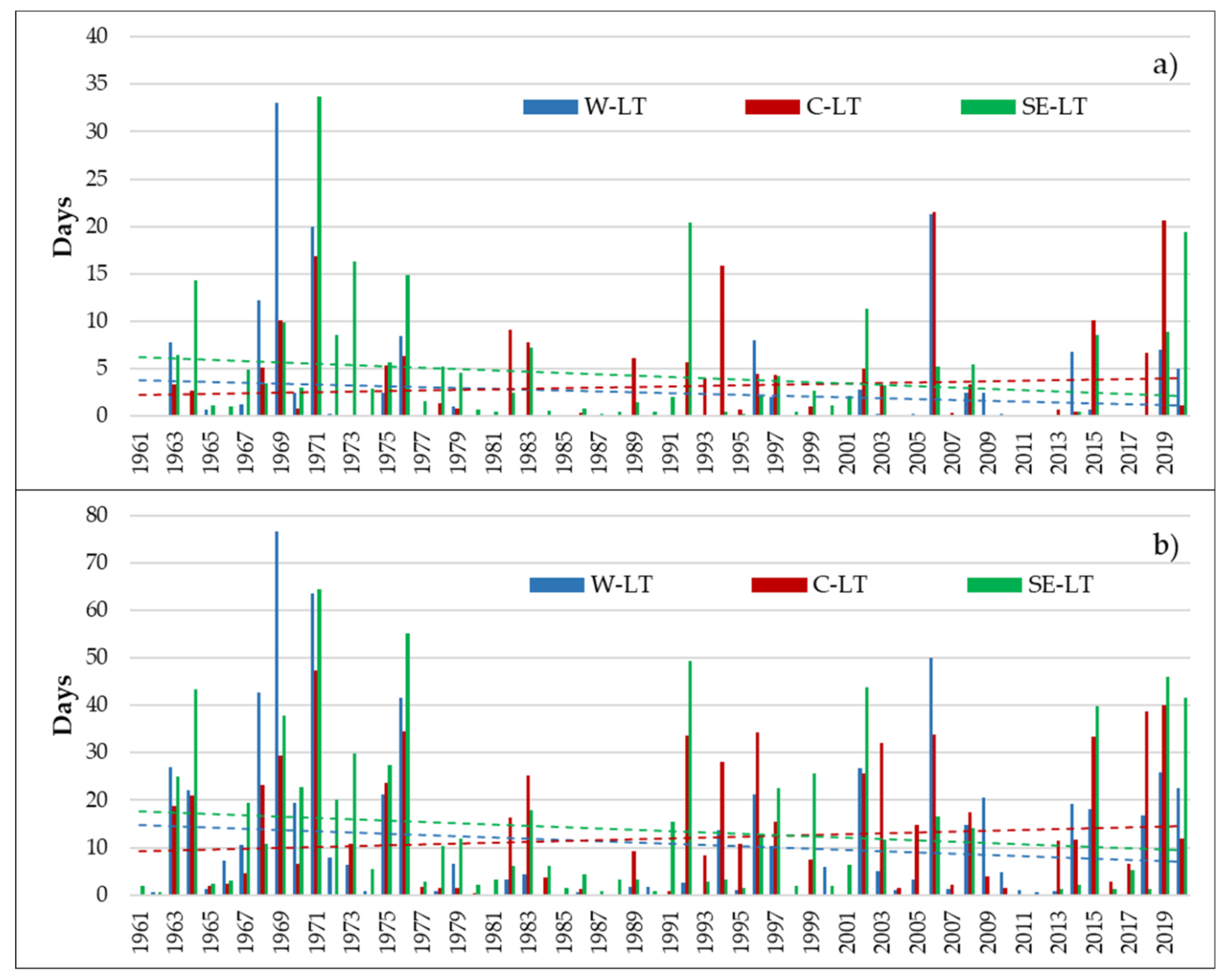
The distribution of dry days over time (Figure 10) showed that, at both thresholds, the average number of dry days per year per river tended to decrease in the W-LT and SE-LT regions, and to increase in the C-LT region. The driest years in Lithuania were 1969 and 1971 (for both thresholds), 1976 (for the 30Q80 threshold), and 2006 (for the 30Q95 threshold). In general, the highest concentration of dry days was observed in the periods 1963–1976, 1992–2006, and 2015–2020. The driest years in the W-LT region were 1969 (33 days for 30Q95, 76.5 days for 30Q80); in the C-LT region, 1971 (47.3 days for 30Q80) and 2006 (21.5 days for 30Q95); in the SE-LT region, 1971 (33.7 days for 30Q95, 64.4 days for 30Q80).

Analysis of annual trends of the deficit of discharge and the number of dry days in each river showed no clear patterns (Figure 11 and Figure 12). In some cases, there was a positive trend towards increasing droughts and a negative trend towards decreasing discharge deficit. For example, in the case of JUR for a threshold value of 30Q95, the mentioned tendencies can indicate a decrease in the deficit of discharge and an increase in dry days. The trends obtained using the two thresholds generally coincided. An exception was ZEI, in which, at the 30Q95 threshold, the duration of droughts and discharge deficits tended to decline, while, at the 30Q80 threshold, the opposite trend was observed.

More detailed information on each river is provided in

Table 4. Changes for 30Q95.

River	Average Deficit during 1961–1990 (103·m3/day)	Average Deficit during 1991–2020 (103·m3/day)	Days with Drought (1961–1990)	Days with Drought (1991–2020)	Flow Deficit during 1961–1990 (103·m3)	Flow Deficit during 1991–2020 (103·m3)	The Lowest Deviation in 1961–1990	The Lowest Deviation in 1991–2020
Western hydrological region
JUR	29.6	15.5	62	49	1834.3	760.3	−1.18	−0.44
AKM	3.9	5.6	117	13	457.9	72.6	−0.14	−0.30
MIN	17.7	14.1	155	96	2751.0	1351.3	−0.74	−0.37
BAR	3.5	5.4	25	79	87.3	426.8	−0.10	−0.28
Central hydrological region
SUS	6.0	5.3	120	59	718.9	312.8	−0.23	−0.12
SES	17.9	17.8	47	138	838.9	2450.3	−0.61	−0.41
NEM	19.2	17.8	99	132	1899.9	2343.2	−0.52	−0.56
MUS	6.9	5.6	69	113	477.8	630.7	−0.29	−0.14
VEN1	11.5	8.5	70	84	805.3	710.2	−0.33	−0.30
VEN2	30.8	45.6	54	131	1660.6	5975.4	−1.05	−1.96
Southeastern hydrological region
MER	53.7	122.6	82	140	4399.5	17,159.0	−2.11	−4.41
ULA	3.0	5.2	4	116	12.1	597.0	−0.05	−0.15
VER	13.0	7.4	191	77	2479.7	570.2	−0.76	−0.24
SRE	12.2	7.3	362	196	4430.6	1435.1	−0.42	−0.41
ZEI	40.0	38.6	46	78	1840.3	3012.8	−1.33	−1.24
SVE1	90.3	48.8	103	58	9295.8	2830.5	−2.34	−1.56
SVE2	79.3	22.3	281	27	22,284.3	603.1	−2.40	−0.64

and

Table 5. Changes for 30Q80.

River	Average Deficit during 1961–1990 (103·m3/day)	Average Deficit during 1991–2020 (103·m3/day)	Days with Drought (1961–1990)	Days with Drought (1991–2020)	Flow Deficit during 1961–1990 (103·m3)	Flow Deficit during 1991–2020 (103·m3)	The Lowest Deviation in 1961–1990	The Lowest Deviation in 1991–2020
Western hydrological region
JUR	16.7	68.2	415	198	6946.6	13,515.6	−1.82	−1.08
AKM	8.7	5.7	491	249	4243.1	1423.9	−0.29	−0.45
MIN	26.8	23.5	358	252	9594.7	5932.2	−1.05	−0.68
BAR	6.9	9.9	207	447	1436.0	4436.6	−0.30	−0.48
Central hydrological region
SUS	10.9	4.9	199	449	2172.1	2202.4	−0.33	−0.22
SES	22.5	31.8	418	471	9409.0	14,982.6	−1.13	−0.93
NEM	33.6	34.9	375	502	12,585.0	17,511.6	−1.10	−1.14
MUS	11.3	11.9	239	381	2702.6	4549.0	−0.46	−0.31
VEN1	18.6	18.7	286	396	5322.2	7420.0	−0.65	−0.62
VEN2	41.0	50.3	192	369	7869.3	18,552.7	−1.67	−2.58
Southeastern hydrological region
MER	126.4	164.0	359	378	45,374.7	61,986.8	−4.33	−6.63
ULA	12.6	21.7	154	586	1941.4	12,694.8	−0.49	−0.59
VER	23.8	17.0	463	291	11,013.4	4952.5	−1.05	−0.53
SRE	15.5	10.4	627	479	9684.6	4996.5	−0.54	−0.53
ZEI	87.3	96.2	319	483	27,841.5	46,453.8	-3.22	−3.13
SVE1	93.2	83.1	448	217	41,760.6	18,030.8	−3.78	−3.00
SVE2	114.1	81.5	733	132	83,650.8	10,752.5	−3.93	−2.17

(for thresholds 30Q95 and 30Q80, respectively). These results confirmed previous findings in the C-LT region—the number of dry days and discharge deficit is higher in the second period—but it should be noted that the depth of droughts (maximum deviation) for some rivers decreased compared to the first period. In the W-LT region, only general trends in the decline of dry days were detected in the second period; all other data were heterogeneous. Only in the case of MIN, the consistency in all drought indices and downward trends in the deficit of discharge and the duration of the drought in the second period at both thresholds were identified. In the rivers of the SE-LT region, no tendencies of decline in the duration or depth of droughts were found.

4. Discussion

The abundant and indisputable scientific evidence that significant climate change is taking place leaves no doubt that low flow is undergoing substantial changes. Therefore, this study intended to provide fresh insight into this phenomenon in Lithuanian rivers, using a long series of available data and more sophisticated methods than previously used.

Two features determine the hydrological regime of Lithuanian rivers. They are all lowland rivers. It is well-known that low-flow formation processes differ in the highlands and lowlands [13,36,37]. Therefore, the Lithuanian river network is expected to have a homogeneous flow behavior. Besides that, catchments in this relatively small country exhibit different hydrological characteristics depending on physico-geographical and climatic (mainly on the distance from the Baltic Sea) conditions. This is the second important feature of Lithuanian river catchments: based on the listed conditions, they are classified into three distinct hydrological regions: Western (W-LT), Central (C-LT), and Southeastern (SE-LT). It is important to mention that since the 1970s, when the first attempt to classify Lithuanian river catchments into regions was made [38], the regional boundaries shifted only slightly [39], and this shift occurred due to climate changes.

For the above reasons, in this study, the regularities of low flow using specific low-flow indices, 30q, 30q95, and 30q80 in rivers in different hydrological regions and over two subperiods (1961–1990 and 1991–2020), were compared and analyzed. The highest indices were estimated throughout the entire observations period in the SE-LT region (30q = 3.97 L/s·km²), and the lowest in the C-LT region (1.47 L/s·km²). In the SE-LT region, the lowest values of indices became less extreme compared to the first subperiod. There were no clearly expressed changes in the river indices of the W-LT and C-LT regions over time.

The trend analysis of 30Q data in rivers from different hydrological regions confirmed the presence of different low-flow patterns in the selected periods, as well. In general, the 30Q values over the entire period (1961–2020) had no trends in all hydrological regions. An exception was one river (from the SE-LT region) having two WGSs (SVE1 and SVE2), where both tests estimated significant positive trends in 1961–2020. In the subperiods, values of the low-flow indices in SVE1 and SVE2 also demonstrated a more or less significant increase. On the opposite, in the first subperiod (1961–1990), trends in 30Q data were significantly positive and positive in most rivers of the W-LT and C-LT regions. Whereas, in the SE-LT region, only a few significant trends were found. The most recent subperiod (1991–2020) can be characterized as having the least pronounced tendencies in the low-flow changes. With some exceptions of more or less significant trends of mixed direction, in the bigger part of WGSs, only a downward direction was identified.

Contrary to expectations, this analysis did not find a significant difference in low-flow characteristics between the regions. Explaining the estimated regularities is a rather complicated task. The fact that no significant changes were observed in the SE-LT region may be related to the runoff fed specifics of the rivers there. Since these rivers are mainly groundwater-fed, it can be argued that despite the ongoing climate change, the low-flow regime of the rivers remains the least affected. The significant positive trends in the first subperiod and slight tendencies of decrease in the second thirty-year period in rivers from other regions might be attributed to climate change, as the river runoff in the W-LT and C-LT regions is more dependent on rain variability [39]. In these regions, estimated thirty-year moving averages in 30Q data in 1961–2020 also showed a decrease in low-flow discharge.

No trends in the annual variation of 30Q over the more extended periods of 1922–2003 and 1941–2003 were detected in the earlier study by Kriaučiūnienė et al. [24]. The identified positive trends in rivers in the W-LT region in 1961–2003 were explained by a very wet period of 1977–1991 in this territory. A similar study of Latvian rivers revealed no statistically significant long-term trends in 30Q of the warm period [23]. The findings of trend analysis of flow indices in Polish rivers [17] demonstrated the existence of some complex spatial gradient. The distance of the catchment centroid from the coast was found to be a very good predictor of trend slopes for most studied indices. In the pan-European study, Stahl et al. [10] found dominant positive trends of low-flow indices around the Baltic Sea.

Over time, the average number of dry days (at both thresholds: 30Q95 and 30Q80) decreased in the W-LT and SE-LT regions and increased in the C-LT region. The identified changes (and the already mentioned lowest specific low-flow indices) in the C-LT region may explain the presence of intermittent rivers. However, the trends in the number of dry days and flow deficit of individual Lithuanian rivers did not help distinguish clear tendencies (e.g., in the study of Bormann and Pinter [16]). In most cases, changes in these two indices went in the same direction; however, the trend of low-flow indices in some rivers was the opposite. The absence of a direct relationship between the two indices shows that low-flow behavior is complex and often catchment-specific.

The most obvious finding to emerge from this study is that the low-flow regime in Lithuanian rivers has changed over time. Similar changes in 30Q in the W-LT and C-LT regions may be related to the predominant surface feeding type of river runoff. In recent decades, the observed decreasing precipitation amount [40] could cause a decrease in low-flow discharges. The estimated increase in the number of dry days in the rivers of the C-LT region may be explained by the decrease in humidity (as the climate becomes less humid moving away from the sea). It has been found that weak infiltration characteristics and high dependence on surface feeding sources (mainly rain and snow) are related to zero-flow phenomena in this region [29]. The differences of low-flow characteristics among the rivers inside the hydrological regions may point to various complex local catchment-specific features that are difficult to include in the investigation. Meanwhile, the absence of a direct link between climatic variables and low-flow events does not indicate that the impact of climate change can be dismissed [36]. Therefore, the present findings showed that it is difficult to establish clear tendencies in the observed low-flow changes over time, and such results are consistent with those obtained in other adjacent and geographically similar catchments. Although in the present study, analyzed river catchments were semi-natural, the potential impact of anthropogenic nature on the identified regularities should not be neglected as well [16,41].

References

- Smakhtin, V.U. Low flow hydrology: A review. J. Hydrol. 2001, 240, 147–186. [Google Scholar] [CrossRef]
- WMO. Manual on Low-Flow Estimation and Prediction; WMO: Geneva, Switzerland, 2008; Available online: https://library.wmo.int/doc_num.php?explnum_id=7699 (accessed on 31 January 2022).
- Poff, N.L.R.; Allan, J.D.; Bain, M.B.; Karr, J.R.; Prestegaard, K.L.; Richter, B.D.; Sparks, R.E.; Stromberg, J.C. The natural flow regime: A paradigm for river conservation and restoration. Bioscience 1997, 47, 769–784. [Google Scholar] [CrossRef]
- Lake, P.S. Ecological effects of perturbation by drought in flowing waters. Freshw. Biol. 2003, 48, 1161–1172. [Google Scholar] [CrossRef]
- Bond, N.R.; Lake, P.S.; Arthington, A.H. The impacts of drought on freshwater ecosystems: An Australian perspective. Hydrobiologia 2008, 600, 3–16. [Google Scholar] [CrossRef] [Green Version]
- Woodward, G.; Perkins, D.M.; Brown, L.E. Climate change and freshwater ecosystems: Impacts across multiple levels of organization. Philos. Trans. R. Soc. B Biol. Sci. 2010, 365, 2093–2106. [Google Scholar] [CrossRef] [Green Version]
- Lennox, R.J.; Crook, D.A.; Moyle, P.B.; Struthers, D.P.; Cooke, S.J. Toward a better understanding of freshwater fish responses to an increasingly drought-stricken world. Rev. Fish Biol. Fish. 2019, 29, 71–92. [Google Scholar] [CrossRef]
- Addressing the Challenge of Water Scarcity and Droughts in the European Union EC Communication from the Commission to the Council and the European Parliament, Addressing the Challenge of Water Scarcity and Droughts in the European Union, Brussels, 18.07.07, COM(2007)414 Final. 2007. Available online: https://eur-lex.europa.eu/LexUriServ/LexUriServ.do?uri=COM:2007:0414:FIN:EN:PDF (accessed on 31 January 2022).
- Intergovernmental Panel on Climate Change (IPCC). Summary for Policymakers. In Climate Change 2021: The Physical Science Basis. Contribution of Working Group I to the Sixth Assessment Report of the Intergovernmental Panel on Climate Change; Masson-Delmotte, V., Zhai, P., Pirani, A., Connors, S.L., Péan, C., Berger, S., Caud, N., Chen, Y., Goldfarb, L.M.I., Huang, M., et al., Eds.; Cambridge University Press: Cambridge, UK, 2021. [Google Scholar]
- Stahl, K.; Hisdal, H.; Hannaford, J.; Tallaksen, L.M.; Van Lanen, H.A.J.; Sauquet, E.; Demuth, S.; Fendekova, M.; Jódar, J. Streamflow trends in Europe: Evidence from a dataset of near-natural catchments. Hydrol. Earth Syst. Sci. 2010, 14, 2367–2382. [Google Scholar] [CrossRef] [Green Version]
- Eisner, S.; Flörke, M.; Chamorro, A.; Daggupati, P.; Donnelly, C.; Huang, J.; Hundecha, Y.; Koch, H.; Kalugin, A.; Krylenko, I.; et al. An ensemble analysis of climate change impacts on streamflow seasonality across 11 large river basins. Clim. Chang. 2017, 141, 401–417. [Google Scholar] [CrossRef]
- Marx, A.; Kumar, R.; Thober, S.; Rakovec, O.; Wanders, N.; Zink, M.; Wood, E.F.; Pan, M.; Sheffield, J.; Samaniego, L. Climate change alters low flows in Europe under global warming of 1.5, 2, and 3 °C. Hydrol. Earth Syst. Sci. 2018, 22, 1017–1032. [Google Scholar] [CrossRef] [Green Version]
- Floriancic, M.G.; Berghuijs, W.R.; Molnar, P.; Kirchner, J.W. Seasonality and Drivers of Low Flows across Europe and the United States. Water Resour. Res. 2021, 57, e2019WR026928. [Google Scholar] [CrossRef]
- Gudmundsson, L.; Boulange, J.; Do, H.X.; Gosling, S.N.; Grillakis, M.G.; Koutroulis, A.G.; Leonard, M.; Liu, J.; Schmied, H.M.; Papadimitriou, L.; et al. Globally observed trends in mean and extreme river flow attributed to climate change. Science 2021, 371, 1159–1162. [Google Scholar] [CrossRef] [PubMed]
- Olden, J.D.; Poff, N.L. Redundancy and the choice of hydrologic indices for characterizing streamflow regimes. River Res. Appl. 2003, 19, 101–121. [Google Scholar] [CrossRef]
- Bormann, H.; Pinter, N. Trends in low flows of German rivers since 1950: Comparability of different low-flow indicators and their spatial patterns. River Res. Appl. 2017, 33, 1191–1204. [Google Scholar] [CrossRef]
- Piniewski, M.; Marcinkowski, P.; Kundzewicz, Z.W. Trend detection in river flow indices in Poland. Acta Geophys. 2018, 66, 347–360. [Google Scholar] [CrossRef] [Green Version]
- Vlach, V.; Ledvinka, O.; Matouskova, M. Changing Low Flow and Streamflow Drought Seasonality in Central European Headwaters. Water 2020, 12, 3575. [Google Scholar] [CrossRef]
- Coch, A.; Mediero, L. Trends in low flows in Spain in the period 1949–2009. Hydrolog. Sci. J. 2016, 61, 568–584. [Google Scholar] [CrossRef]
- Nasr, A.; Bruen, M. Detection of trends in the 7-day sustained low-flow time series of Irish rivers. Hydrolog. Sci. J. 2017, 62, 947–959. [Google Scholar] [CrossRef]
- Hannaford, J.; Marsh, T.J. High and low flow trends in a national network of undisturbed indicator catchments in the UK. In Climate Variability and Change: Hydrological Impacts. Proceedings of the Fifth FRIEND World Conference, Havana, Cuba, 27 November–1 December 2006; International Association of Hydrological Sciences (IAHS) Publ.: Wallingford, UK, 2006. [Google Scholar]
- Kireeva, M.B.; Frolova, N.L.; Winde, F.; Dzhamalov, R.G.; Rets, E.P.; Povalishnikova, E.S.; Pahomova, O.M. Low flow on the rivers of the European part of Russia and its hazards. Geogr. Environ. Sustain. 2016, 9, 33–47. [Google Scholar] [CrossRef] [Green Version]
- Apsite, E.; Rudlapa, I.; Latkovska, I.; Elferts, D. Changes in Latvian river discharge regime at the turn of the century. Hydrol. Res. 2013, 44, 554–569. [Google Scholar] [CrossRef]
- Kriaučiunienė, J.; Kovalenkovienė, M.; Meilutytė-Barauskienė, D. Changes of the low flow in Lithuanian rivers. Environ. Res. Eng. Manag. 2007, 42, 5–12. [Google Scholar]
- Nazarenko, S.; Kriaučiūnienė, J.; Šarauskienė, D.; Jakimavičius, D. Patterns of Past and Future Droughts in Permanent Lowland Rivers. Water 2022, 14, 71. [Google Scholar] [CrossRef]
- Stonevičius, E.; Rimkus, E.; Kažys, J.; Bukantis, A.; Kriaučiūnienė, J.; Akstinas, V.; Jakimavičius, D.; Povilaitis, A.; Ložys, L.; Kesminas, V.; et al. Recent aridity trends and future projections in the Nemunas river basin. Clim. Res. 2018, 75, 143–154. [Google Scholar] [CrossRef]
- Akstinas, V. Low flow projections of the south-eastern Lithuanian rivers in 21st century. In Proceedings of the CYSENI 2016—13th International Conference of Young Scientists on Energy Issues, Kaunas, Lithuania, 26–27 May 2016. [Google Scholar]
- Šarauskienė, D.; Akstinas, V.; Kriaučiūnienė, J.; Jakimavičius, D.; Bukantis, A.; Kažys, J.; Povilaitis, A.; Ložys, L.; Kesminas, V.; Virbickas, T.; et al. Projection of Lithuanian river runoff, temperature and their extremes under climate change. Hydrol. Res. 2018, 49, 344–362. [Google Scholar] [CrossRef]
- Šarauskienė, D.; Akstinas, V.; Nazarenko, S.; Kriaučiūnienė, J.; Jurgelėnaitė, A. Impact of physico-geographical factors and climate variability on flow intermittency in the rivers of water surplus zone. Hydrol. Process 2020, 34, 4727–4739. [Google Scholar] [CrossRef]
- Gregor, M.; Malík, P. RC 4.0 User’s Manual; HydroOffice—Software for Water Science: Bratislava, Slovakia, 2012. [Google Scholar]
- Chlew, F.; Siriwardena, L. TREND—User Guide; CRC for Catchment Hydrology: Canberra, Australia, 2005; Available online: https://toolkit.ewater.org.au/Tools/TREND (accessed on 2 March 2022).
- Mann, H.B. Nonparametric tests against trend. Econometrica 1945, 13, 245–259. [Google Scholar] [CrossRef]
- Kendall, M.G. Rank Correlation Methods; Griffin: London, UK, 1975; ISBN 9780852641996. [Google Scholar]
- Dahmen, E.R.; Hall, M.J.; International Institute for Land Reclamation and Improvement. Screening of Hydrological Data: Tests for Stationarity and Relative Consistency; International Institute for Land Reclamation and Improvement: Wageningen, The Netherlands, 1990; ISBN 9789070754235. [Google Scholar]
- Tonkaz, T.; Çetin, M.; Kâzım, T. The impact of water resources development projects on water vapour pressure trends in a semi-arid region, Turkey. Clim. Chang. 2007, 82, 195–209. [Google Scholar] [CrossRef]
- Raczyński, K.; Dyer, J. Multi-annual and seasonal variability of low-flow river conditions in southeastern Poland. Hydrolog. Sci. J. 2020, 65, 2561–2576. [Google Scholar] [CrossRef]
- Muelchi, R.; Rössler, O.; Schwanbeck, J.; Weingartner, R.; Martius, O. River runoff in Switzerland in a changing climate—changes in moderate extremes and their seasonality. Hydrol. Earth Syst. Sci. 2021, 25, 3577–3594. [Google Scholar] [CrossRef]
- Jablonskis, J.; Janukėnienė, R. Change of Lithuanian River Runoff; Science: Vilnius, Lithuania, 1978. (In Lithuanian) [Google Scholar]
- Akstinas, V.; Šarauskienė, D.; Kriaučiūnienė, J.; Nazarenko, S.; Jakimavičius, D. Spatial and Temporal Changes in Hydrological Regionalization of Lowland Rivers. Int. J. Environ. Res. 2021, 16, 1–14. [Google Scholar] [CrossRef]
- Kriaučiūnienė, J.; Meilutytė-Barauskienė, D.; Reihan, A.; Koltsova, T.; Lizuma, L.; Šarauskienė, D. Variability in temperature, precipitation and river discharge in the Baltic States. Boreal Environ. Res. 2012, 17, 150–162. [Google Scholar]
- Hisdal, H.; Stahl, K.; Tallaksen, L.M.; Demuth, S. Have streamflow droughts in Europe become more severe or frequent? Int. J. Climatol. 2001, 21, 317–333. [Google Scholar] [CrossRef]
Figure 1.
Geographical position (left) and water gauging stations of three hydrological regions of Lithuania (right).
Figure 2.
Low flow indices (example of the Šventoji at Ukmergė WGS in 1973).
Figure 3.
Principal scheme of TLM tool.
Figure 4.
Distribution of low-flow indices (30q, 30q95, 30q80) in the different hydrological regions in 1961–1990 and 1991–2020, and the difference between low-flow indices in the two periods.
Figure 5.
Temporal changes of low-flow indices in three periods: (a) 30q, (b) 30q95, and (c) 30q80.
Figure 6.
30Q variation in different hydrological regions.
Figure 7.
The significance of trends (30Q) by the three periods applying MK and SR tests (red/blue color means that the trend is very significant (α ≤ 0.05), light red/light blue color means that the trend is significant (α ≤ 0.1), no color means that there is no significant trend (α > 0.1)).
Figure 8.
The results of the MK test for 30-year moving averages for 1961–2020 (red/blue color means that the trend is very significant (α ≤ 0.05), light red/ light blue color means that the trend is significant (α ≤ 0.1), no color means that there is no significant trend (α > 0.1)).
Figure 9.
The average number of drought days for the three regions: (a) at threshold 30Q95, (b) at threshold 30Q80.
Figure 10.
The average number of drought days in the three regions: (a) at threshold 30Q95, (b) at threshold 30Q80.
Figure 11.
Examples of drought changes for 30Q95 threshold over time: (a) days with drought in JUR river, (b) deficit volume in JUR river, (c) days with drought in MIN river, (d) deficit volume in MIN river, (e) days with drought in SES river, (f) deficit volume in SES river, (g) days with drought in VEN2 river, (h) deficit volume in VEN2 river, (i) days with drought in VER river, (j) deficit volume in VER river, (k) days with drought in ZEI river, (l) deficit volume in ZEI river.
Figure 12.
Examples of drought changes for 30Q80 threshold over time: (a) days with drought in JUR river, (b) deficit volume in JUR river, (c) days with drought in MIN river, (d) deficit volume in MIN river, (e) days with drought in SES river, (f) deficit volume in SES river, (g) days with drought in VEN2 river, (h) deficit volume in VEN2 river, (i) days with drought in VER river, (j) deficit volume in VER river, (k) days with drought in ZEI river, (l) deficit volume in ZEI river.