
Joint Effects of the DEM Resolution and the Computational Cell Size on the Routing Methods in Hydrological Modelling
by
 , , ,
, , ,
Jingjing Li
1, 
Hua Chen
1,* ,
,
Chong-Yu Xu
2,1,*,
Lu Li
3,
Haoyuan Zhao
1,
Ran Huo
1 and
Jie Chen
1 
1
State Key Laboratory of Water Resources and Hydropower Engineering Science, Wuhan University, Wuhan 430072, China
2
Department of Geosciences, University of Oslo, 0316 Oslo, Norway
3
NORCE Norwegian Research Centre, Bjerknes Centre for Climate Research, Jahnebakken 5, 5007 Bergen, Norway
*
Authors to whom correspondence should be addressed.
Water 2022, 14(5), 797; https://doi.org/10.3390/w14050797
Submission received: 24 January 2022
/
Revised: 20 February 2022
/
Accepted: 28 February 2022
/
Published: 3 March 2022
/
Corrected: 27 May 2022
(This article belongs to the Topic Hydrological Modeling and Engineering: Managing Risk and Uncertainties)
Abstract
:Natural disasters, including droughts and floods, have caused huge losses to mankind. Hydrological modelling is an indispensable tool for obtaining a better understanding of hydrological processes. The DEM-based routing methods, which are widely used in the distributed hydrological models, are sensitive to both the DEM resolution and the computational cell size. Too little work has been devoted to the joint effects of DEM resolution and computational cell size on the routing methods. This study aims to study the joint effects of those two factors on discharge simulation performance with two representative routing methods. The selected methods are the improved aggregated network-response function routing method (I-NRF) and the Liner-reservoir-routing method (LRR). Those two routing methods are combined with two runoff generation models to simulate the discharge. The discharge simulation performance is evaluated under the cross combination of four DEM resolutions (i.e., 90 m, 250 m, 500 m, and 1000 m) and fifty-six computational cell sizes (ranging from 5 arc-min to 60 arc-min). Eleven years of hydroclimatic data from the Jianxi basin (2000–2010) and the Shizhenjie basin (1983–1993) in China are used. The results show that the effects of the DEM resolution and the computational cell size are different on the I-NRF method and the LRR method. The computational cell size has nearly no influence on the performance of the I-NRF methods, while the DEM resolution does. On the contrary, the LRR discharge simulation performance decreases with oscillating values as the computational cell size increases, but is hardly affected by the DEM resolution. Furthermore, the joint effects of the DEM resolution and the computational cell size can be ignored for both routing methods. The results of this study will help to establish the appropriate DEM resolution, computational cell size, and routing method when researchers build hydrological models to predict future disasters.
1. Introduction
Natural disasters bring huge losses to society, ecology, and the economy. Drought and flood events are common natural disasters and have led to significant troubles for humans [1,2,3]. Drought events can cause extreme shortages of domestic water, irrigation water and food, such as the drought that occurred in Southwest China in 2009 [4] and the droughts in eastern Africa in 2011 and 2017 [5], while extreme flood events have also caused casualties and property losses [6,7,8,9].
The development of science and technology [10,11,12,13,14,15] provides the possibility for disaster prevention and control. Studying the natural laws of the basin [16,17] and predicting the hydrometeorological elements of the basin are important measures to prevent natural disasters. Hydrological models play an important role in hydrological simulation and hydrological prediction. The accuracy of the hydrological simulation is affected by many factors, such as the routing methods [18], the accuracy of the input data [19,20], the model parameters [21] and so on [22]. The routing method, which transfers the simulated runoff over the basin into the downstream river discharge in hydrological modelling, plays a vital role in drought and flood prediction. A robust routing method contributes to achieve better discharge simulation results. The fluvial hydraulics model is a satisfactory method to establish the hydraulic hazard maps [23,24]. It simulates detailed flood dynamics at high spatial and temporal resolutions [24]. However, a lot of measured data, including hydrological data and hydraulic data, are needed in hydraulics simulation. Besides, highly sophisticated hydraulic simulations are time consuming [20], especially for large-scale watersheds. In the absence of detailed measured data or for basins of large areas, the DEM-based routing methods, or intelligent algorithms [25], can be alternatives. Conceptual models require less computational effort but they do not take into account the flood inundation and wave diffusion. The growing number of easily accessible gridded meteorological datasets and global Digital Elevation Model (DEM) datasets have facilitated the rapid development and widespread use of DEM-based routing methods. DEM-based routing methods are widely used in flood routing [23,26,27,28]. Samela et al. [23] proposed a DEM-based approach for extracting the flood-prone areas in the ungauged basin. It behaves well in a subcatchment of the Bulbula River in Africa. Li et al. [29] applied two DEM-based routing methods to the distributed Hydrologiska Byråns Vattenbalansavdelning (HBV) model. The discharge simulation performances with the DEM-based routing methods were better than that of the elevation band-based HBV model.
There are two types of DEM-based routing methods: Cell-to-Cell and Source-to-Sink [18,30]. Both are widely used in distributed hydrological models. The Cell-to-Cell method, which is based on both a channel storage equation and a water balance equation, determines the outflow of each cell, using the known inflow and storage at each time step. The outflow of one cell is the inflow of the adjacent downstream cell. These calculations are performed iteratively at each cell until the outflow of the basin is obtained. The main advantage of Cell-to-Cell routing methods is that the discharge is determined at every cell and the runoff is fully distributed over the basin. Cell-to-Cell routing methods are often fairly simple to implement and understand, although the computational demand increases rapidly with the increase in the number of cells [31,32,33,34]. The Source-to-Sink routing method determines how the runoff in each cell independently contributes to the total discharge at the outlet of the basin. Most Source-to-Sink routing methods are more computationally efficient than the Cell-to-Cell methods and are more widely applicable in various disciplines [30,35,36,37].
Generally, runoff is routed through flow nets identified from DEM data, in both the Cell-to-Cell and Source-to-Sink routing methods. Due to computational limitations in large-scale (i.e., large watershed, national or global) hydrological models, routing is often performed with computational cell resolutions that are coarser than those found in the DEMs.
In practice, the computational cell size may vary widely within a given model, depending on the spatial domain of the model works; while relatively coarser computational cell sizes may be used for simulating continental-scale basins, finer computational cell sizes are expected to improve the accuracy of the calibrated parameters and the model results. In regional and global hydrological modelling, the computational cell size usually ranges from 0.1° 0.1° (about 10 km ) to 5 5 (about 500 km 500 km). For example, Harrigan et al. [38] simulated discharge at 1801 discharge stations, using the LISFLOOD routing model [39] and the ERA5 global runoff reanalysis dataset, which has a resolution of 0.1° × 0.1° [40]. Xie et al. [41] conducted a regional parameter estimation in China, using the Variable Infiltration Capacity (VIC) model at a resolution of 50 km 50 km. Niu et al. [42] simulated the discharge based on the flow net at a resolution of 1 1 in 16 catchments in the Pearl River Basin in China. Just as there are various computational cell size options, the typical DEM resolutions in hydrological modelling range from 15 m 15 m to 1 km 1 km. While finer DEM data resolutions are desirable, in practice, the preferred DEM resolution must be balanced against the available computational resources, especially in large-scale hydrological simulation. If the computational costs are too high, or if there is a lack of high-resolution DEM data for a given study area, it may make more sense to use a coarser DEM dataset.
The DEM dataset resolution and the computational cell size affect the routing method performance at the same time, and the user must carefully select the appropriate computational cell size and DEM resolution for their specific situation. While numerous studies have examined how the two conditions affect the modelling results separately [43,44], there is very little information about how they jointly affect the routing method performance. Using two different computational cell sizes of 25 km and 350 km, Arora et al. [45] explored how the computational cell size influenced the routing method results (one is for coupled general circulation models at the global scale and the other is for hydrological applications at basin scale). Overall, coarser computational cells resulted in poorer performances. Furthermore, Gong et al. [18] found that, in a water and snow balance modelling system (WASMOD) model of the Dongjiang Basin, the aggregated network-response function (NRF) performed similarly over a variety of computational cell sizes; conversely, the performance of the linear-reservoir-routing method (LRR) decreased with a zigzag pattern as the computational cell size increased. The DEM resolution influenced numerous hydrological parameters, such as the slope, the routing length, the flow net, and, consequently, the simulated discharge [46]. Using DEM resolutions of 100 m, 200 m, and 300 m, Du et al. [44] investigated the effects of the DEM resolution on the simulated storm runoff in a time variant spatially distributed travel time method, which showed that the performance was poor when the DEM resolution was larger than 200 m. Gong et al. [35] demonstrated that the simulated discharge, using the NRF routing method, was relatively insensitive to the DEM resolution differences between the Hydroshed (about 90 m) and Hydro1k (1000 m) datasets. Jeon et al. [47] studied the discharge results and processing time in the Heukcheon Basin for various DEM resolutions (15 m, 30 m, 70 m, 100 m, 200 m, and 300 m) and found that the largest acceptable DEM resolution was 100 m for a basin with a drainage area of ~300 km2. Chaubey et al. [48] found that to get less than 10% bias in Soil and Water Assessment Tool (SWAT) output for total phosphorus (TP), discharge, and NO3-N simulation, the adequate DEM resolution should be between 100 m and 200 m. While these studies provide valuable information about the effects of the computational cell size and the DEM dataset resolution individually, the joint effect of DEM resolution and computational cell size on modelling performance is yet to be studied.
Finer DEM resolution and finer computational cell size can better capture the basin microtopographic features in hydrological modelling. However, it also means larger computational complexity and longer calculation time for distributed hydrological models. Thus, researchers must find a balance between modelling efficiency/accuracy and the required DEM resolution and the computational cell size. On the premise of ensuring the results of the runoff simulation, the shortest possible runoff simulation time and the smallest workload are pursued. This study, therefore, aims to investigate how DEM resolution and computational cell size jointly affect the performance of routing methods in terms of discharge simulation in distributed hydrological models. Two representative routing methods are selected in this study, including the Liner-reservoir-routing method (LRR), and the improved aggregated network-response function routing method (I-NRF) [49]. LRR is a typical Cell-to-Cell routing method and I-NRF is a typical Source-to-Sink routing method. Two rainy basins with different areas are used in this study. This study can help researchers to choose the most appropriate modelling approach based on the existing data and computation services when predicting drought and flood disasters. In the rest of this paper, Section 2 describes the study area and the data, Section 3 presents a detailed description of the methods and Section 4 presents our results. Then, the conclusions are drawn in Section 5.
2. Study Area and Data
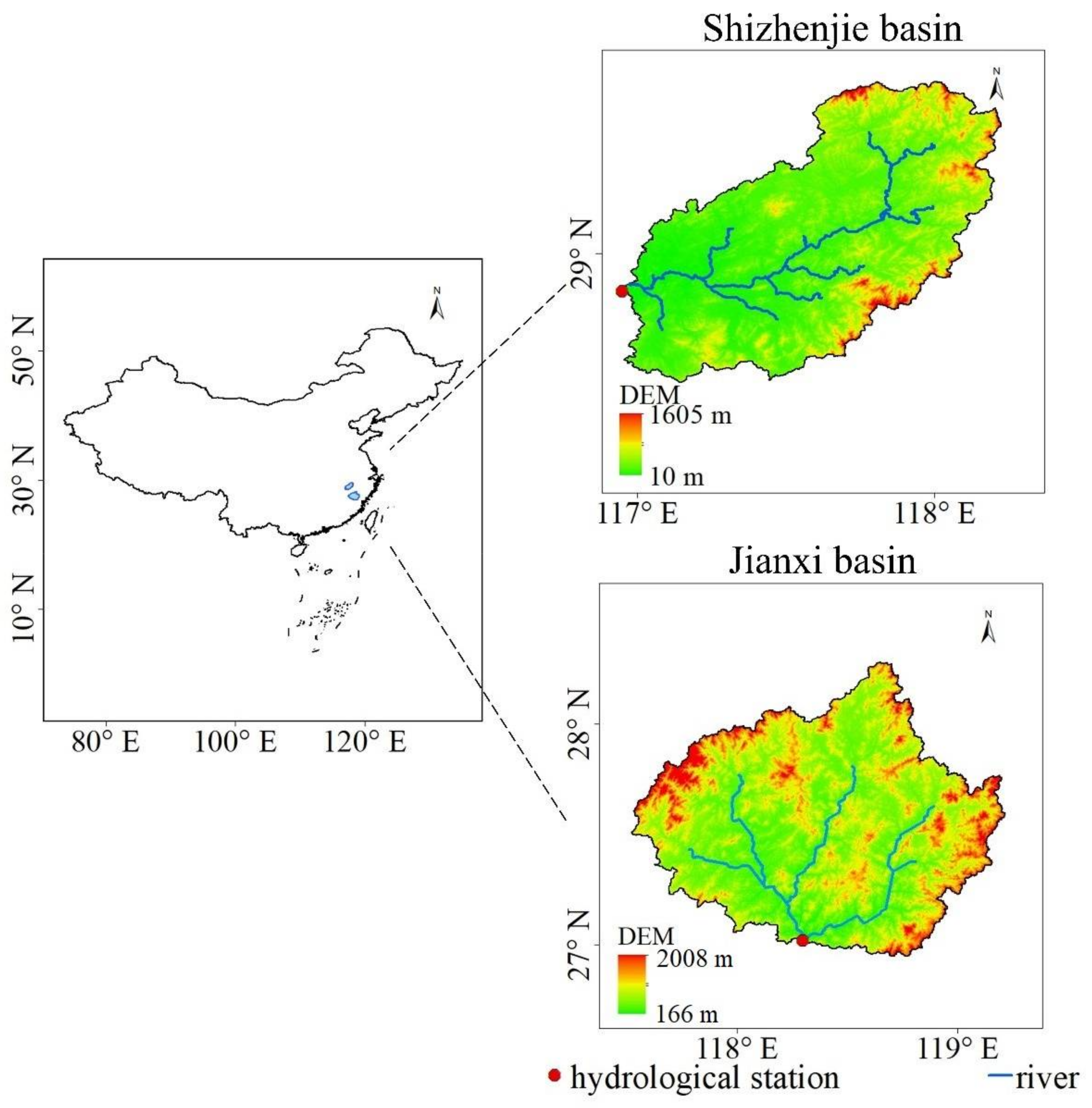
Two basins with different areas are selected to test the generality of the results, namely the Jianxi basin and Shizhenjie basin in southeast China. The Jianxi basin is approximately twice the size of the Shizhenjie basin. The Jianxi River basin (26°31′–28°31′ N, 117°31′–119°00′ W) is the largest tributary in the upper reaches of the Minjiang River, with a drainage area of 14,898 km2 above the Qilijie station. Qilijie station is located at the outlet of Jianxi River. The elevation of the Jianxi basin ranges from 166 m to 2008 m (a.m.s.l.). The Lean River has a drainage area of 8294 km2 above Shizhenjie station. Shizhenjie station is located downstream of Lean River. In the Shizhenjie basin (28°56′–29°58′ N, 116°94′–118°23′ W), the elevation ranges from 10 m to 1605 m (a.m.s.l.). The drainage net and terrain of our two study areas are shown in Figure 1.
DEM datasets with four different resolutions are used: 1000 m [50], 500 m (http://www.resdc.cn/data.aspx?DATAID=123 (accessed on 14 January 2022)), 250 m (http://www.resdc.cn/data.aspx?DATAID=123 (accessed on 14 January 2022)), and 90 m (http://www.resdc.cn/data.aspx?DATAID=123 (accessed on 14 January 2022)). The daily precipitation, air temperature, and relative humidity data are provided by the National Meteorological Information Centre in China. The daily discharge data of the Qilijie hydrological station in the Jianxi basin from 2000 to 2010 was obtained from the Fujian Hydrology Bureau, and the daily discharge data of the Shizhenjie hydrological station from 1983 to 1993 was provided by the Bureau of Hydrology of the Changjiang Water Resources Commission.
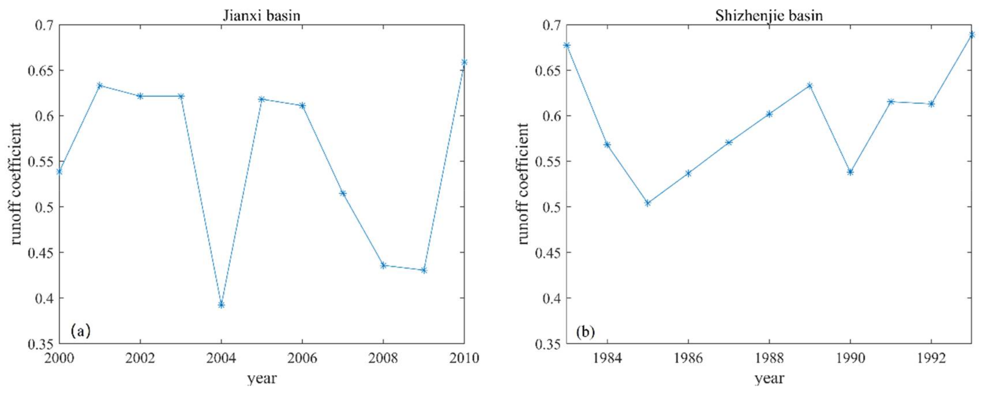
The Long-Range Dependence of the hydroclimatic variables is important in hydrological modelling [51]. Thus, the statistical characteristics of the daily precipitation, air temperature, relative humidity and discharge for the tested period in the study area are calculated and shown in Table 1. Four important statistical moments [51] are used in this study: the mean, standard deviation, skewness coefficient and kurtosis coefficient. Figure 2 shows the change in the runoff coefficient in the tested period.
3. Methods
3.1. Routing Methods
3.1.1. The Improved Aggregated Network-Response Function Routing Method
I-NRF [49], the improved version of NRF, achieves accurate simulation of discharge results in many basins. It is a typical Source-to-Sink routing method. The I-NRF routing method relies on slope and routing length data extracted from the grids of the DEM dataset:
where (minute) is the travel time between each grid and the outlet, k (-) is the total number of grids on the flow path, is the slope, (m) is the routing length between each grid and the downstream grid, and () is the slope threshold that prevents the occurrence of an infinite parameter value. Parameter (m/s) is the wave velocity in the grid with a slope of 45 and b (-) is a parameter that reflects how sensitive the wave velocity is to the slope. These two routing parameters and b both require special calibration.
3.1.2. Linear Reservoir Routing Method
Based on the characteristic river length theory, the linear reservoir routing (LRR) method, which is a Cell-to-Cell routing method, is popular and reliable [18]. The LRR algorithm is defined as:
where I1 (m3/s) and Q1 (m3/s) are the inflow and outflow at the start time, I2 (m3/s) and Q2 (m3/s) are the inflow and outflow at the end time, and (s) is the calculation time. Kl (s) is a constant that represents the time needed to travel through the characteristic river length, l (m) is the length of the river section, and v (m/s) is the wave velocity of the flood. Of these parameters, only v requires calibration.
The key routing parameters for the I-NRF and LRR routing methods are shown in Table 2.
The LRR routing method needs to satisfy the Courant criterion [52]. The Courant number is defined as:
where Courant is Courant number, u is the wave velocity, dt is the time step, dx is the cell size.
To avoid getting wrong discharge simulation performance, the computational Courant number should satisfy the following criteria:
In this study, daily discharge at the hydrological station is used to compare with the simulated e. However, the running time step is set to be 1/20 day when the LRR routing method is used for all computational cell sizes.
The maximum wave velocity and minimum computational cell size that appeared in this article are used to calculate the maximum Courant number in this article.
The Courant number is always less than 1 so that the change in the computational cell size does not cause the model to violate the courter number with the LRR routing method.
3.2. Runoff Generation Models
3.2.1. SIMHYD
In this study, two runoff generation models are selected to test the generality of the result. The conceptual daily rainfall-runoff model SIMHYD [53,54] is employed as one of our runoff generation models. This model has been previously applied in numerous study areas, including China [53,55,56,57]. For more information on the model algorithm, refer to Chiew et al. [53]. The details of the seven model parameters in the SIMHYD model are shown in Table 3.
3.2.2. Water and Snow Balance Modelling System (WASMOD)
The second model used in the study is the water and snow balance modelling system (WASMOD) [58]. WASMOD is a popular model that has been used in many study areas worldwide [59,60,61,62]. The version of WASMOD used in this study is that of Widén Nilsson et al. [62], which consists of only three parameters and no snow module. The parameters for this version of WASMOD are listed in Table 4. Compared to the equations listed in Widén Nilsson et al. [62], two additional parameters are added. Parameter corrects the precipitation bias that arises due to a lack of snow measurements that occur occasionally at higher altitude areas and is described in the potential evaporation calculation equation ( is not needed when data are available):
where (mmday−1) is the potential evaporation, () is the temperature, and (-) is the relative humidity, (mm day−1 −2) is the parameter.
3.3. Different Computational Cell Sizes and Interpolation Method
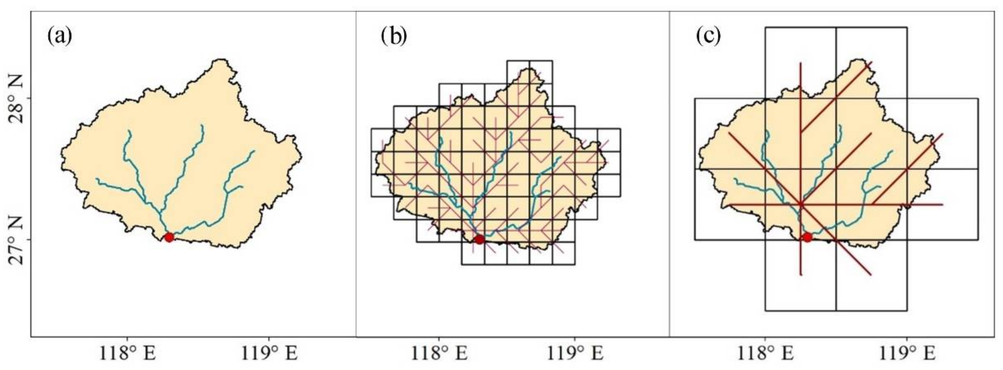
Following the boundary of the study basin, computational cells for routing methods are generated. The computational cell sizes range from 5 arc-min to 60 arc-min with an interval of 1 arc-min, resulting in a total of 56 cell sizes. For illustration purposes, the computational cells of Jianxi basin at the resolution of 10′ and 30′ are shown in Figure 3. The computational cell is constructed according to the following principle: the leftmost longitude of the cells is the same as the integer part of the leftmost latitude of the basin boundary and the bottom latitude of the cell is the same as the integer part of the bottom latitude of the watershed boundary. To maintain the water balance, the area of each cell is the area of the basin belonging to this cell. It can avoid the area errors for the boundary cells [18]. After generating the computational cells, extract the flow net at the same resolution of computational cell size using the network scaling algorithm (NSA) [63] (Figure 3).
In order to match the resolution of the meteorological data recorded at the hydrological station with the various computational cell sizes, the Inverse Distance Weighted (IDW) method [64] is employed to interpolate the data to the grid with a resolution of 1 km. For each grid, the distance from the grid center to all hydroclimatic stations is calculated. The four stations closest to the center of the grid are selected to calculate the hydroclimatic data values for this grid. The equations are as follows:
where i is the corresponding number of the 4 stations which are the closest stations to the grid center, weight is the weight of the station data, data_observation is the measured data of the station, and data_g is the hydroclimatic data of the grid.
Using the linear average method, the interpolated meteorological data are then aggregated into the gridded data with the resolution that matches that of the computational cell size. For each cell, the hydroclimatic data value is calculated based on the grids which are belonging to the cell.
where data_c is hydroclimatic data of the cell, j is the corresponding number of the grids belonging to the cell.
3.4. Calibration Algorithms
Two calibration algorithms are used in this study: the Monte Carlo algorithm [65] and the Covariance Matrix Adaption Evolution Strategy (CMA-ES) [66]. Since the available data are not long enough, the calibration period length is set as 7 years and the validation period is set as 4 years according to Klemeš [67]. Besides, the warming-up period equals 1 year in this study. The detailed information on the runoff generation and routing parameters that require calibration are listed in Table 2, Table 3 and Table 4.
The Nash–Sutcliffe efficiency (NSE) [68] is used for model calibration criterion, percentage bias (PBIAS) [69] is also used for results evaluation and comparison.
where (m3/s) is the observed discharge, (m3/s) is the mean observed discharge, (m3/s) is the simulated discharge, and n (day) is the length of the time step.
3.5. Experimental Design
There are a total of 1792 experiments in this study based on the cross combination of two study basins, two routing methods, two runoff generation models, four DEM resolutions and fifty-six computational cell sizes.
3.5.1. Optimal Routing Parameters
In this study, according to the characteristics of the routing method, the Monte Carlo algorithm is used to calibrate the optimal I-NRF routing parameters, and the CMA-ES algorithm is used to calibrate the optimal LRR routing parameters.
The routing parameters are mostly related to basin physical characteristics such as the topography and the underlying surface. As such, it is assumed that the I-NRF and LRR routing parameters are independent of the parameters from the runoff generation models.
Calibration of I-NRF Routing Parameters
The calibration process for the I-NRF routing parameters consists of four steps:
- Several initial routing parameter sets are drafted. For the I-NRF routing method, there are two parameters to be calibrated. Table 2 defines 49 initial routing parameter set values. The number of the initial values is m (m = 1~49).
- The optimal simulation performance for each initial routing parameter for a given DEM resolution and a given computational cell size is calculated using Monte Carlo calibration algorithm. The optimal model performance for each parameter set is denoted as , where i corresponds to the DEM resolution and j corresponds to the computational cell size. Then 48 values using the four different DEM dataset resolutions (i = 1–4) and the 12 computational cell sizes (5 arc-min to 60 arc-min with an interval of 5 arc-min) (j = 1–12) are obtained. In the calibration process, 300 runoff generation parameter arrays are produced as the model input by Latin-Hypercube sampling [70] according to the initial parameter range (Table 4). The applied marginal distribution is the uniform distribution.
- The comprehensive simulation performance for each initial routing parameter set of each DEM resolution () is calculated, where .
- The optimal routing parameter set is selected from the initial routing parameter sets. For each DEM resolution, the optimal routing parameter set for a given basin is selected using as a criterion and listed in Table 5.
Calibration of LRR Routing Parameters
The CMA-ES algorithm is used to identify the optimal routing parameters for the LRR routing method.
The calculation of the optimal LRR routing parameters happens in four stages:
- Several initial routing parameters are drafted. For the LRR routing method, there is only one parameter to be calibrated. Table 2 defines 6 initial values. The number of the initial values is n (n = 1–6).
- The optimal simulation performance for each routing parameter for a given DEM resolution and a given computational cell size is calculated using CMA-ES algorithm, denoted as . With 4 DEM resolutions (i = 1–4) and 12 computational cell sizes (5 arc-min to 60 arc-min with an interval of 5 arc-min) (j = 1–12), 48 values are obtained. In the calibration process, the initial range of runoff generation parameters is given in Table 4.
- The comprehensive simulation performance () for each parameter of each DEM resolution is calculated. Here, .
- The optimal routing parameter is selected from the initial routing parameters. For each DEM resolution, the optimal routing parameter set for the basin is selected using as a criterion and the results are listed in Table 5.
3.5.2. Optimal Runoff Generation Parameters
As mentioned above, there are a total of 1792 experiments. Once the optimal routing parameters are obtained and fixed, the runoff generation parameters are calibrated in each experiment using the CMA-ES algorithm [66]. Then the corresponding NSE values are ultimately obtained (Figure 4, Figure 5 and Figure 6) for 1792 experimental simulations.
4. Results
4.1. The Effect of Computational Cell Size on the Discharge Simulation Performance
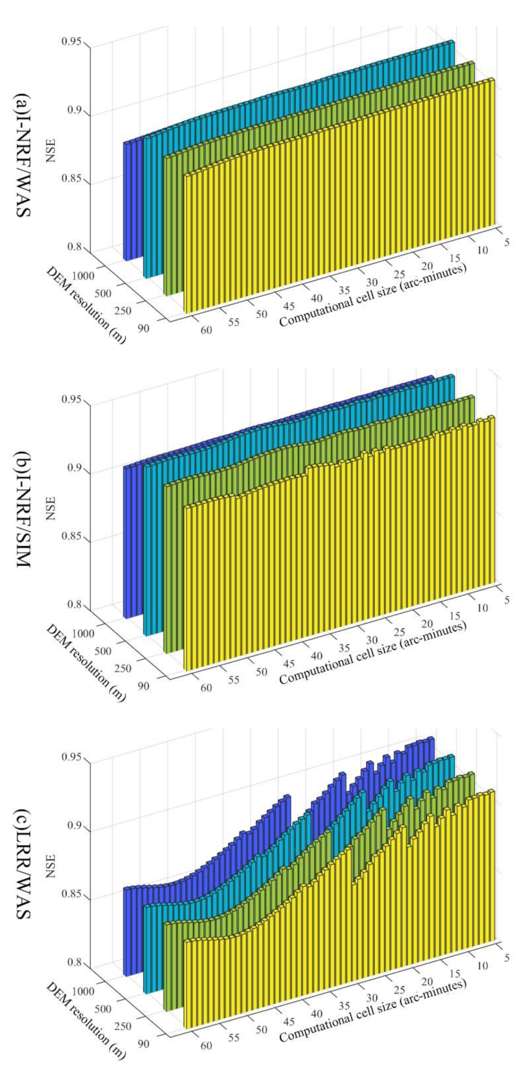
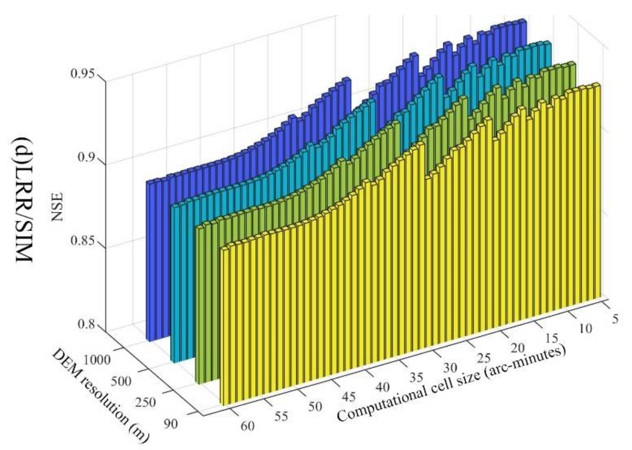
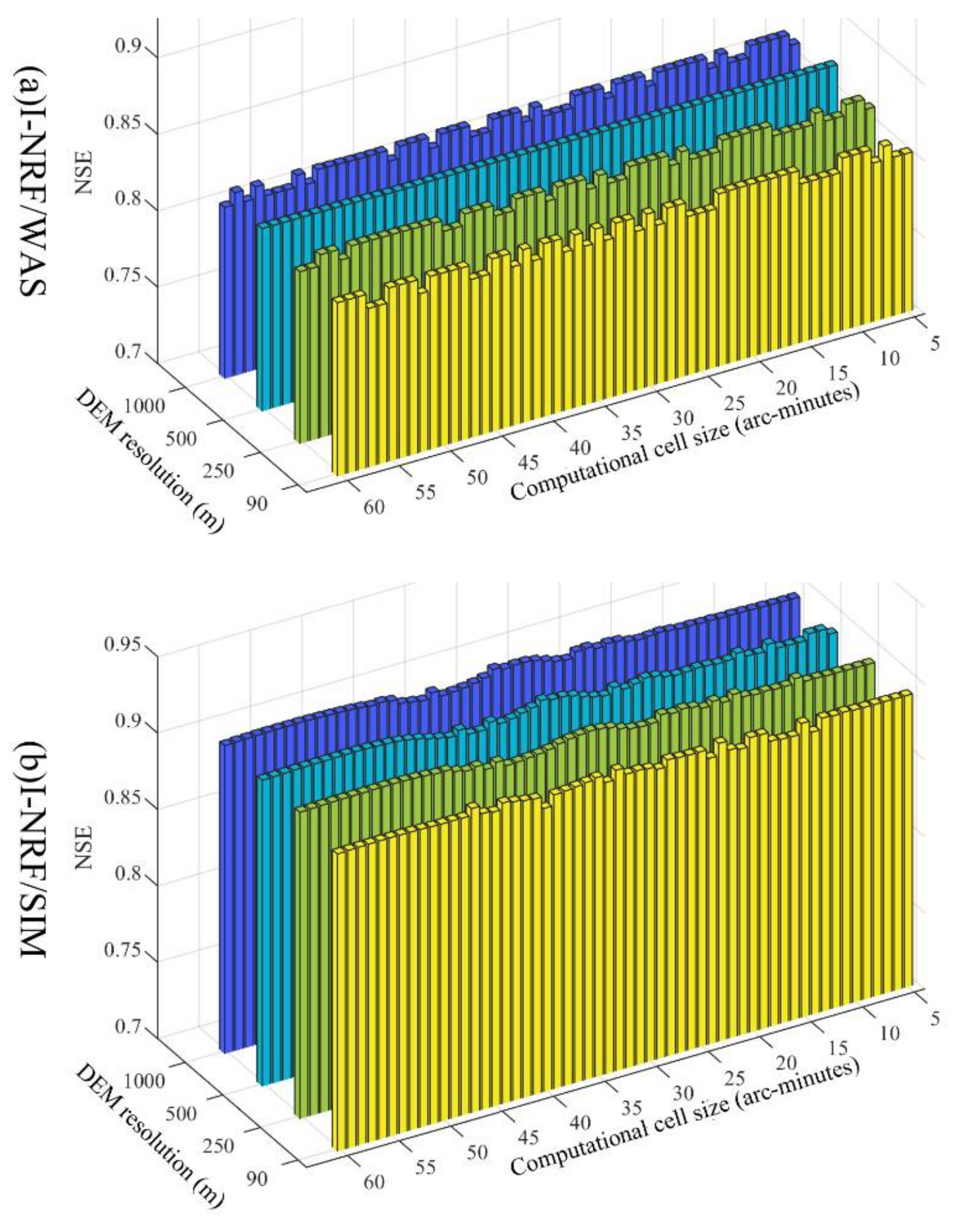
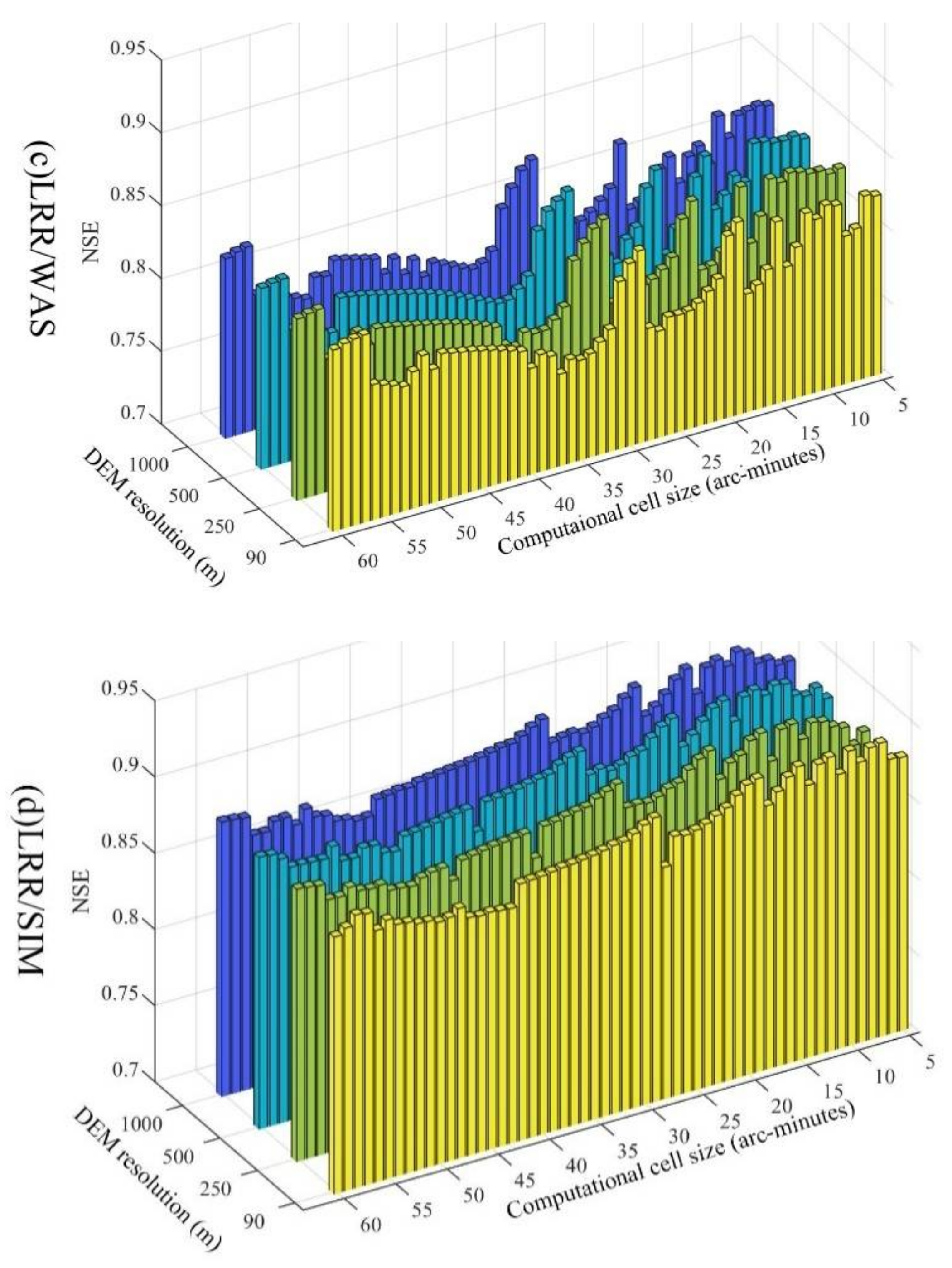
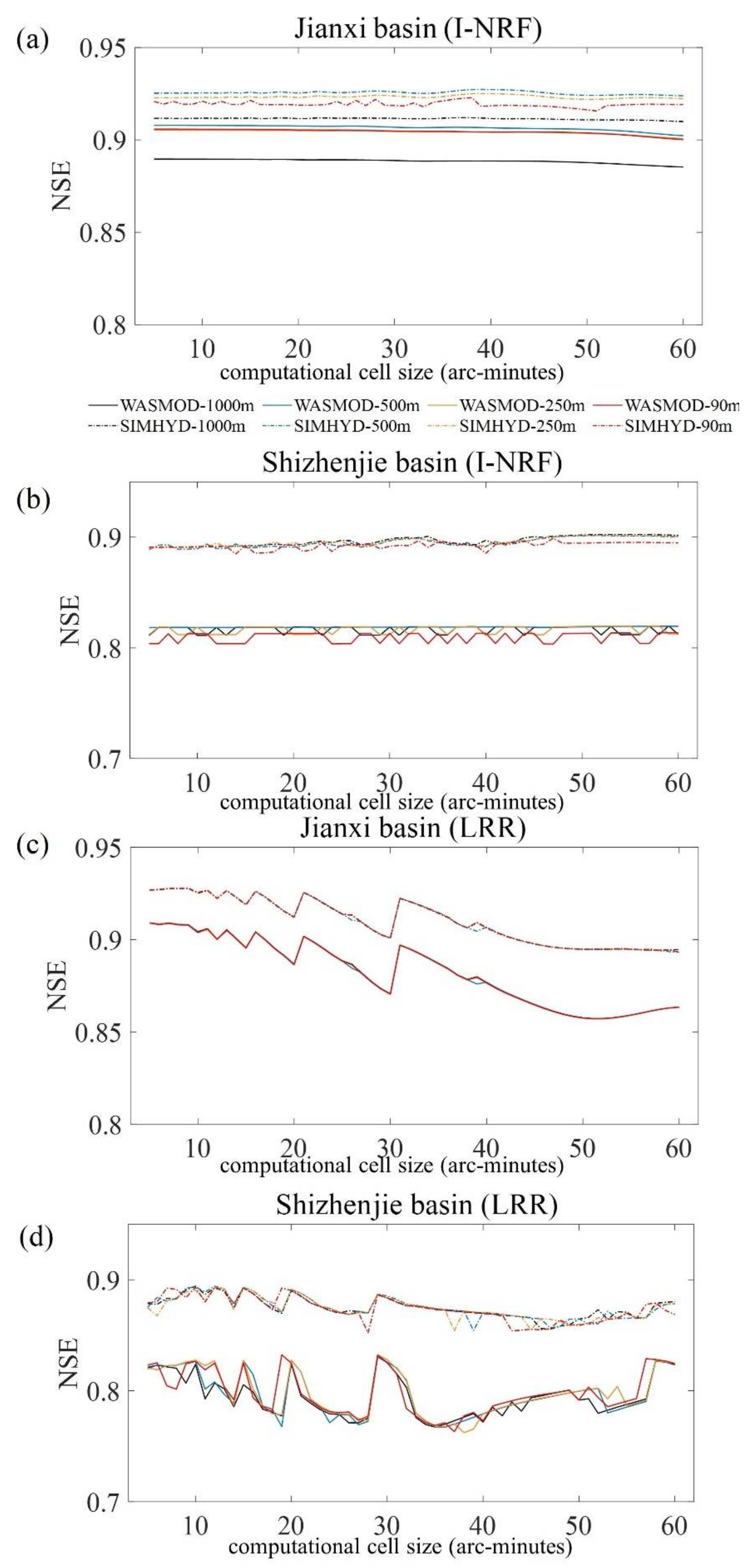
The NSE values for the various DEM resolutions (x-axis) and computational cell sizes (y-axis) for both routing methods in Jianxi basin and Shizhenjie basin are shown in Figure 4 and Figure 5. To improve readability, line charts of NSE are shown in Figure 6.
Figure 4, Figure 5 and Figure 6 show that the discharge simulation performance curve for the Jianxi basin, as computational cell size changes, is mostly a straight line. While the WASMOD model generates some noise in the NSE values of the Shizhenjie basin (Figure 5a,b and Figure 6b), the NSE values are mostly constant, despite the changing computational cell sizes. In general, the discharge simulation performance with the I-NRF routing method stays stable, regardless of the computational cell size. Gong et al. [18] discussed in detail why NRF discharge simulation performance is scale-independent. I-NRF, the improved version of NRF, retains the scale-independency characteristic of NRF. This scale-independency is produced by the algorithm, in which the discharge simulation performance is obtained by the convolution of the runoff generation result and the cell response function (CRF). The CRF is aggregated from the pixel response function (PRF), which is determined by the slope and the routing length extracted from the DEM grid when the wave velocity is fixed. Besides, there is no loss of information in the process of converting the PRFs to CRFs. Thus, the CRFs contain all the information from the PRFs and the DEM. As long as the DEM resolution stays the same, this algorithm generates stable results that are insensitive to the changes of computational cell size.
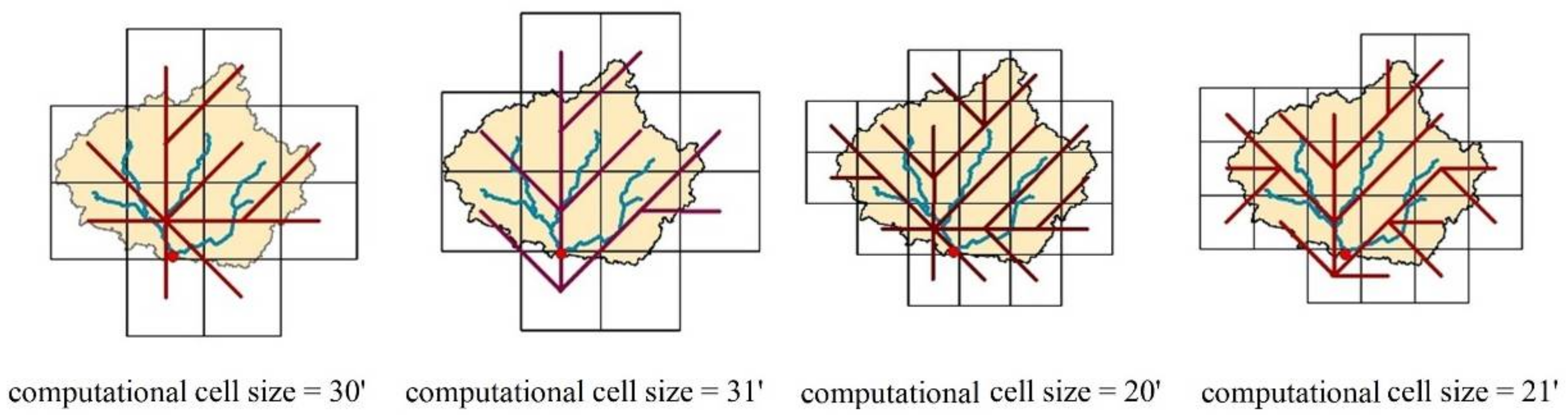
The performance of the LRR routing method is, however, different from that of the I-NRF routing method, as it fluctuates as the computational cell size changes (Figure 4c,d Figure 5c,d and Figure 6c,d). The PBAIS shows the same trend as NSE. The computational cell size affects the LRR PBAIS more than I-NRF PBIAS. Furthermore, the fluctuations observed in the NSE values in the Jianxi and Shizhenjie basins are not identical. For Jianxi basin, the NSE curve fluctuates greatly, from 20′ to 21′ and from 30′ to 31′, etc., for every DEM resolution (Figure 4 and Figure 6). For the Shizhenjie basin, the NSE curve fluctuates from 18′ to 19′ and from 28′ to 29′, etc., with DEM of 90 m. It fluctuates greatly from 19′ to 20′ and from 28′ to 29′, etc., with DEM of 250 m, 500 m and 1000 m (Figure 5 and Figure 6).
The sensitivity of the LRR routing method to the computational cell size arises because the flow net changes with the computational cell size [18]. In fact, the flow net experiences distinct structural changes as the computational cell size changes. For example, the NSE curve fluctuates greatly, from 20′ to 21′ and from 30′ to 31′, etc., for every DEM resolution in Jianxi basin (Figure 4 and Figure 6). The differences of computational cell size between 20′ and 21′ or 30′ and 31′ are very small, but the resulting NSE differences are significant. To better understand these turning points, the extracted river networks for computational cell sizes of 20′, 21′, 30′, and 31′ in the Jianxi basin are plotted in Figure 7. From 20′ to 21′ and from 30′ to 31′, minor changes in the computational cell size lead to a different allocation of the outlet grid cells, which ultimately results in a significant difference in the flow net. Besides, the LRR routing method is based on the flow net at a given computational cell size. As such, a small change in the computational cell size leads to a large difference in the NSE value.
Additionally, the LRR NSE values are also sensitive to the computational cell size because smaller computational cell sizes correspond to a finer and different flow net (Figure 3). The high-resolution flow net not only better captures the shape of the real river network, but also better simulates the length of the routing path. In the LRR method, the length of the routing path affects the deformation and the smoothing of the flood. A coarser computational cell size reduces the flow net between cells into a straight line, which explains why the NSE value is higher and PBIAS is smaller when the computational cell size is small. The result that the LRR routing method is sensitive to the computational cell size confirmed the result from Arora et al. [45]. In that study, a finer computational cell size resulted in better performance.
Whether the NSE of the LRR and I-NRF routing method is sensitive to computational cell size is not related to the runoff generation model and the specific study basin in this study, indicating that this pattern is universal. Therefore, to accurately simulate the discharge, larger computational cell sizes can be used to save computing time when the I-NRF routing method is used. For the LRR routing method, however, the choice of computational cell size must be an informed decision.
4.2. The Effect of the DEM Resolution on the Discharge Simulation Performance
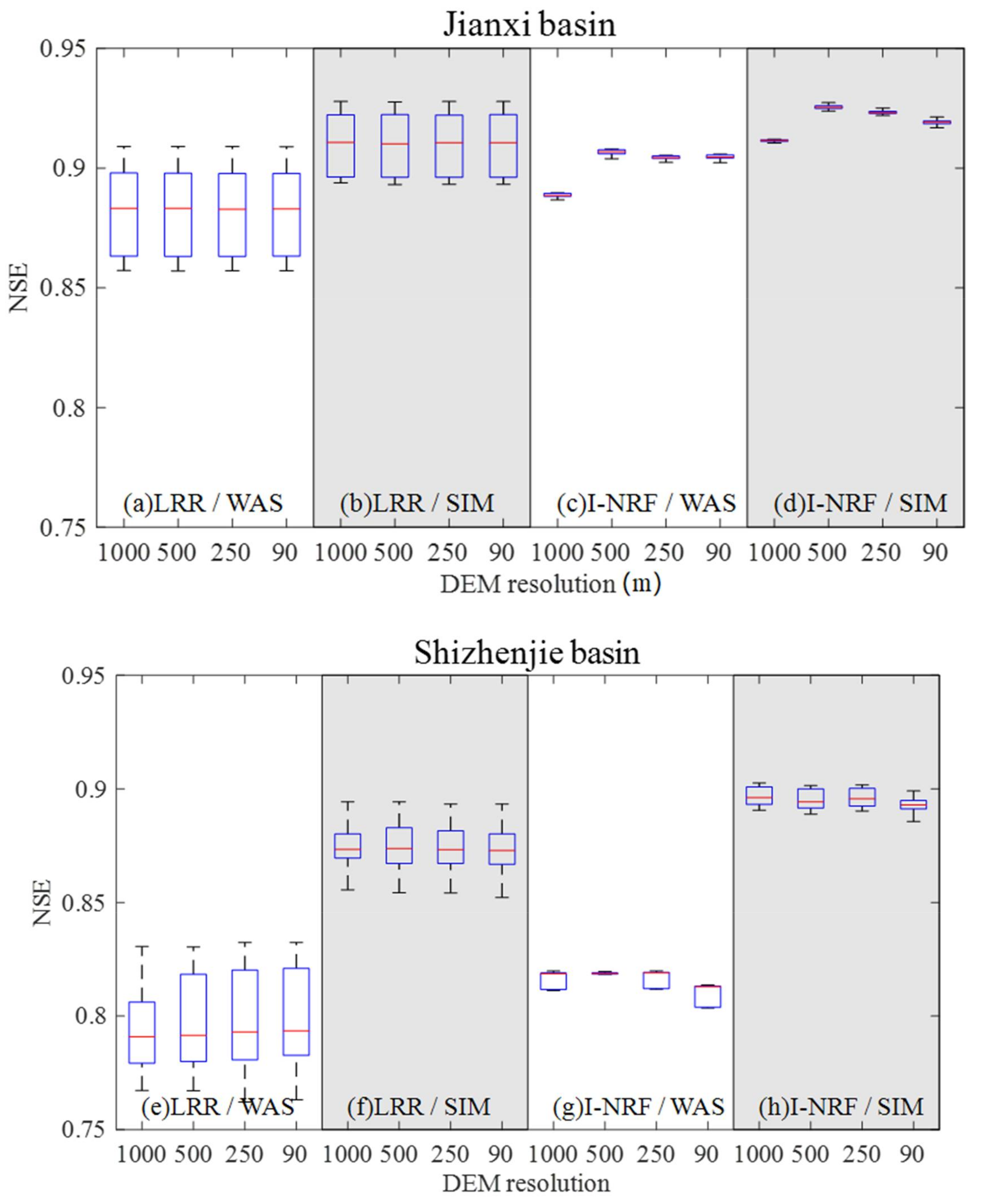
Box plots of NSE value variations with the computational cell size and the DEM resolution are shown in Figure 8. The impact of the DEM resolution on the discharge simulation performance is slightly larger for the I-NRF routing method than it is for the LRR routing method. For the I-NRF routing method, the use of different DEM resolutions leads to some differences in modelling performance, for both runoff generation models and for both study basins; from these observations, it can be inferred that the DEM resolution directly affects the NSE values, to some extent (Figure 8c,d,g,h). For the LRR routing method, the average NSE for all computational cell sizes is similar when DEM resolution changes, regardless of the runoff generation model or the study basin. As such, it can be concluded that the DEM resolution has little effect on the overall LRR discharge simulation performance (Figure 8a,b,e,f). The laws analyzed from changes in PBIAS are the same as those analyzed from changes in NSE.
With the I-NRF routing method, different DEM resolutions produce variations in the overall discharge simulation performance (Figure 6 and Figure 8). However, in this study, the difference in the NSE values generated by the different DEM resolutions is less than 0.03 (Figure 6), while the difference in the NSE values due to the implementation of the two runoff generation models is greater than 0.03 (Figure 6). Besides, as shown in Figure 8, there is no consistent correlation between the DEM resolution and the overall discharge simulation performance for the I-NRF routing method. In the I-NRF routing method, an accurate simulation of discharge value requires an accurate simulation of the routing time. As per Equation (1), the routing time is calculated using the slope and the routing length. The slope and routing length both increase with a finer DEM resolution [46]. In practice, it is difficult to predict whether the value is closer to or further from the true routing time value when the DEM resolution becomes finer (Equation (1)). Consequently, a finer DEM resolution does not necessarily correspond to higher NSE values, a fact that was observed in our study. In the Jianxi basin, the worst discharge simulation is generated with a DEM resolution of 1000 m 1000 m; in the Shizhenjie basin, the worst discharge simulation is generated with a DEM resolution of 90 m × 90 m. Figure 3, Figure 4 and Figure 6 also show that DEM resolution and computational cell size have almost no joint influence on the result of I-NRF.
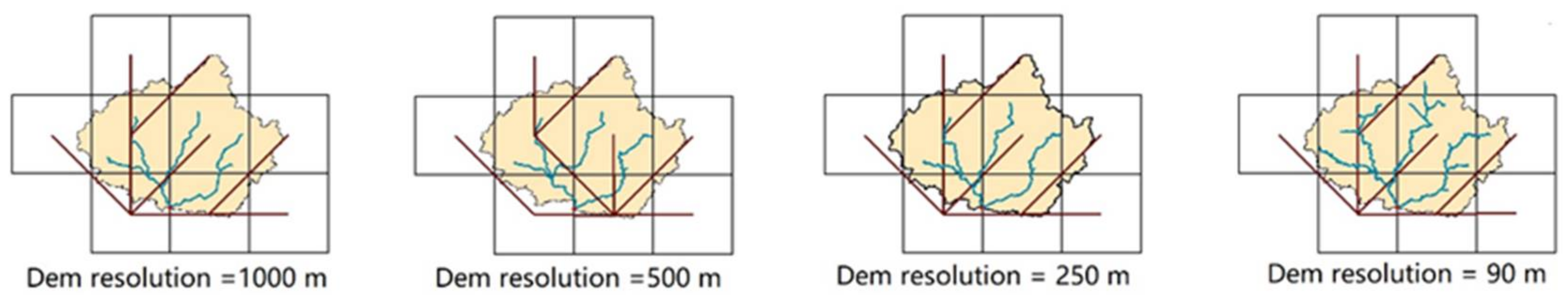
For the LRR routing method, the NSE difference introduced by DEM resolution is much smaller than that of computational cell size (Figure 6 and Figure 8a,b,e,f). Finer DEM resolution does not result in better model performance (Figure 8a,b,e,f). As discussed previously, the LRR routing method is based on the flow net at a given computational cell size. In addition, even the coarsest DEM resolution (1000 m) is still much smaller than the smallest computational cell size (about 8180 m). Thus, the DEM slope and routing length are largely irrelevant. Combining Figure 8 with Figure 6, it can be seen that the NSE with a DEM resolution of 500 m is different from others at the computational cell size of 26′ and 39′ in the Jianxi basin. Furthermore, for the Shizhenjie watershed, the NSE curves corresponding to each DEM resolution do not overlap. To understand the difference caused by the DEM resolution, the flow nets at the computational cell size of 39′ with DEM resolutions of 1000 m, 500 m, 250 m, 90 m in the Jianxi basin are drawn in Figure 9. It can be seen that the flow net with the DEM resolution of 500 m is different from the others. That is the reason why NSE with the DEM resolution of 500 m is different from others at the computational cell sizes of 39′. Now it is known that the DEM resolution and the computational cell size affect the upscaled flow net at the same time. On the one hand, when the DEM resolution is different, the flow direction identification of some computational cells may be different, which will cause disturbance to the basin flow net. On the other hand, the computational cell size will also affect the basin flow net, as described in Section 4.1. Because the flow net directly affects the discharge simulation performance in the LRR routing method, it can be proposed that the DEM resolution and the computational cell size jointly affect the simulated discharge when the LRR routing method is implemented. However, the joint effect is very small and can be ignored in the actual simulation (Figure 6 and Figure 8).
In this paper, both coarser and finer DEMs are sufficient for hydrological modelling with those conceptual models. However, such conclusions are not suitable for most hydraulic models. When using a hydrodynamic model, caution is still required regarding the choice of DEM resolution. For example, Horrit et al. [71] studied the effect of DEM resolution on the LISFLOOD-FP model, using a 1D description of channel flow. Models with resolutions varying from 10 to 1000 m are compared. The results showed that the model achieves the best simulation of the inundated area when using a 100 m DEM. Cook and Merwade [72] found that using a 1D HEC-RAS model, and a 2D FESWMS model, the flood inundation area reduces with improved horizontal resolution and vertical accuracy in the topographic model.
In order to facilitate researchers to choose the appropriate routing method when conducting hydrological simulations, this paper lists the time duration of the two models. Taking the case of using the WASMOD runoff generation model and Jianxi basin as an example, the running times of the two routing methods are compared (Table 6). According to the above discussion, for both routing methods, a finer DEM cannot guarantee a better simulation effect. Therefore, the time duration of the model under different DEM resolutions is not discussed here. It should be noted that the time duration of the models listed in this article does not include pre-processing and preparation of data, but includes parameter optimization of the model. The computer used to count the running time is as follows. OS: Windows 10 Pro 64-bit; CPU: Intel Core i7-9700 @ 3.00GHz eight-core; Memory: 16 GB; Sofeware: MATLAB R2020b.
It can be seen that the time duration of both routing methods is within the acceptable range, and the time duration of I-NRF is slightly shorter. However, a finer computational cell size leads to a huge increase in time duration. Thus, a finer computational cell size means a longer time duration and better simulation performance for the LRR routing method, while coarser computational cell size can be used with the I-NRF routing method to save time. Therefore, this paper proposes to choose the I-NRF routing model when conducting watershed-scale hydrological simulations.
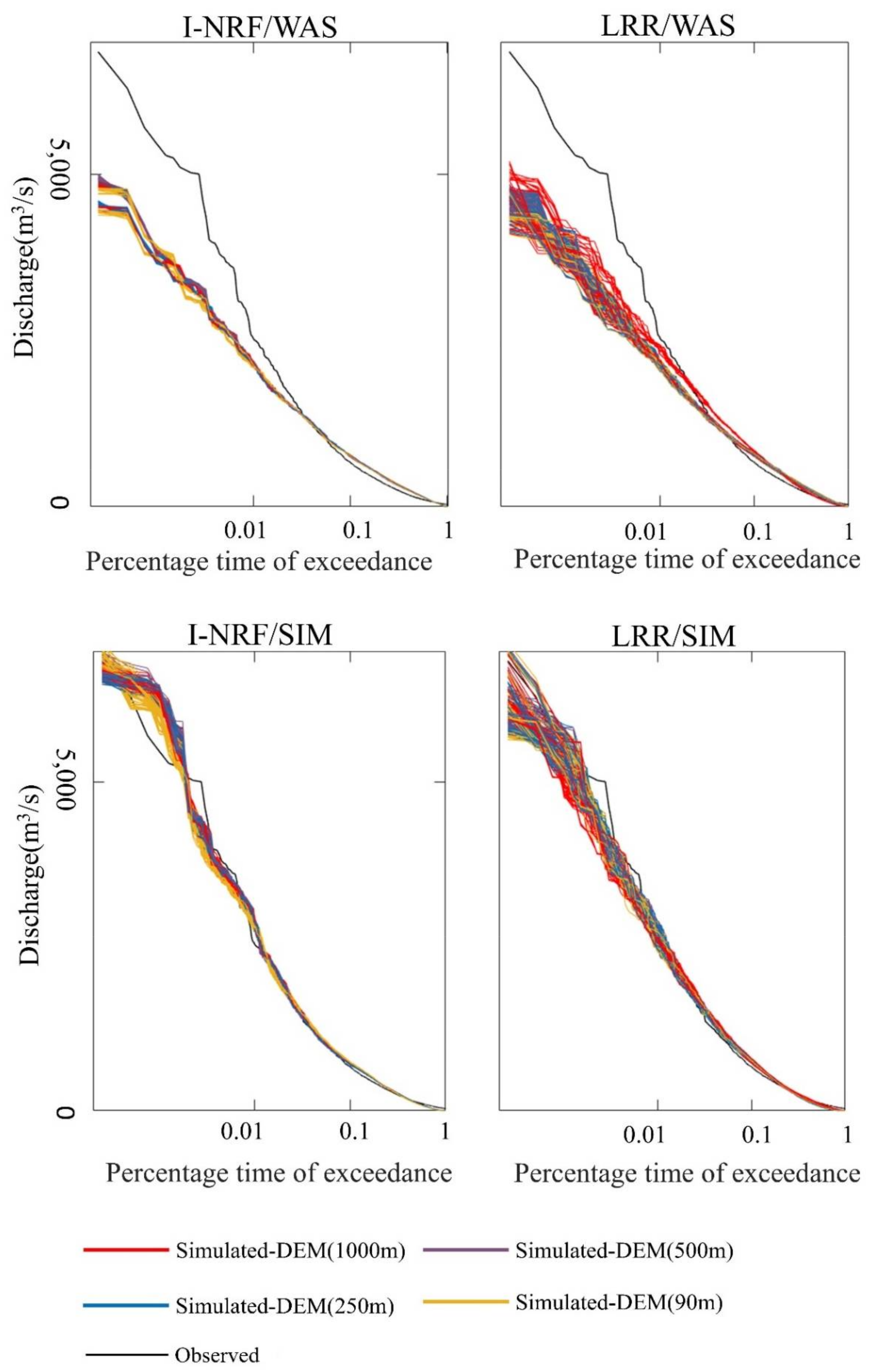
4.3. Analysis of Discharge Duration Curves
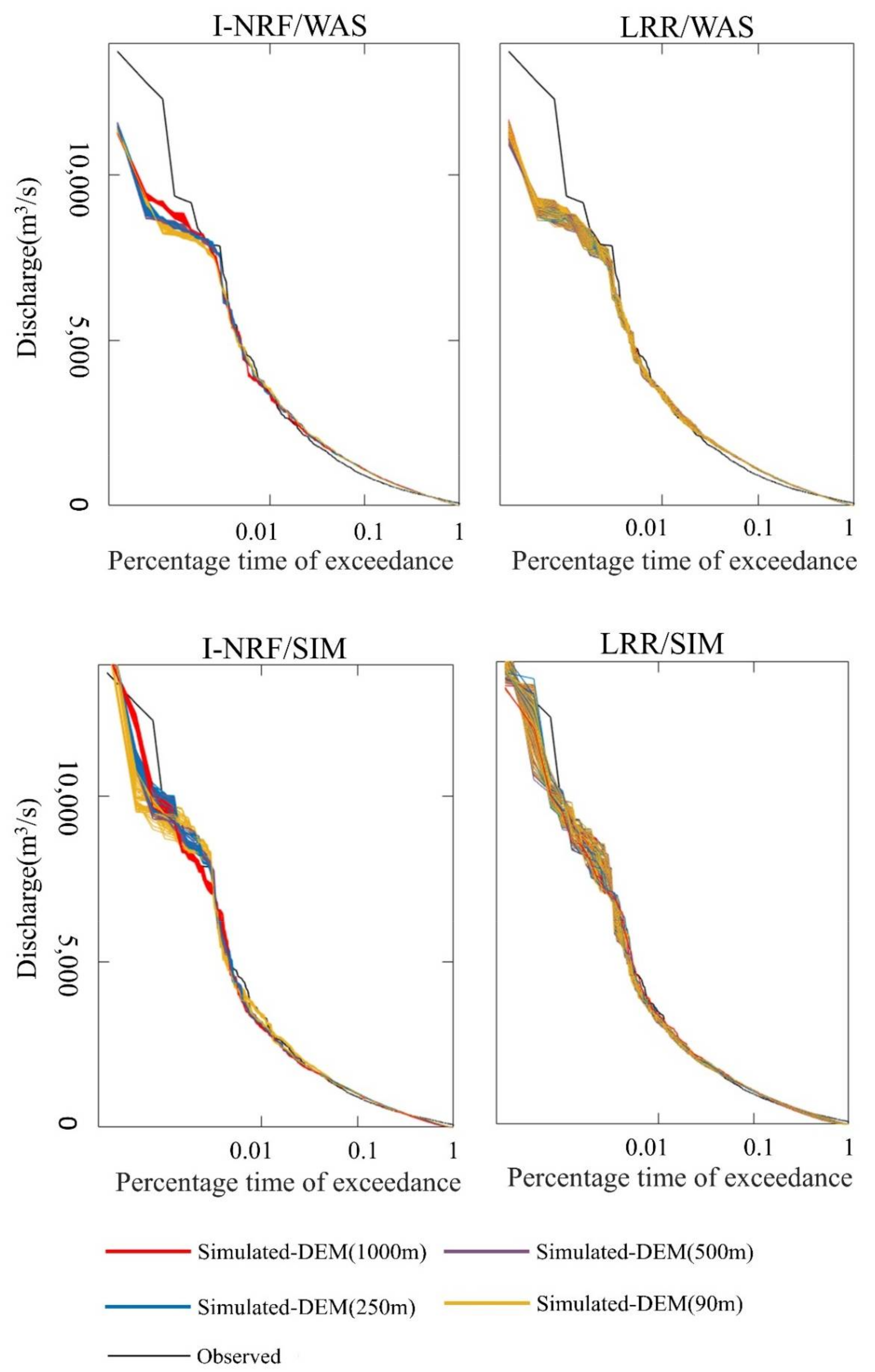
To further analyze the effects of the DEM resolution and the computational cell size on the simulated discharge for the two routing methods, the corresponding discharge duration curves are calculated for each DEM resolution and computational cell size. The discharge duration curve is a statistical curve that represents the proportion of days in which the flow exceeds a specified threshold value in a certain time period. Figure 10 and Figure 11 plot the observed discharge duration curve and the simulated discharge duration curve clusters for the various DEM resolutions and computational cell sizes. The colors of the simulated discharge duration curve clusters correspond to the different DEM resolutions. The ordinate is the daily flow and the abscissa is the cumulative proportion. To more easily visualize the instances of high flow predicted by the hydrological models, a horizontal logarithmic axis is applied to this plot. Smaller values on the horizontal axis correspond to larger flows.
As shown in Figure 10 and Figure 11, both DEM resolutions and computational cell size influence the simulated discharge. The effects of the computational cell size and the DEM resolution on the simulated discharge accuracy are mainly reflected in the high-flow range (i.e., the first 1% of the discharge). As shown by the discharge duration curves of the two runoff generation methods, it can be seen that the WASMOD model tends to underestimate the high flow, and SIMHYD can simulate high flow better than WASMOD in the study area.
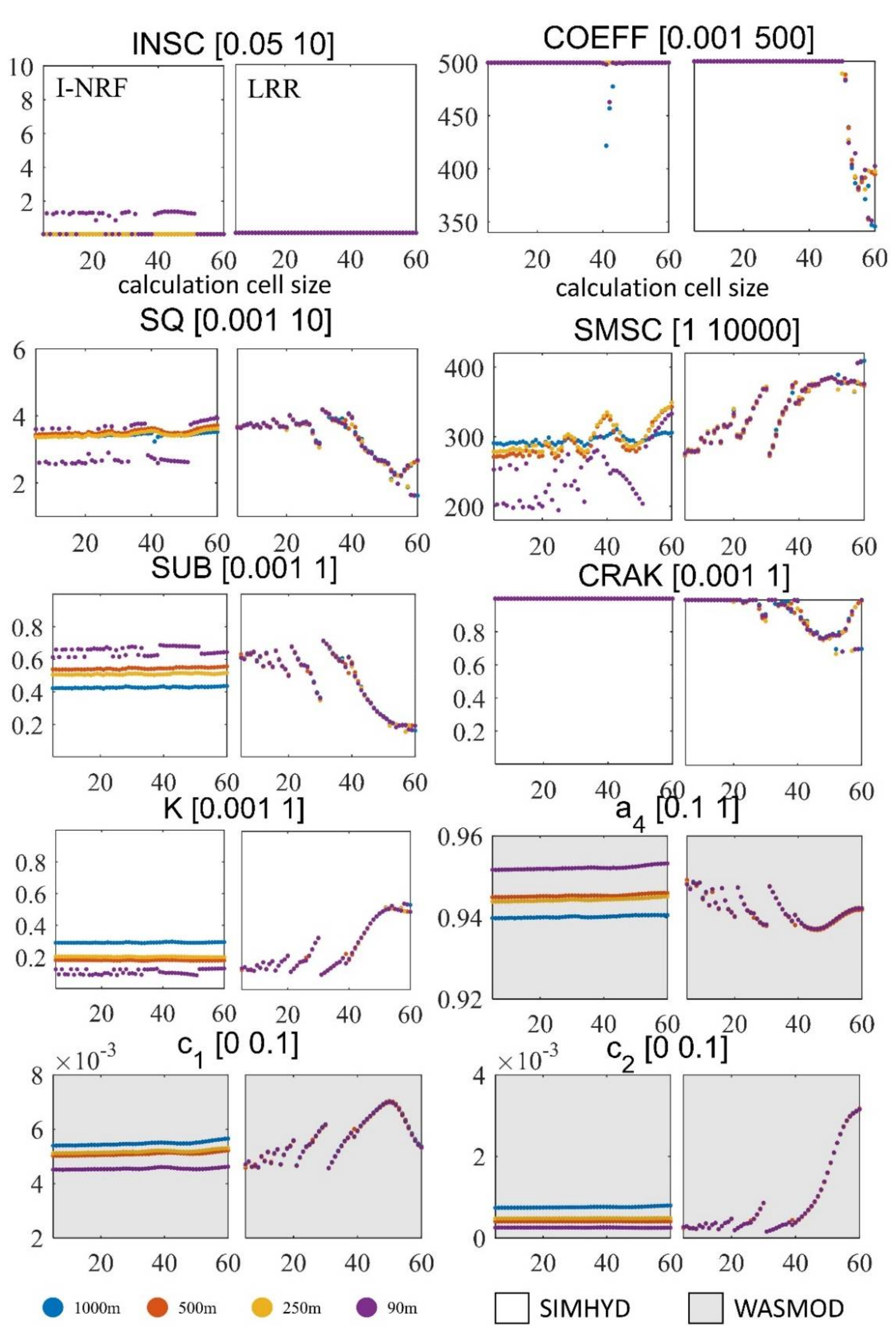
4.4. Analysis of Runoff Generation Parameters
The optimal runoff generation parameters in the Jianxi and Shizhenjie basins, identified from a combination of 4 DEM resolutions and 56 computational cell sizes, are shown in Figure 12 and Figure 13.
In the Jianxi basin, the optimal runoff generation parameters with the I-NRF routing method vary with the different DEM resolutions (Figure 12). Furthermore, when the runoff generation parameters with the I-NRF routing method change with the computational cell size, parameters , , and in the WASMOD model are more stable than the parameters in the SIMHYD model, a difference that may be caused by the equifinality effect that arises due to the higher number of parameters in the SIMHYD model. The equifinality of model parameter sets is a common phenomenon. There are records of this phenomenon in Beven [73,74]. The optimal runoff generation parameters with the LRR routing method appear to be largely insensitive to the DEM resolution. With the LRR routing method, the turning points in the curves in Figure 12 correspond somewhat to those in Figure 6c. Additionally, they show the same or the opposite trend to the NSE curves. Some parameters are sensitive to the computational cell size, while others are not. In the Jianxi basin, parameters SUSC, K, , and exhibit opposing NSE trends. While, parameters SQ, SMSC, SUB, and K in the SIMHYD model and parameters , , and in the WASMOD model, parameters , SUB, and SQ, exhibit similar trends with NSE (Figure 12 and Figure 6c).
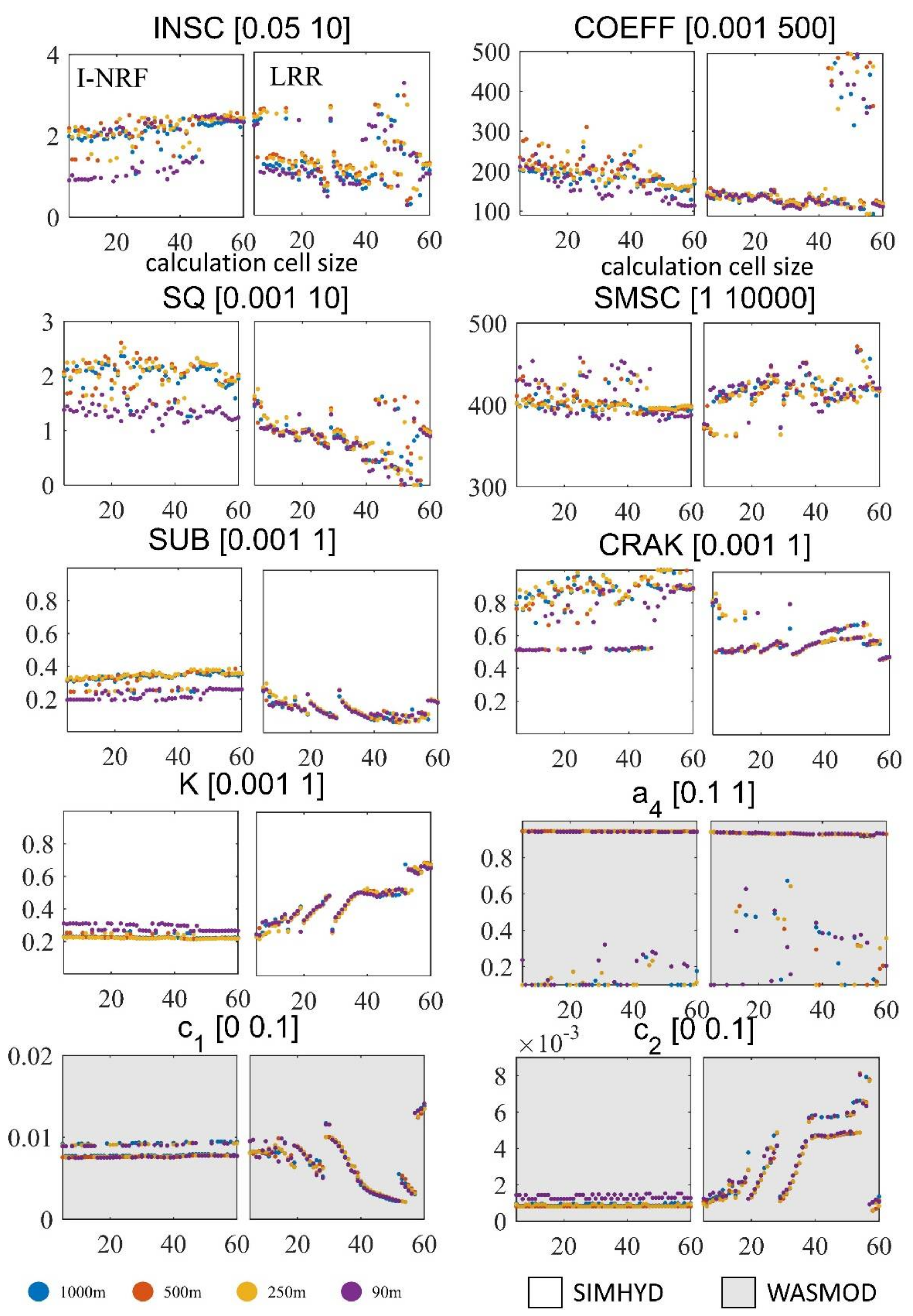
The results for the Shizhenjie basin are shown in Figure 13. Just as they did in the Jianxi basin, the optimal runoff generation parameters with the I-NRF routing method vary with the DEM resolutions. The runoff generation parameters with the I-NRF routing method vary much more widely with the computational cell size in the Shizhenjie basin than they do in the Jianxi basin. Besides, the runoff generation parameters with the LRR routing method vary much more widely with the DEM resolutions in the Shizhenjie basin than they do in the Jianxi basin. With the LRR routing method, the parameters and SUB follow the same NSE trends, while parameters K and exhibit opposing NSE trends as computational cell size changes in the Shizhenjie basin (Figure 13 and Figure 6d).
5. Conclusions
Previous studies have reported how the DEM resolution and computational cell size affect the modelling results separately. However, too little work has been devoted to how they jointly affect the routing method performance. This study sought to understand how the DEM resolution and the computational cell size jointly affect the simulated discharge results produced by the I-NRF and LRR routing methods. Two runoff-generation models were used to test the generality of the result. In these models, computational cell sizes that range from 5 arc-min to 60 arc-min, with an interval of 1 arc-min and DEM resolutions of 90 m, 250 m, 500 m, and 1000 m are used. The conclusions are as follows:
- 1.
- The DEM resolution has a larger impact on the I-NRF discharge simulation performance than it does for the LRR method. However, the overall I-NRF discharge simulation performance is not consistently correlated with DEM resolution. As the computational cell size increases, the I-NRF discharge simulation performance is relatively stable because the I-NRF method is largely independent of the computational cell size. The DEM resolution and the computational cell size exert no joint influence on the I-NRF discharge simulation performance.
- 2.
- The DEM resolution has little effect on the LRR discharge simulation performance. The LRR discharge simulation performance changes drastically with the computational cell size for both runoff generation models. In general, finer computational cell size leads to better results, while the LRR discharge simulation performance oscillates heavily as the computational cell size increases. The joint effect of DEM resolution and the computational cell size on the performance of the LRR routing method can be ignored in hydrological modelling.
- 3.
- The effects of the computational cell size and the DEM resolution on the simulated discharge accuracy are mainly reflected in the high-flow range. In this study, the performance of SIMHYD is better than that of WASMOD in the high-flow range, when they are combined with both routing methods.
These results will provide guidance as to how hydrological researchers can use their knowledge of the study area and their computational limitations to make reasonable routing method, DEM resolution, and computational cell size choices.
Author Contributions
Conceptualization, J.L.; methodology, J.L.; software, J.L., H.Z. and L.L.; validation, J.L., and R.H.; formal analysis, J.L.; investigation, J.L.; resources, J.L.; data curation, J.L.; writing—original draft preparation, J.L.; writing—review and editing, H.C., L.L., J.C. and C.-Y.X.; visualization, R.H.; supervision, H.C. and C.-Y.X.; project administration, H.C.; funding acquisition, C.-Y.X. All authors have read and agreed to the published version of the manuscript.
Funding
This study was partly supported by the National Key Research and Development Program (2017YFA0603702), and the Research Council of Norway (FRINATEK Project 274310). The APC was funded by the National Key Research and Development Program (2017YFA0603702).
Data Availability Statement
The DEM with the resolution of 1000 m is obtained from https://www.usgs.gov/centres/eros/science/usgs-eros-archive-digital-elevation-hydro1k?qt-science_centre_objects=0#qt-science_centre_objects (accessed on 14 January 2022). The DEM with the resolution of 500 m, 250 m and 90 m are all available at http://www.resdc.cn/data.aspx?DATAID=123 (accessed on 14 January 2022). The discharge data used in this study are not provided due to the confidentiality of the data. The daily precipitation, air temperature, and relative humidity data are available at http://data.cma.cn/ (accessed on 14 January 2022).
Conflicts of Interest
The authors declare no conflict of interest. The funders had no role in the design of the study; in the collection, analyses, or interpretation of data; in the writing of the manuscript, or in the decision to publish the results.
References
- Gao, L.; Tao, B.; Miao, Y.; Zhang, L.; Xu, X. A global dataset for economic losses of extreme hydrological events during 1960–2014. Water Resour. Res. 2019, 55, 5165–5175. [Google Scholar] [CrossRef]
- Funk, C.; Shukla, S.; Thiaw, W.M.; Rowland, J.; Hoell, A.; McNally, A.; Husak, G.; Novella, N.; Budde, M.; Peters-Lidard, C. Recognizing the Famine Early Warning Systems Network: Over 30 Years of Drought Early Warning Science Advances and Partnerships Promoting Global Food Security. Bull. Am. Meteorol. Soc. 2019, 100, 1011–1027. [Google Scholar] [CrossRef]
- Abnakorn, S.; Ruangpan, L.; Tangdamrongsub, N.; Suryadi, F.X.; Fraiture, C.D. Improving flood and drought management in agricultural river basins: An application to the Mun River Basin in Thailand. Water Policy 2021, 23, 1153–1169. [Google Scholar] [CrossRef]
- Lu, E.; Luo, Y.; Zhang, R.; Wu, Q.; Liu, L. Regional atmospheric anomalies responsible for the 2009–2010 severe drought in China. J. Geophys. Res. Atmos. 2011, 116, D21114. [Google Scholar] [CrossRef]
- Nyandiko, N.O. Devolution and Disaster Risk Reduction in Kenya: Progress, challenges and opportunities. Int. J. Disast. Risk Reduct. 2020, 51, 101832. [Google Scholar] [CrossRef]
- Bruno, M.; Florian, E.; Michael, K.; Bernhard, M.; Schröter, K.; Steffi, U.-E. The extreme flood in June 2013 in Germany. La Houille Blanche 2014, 1, 5–10. [Google Scholar]
- Ulbrich, U.; Brücher, T.; Fink, A.H.; Leckebusch, G.C.; Krüger, A.; Pinto, J.G. The central European floods of August 2002: Part 1—Rainfall periods and flood development. Weather 2003, 58, 371–377. [Google Scholar] [CrossRef] [Green Version]
- Lal, P.; Prakash, A.; Kumar, A.; Srivastava, P.K.; Khan, M.L. Evaluating the 2018 extreme flood hazard events in Kerala, India. Remote Sens. Lett. 2020, 11, 436–445. [Google Scholar] [CrossRef]
- Wang, Y.; Xu, Y.; Lei, C.; Li, G.; Han, L.; Song, S.; Yang, L.; Deng, X. Spatio-temporal characteristics of precipitation and dryness/wetness in Yangtze River Delta, eastern China, during 1960–2012. Atmos. Res. 2016, 172–173, 196–205. [Google Scholar] [CrossRef]
- Denić, N.; Petković, D.; Spasic, B. Global Economy Increasing by Enterprise Resource Planning. In Reference Module in Materials Science and Materials Engineering; Elsevier Inc.: London, UK, 2020; pp. 331–337. [Google Scholar]
- Denić, N.; Petković, D.; Siljkovi, B.; Ivkovi, R. Opportunities for Digital Marketing in the Viticulture of Kosovo and Metohija. In Reference Module in Materials Science and Materials Engineering; Elsevier Inc.: London, UK, 2020. [Google Scholar]
- Petkovic, D.; Petković, B.; Kuzman, B. Appraisal of information system for evaluation of kinetic parameters of biomass oxidation. Biomass-Convers. Biorefinery 2020, 10, 1–9. [Google Scholar] [CrossRef]
- Lakovic, N.; Khan, A.; Petković, B.; Petkovic, D.; Kuzman, B.; Resic, S.; Jermsittiparsert, K.; Azam, S. Management of higher heating value sensitivity of biomass by hybrid learning technique. Biomass Convers. Biorefinery 2021, 1–8. [Google Scholar] [CrossRef]
- Mili, M.; Petkovi, B.; Selmi, A.; Petkovi, D.; Kuzman, B. Computational evaluation of microalgae biomass conversion to biodiesel. Biomass Convers. Biorefin. 2021, 11, 1–8. [Google Scholar] [CrossRef]
- Milićević, V.; Denić, N.; Milićević, Z.; Arsić, L.; Spasić-Stojković, M.; Petković, D.; Stojanović, J.; Krkic, M.; Milovančević, N.S.; Jovanović, A. E-learning perspectives in higher education institutions. Technol. Forecast. Soc. Chang. 2021, 166, 120618. [Google Scholar] [CrossRef]
- Spasi, B.; Siljkovi, B.; Deni, N.; Petkovi, D.; Vujovi, V. Natural Lignite Resources in Kosovo and Metohija and Their Influence on the Environment. Min. Metall. Eng. Bor 2020, 1, 561–566. [Google Scholar]
- Kuzman, B.; Petkovi, B.; Denić, N.; Petkovi, D.; Momir, M. Estimation of optimal fertilizers for optimal crop yield by adaptive neuro fuzzy logic. Rhizosphere 2021, 18, 100358. [Google Scholar] [CrossRef]
- Gong, L.; Widen-Nilsson, E.; Halldin, S.; Xu, C.-Y. Large-scale runoff routing with an aggregated network-response function. J. Hydrol. 2009, 368, 237–250. [Google Scholar] [CrossRef]
- Papaioannou, G.; Loukas, A.; Vasiliades, L.; Aronica, G.T. Sensitivity analysis of a probabilistic flood inundation mapping framework for ungauged catchments. Water 2017, 60, 9–16. [Google Scholar]
- Bellos, V.; Kourtis, I.M.; Moreno-Rodenas, A.; Tsihrintzis, V.A. Quantifying Roughness Coefficient Uncertainty in Urban Flooding Simulations through a Simplified Methodology. Water 2017, 9, 944. [Google Scholar] [CrossRef] [Green Version]
- Hui, J.; Wu, Y.; Zhao, F.; Lei, X.; Li, J. Parameter Optimization for Uncertainty Reduction and Simulation Improvement of Hydrological Modeling. Remote Sens. 2020, 12, 4069. [Google Scholar] [CrossRef]
- Pappenberger, F.; Matgen, P.; Beven, K.J.; Henry, J.B.; Pfister, L.; De, P.F. Influence of uncertain boundary conditions and model structure on flood inundation predictions. Adv. Water Resour. 2006, 29, 1430–1449. [Google Scholar] [CrossRef]
- Samela, C.; Manfreda, S.; Paola, F.D.; Giugni, M.; Fiorentino, M. DEM-Based Approaches for the Delineation of Flood-Prone Areas in an Ungauged Basin in Africa. J. Hydrol. Eng. 2016, 21, 06015010. [Google Scholar] [CrossRef]
- Teng, J.; Jakeman, A.J.; Vaze, J.; Croke, B.; Dutta, D.; Kim, S. Flood inundation modelling: A review of methods, recent advances and uncertainty analysis. Environ. Modell. Softw. 2017, 90, 201–216. [Google Scholar] [CrossRef]
- Rozos, E.; Dimitriadis, P.; Bellos, V. Machine Learning in Assessing the Performance of Hydrological Models. Hydrology 2022, 9, 5. [Google Scholar] [CrossRef]
- Wang, M.; Hjelmfelt, A.T. DEM Based Overland Flow Routing Model. J. Hydrol. Eng. 1998, 3, 1–8. [Google Scholar] [CrossRef]
- Bates, P.D.; Roo, A. A simple raster-based model for flood inundation simulation. J. Hydrol. 2000, 236, 54–77. [Google Scholar] [CrossRef]
- Bellos, V.; Tsakiris, G. A hybrid method for flood simulation in small catchments combining hydrodynamic and hydrological techniques. J. Hydrol. 2016, 540, 331–339. [Google Scholar] [CrossRef]
- Li, H.; Beldring, S.; Xu, C.-Y. Implementation and testing of routing algorithms in the distributed Hydrologiska Byråns Vattenbalansavdelning model for mountainous catchments. Hydrol. Res. 2014, 45, 322–333. [Google Scholar] [CrossRef] [Green Version]
- Olivera, F.; Famiglietti, J.; Asante, K. Global-scale flow routing using a source-to-sink algorithm. Water Resour. Res. 2000, 36, 2197–2207. [Google Scholar] [CrossRef]
- Arora, V.K.; Boer, G.J. A variable velocity flow routing algorithm for GCMs. J. Geophys. Res.-Atmos. 1999, 104, 30965–30979. [Google Scholar] [CrossRef]
- Huang, P.C.; Lee, K.T. Efficient DEM-based overland flow routing using integrated recursive algorithms. Hydrol. Process. 2017, 31, 1007–1017. [Google Scholar] [CrossRef]
- Sausen, R.; Schubert, S.; Dümenil, L. A model of river runoff for use in coupled atmosphere-ocean models. J. Hydrol. 1994, 155, 337–352. [Google Scholar] [CrossRef]
- Miller, J.R.; Russell, G.L.; Caliri, G. Continental-scale river flow in climate models. J. Clim. 1994, 7, 914–928. [Google Scholar] [CrossRef] [Green Version]
- Gong, L.; Halldin, S.; Xu, C.-Y. Global-scale river routing—An efficient time-delay algorithm based on HydroSHEDS high-resolution hydrography. Hydrol. Process. 2011, 25, 1114–1128. [Google Scholar] [CrossRef]
- Lu, G.; Liu, J.; Wu, Z.; Hai, H.; Xu, H.; Lin, Q. Development of a Large-Scale Routing Model with Scale Independent by Considering the Damping Effect of Sub-Basins. Water Resour. Manag. 2015, 29, 5237–5253. [Google Scholar] [CrossRef]
- Ducharne, A.; Golaz, C.; Leblois, E.; Laval, K.; Polcher, J.; Ledoux, E.; de Marsily, G. Development of a high resolution runoff routing model, calibration and application to assess runoff from the LMD GCM. J. Hydrol. 2003, 280, 207–228. [Google Scholar] [CrossRef]
- Harrigan, S.; Zsoter, E.; Alfieri, L.; Prudhomme, C.; Pappenberger, F. GloFAS-ERA5 operational global river discharge reanalysis 1979-present. Earth Syst. Sci. Data 2020, 12, 2043–2060. [Google Scholar] [CrossRef]
- Van Der Knijff, J.M.; Younis, J.; De Roo, A.P.J. LISFLOOD: A GIS-based distributed model for river basin scale water balance and flood simulation. Int. J. Geogr. Inf. Sci. 2010, 24, 189–212. [Google Scholar] [CrossRef]
- Hersbach, H.; Rosnay, P.; Bell, B.; Schepers, D. Operational Global Reanalysis: Progress, Future Directions and Synergies with NWP; European Centre for Medium Range Weather Forecasts: Reading, UK, 2018. [Google Scholar]
- Xie, Z.; Yuan, F.; Duan, Q.; Zheng, J.; Liang, M.; Chen, F. Regional parameter estimation of the VIC land surface model: Methodology and application to river basins in China. J. Hydrometeorol. 2007, 8, 447–468. [Google Scholar] [CrossRef] [Green Version]
- Niu, J.; Chen, J.; Wang, K.; Sivakumar, B. Multi-scale streamflow variability responses to precipitation over the headwater catchments in southern China. J. Hydrol. 2017, 551, 14–28. [Google Scholar] [CrossRef]
- Avand, M.; Kuriqi, A.; Khazaei, M.; Ghorbanzadeh, O. DEM resolution effects on machine learning performance for flood probability mapping. J. Hydro-Environ. Res. 2022, 40, 1–16. [Google Scholar] [CrossRef]
- Du, J.; Xie, H.; Hu, Y.; Xu, Y.; Xu, C.-Y. Development and testing of a new storm runoff routing approach based on time variant spatially distributed travel time method. J. Hydrol. 2009, 369, 44–54. [Google Scholar] [CrossRef]
- Arora, V.; Seglenieks, F.; Kouwen, N.; Soulis, E. Scaling aspects of river flow routing. Hydrol. Process 2001, 15, 461–477. [Google Scholar] [CrossRef]
- Song, X.; Qi, Z.; Du, L.P.; Kou, C.L. The Influence of DEM Resolution on Hydrological Simulation in the Huangshui River Basin. Int. J. Geogr. Inf. Sci. 2012, 518, 4299–4302. [Google Scholar] [CrossRef]
- Jeon, J.H.; Ham, J.H.; Yoon, C.G.; Kim, S.J. Effects of DEM Resolution on Hydrological Simulation in, BASINS-BSPF Modeling. Mag. Korean Soc. Agric. Eng. 2002, 44, 25–35. [Google Scholar]
- Chaubey, I.; Cotter, A.S.; Costello, T.A.; Soerens, T.S. Effect of DEM data resolution on SWAT output uncertainty. Hydrol. Process. 2005, 19, 621–628. [Google Scholar] [CrossRef] [Green Version]
- Li, J.; Zhao, H.; Zhang, J.; Chen, H.; Xu, C.; Li, L.; Chen, J.; Guo, S. An improved routing algorithm for a large scale distributed hydrological model with consideration of underlying surface impact. Hydrol. Res. 2020, 51, 834–852. [Google Scholar] [CrossRef]
- USGS HYDRO1k Elevation Derivative Database. Available online: https://www.usgs.gov/centers/eros/science/usgs-eros-archive-digital-elevation-hydro1k?qt-science_center_objects=0#qt-science_center_objects (accessed on 14 January 2022).
- Dimitriadis, P.; Koutsoyiannis, D.; Iliopoulou, T.; Papanicolaou, P. A Global-Scale Investigation of Stochastic Similarities in Marginal Distribution and Dependence Structure of Key Hydrological-Cycle Processes. Hydrology 2021, 8, 59. [Google Scholar] [CrossRef]
- Courant, R.; Friedrichs, K.; Lewy, H. On the partial difference equations of mathematical physics. IBM J. Res. Dev. 1967, 11, 215–234. [Google Scholar] [CrossRef]
- Chiew, F.H.S.; Peel, M.C.; Western, A.W.; Singh, V.P.; Frevert, D. Application and testing of the simple rainfall-runoff model SIMHYD. In Mathematical Models of Small Watershed Hydrology and Applications; Water Resources Publication: Highlands Ranch, CO, USA, 2002. [Google Scholar]
- Wang, J.; Wang, G.; Elmahdi, A.; Bao, Z.; Song, M. Comparison of hydrological model ensemble forecasting based on multiple members and ensemble methods. Open Geosci. 2021, 13, 401–415. [Google Scholar] [CrossRef]
- Chiew, F.H.S.; Teng, J.; Vaze, J.; Post, D.A.; Perraud, J.M.; Kirono, D.G.; Viney, N.R. Estimating climate change impact on runoff across southeast Australia: Method, results, and implications of the modeling method. Water Resour. Res. 2009, 45, 82–90. [Google Scholar] [CrossRef]
- Li, H.; Zhang, Y. Regionalising rainfall-runoff modelling for predicting daily runoff: Comparing gridded spatial proximity and gridded integrated similarity approaches against their lumped counterparts. J. Hydrol. 2017, 550, 279–293. [Google Scholar] [CrossRef]
- Liang, K.; Liu, C.; Liu, X.; Song, X. Impacts of climate variability and human activity on streamflow decrease in a sediment concentrated region in the Middle Yellow River. Stoch. Env. Res. A 2013, 27, 1741–1749. [Google Scholar] [CrossRef]
- Xu, C.Y. WASMOD—The water and snow balance modeling system. In Mathematical Models of Small Watershed Hydrology Applications; Singh, V.P., Frevert, D., Eds.; Water Resources Publication: Highlands Ranch, CO, USA, 2002; Volume 17, pp. 555–590. [Google Scholar]
- Li, Z.; Xu, Z.; Li, Z. Performance of WASMOD and SWAT on hydrological simulation in Yingluoxia watershed in northwest of China. Hydrol. Process. 2011, 25, 2001–2008. [Google Scholar] [CrossRef]
- Kizza, M.; Rodhe, A.; Xu, C.Y.; Ntale, H.K. Modelling catchment inflows into Lake Victoria: Uncertainties in rainfall–runoff modelling for the Nzoia River. Int. Assoc. Sci. Hydrol. 2011, 56, 1210–1226. [Google Scholar] [CrossRef]
- Li, Z.; Shao, Q.; Xu, Z.; Xu, C.Y. Uncertainty issues of a conceptual water balance model for a semi-arid watershed in north-west of China. Hydrol. Process. 2013, 27, 304–312. [Google Scholar] [CrossRef]
- Widén-Nilsson, E.; Halldin, S.; Xu, C.-Y. Global water-balance modelling with WASMOD-M: Parameter estimation and regionalisation. J. Hydrol. 2007, 340, 105–118. [Google Scholar] [CrossRef]
- Fekete, B.M.; Vörösmarty, C.J.; Lammers, R.B. Scaling gridded river networks for macroscale hydrology: Development, analysis, and control of error. Water Resour. Res. 2001, 37, 1955–1967. [Google Scholar] [CrossRef]
- Shepard, D. A Two-Dimensional Interpolation Function for Irregularly-Spaced Data. In Proceedings of the 23rd ACM National Conference, Las Vegas, NV, USA, 27–29 August 1968; ACM Press: New York, NY, USA, 27–29 August 1968; pp. 517–524. [Google Scholar]
- Barraquand, J.; Latombe, J.C. A Monte-Carlo algorithm for Path Planning with Many Degrees of Freedom. In Proceedings of the IEEE International Conference on Robotics & Automation, Cincinnati, OH, USA, 13–18 May 1990. [Google Scholar]
- Hansen, N.; Ros, R. Benchmarking a weighted negative covariance matrix update on the BBOB-2010 noisy testbed. In Proceedings of the Conference Companion on Genetic & Evolutionary Computation, Portland, OR, USA, 7–11 July 2010. [Google Scholar]
- Klemeš, V. Operational testing of hydrological simulation models. Hydrol. Sci. J. 1986, 31, 13–24. [Google Scholar] [CrossRef]
- Nash, J.E.; Sutcliffe, J.V. River flow forecasting through conceptual models part I—A discussion of principles. J. Hydrol. 1970, 10, 282–290. [Google Scholar] [CrossRef]
- Gupta, H.V.; Sorooshian, S.; Yapo, P.O. Status of Automatic Calibration for Hydrologic Models: Comparison With Multilevel Expert Calibration. J. Hydrol. Eng. 1999, 4, 135–143. [Google Scholar] [CrossRef]
- Mckay, M.D.; Beckkman, R.J.; Conover, W.J. A Comparison of three methods for selecting values of input variables in the analysis of output from a computer code. Technometrics 2000, 42, 55–61. [Google Scholar] [CrossRef]
- Horritt, M.S.; Bates, P.D. Effects of spatial resolution on a raster based model of flood flow. J. Hydrol. 2001, 253, 239–249. [Google Scholar] [CrossRef]
- Cook, A.; Merwade, V. Effect of topographic data, geometric configuration and modeling approach on flood inundation mapping. J. Hydrol. 2009, 377, 131–142. [Google Scholar] [CrossRef]
- Beven, K.; Freer, J. Equifinality, data assimilation, and uncertainty estimation in mechanistic modelling of complex environmental systems using the GLUE methodology. J. Hydrol. 2001, 249, 11–29. [Google Scholar] [CrossRef]
- Beven, K.; Binley, A. GLUE: 20 years on. Hydrol. Process. 2014, 28, 5897–5918. [Google Scholar] [CrossRef] [Green Version]
- Merwade, V.; Olivera, F.; Arabi, M.; Edleman, S. Uncertainty in Flood Inundation Mapping: Current Issues and Future Directions. J. Hydrol. Eng. 2008, 13, 608–620. [Google Scholar] [CrossRef] [Green Version]
- Neal, J.; Villanueva, I.; Wright, N.; Willis, T.; Fewtrell, T.; Bates, P. How much physical complexity is needed to model flood inundation? Hydrol. Process 2012, 26, 2264–2282. [Google Scholar] [CrossRef] [Green Version]
Figure 1.
The drainage net and terrain of the study basins. The small figure in the bottom right corner shows the location of the study basins within China.
Figure 1.
The drainage net and terrain of the study basins. The small figure in the bottom right corner shows the location of the study basins within China.

Figure 2.
The change in the runoff coefficient of Jianxi basin (a) and Shizhenjie basin (b).

Figure 3.
The computational cell and flow net of the Jianxi basin (a) at computational cell sizes of 10′ (b) and 30′ (c) with DEM resolution of 1000 m.
Figure 3.
The computational cell and flow net of the Jianxi basin (a) at computational cell sizes of 10′ (b) and 30′ (c) with DEM resolution of 1000 m.

Figure 4.
Three-dimensional histogram of NSE under the cross combination of 4 DEM resolutions (x-axis) and 56 computational cell sizes (y-axis) in Jianxi basin. There are four hydrological models: the model composed of I-NRF and WASMOD (a); the model composed of I-NRF and SIMHYD (b); the model composed of LRR and WASMOD (c); the model composed of LRR and SIMHYD (d).


Figure 5.
Three-dimensional histogram of NSE under the cross combination of 4 DEM resolutions (x-axis) and 56 computational cell sizes (y-axis) in Shizhenjie basin. There are four hydrological models: the model composed of I-NRF and WASMOD (a); the model composed of I-NRF and SIMHYD (b); the model composed of LRR and WASMOD (c); the model composed of LRR and SIMHYD (d).


Figure 6.
NSE under the cross combination of 4 DEM resolutions (different colors) and 56 computational cell sizes (x-axis). The results are shown in four subplots: the NSE of I-NRF in Jianxi basin (a); the NSE of I-NRF in Shizhenjie basin (b); the NSE of LRR in Jianxi basin (c); the NSE of LRR in Shizhenjie basin (d).

Figure 7.
The flow net in the Jianxi basin at the computational cell sizes of 30′, 31′, 20′, 21′ with DEM resolution of 1000 m.
Figure 7.
The flow net in the Jianxi basin at the computational cell sizes of 30′, 31′, 20′, 21′ with DEM resolution of 1000 m.

Figure 8.
Box plots of NSE as computational cell size changes when DEM datasets of different resolutions are used. The range and box size represent the influence of fifty-six computational cell sizes (ranging from 5 arc-min to 60 arc-min). There are four hydrological models that used in the Jianxi basin: the model composed of LRR and WASMOD (a); the model composed of LRR and SIMHYD (b); the model composed of I-NRF and WASMOD (c); the model composed of I-NRF and SIMHYD (d). Those hydrological models are also used in the Shizhenjie basin: the model composed of LRR and WASMOD (e); the model composed of LRR and SIMHYD (f); the model composed of I-NRF and WASMOD (g); the model composed of I-NRF and SIMHYD (h).

Figure 9.
The flow net in the Jianxi basin at the computational cell sizes of 39′ with DEM resolution of 1000 m, 500 m, 250 m and 90m.
Figure 9.
The flow net in the Jianxi basin at the computational cell sizes of 39′ with DEM resolution of 1000 m, 500 m, 250 m and 90m.

Figure 10.
The simulated discharge duration curves under the cross combination of 4 DEM resolutions and 56 computational cell sizes in the Jianxi basin. There are four hydrological models: the model composed of I-NRF and WASMOD; the model composed of I-NRF and SIMHYD; the model composed of LRR and WASMOD; the model composed of LRR and SIMHYD.

Figure 11.
The simulated discharge duration curves under the cross combination of 4 DEM resolutions and 56 computational cell sizes in the Shizhenjie basin. There are four hydrological models: the model composed of I-NRF and WASMOD; the model composed of I-NRF and SIMHYD; the model composed of LRR and WASMOD; the model composed of LRR and SIMHYD.

Figure 12.
Distribution of optimal runoff generation parameters in the Jianxi basin under the cross combination of 4 DEM resolutions (different colors) and 56 computational cell sizes (x-axis). Each subtitle is the parameter name and the initial calibration range of the parameter. The left side of each subgraph is the I-NRF optimal parameter distribution, and the right is the LRR optimal parameter distribution.

Figure 13.
Distribution of optimal runoff generation parameters in the Shizhenjie basin under the cross combination of 4 DEM resolutions (different colors) and 56 computational cell sizes (x-axis). Each subtitle is the parameter name and the initial calibration range of the parameter. The left side of each subgraph is the I-NRF optimal parameter distribution, and the right is the LRR optimal parameter distribution.


Table 1.
The statistical characteristics of the hydroclimate data in the study area.
| Mean | Standard Deviation | Skewness Coefficient | Kurtosis Coefficient | ||
|---|---|---|---|---|---|
| Jianxi basin | discharge | 463 m3/s | 753.07 | 7.88 | 95.83 |
| precipitation | 1741 mm/year | 10.55 | 4.05 | 25.20 | |
| air temperature | 18 °C | 7.66 | −0.30 | 1.94 | |
| relative humidity | 78 | 9.78 | −0.22 | 2.84 | |
| Shizhenjie basin | discharge | 297 m3/s | 515.53 | 5.40 | 43.77 |
| precipitation | 1868 mm/year | 11.50 | 3.91 | 23.62 | |
| air temperature | 17 °C | 8.81 | −0.13 | 1.79 | |
| relative humidity | 79 | 10.06 | −0.31 | 2.91 |
Table 2.
Descriptions of routing parameters in the I-NRF routing method and LRR routing method.
| Routing Method | Parameters | Explanation | Prior Range for Calibration | |
|---|---|---|---|---|
| I-NRF | (m/s) | the wave velocity of a grid whose slope is 45° | 4, 5, 6, 7, 8, 9, 10 | The combination of all values generate 49 routing parameter-value sets |
| b (-) | power exponent reflecting how sensitive is the v to slope | 0.2, 0.25, 0.3, 0.35, 0.4, 0.45, 0.5 | ||
| LRR | (m/s) | The wave velocity | Jianxi: 0.6, 0.8, 1.0, 1.2, 1.4, 1.6 Shizhenjie: 0.2, 0.4, 0.6, 0.8, 1.0, 1.2 | There are 6 routing parameter values |
Table 3.
Descriptions of the SIMHYD model parameters.
| Parameters | Description | Prior Range for Calibration |
|---|---|---|
| INSC (mm) | Interception store capacity | [0.05 10] |
| COEFF (mm) | Maximum infiltration loss | [0 500] |
| SQ (-) | Infiltration loss exponent | [0 10] |
| SMSC (mm) | Soil moisture store capacity | [0 1000] |
| SUB (-) | Constant of proportionality in interflow equation | [0 1] |
| CRAK (-) | Constant of proportionality in groundwater recharge equation | [0 1] |
| K(-) | Base-flow linear recession parameter | [0 1] |
Table 4.
Descriptions of the WASMOD model parameters.
| Parameters | About | Prior Range for Calibration |
|---|---|---|
| a4 (-) | Actual evaporation | [0.1 0.999] |
| c1 (1/mm) | Fast runoff | [0 0.1] |
| c2 (1/mm) | Slow runoff | [0 0.1] |
| c4 (-) | Potential evaporation | [0.1 0.999] |
| c5 (-) | Precipitation | [0.5 1.5] |
Table 5.
The optimal routing parameters of 4 kinds of DEM resolutions.
| DEM Resolution (m × m) | Jianxi Basin | Shizhenjie Basin | ||||
|---|---|---|---|---|---|---|
| v45 (I-NRF) | b (I-NRF) | v (LRR) | v45 (I-NRF) | b (I-NRF) | v (LRR) | |
| 90 × 90 | 10 | 0.35 | 1.2 | 4 | 0.25 | 0.6 |
| 250 × 250 | 5 | 0.2 | 1.2 | 6 | 0.3 | 0.6 |
| 500 × 500 | 9 | 0.3 | 1.2 | 8 | 0.35 | 0.6 |
| 1000 × 1000 | 7 | 0.2 | 1.2 | 9 | 0.35 | 0.6 |
Table 6.
The time duration of the hydrological model with I-NRF or LRR routing method.
| I-NRF | LRR | ||
|---|---|---|---|
| Jianxi Bain (1000 m) | 5 arc-min | 1768 s | 2450 s |
| 60 arc-min | 165 s | 225 s |
Publisher’s Note: MDPI stays neutral with regard to jurisdictional claims in published maps and institutional affiliations. |
© 2022 by the authors. Licensee MDPI, Basel, Switzerland. This article is an open access article distributed under the terms and conditions of the Creative Commons Attribution (CC BY) license (https://creativecommons.org/licenses/by/4.0/).
Share and Cite
MDPI and ACS Style
Li, J.; Chen, H.; Xu, C.-Y.; Li, L.; Zhao, H.; Huo, R.; Chen, J. Joint Effects of the DEM Resolution and the Computational Cell Size on the Routing Methods in Hydrological Modelling. Water 2022, 14, 797. https://doi.org/10.3390/w14050797
AMA Style
Li J, Chen H, Xu C-Y, Li L, Zhao H, Huo R, Chen J. Joint Effects of the DEM Resolution and the Computational Cell Size on the Routing Methods in Hydrological Modelling. Water. 2022; 14(5):797. https://doi.org/10.3390/w14050797
Chicago/Turabian StyleLi, Jingjing, Hua Chen, Chong-Yu Xu, Lu Li, Haoyuan Zhao, Ran Huo, and Jie Chen. 2022. "Joint Effects of the DEM Resolution and the Computational Cell Size on the Routing Methods in Hydrological Modelling" Water 14, no. 5: 797. https://doi.org/10.3390/w14050797
Note that from the first issue of 2016, this journal uses article numbers instead of page numbers. See further details here.