Article

Identification and Apportionment of Potential Pollution Sources Using Multivariate Statistical Techniques and APCS-MLR Model to Assess Surface Water Quality in Imjin River Watershed, South Korea

Han River Environment Research Center, Nation Institute of Environmental Research, 42, Dumulmeori-gil 68beon-gil, Yangseo-myeon, Yangpyeong-gun 12585, Gyeonggi-do, Korea
*
Author to whom correspondence should be addressed.
Water 2022, 14(5), 793; https://doi.org/10.3390/w14050793
Submission received: 29 January 2022 / Revised: 26 February 2022 / Accepted: 1 March 2022 / Published: 3 March 2022
(This article belongs to the Section Water Quality and Contamination)

Abstract

:
Reliable water quality monitoring data, identifying potential pollution sources, and quantifying the corresponding potential pollution source apportionment are essential for future water resource management and pollution control. Here, we collected water quality data from seven monitoring sites to identify spatiotemporal changes in surface water in the Imjin River Watershed (IRW), South Korea, distinguish potential pollution sources, and quantify the source apportionment from 2018–2020. An analysis was performed based on multivariate statistical techniques (MST) and the absolute principal component score-multiple linear regression (APCS-MLR) model. Statistically significant groups were created based on spatiotemporally similar physicochemical water quality characteristics and anthropogenic activities: low-pollution (LP) and high-pollution (HP) regions, and dry season (DS) and wet season (WS). There were statistically significant mean differences in water quality parameters between spatial clusters, rather than between temporal clusters. We identified four and three potential factors that could explain 80.75% and 71.99% in the LP and HP regions, respectively. Identification and quantitative evaluation of potential pollution sources using MST and the APCS-MLR model for the IRW may be useful for policymakers to improve the water quality of target watersheds and establish future management policies.

1. Introduction

Water is essential for human life and agricultural and industrial activities, and is a crucial resource contributing to socio-cultural and economic development [1]. Water quality is a major global issue, as surface water is degraded due to the effects of land-cover changes, higher population density, livestock manure discharge, and point and nonpoint source pollution [2]. Rivers are created by natural water sources that are susceptible to anthropological, biological, and chemical impacts, and are important indicators for sustainable development in terms of human well-being and ecological and economic development [3]. In general, the water quality of rivers is greatly affected by natural process factors, such as soil erosion and weathering [4], oxidation of rock minerals [5], and seawater intrusion [6], and by currently unsustainable anthropogenic factors such as domestic and municipal sewage [7], livestock fertilizers [8], and agricultural and industrial wastewater [9]. In particular, anthropogenic factors influencing surface water can cause surface water quality changes because pollutants are discharged through particular locations (point sources) such as wastewater treatment plants or through surface flows (nonpoint sources) [10]. Agricultural, industrial, and urban activities have altered the quality and quantity of urban sewage [11] and caused a decrease in dissolved oxygen of surface water and runoff and water temperature changes [12], with considerable impacts on aquatic ecosystems (e.g., higher eutrophication and algal production) [13].
Continuous reinforcement of water pollution management and control has improved the ability to monitor surface water. Environmental research institutes such as the United States Environment Protection Agency (US EPA) and United States Geological Survey (USGS) have regularly monitored environmental data and provide the data in a file format that is required to run an environmental model [14,15]. A regular water quality monitoring program is important not only for protecting water resources and controlling water pollution, but also for modeling the pollutant distribution, source location, and health hazards [16]. The water quality monitoring program enables regular sampling, determination of physicochemical parameters, and provision of representative surface water conditions [17]. Water quality monitoring data are obtained through sampling and analysis of a specific number of physical, chemical, and biological parameters at various sampling points in the river network; the number, type, sampling frequency, and method of monitored parameters are defined by the government systems [18]. Water quality monitoring datasets have numerous limitations in interpreting and drawing meaningful conclusions, because they generally contain large amounts of information and complex relationships between variables [19]. An evaluation of general water quality monitoring data aims to compare the measured physicochemical parameters with the threshold values recommended by a national or international organization; however, it has limitations in suggesting alternatives because the interpretation of the cause is not clear [20]. Correlation analysis and multiple linear regression (MLR) can be used to identify the correlation between environmental variables and river water quality, and to provide quantitative information and spatial variability of water quality variables; however, they are insufficient in providing general information on pollutant sources [21]. Therefore, to sustainably prevent and control surface water pollution, regular water quality monitoring should be conducted at various points in river networks and reliable water quality assessment methods should be used that interpret complex structured multivariate data [22,23].
Multivariate statistical techniques (MST) are powerful tools that provide environmental information regarding the main factors and potential pollution sources affecting water environment systems by identifying hidden relationships between variables and reducing the dimensionality of complex datasets [24]. MST has been utilized in all aspects of the social and natural environments, including in forecasts, mathematical modeling, data analysis, and statistics [17]. Recently, many scientists around the world have used MST, such as cluster analysis (CA) and principal component analysis and factor analysis (PCA/FA), to simplify large and complex water quality datasets, and to identify spatiotemporal changes, potential factors, and pollution sources [25] of surface water [26,27]. Furthermore, MST has been applied to determine spatiotemporal changes and diverse sources of groundwater [28] and drinking water [29]. The absolute principal component score-multiple linear regression (APCS-MLR) model has been used to quantitatively analyze contributions of potential pollution sources [30,31,32]. By combining MST and the APCS-MLR model, it is possible to comprehensively manage the spatiotemporal variability of surface water and the identification of pollution sources [33]. Therefore, as the data mining of water quality monitoring results involves several statistical techniques, and environmental systems are considered multivariate systems, MST and the APCS-MLR model are considered the most reliable method [34].
The river environment in Korea is mainly controlled by spatial and seasonal fluctuations, and its economic growth and development have been heavily influenced by the regional and seasonal availability of surface water. The spatial and seasonal availability of surface water is highly sensitive to the topography and monsoon climate of a country [35]. On the Korean Peninsula, the Imjin River is a transboundary river jointly occupied by South and North Korea; due to the specificity of the Military Demarcation Line (MDL), environmental conservation and water resource development and utilization are expected [36]. The Ministry of Environment of the Republic of Korea has set target water quality (biological oxygen demand (BOD) and total phosphorus (TP)) values for the Imjin River Watershed (IRW), South Korea, since May 2007. The Total Pollution Load Management System (TPLMS) is being implemented to manage the number of total pollutants flowing into the river that are below the quality standard [37]. However, it was recently estimated that the IRW is vulnerable to domestic wastewater due to rapid urbanization and industrialization, industrial wastewater pollution from textile factories or large-scale industrial facilities, and runoff from agricultural land impacted by African swine fever (ASF) virus [38]. In particular, as 62.8% (1926 facilities) of industrial wastewater discharge facilities (3065 facilities) are located in areas where the installation of discharge facilities is restricted, the recent water quality of the IRW has been insignificantly improved, or has deteriorated [38]. Considering that, rivers entering the IRW inevitably contain pollutants, posing potential health and environmental risks to those living in the vicinity of the IRW. Therefore, it is crucial to regularly monitor and establish pollution control policies to identify the spatiotemporal variability of IRW surface water and the various potential pollution sources.
This study combined MST (CA and PCA/FA) and the APCS-MLR model based on the water quality data via regular monitoring, identified the spatiotemporal variability of the IRW surface water, and conducted a quantitative analysis of apportionment of the sources. This involved the following: (1) for CA, the spatiotemporal characteristics of IRW water quality were analyzed; (2) for PCA/FA, spatial group factors and potential pollution sources influencing the water quality of the IRW were identified; (3) for the APCS-MLR model, contributions of potential factors and pollution sources identified by PCA/FA were quantitatively evaluated. The results provide scientific data for efficient water quality management and policy establishment for the IRW.

2. Materials and Methods
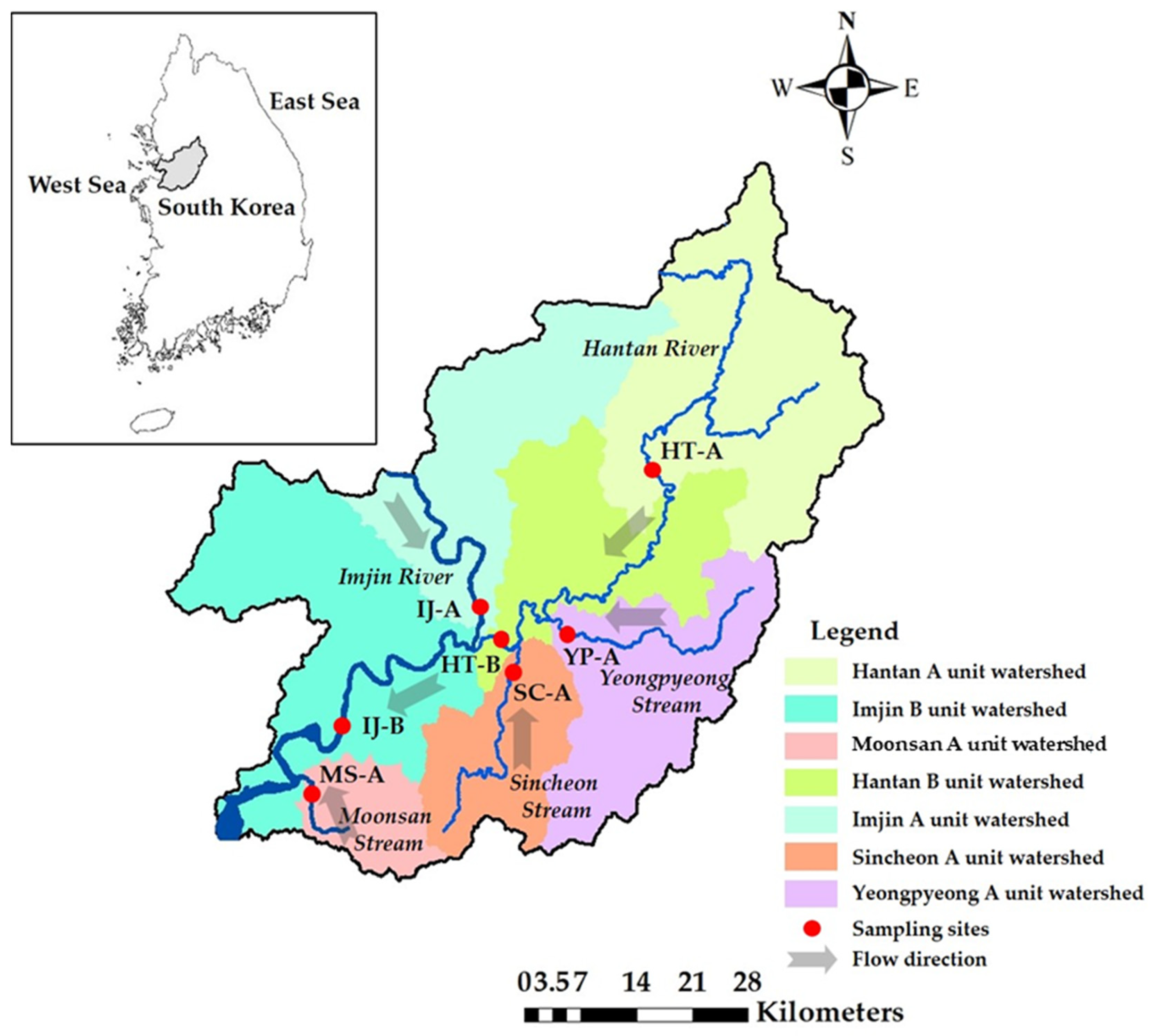
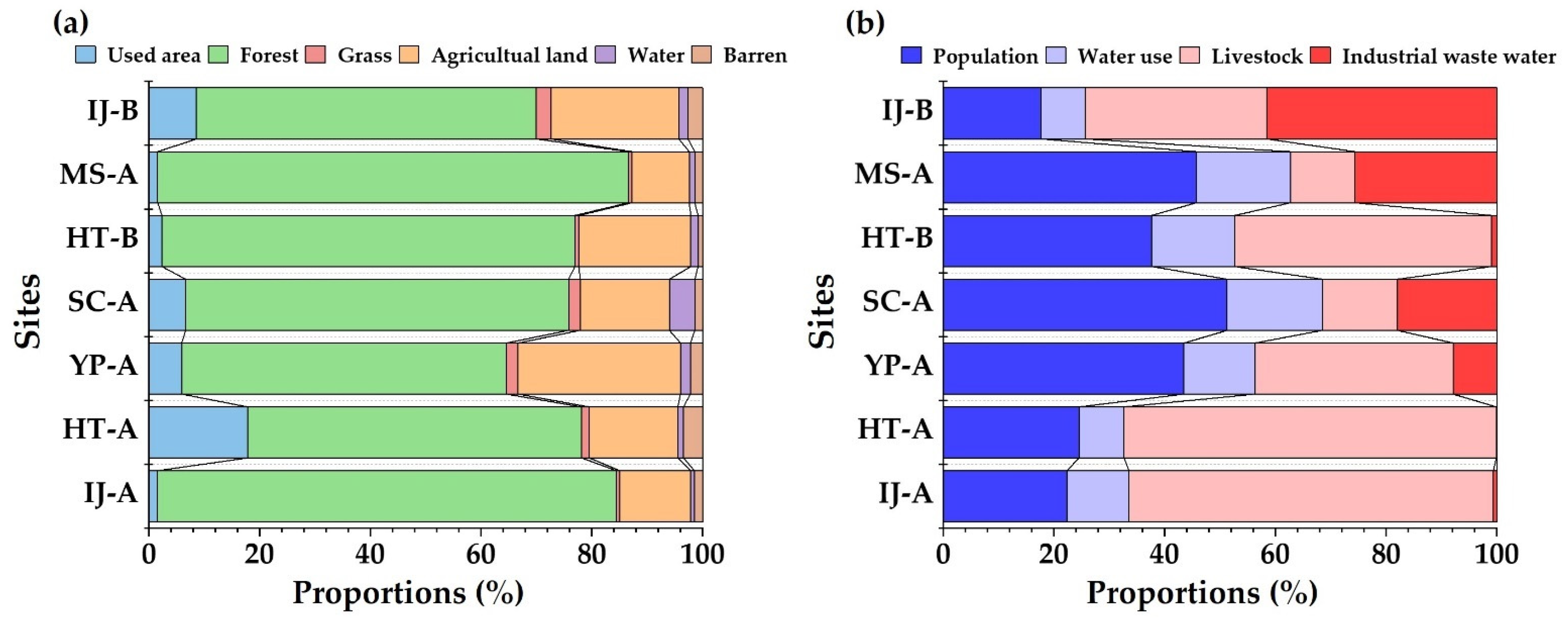
2.1. Study Area

South and North Korea on the Korean Peninsula have been divided since the Korean War (25 June 1950–27 July 1953); due to the special situation of the MDL, two countries have jointly occupied the Imjin River [39]. The Imjin River is the seventh largest river on the peninsula, originating from Duryu Mountain, Beopdong-gun, Gangwon Province, North Korea, passing through MDL, joining the Hantan River and Moonsan Stream, joining the Han River in Gimpo-si, Gyeonggi Province, and then flowing into the West Sea [38]. The Imjin River is located between 37°44′23″ N 126°31′19″ E and 37°11′12″ N 126°36′21″ E; the entire watershed area is 8139 km2, with a total length of 273.5 km [40]. This study targeted the IRW, South Korea, which accounts for 37.1% of the total watershed area, based on the MDL (Figure 1). The shape factor of the IRW is 0.126, indicating a smaller watershed width compared to the extension of the river channel [41]. The mean altitude is 680.5 m, and the elevation is between 155 and 1570 m, indicating a complex topography [40]. Mean annual precipitation of the IRW is approximately 1100 mm, of which approximately 74% occurs from June to September; it has a climate similar to a monsoon climate, with wet summers and dry winters [42]. The Ministry of Environment is currently implementing TPLMS for seven IRW watersheds [43]. Figure 2 shows the land use ratio and pollutant density ratio for each unit watershed, and that the urban and agricultural areas of IRW accounted for 24.6%. Hantan-A unit watershed had the highest percentage (17.9%) in the use of area, whereas Yeongpyeong-A unit watershed had the highest percentage (29.3%) in the agricultural area [44]. The IRW cannot be used as a drinking water source or tap water because it is impacted by tides twice a day from the estuary of the Han River to the Gorangpo point (approximately 40 km) in Yeoncheon-gun, Gyeonggi Province; hence, water is supplied from Paldang Dam of the Han River [41].

2.2. Water Sampling and Analysis

We conducted water sampling at the following water quality monitoring network points of the Ministry of Environment: Imjin River (IJ-A and IJ-B) of the main streams of the IRW; Hantan River (HT-A and HT-B), Yeongpyeong Stream (YP-A), and Shincheon Stream (SC-A); Moonsan Stream (MS-A) of the main tributaries of the IRW (Figure 1). These 7 sites were representative sites for river water quality monitoring and pollution sources management in this study [43]. Water quality samples were collected at mean intervals of 8 d from January 2019 to December 2020. The samples were analyzed for 12 water quality parameters: water temperature (WT), the potential of hydrogen (pH), electrical conductivity (EC), dissolved oxygen (DO), 5 d BOD, chemical oxygen demand (COD), suspended solids (SS), total nitrogen (TN), ammonium nitrogen (NH3-N), nitrate-nitrogen (NO3-N), TP, and phosphates phosphorous (PO4-P). WT, pH, EC, and DO were measured on site using a multiparameter sonde (EXO1, YSI Crop., Yellow Springs, OH, USA). The sample was placed in a polyethylene bottle (2 L, 3 EA) washed with 0.1 N HNO3 solution, stored in an icebox at <4 °C, and was then transported to the laboratory. BOD, COD, SS, TN, NH3-N, NO3-N, TP, and PO4-P were analyzed in the laboratory in compliance with safety regulations. Water quality sampling, preservation, transportation, and analysis were performed in line with the Water Pollution Standard Method of the Ministry of Environment [45]. The analysis methods and tools for the 12 water quality parameters are summarized in Table 1. These water variables are important indicators of water pollution showing organic, nutrient, physical, and biological properties of the river [26]. Quality assurance and quality control (QA/QC) procedures of tools and data to be analyzed were evaluated for all test items, with reference to 5% repeats, 5% spikes, standard calibration curves, and quality control reference standards [45].

2.3. Data Treatments and Multivariate Statistical Techniques

Kolmogorov–Smirnov statistics were used to test the normality of water quality data [46]. Most variables of MST should show a normal distribution; however, most variables in the raw data were far from a normal distribution with 95% confidence through statistical tests of skewness and kurtosis [26]. The water resources data collected did not meet the assumption of normality due to the survey time and location [47]. Therefore, the data were standardized (mean value: 0, standard deviation value: 1; Z-Score) to improve the explanatory power of the statistical analysis results and reduce the related errors. Standardization reduces errors due to large fluctuations in water quality data (i.e., lower effects of a unit of measure and parameter variance), and satisfies the assumption of normality for statistical analysis [3].
MST has recently been widely used as a powerful tool for research involving environmental data [24]. MST enables analysis of the relationship between different variables, and the reduction to a small number of factors from large and complex physiochemical data without the loss of information, eventually providing more accurate information regarding water quality and potential pollution sources influencing research systems [48]. In this study, we utilized MST such as hierarchical cluster analysis (HCA) and principal component analysis/factor analysis (PCA/FA), and the APCS-MLR model to identify spatiotemporal variability of IRW surface water and potential pollution sources, and to quantitatively analyze the contributions of pollution sources. An analysis was conducted by using a Z-score standardized to MST. To perform MST and the APCS-MLR model, we used the Statistical Package in the Social Science software (SPSS, v22.0; IBM Corp., Armonk, NY, USA). Data processing and basic statistical analyses (e.g., minimum, maximum, mean, standard deviation, and standard uncertainty) were performed using Excel 2019 (Microsoft Corp., Redmond, WA, USA). OriginPro 2021b (OriginLab Corp., Northampton, MA, USA) was utilized to visualize the analysis data.

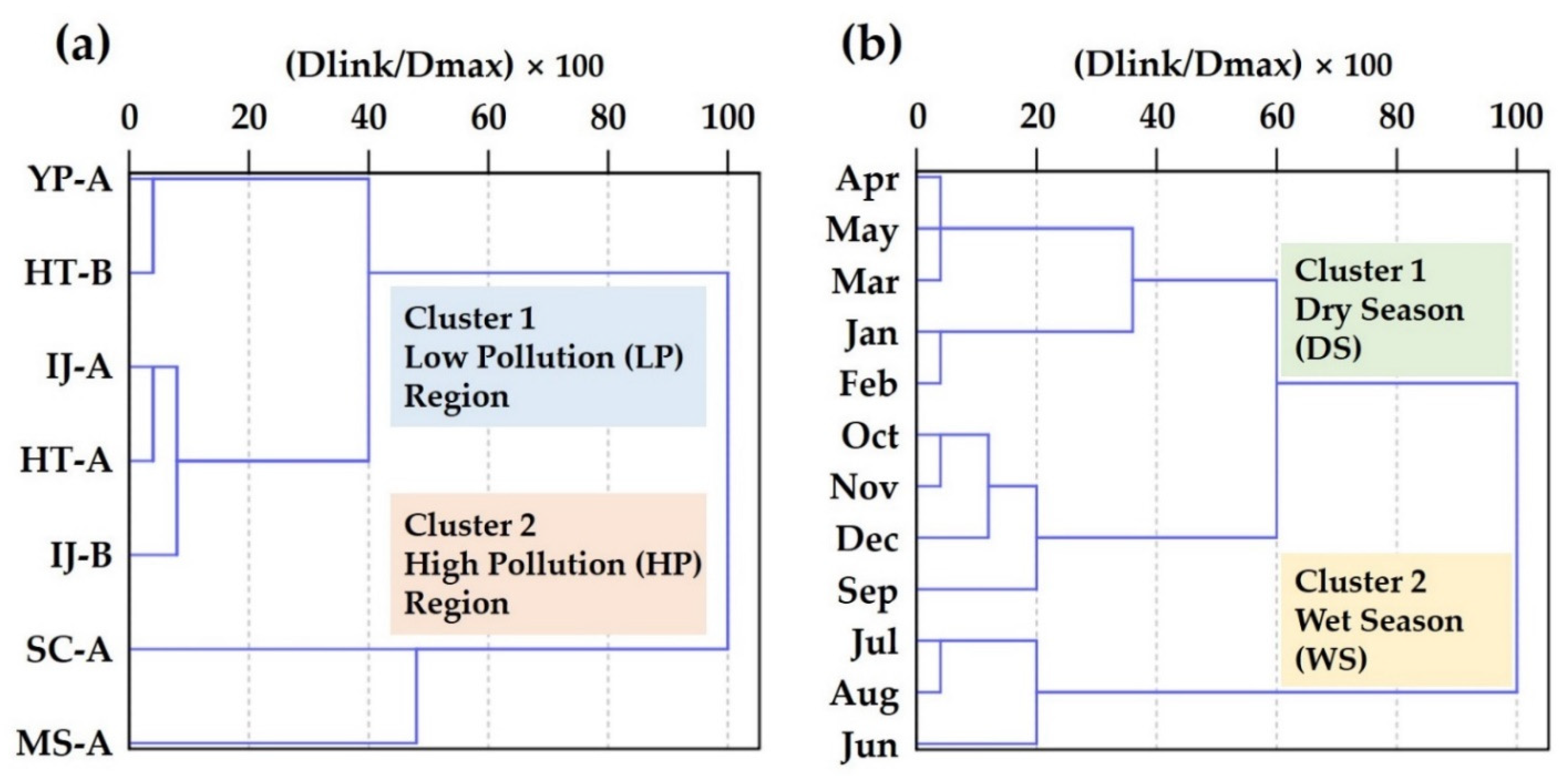
2.3.1. Cluster Analysis

Cluster analysis (CA) is an unsupervised pattern detection method that identifies the characteristics of each group after clustering large-scale data of each entity into several groups [26]. In this study, we used HCA in which clustering is sequentially performed based on distances between objects. Ward’s method and squared Euclidean distance were used for a standardized dataset to provide spatiotemporal similarity information regarding the IRW surface water [29]. Ward’s method suggests that pairs with the smallest variance are merged in a connected manner based on the variance of the entity constituting each cluster [49]. Euclidean distance indicates similarity between two samples in general; “distance” refers to the “difference” between the analyzed values of two samples [33]. HCA generated spatiotemporal dendrograms by grouping seasonal (temporal) similarities between sampling sites (spatial variability) and variables (samples). Spatiotemporal clusters were clearly identified by dendrograms with connection distances expressed as Dlink/Dmax × 100. Dlink/Dmax is a method of standardizing the connection distance expressed on the y-axis; it is reported as the value obtained by dividing the connection distance in a specific case by the maximum connection distance, multiplied by 100 [50]. Dendrograms are utilized to provide a visual summary of the clustering processes, explaining groups and proximities, and greatly reducing the dimensionality of the raw dataset [51]. As for the HCA, a one-way analysis of variance (ANOVA) was performed (p < 0.05) to analyze significant differences in spatiotemporal water quality parameters, and post hoc analysis was conducted to identify significant differences in clusters.

2.3.2. Pearson’s Correlation Analysis

Correlation analysis is a statistical technique used for testing the significance of a linear relationship between two or more variables [52]. This study obtained correlation information between water quality parameters using the Pearson’s correlation coefficient, based on a standardized Z-scale. Correlation coefficients closer to +1 or −1 indicate respectively strong positive or negative linear relationships between two variables [53]. When the correlation coefficient between two variables is zero, there is no linear relationship at the p < 0.05 level; however, a low correlation in large datasets can be strongly statistically significant at the p < 0.01 level [54].

2.3.3. Principal Component Analysis/Factor Analysis

We conducted principal component analysis (PCA) and factor analysis (FA), analyzed main factors in polluted areas grouped via HCA, and identified potential water pollution sources. PCA and FA were used as the tools for exploratory data analysis and model prediction to identify hypothetical and unobservable potential pollution sources that can trigger pollution of surface water, and to quantify pollutant source apportionment [55]. PCA is a powerful statistical method to dimensionally reduce complex multivariate datasets with linear structures and interpret them as principal components (PCs) without information loss [25]. In this study, we selected factors by considering only the PC axis for which the eigenvalue (i.e., the size of variance explaining the factor based on the Scree plot and Kaiser’s rule) was >1.0. PCA enables a rational identification of main pollution factors; however, in terms of actual controlling sources and processes, the interpretation of such factors is highly subjective and has a limitation of generalization [31]. Prior to PCA, we confirmed the basic statistics of the data via descriptive statistical analysis. In addition, the strong correlation between data was identified through Pearson’s correlation analysis; the applicability of PCA was determined through Keiser–Meyer–Olkin (KMO) and Bartlett’s test of sphericity [56]. The KMO test indicates the degree of variance caused by the PC; in general, the KMO test coefficient is between 0.5 and 0.7, which is satisfactory [57]. Bartlett’s test determines the possibility of whether a correlation matrix is a unit matrix; if the significance probability of Bartlett’s test is <0.05, it is applicable to PCA [58]. After extracting factors via PCA, FA was performed to create a new group of variables referred to as variance factors (VFs) through varimax rotation of the PCs, to clarify the factor structure in line with the correlation coefficient between factors and variables [33]. VFs were classified as “strong”, “moderate”, or “weak” if absolute loadings were >0.75, between 0.75 and 0.50, or between 0.50 and 0.30, respectively [59].

2.3.4. APCS-MLR Model

The application of the modeling, based on APCS-MLR, is known as the combination of PCA and MLR; it is generally applied to statistical techniques for source apportionment of environmental pollutants [32]. Wang et al. [60] indicated that the datasets analyzed with PCA and MLR enabled an understanding of precision and quantification of source apportion. In this study, we used PCA to determine the number and properties of potential pollution sources, and then developed the APCS-MLR model to determine the contribution of potential pollution sources. To achieve this, we first established an MLR between APCS (independent variables) and the pollutant concentration (dependent variables). We then calculated regression coefficients and quantified the contribution ratio of each PCs to the water quality variable. The source contributions to the pollutant concentration (Cj) are listed in Table S1 [30,32].
However, in the APCS-MLR model, a negative contribution ratio may appear in the calculations, misleading the accuracy of the source apportionment [60]. Negative values can be considered to be inversely related to the factor. To overcome this problem, we converted negative values to positive contributions, to indicate the contribution ratios to the water quality parameters of the corresponding water source [30,61].

3. Results and Discussion

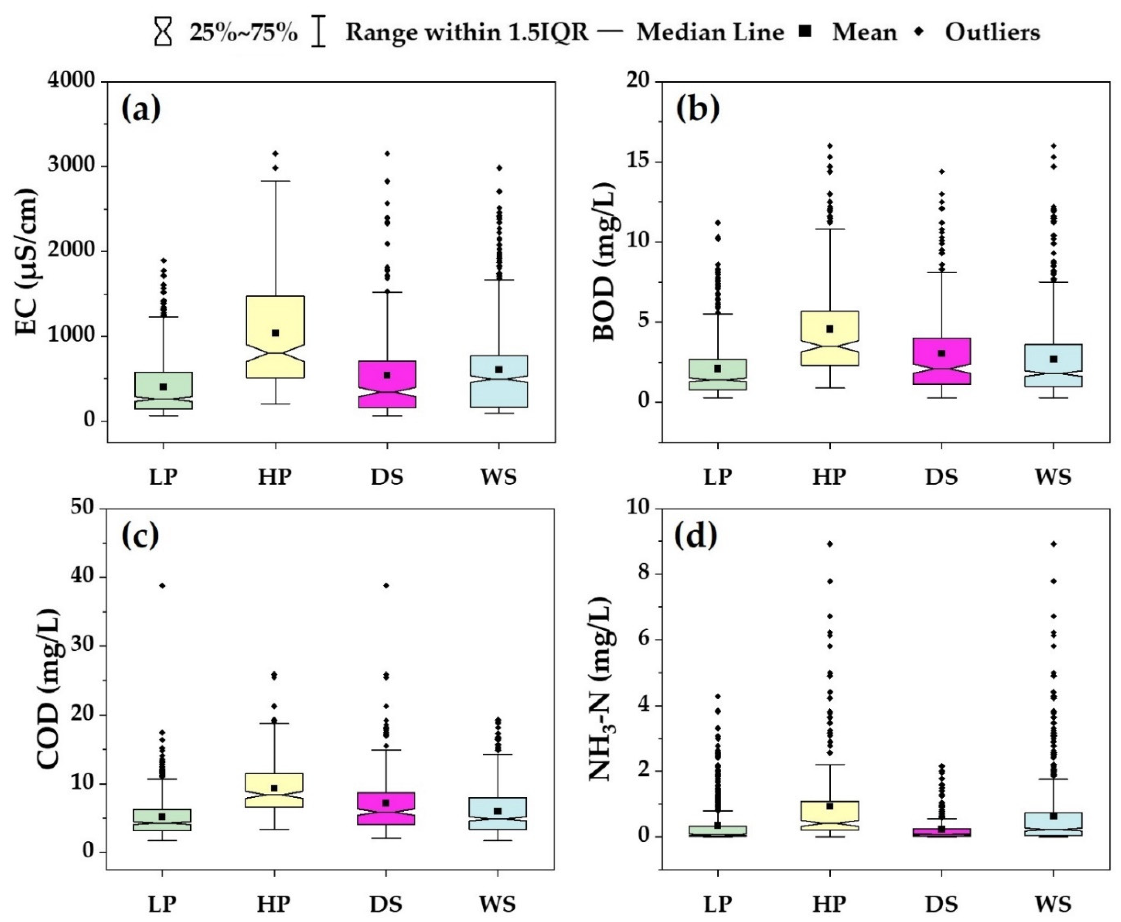
3.1. Spatial and Temporal Variations in Water Quality

Table 2 shows the descriptive statistics of 12 water quality parameters collected between 2018 and 2020 from seven water quality monitoring sites in the IRW. In terms of the spatial conditions, the IRW showed relatively high levels of BOD, COD, TN, and TP compared to the water quality standards set by the Ministry of Environment in South Korea. The spatial variation in the IRW because of anthropogenic activities and various land use types was evident [44]. The standard deviation was very large for the main streams (IJ-A and IJ-B sites), because they were more affected by summer floods than tributaries were. For the BOD, COD, TN, and TP parameters, as opposed to WT and SS, the fluctuation range was smaller for the tributary (SC-A, YP-A, and MS-A sites) than for the main stream, which may be attributed to the buffering effect of the main stream mixed with water. According to the water quality environment standards, a BOD between 1 and 10 mg/L was considered a fair grade. At sites IJ-A (0.3 mg/L) and HT-A (0.3 mg/L), the BOD was at a very good level (Ia; ≤1 mg/L). At site SC-A, on-site WT (19.5 °C) and EC (1479 µS/cm) were high compared to those elsewhere. Furthermore, the concentrations of COD (11.9 mg/L), TN (8.098 mg/L), NH3-N (1.316 mg/L), and TP (0.186 mg/L) were highest because SC-A site was significantly affected by the wastewater from textile and leather factories around the watershed [62]. At site MS-A, the mean SS concentration (55.7 mg/L) exceeded the slightly poor (IV; ≤100 mg/L) water quality standards. The high SS concentration was impacted by the low tide due to the tidal effect of the Imjin River and domestic sewage [38].
Table S2 presents the mean and standard deviation of monthly water quality parameters in the Imjin River Watershed in South Korea. Monthly BOD concentrations were maintained at slightly average (II; ≤3 mg/L) levels during September–December; however, these levels were close to the slightly bad (IV; ≤8 mg/L) levels measured in April and May. The BOD and COD concentrations were highest in spring, assumingly because of the relatively large effect of point pollution sources brought in by the low flow rate of rivers and the impact of river runoff on irrigation water carrying organic matter such as compost or fertilizer accumulated in paddy fields [63]. As shown in Table S2, TN and TP concentrations were the most polluted variables each month. The mean TN concentration was between 3.22 and 7.01 mg/L, exceeding the very poor (VI; >1.5 mg/L) level of water quality standard. The highest mean TN concentration had a large mean and standard deviation between January (6.67 mg/L) and February (7.01 mg/L). The TP concentration gradually increased from March (0.15 mg/L), reached a peak by May when there were active agricultural activities, and showed a decreasing trend between September and December, the months with the high precipitation. This reflects the complex diluting effect of the increase in river flows and other factors [63]. The TP concentrations were highest during summer due to surface runoff, and very close to the slightly poor (IV; ≤0.3 mg/L) levels of the water quality standard. Hence, water quality management is required.

3.2. Spatial and Temporal Hierarchical Agglomerative Clustering

The seven sampling sites were classified into two statistically significant clusters at (Dlink/Dmax) × 100 < 40 via spatial HCA (Figure 3a). There was a significant difference in water pollution at the sampling sites between both clusters. The cluster classifications showed spatial distribution because the sites had water quality features and natural backgrounds that were affected by similar pollution sources [47,49]. One-way ANOVA and post hoc analysis were conducted to increase the reliability and validity of HCA. The p-values of EC, BOD, COD, and NH3-N were 0.010, 0.013, 0.011, and 0.050, respectively, indicating statistically significant mean differences between clusters for each water quality parameter. By utilizing box plots [49] featuring two or more static variables, we analyzed spatial changes in EC, BOD, COD, and NH3-N water quality parameters between clusters (Figure 4). As shown in Figure 4, EC, BOD, COD, and NH3-N presented higher mean values with greater variations in cluster 2 than in cluster 1. Therefore, cluster 1 corresponded to a lower pollution (LP) region than did cluster 2. Cluster 1 encompassed sites YP-A, HT-B, and HT-A, which are located in Imjin River (IJ-A and IJ-B sites), the main stream, and Yeongpyeong Stream and Hatan River, the tributary. Sites IJ-A and HT-A are located in the upper reaches of the Imjin River and Hantan River, respectively, where there are dense forests and the only basalt in Korea. IJ-B, HT-B, and YP-A sites reflected dilution effects, mainly due to agricultural activities and anthropogenic factors [44]. In cluster 2, sites SC-A and MS-A corresponded to the high-pollution (HP) region; these two sites are located in the Shincheon Stream and Moonsan Stream, respectively. As shown in Figure 4, EC, BOD, COD, and NH3-N showed greater variability and higher mean values in the HP region than in the LP region. According to Cho et al. [38], Shincheon Stream is highly polluted by textile and leather industrial complexes, and Moonsan Stream is an area with a high rate of industrial wastewater discharge.
The temporal variability of IRW water quality was further analyzed through HCA. As for temporal HCA, we created a dendrogram by classifying 12-month mean data over 3 years (from 2018–2020) into two clusters, at (Dlink/Dmax) × 100 < 60 (Figure 3b). The two clusters corresponded to the dry and wet seasons (DS and WS, respectively) of the IRW; the DS and WS variations were statistically significant because IRW pollution was mainly affected by human activities and rainfall. Cluster 1 encompassed September–May; the cluster corresponded to DS accounting for approximately 41% of the annual mean precipitation. Cluster 2 included June–August, which corresponded to the WS and accounted for approximately 59% of the annual mean precipitation [43]. According to the measured parameter values in Table 1, the IRW had TN and TP, the most serious and concerning pollutants. In addition, EC and COD are generally considered important indicators for monitoring organic pollution in rivers, industrial water, and factory wastewater [32]. Therefore, the temporal variability of the parameters selected for DS and WS (EC, BOD, COD, and NH3-N) is shown in Figure 4b. The mean COD and NH3-N concentrations were higher in the WS than in the DS, because of the combined effect of increased surface runoff in spring and major stream inflows carrying organic matters and nitrogen from land to the aquatic environment [32,64].
As for the spatiotemporal HCA of the IRW in this study, the regional difference between LP and HP was more evident than the difference between DS and WS. Therefore, we focused on exploration and apportionment of pollution sources by performing correlation analysis of spatial groups in the IRW (LP and HP regions) and utilizing the PCA/FA or APCS-MLR model. HCA was useful in providing reliable information on spatiotemporal variability of surface water [26]. Furthermore, it was found that each cluster classified based on the characteristics of the surrounding pollution sources and monthly water quality could represent the water quality of the corresponding watershed [65]. Therefore, HCA enables the design of future optimal spatiotemporal sampling strategies by reducing the frequencies in the monitoring network and sampling, thereby reducing costs without losing the significance of the results [66].

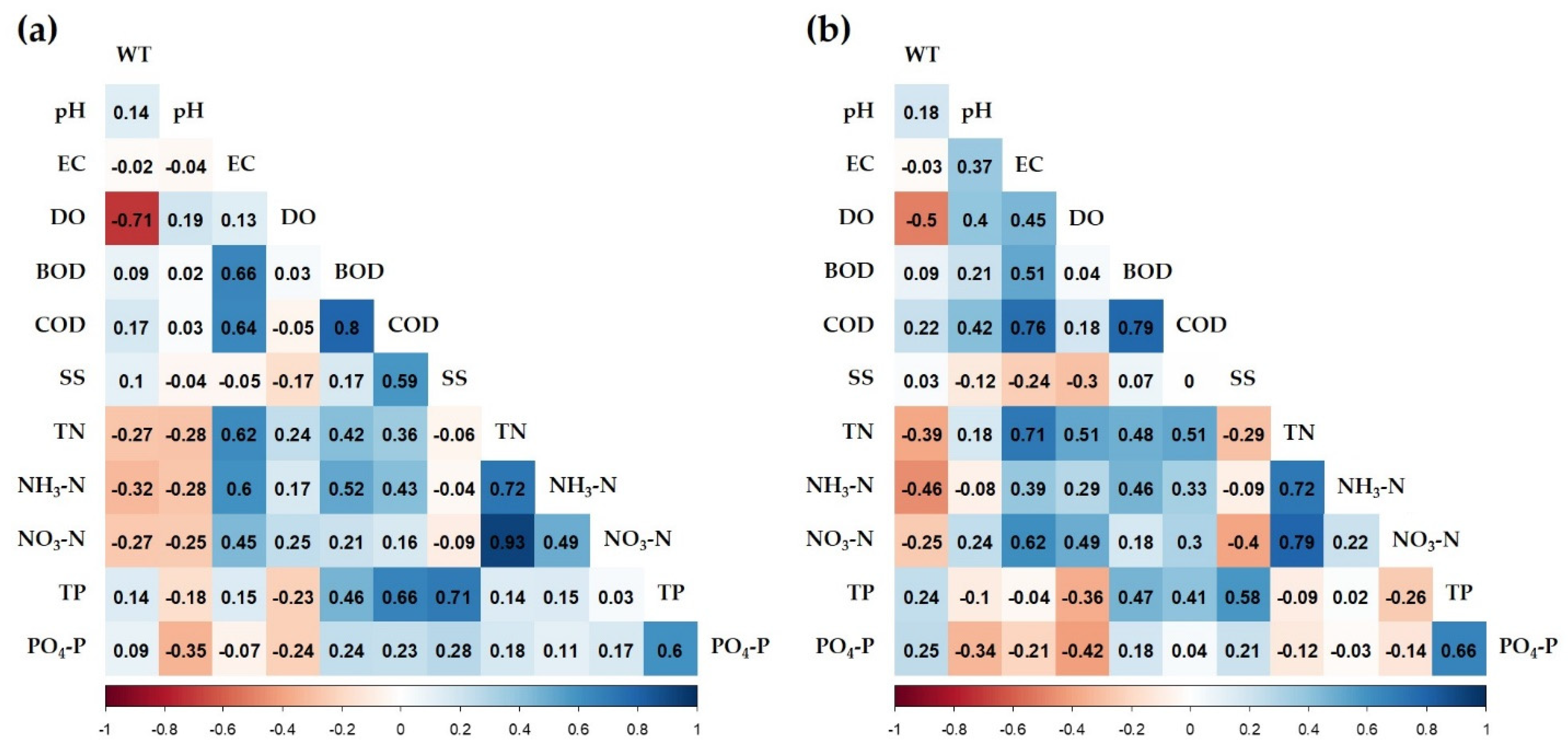
3.3. Correlation Analysis of Water Quality Parameters According to Polluted Region

To provide correlation information between physicochemical water quality parameters of spatially clustered LP and HP regions through HCA, the Pearson’s correlation coefficient (r) with statistical significance was used (p < 0.05). As indicated in Figure 5, the correlation analysis for the IRW showed the following: EC had a positive (+) correlation with the concentrations of organic matter and nitrogen-based substances, and SS and PO4-P had a negative (−) correlation. Such correlations were more obvious in the HP region than in the LP region. Furthermore, SS and PO4-P showed negative (−) correlations with pH, EC, and DO. The negative (−) correlation between WT and DO was statistically stronger in the LP region than in the HP region (r = −0.71, p < 0.01). The statistically strong positive (+) correlations between EC, and COD, TN, and NO3-N were predominant in the HP region (r > 0.60, p < 0.01). The reason is that the Shincheon and Moonsan Streams in the HP region showed high densities of nondegradable materials and industrial wastewater discharge due to textile factories and large-scale industrial facilities around the streams [67]. In the LP region, EC had a statistically strong positive (+) correlation with BOD and NH3-N (r > 0.60, p < 0.01). There was a strong positive (+) correlation between SS and COD concentrations (r = 0.59, p < 0.01) in the LP region; however, there was no statistically significant correlation in the HP region. The statistically strong positive (+) correlations between BOD, and TN and TP were more prominent in the HP region than in the LP region (r > 0.47, p < 0.01). On the basis of these correlations, organic matters in the HP region were confirmed to flow into the river along with nutrients [68].

3.4. Pollution Source Identification Using PCA/FA

PCA/FA was performed on the standardized data to identify the factors affecting water quality in the LP and HP regions clustered by HCA. The KMO test values for LP and HP regions were 0.592 and 0.621, respectively, and Bartlett’s sphericity test value was 0.00 (p < 0.01), indicating that there was a statistical significance for the correlation between water quality parameters, and the conformance of PCA [28]. PCA/FA extracted four and three PCs with an eigenvalue of >1 for the LP and HP regions, respectively. This explained approximately 80.8% and 72.0% of the total variance for the water quality datasets for the LP and HP regions, respectively. Table 3 summarizes the PCA/FA results, including loading, eigenvalues, variance, and cumulative variance for each VF.
VF1 in the LP region accounted for 29.37% of the total variance with strong positive loadings (0.90, 0.83, and 0.78, respectively) for EC, TN, and NH3-N, and with medium positive loadings (0.74 and 0.65, respectively) for BOD and NO3-N. EC and TN of surface water can originate from pollution sources including fertilizer use, animal waste, and domestic and industrial sewage [69]. Five sites in the LP region are dominated by mountains, grasslands, and agricultural lands. Since the LP region has low population density and there has been minimal exploitation, it appeared to be mostly related to agriculture and livestock, and to be more impacted by manure and chemical fertilizers than by industrial sewage [32]. Nitrogen from agricultural land and pasture in the LP region flows into rivers in the vicinity due to surface runoff and flooding irrigation, as primary fertilizer for crops and general livestock waste. Studies on the Nakdong River in South Korea, Grand River in the USA, and Min River in China also revealed that EC and TN were the most influential parameters in VF1 in terms of agricultural areas through PCA/FA [70,71,72]. Therefore, VF1 in the LP region can be considered a nonpoint source due to agricultural activities. VF2 in the LP region accounted for 21.49% of the total variance with strong positive loadings (0.90 and 0.87, respectively) for TP and SS, and with medium positive loading (0.71) for COD. This factor can be regarded as the accumulated organic pollutants from the discharge of untreated wastewater, including domestic and industrial wastewater [61]. VF3 had a strong negative loading (−0.92) for water temperature, whereas it accounted for 15.70% of the total variance with strong positive loading (0.88) for DO. WT and DO are commonly considered as factors of seasonal variation [65]. VF4 accounted for 14.19% of the total variance with a strong negative loading (−0.82) for pH, and with a medium positive loading (0.62) for PO4-P. This can be regarded as the physicochemical variability of the river [72].
VF1 accounted for 29.40% of the total variance in the HP region and provided strong positive loading (i.e., 0.95, 0.83, and 0.80, respectively) for COD, EC, and BOD and a medium positive loading (0.54) for pH. VF1 of HP region was associated with various organic matter sources of industrial wastewater, and municipal sewage [66]. According to Choi et al. [67], Shincheon Stream and Moonsan Stream in the HP region showed the high industrial wastewater discharge density and the discharge of a large amount of industrial wastewater into rivers and ditches in the vicinity without proper treatment, which indicates that the streams have been greatly influenced by urbanization and industrialization. The SC-A site, where there were impacts of effluent from textile factories and basic treatment facilities, indicated the highest mean concentrations of variables such as EC, BOD, COD, TN, TP, NH3-N, and NO3-N. The mean NH3-N concentration, a toxicity indicator of river odor and degraded health of aquatic organisms [67], was 1.32 mg/L at site SC-A, which was less than the US EPA standard of 1.9 mg/L; however, it requires strict management. Therefore, VF1 in the HP region can be interpreted as being affected by point pollution sources from municipal and industrial sewage discharges. VF2 accounted for 24.13% of the total variance, and showed strong positive loadings (0.86 and 0.75, respectively) for TP and PO4-P, a medium loading (0.63) for SS, and negative loadings (−0.64 and −0.49, respectively) for DO and NO3-N. Since SS is partially related to surface runoff and phosphorus flow into rivers with surface runoff [65], VF2 in the HP region can be attributed to municipal sewage triggered by surface runoff. VF3 accounted for 24.3% of the total variance and indicated a strong negative loading (−0.82) for WT, a positive loading (0.78) for NH3-N, and a medium positive loading (0.65) for TN. WT is related to seasonal effects, and nitrogen fertilizers may be a major source from agricultural activities [73]. As a result, it can be considered that VF2 in the HP region was affected by nonpoint source pollution, as nitrogen fertilizers have been shown to contribute to river loadings via agricultural activities [32].
After identifying potential pollution sources using PCA/FA, MLR analysis was performed on VFs in LP and HP regions. The R2 values in Table 4 range between 0.883 and 0.971, which is closer to 1; the prediction of the corresponding regression equation can be considered valid. Of the information of the dependent variable VFs, 88.3–97.1% can be considered as the variation in the independent variable. Furthermore, as the standard error of the estimate was <0.5, it can be determined as a valid regression equation. As a result of one-way ANOVA, as the probability value (p-value) of the F statistics was less than the significance level of 0.001, the corresponding regression equation can be considered statistically significant.

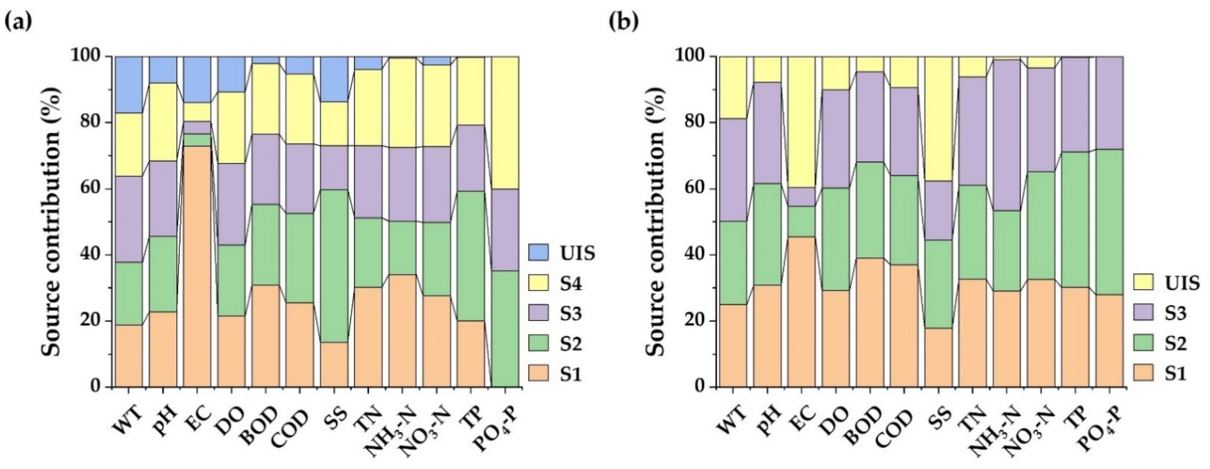
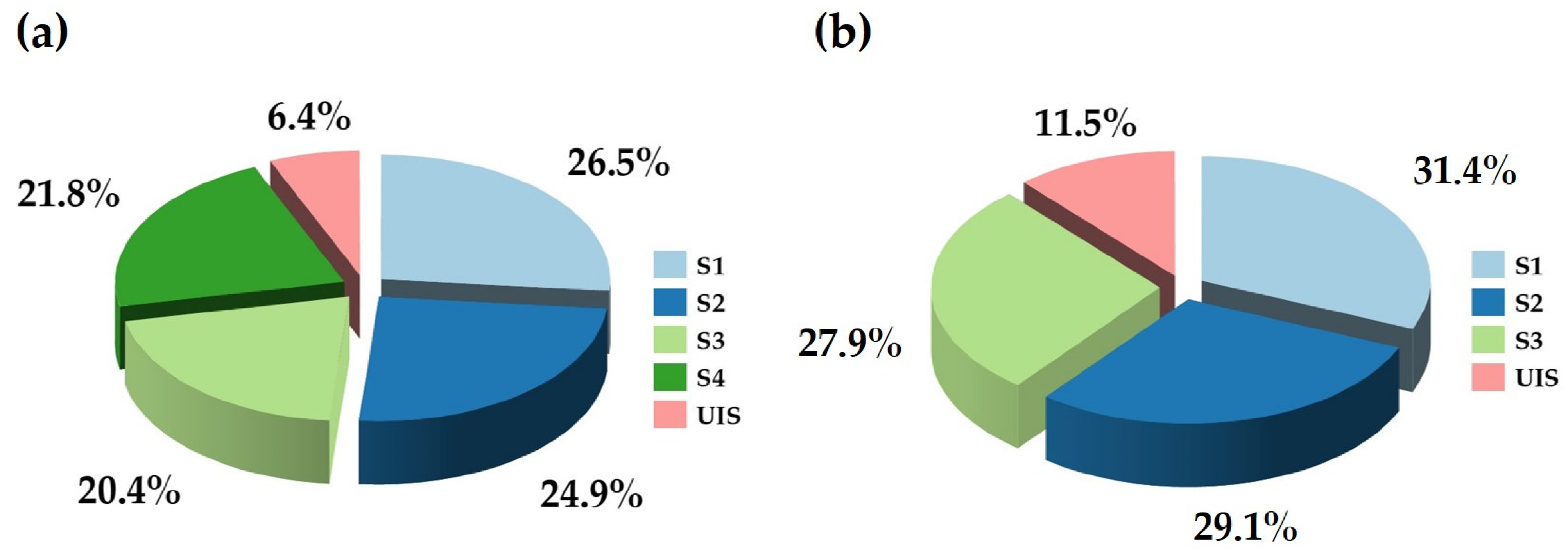
3.5. Pollution Source Apportionment Using APCS-MLR Model

We analyzed the APCS-MLR model to quantify the contribution of each pollution source to 12 water quality parameters in the LP and HP regions (Figure 6). MLR analysis for the LP and HP regions showed a good model with consistency between the measured and predicted values >0.6, except for the relatively lower determination coefficient (R2 = 0.396) for SS in the HP region. According to Gholizadeh et al. [30], in general, when the coefficient of determination (R2) is >0.5, there is a good consistency between observed and predicted values, and a reliable assessment of pollution source apportionment can be made. Figure 7 indicates the mean contributions of pollution sources using the APCS-MLR model in the LP and HP regions.
Source 1 (S1, 26.5%) in the LP region was greatly affected by nonpoint source pollution, mainly from agricultural activities. Nonpoint source pollution accounted for 26.5% of the total pollution sources and showed high contribution ratios in the nitrogen series (NH3-N, 34.1%; TN, 30.3%; NO3-N, 27.6%), EC (73.0%), and BOD (30.8%) water quality parameters. Furthermore, organic pollution (S2) from domestic sewage and industrial wastewater accounted for 24.9% of the entire pollution sources and showed high contribution ratios in SS (46.2%), TP (39.3%), PO4-P (35.2%), and COD (27.0%) water quality parameters. Physicochemical effects (S3) accounted for 21.8% of the total pollution sources, and mainly showed the contribution ratio of 23.5%, mainly in pH. Seasonal effects on diverse water quality parameters (S4, 20.4%) showed contribution ratios in WT and DO of 26.2% and 24.6%, respectively. Through the APCS-MLR model, unidentified source (UIS) estimated water quality parameters contributing to river water pollution ranging from 0.1% (TP) to 17.1% (WT). According to Zhang et al. [74], since the estimated contributions of UIS consist of a mixture of pollutants, and originate from complex sources, the identification of sources via the APCS-MLR model could be problematic. Therefore, the contributions of pollution sources in the LP area were determined as being in the following descending order: Nonpoint source pollution from agricultural activities (S1, 26.5%), point pollution sources from domestic sewage and industrial wastewater (S2, 24.9%), physicochemical effects (S4, 21.8%), seasonal effects (S3, 20.4%), and UIS (6.4%).
Most water quality parameters in the HP region were significantly affected by point pollution sources from domestic sewage and industrial wastewater (S1, 31.4%). This was shown by the high contribution ratios of organic pollution sources (BOD, 39.1%; COD, 37.1%) and physicochemical effects (EC, 45.4%; pH, 30.9%) to river water quality. Point source pollution from municipal sewage (S2) accounted for 29.1% of the total pollution sources, and phosphorus-based substances were present (TP, 40.9%; PO4-P, 43.9%). The impact of nonpoint source pollution from agricultural activities (S3) accounted for 27.9% of the total pollution sources in TN (32.8%) and NH3-N (45.7%); seasonal effects had the greatest impact on WT (31.1%). As shown in Figure 4, UIS in the HP region estimated water quality parameters contributing to river water pollution ranging between 0.04% (PO4-P) and 39.6% (EC). Therefore, the pollution sources in the HP region descended in the following order: Point source from domestic sewage and industrial wastewater (S1, 31.4%), point source from urban sewage (S2, 29.1%), nonpoint source pollution from agricultural activities or seasonal effects (S3, 27.9%), and UIS (11.5%) (Figure 7). Therefore, it was demonstrated that the APCS-MLR model was able to quantify the source contribution to physicochemical water quality parameters in the LP and HP regions.

3.6. Strengths and Limitations

Several advantages and limitations were identified in this study. First, MST and the APCS-MLR model used in this study were useful tools for identifying hidden relationships and factors regarding large and complex water quality datasets, and for providing environmental information influencing environmental systems. Second, in the field of water environment research, MST and the APCS-MLR model have shown reliability and validity in water quality assessments of the target watershed, and the results are useful for water environment protection and water resource management policies in the future. Third, customized water quality assessment and management of the target watershed required the identification of potential pollution sources, by determining the main factors based on spatial conditions and quantitatively analyzing the contributions of pollution sources. However, we must consider the following limitations in interpreting the study results. First, the Imjin River on the Korean Peninsula is a transboundary river between South and North Korea, and it was hard to access to obtain necessary information for water quality data analysis of the IRW in North Korea due to the MDL and political conditions, given that the entire watershed of the river could not be evaluated. Second, we were not able to evaluate the variability of physicochemical water quality parameters (discharge, fecal coliform, and chlorophyll-a) that were not selected in this study. Third, we could not investigate unidentified pollution sources in the target watershed. Therefore, in the future, a highly reliable water quality assessment of the target watershed should consider the limitations of this study and will require additional research. Finally, there are many acronyms in this study. Therefore, all acronyms and their meanings were summarized in Table S3.

4. Conclusions

In this study, we combined MSA (such as HCA and PCA/FA) and the APCS-MLR model to identify spatiotemporal variability of water quality in the IRW, distinguish potential pollution sources, and apportion the pollution sources. To assess the water quality of the IRW, we selected seven monitoring sites (IJ-A, HT-A, YP-A, SC-A, HT-B, MS-A, and IJ-B) and analyzed 12 water quality parameters (WT, pH, EC, DO, BOD, COD, SS, TN, NH3-N, NO3-N, TP, and PO4-P). At the seven water quality monitoring sites, while reflecting the impacts of anthropogenic activities and different land use types, significant changes in physicochemical water quality parameters were observed. In particular, at the SC-A site, parameters such as WT, EC, BOD, COD, TN, NH3-N, and TP indicated high concentrations; this can be interpreted as meaning that the site was considerably impacted by textile and leather factories around the watershed. Spatial HCA classified the seven monitoring sites into two clusters, corresponding to LP and HP regions, in which there was a statistically significant correlation (p < 0.01) between nitrogenous (TN and NO3-N, r = 0.93) and organic matter (BOD and COD, r = 0.79) variables, respectively. The PCA/FA results showed that LP and HP regions were significantly affected by different pollution factors. The LP region was mainly affected by nonpoint source pollution, mainly from agricultural activities; whereas, in the HP region, a large amount of industrial wastewater and domestic sewage flowed into the river, and organic matters and nutrient salts accumulated in the surface water. The APCS-MLR model revealed that nonpoint source pollution from agricultural activities (26.5%) was the crucial pollution source in the LP region, whereas point sources from domestic sewage and industrial wastewater (31.4%) were the main contributors in the HP region.
This study showed that MST and the APCS-MLR model are useful tools for understanding spatiotemporal water quality changes and identifying and apportioning potential pollution sources, for efficient water quality management in the IRW. Currently, TPLMS has been implemented in seven watersheds in the IRW to maintain target water quality (BOD and TP); however, if appropriate water quality management policies are not enacted for the watershed, water quality will inevitably deteriorate in the future. Therefore, the priorities in the LP region should be as follows: (1) reduction of fertilizer in rural areas, control of pesticide uses, and optimization for livestock breeding management; (2) reduction of nonpoint source pollution, i.e., pilot projects should be implemented for rainwater runoff treatment facilities and rainwater pumping station reservoirs. In the HP region, there should be (1) reinforcement of effluent operation standards of wastewater treatment facilities, and application of advanced wastewater reduction treatment technology; (2) TPLMS implementation reviews for tributaries, in order to control pollutant discharges to tributaries; (3) improvement of individual treatment capacities of domestic sewage. This study can assist water quality managers and policymakers to comprehensively understand the main pollution sources in terms of spatial conditions, and to determine the priorities for water quality improvement regarding water pollution control and sustainable development in Imjin River, South Korea.

Supplementary Materials

The following supporting information can be downloaded at https://www.mdpi.com/article/10.3390/w14050793/s1: Table S1: Factors and calculations considered for the APCS-MLR model, Table S2: Mean and standard deviation (SD) of water quality parameters during different months in the Imjin River Watershed, South Korea, Table S3: Summary of all acronyms in this study.

Author Contributions

Conceptualization, Y.-C.C. and J.-K.I.; methodology, H.C. and M.-G.L.; software, Y.-C.C.; validation, Y.-C.C. and H.C.; formal analysis, Y.-C.C.; investigation, H.C., M.-G.L., and S.-H.K.; resources, S.-H.K.; data curation, Y.-C.C.; writing—original draft preparation, Y.-C.C. and J.-K.I.; writing—review and editing, Y.-C.C., H.C., M.-G.L., S.-H.K. and J.-K.I.; visualization, Y.-C.C. and H.C.; supervision, S.-H.K.; project administration, S.-H.K.; funding acquisition, S.-H.K. All authors have read and agreed to the published version of the manuscript.

Funding

This research was supported by the National Institute of Environmental Research (NIER) (grant number NIER-2021-01-01-134), funded by the Ministry of Environment (MOE) of the Republic of Korea.

Institutional Review Board Statement

Not applicable.

Informed Consent Statement

Not applicable.

Data Availability Statement

Not applicable.

Conflicts of Interest

The authors declare no conflict of interest.

References

  1. Cosgrove, W.J.; Loucks, D.P. Water management: Current and future challenges and research directions. Water Resour. Res. 2015, 51, 4823–4839. [Google Scholar] [CrossRef] [Green Version]
  2. Kumar, V.; Sharma, A.; Kumar, R.; Bhardwaj, R.; Thukral, A.K.; Rodrigo-Comino, J. Assessment of heavy-metal pollution in three different Indian water bodies by combination of multivariate analysis and water pollution indices. Hum. Ecol. Risk Assess. 2020, 26, 146–161. [Google Scholar] [CrossRef]
  3. Bhat, S.U.; Bhat, A.A.; Jehangir, A.; Hamid, A.; Sabha, I.; Qayoom, U. Water quality characterization of Marusudar River in Chenab Sub-Basin of North-Western Himalaya using multivariate statistical methods. Water Air Soil Pollut. 2021, 232, 449. [Google Scholar] [CrossRef]
  4. Mir, R.A.; Gani, K.M. Water quality evaluation of the upper stretch of the river Jhelum using multivariate statistical techniques. Arap. J. Geosci. 2019, 12, 445. [Google Scholar] [CrossRef]
  5. Isiyaka, H.A.; Mustapha, A.; Juahir, H.; Phil-Eze, P. Water quality modelling using artificial neural network and multivariate statistical techniques. Model. Earth Syst. Environ. 2018, 5, 583–593. [Google Scholar] [CrossRef]
  6. Sun, X.; Zhang, H.; Zhong, M.; Wang, Z.; Liang, X.; Huang, T.; Huang, H. Analyses on the temporal and spatial characteristics of water quality in a seagoing river using multivariate statistical techniques: A case study in the Duliujian River, China. Int. J. Environ. Res. Public Health 2019, 16, 1020. [Google Scholar] [CrossRef] [PubMed] [Green Version]
  7. Chen, J.; Lu, J. Effects of land use, topography and socio-economic factors on river water quality in a mountainous watershed with intensive agricultural production in east China. PLoS ONE 2014, 9, e102714. [Google Scholar] [CrossRef] [PubMed]
  8. Huang, J.; Zhang, Y.; Bing, H.; Peng, J.; Dong, F.; Gao, J.; Arhonditsis, G.B. Characterizing the river water quality in China: Recent progress and on-going challenges. Water Res. 2021, 201, 117309. [Google Scholar] [CrossRef]
  9. Dutta, S.; Dwivedi, A.; Kumar, M.S. Use of water quality index and multivariate statistical techniques for the assessment of spatial variations in water quality of a small river. Environ. Monit. Assess. 2018, 190, 718. [Google Scholar] [CrossRef]
  10. Yotova, G.; Varbanov, M.; Tcherkezova, E.; Tsakovski, S. Water quality assessment of a river catchment by the composite water quality index and self-organizing maps. Ecol. Indic. 2021, 120, 106872. [Google Scholar] [CrossRef]
  11. Ding, J.; Jiang, Y.; Fu, L.; Peng, Q.; Kang, M. Imfacts of land use on surface water quality in Subtropical River Basin: A case study of the Dongjiang River Basin, Southeastern China. Water 2015, 7, 4427–4445. [Google Scholar] [CrossRef] [Green Version]
  12. Gupta, M.; Santoro, D.H.D.; Torfs, E.; Doucet, J.; Van, P.; Vanrolleghen, A.A.; Nakhla, G. Experimental assessment and validation of quantification method for cellulose content in muncipal waste water and sludge. Envion. Sci. Pollut. Res. Int. 2018, 25, 16743–16753. [Google Scholar] [CrossRef]
  13. Gruss, L.; Wiatkowski, M.; Pulikowski, K.; Klos, A. Determination of change in the quality of surface water in the River-Reservoir system. Sustainability 2021, 13, 3457. [Google Scholar] [CrossRef]
  14. United States Environment Protection Agency. Available online: http://epa.gov/waterdata (accessed on 11 October 2021).
  15. United States Geological Survey. Available online: http://usgs.gov/missin-areas/water-resources/data (accessed on 15 October 2021).
  16. Hong, Z.; Zhao, Q.; Chang, J.; Peng, L.; Wang, S.; Hong, Y.; Liu, G.; Ding, S. Evaluation of water quality and heavy metal in wetlands along the yellow river in Henan province. Sustainability 2020, 12, 1300. [Google Scholar] [CrossRef] [Green Version]
  17. Nasir, M.F.M.; Samsudin, M.S.; Mohamad, I.; Awaluddin, M.R.A.; Mansor, M.A.; Juahir, H.; Ramli, N. River water quality modeling using combined principle component alalysis (PCA) and multiple linear regressions (MLR): A case study at Klang River, Malaysia. World Appl. Sci. J. 2011, 14, 73–82. [Google Scholar]
  18. Sotomayor, G.; Hampel, H.; Vazquea, R. Water quality assessment with emphasis in parameter optiomisation using pattern recognition methods and genetic algorithm. Water Res. 2018, 130, 353–362. [Google Scholar] [CrossRef] [PubMed]
  19. Kazi, T.G.; Arain, M.B.; Jamali, M.K.; Jalbani, N.; Afridi, H.I.; Sarfraz, R.A.; Baig, J.A.; Shah, A.Q. Assessment of water quality of polluted lake using multivariate statistical techniques: A case study. Ecotox. Environ. Saf. 2009, 72, 301–309. [Google Scholar] [CrossRef] [PubMed]
  20. Katyal, D. Water quality indices used for surface water vulnerability assessment. Int. J. Environ. Sci. 2011, 2, 154–173. [Google Scholar]
  21. Liu, W.; Li, S.; Bu, H.; Zhang, Q.; Liu, G. Eutrophication in the Yunnan Plateau Lakes: The influence of lake morphology, watershed land use, and socioeconomic factors. Environ. Sci. Pollut. Res. Int. 2012, 19, 858–870. [Google Scholar] [CrossRef] [PubMed]
  22. Kamboj, N.; Kamboj, V. Water quality assessment using overall index of pollution in riverbed-mining area of Ganga-River Haridwar India. Water Sci. 2019, 33, 65–74. [Google Scholar] [CrossRef] [Green Version]
  23. Tomczyk, P.; Wiatkowski, M.; Gruss, L. Application of macrophytes to the assessment and classification of ecological status above and below the barrage with hydroelectric building. Water 2019, 11, 1028. [Google Scholar] [CrossRef] [Green Version]
  24. Wang, J.; Liu, G.; Liu, H.; Lam, P.K.S. Multivariate statistical evaluation of dissolved trace elements and a water quality assessment in the middle reaches of Huaihe River, Anhui, China. Sci. Environ. 2017, 583, 421–431. [Google Scholar] [CrossRef] [PubMed]
  25. Mohanty, C.R.; Nayak, S.K. Assessment of seasonal variations in water quality of Brahmani river using PCA. Adv. Environ. Res. 2017, 6, 53–65. [Google Scholar] [CrossRef]
  26. Chen, P.; Li, L.; Zhang, H. Spatio-Temporal variations and source apportionment of water pollution in Danjiangkou Reservoir Basin, Central China. Water 2015, 7, 2591–2611. [Google Scholar] [CrossRef] [Green Version]
  27. Choi, H.; Cho, Y.C.; Kim, S.H.; Yu, S.J.; Im, J.K. Water quality assessment and potential source contribution using multivariate statistical techniques in Jinwi river, South Korea. Water 2021, 13, 2976. [Google Scholar] [CrossRef]
  28. Chen, S.; Tang, Z.; Wang, J.; Wu, J.; Yang, C.; Kang, W.; Huang, X. Multivariate analysis and geochemical signatures of shallow groundwater in the main urban area of Chongqing, Southwestern China. Water 2020, 12, 2833. [Google Scholar] [CrossRef]
  29. Mahmoud, M.T.; Hamouda, M.A.; Al Kendi, R.R.; Mohamed, M.M. Health risk assessment of household drinking water in a district in the UAE. Water 2018, 10, 1726. [Google Scholar] [CrossRef] [Green Version]
  30. Gholizadeh, M.H.; Melesse, A.M.; Reddi, L. Water quality assessment and apportionment of pollution source using APCS-MLR and PMF receptor modeling techniques in three major rivers of South Florida. Sci. Total Environ. 2016, 566–567, 1552–1567. [Google Scholar] [CrossRef] [PubMed]
  31. Samsudin, M.S.; Azid, A.; Khalit, S.I.; Saudi, A.S.M.; Zaudi, M.A. River water quality assessment using APCS-MLR and statistical process control in Johor River Basin, Malaysis. Int. J. Adv. Appl. Sci. 2017, 4, 84–97. [Google Scholar] [CrossRef] [Green Version]
  32. Zhang, H.; Li, H.; Yu, H.; Siquan, C. Water quality assessment and pollution source apportionment using multi-statistic and APCS-MLR modeling techniques in Min River Basin, China. Environ. Sci. Pollut. Res. 2020, 27, 41987–42000. [Google Scholar] [CrossRef]
  33. Su, J.; Qiu, Y.; Lu, Y.; Yang, X.; Li, S. Use of multivariate techniques to study spatial variability and sources apportionment of pollution in rives flowing into the Laizhou Bay In Dongying District. Water 2021, 12, 772. [Google Scholar] [CrossRef]
  34. Ahmed, F.; Fakhruddin, A.N.M.; Imam, M.T.; Khan, N.; Abdullah, A.T.M.; Khan, T.A.; Rahman, M.M.; Uddin, M.N. Assessment of roadside surface water quality of Savar, Dhaka, Bangladesh using GIS and multivivariate statistical techniques. Appl. Water Sci. 2017, 7, 3511–3525. [Google Scholar] [CrossRef] [Green Version]
  35. Bhuiyan, M.A.H.; Rakib, M.A.; Dampare, S.B.; Ganyaglo, S.; Suzuki, S. Surface water quality assessment in the central part of Bangladesh using multivariate analysis. KSCE J. Civ. Eng. 2011, 15, 995–1003. [Google Scholar] [CrossRef]
  36. Kim, D.; Lee, H.; Jung, H.C.; Hwang, E.; Hossain, F.; Bonnema, M.; Kang, D.H.; Getirana, A. Monitoring river basin development and variation in water resources in transboundary Imjin River in North and South Korea using remote sensing. Remote Sens. 2020, 12, 195. [Google Scholar] [CrossRef] [Green Version]
  37. Ministry of Environment (MOE). Study on Application Method of Watershed Model for Total Water Pollutant Load Management (TPLMS); Ministry of Environment: Sejong, Korea, 2010.
  38. Cho, Y.C.; Choi, H.M.; Lee, Y.J.; Ryu, I.; Lee, M.G.; Gu, D.; Choi, K.; Yu, S. Statistical analysis of water flow and water quality data in the Imjin River Basin for total pollutant load management. J. Environ. Assess. 2018, 27, 353–366. [Google Scholar]
  39. Ha, D.T.T.; Kim, S.H.; Bae, D.H. Impacts of upstream structures in downstream discharge in the transboundary Imjin River, Korea Peninsula. Appl. Sci. 2020, 10, 3333. [Google Scholar] [CrossRef]
  40. Jabbari, A.; Bae, D.H. Application of artificial neural networks for accuracy enhancements of real-time flood forecasting in the Imjin Basin. Water 2018, 10, 1626. [Google Scholar] [CrossRef] [Green Version]
  41. Kim, D.P.; Kim, K.H.; Kim, J.H. Runoff estimation of Imjin River Basin through April 5th Dam and Hwangang Dam Construction of North Korea. J. Environ. Sci. 2011, 20, 1635–1646. [Google Scholar]
  42. Jabbari, A.; So, J.M.; Bae, D.H. Precipitation forecast contribution assessment in the coupled meteo-hydrological models. Atmosphere 2020, 11, 34. [Google Scholar] [CrossRef] [Green Version]
  43. Ministry of Environment (MOE). Operation for Streamflow Monitoring Network in Han River Basin; Ministry of Environment: Sejong, Korea, 2020.
  44. Park, M.; Cho, Y.; Shin, K.; Shin, H.; Kim, S.; Yu, S. Analysis of water quality characteristics in unit watershed in the Hangang Basin with respect to TMDL implementation. Sustainability 2021, 13, 9999. [Google Scholar] [CrossRef]
  45. Ministry of Environment (MOE). Official Testing Method with Respect to Water Pollution Process; Ministry of Environment: Sejong, Korea, 2018.
  46. Putri, M.S.A.; Lou, C.H.; Syai’in, M.; Ou, S.H.; Wang, Y.C. Long-Term river water quality trends and pollution source apportionment in Taiwan. Water 2018, 10, 1394. [Google Scholar] [CrossRef] [Green Version]
  47. Wang, X.; Cai, Q.; Ye, L.; Qu, X. Evaluation of spatial and temporal variation in stream water quality by multivariate statistical techniques: A case study of the Xiangxi River basin, China. Quat. Int. 2012, 282, 137–144. [Google Scholar] [CrossRef]
  48. Mostafaei, A. Application of multivariate statistical methods and water-quality index to evaluation of water quality in the Kashkan River. Environ. Manag. 2014, 53, 865–881. [Google Scholar] [CrossRef]
  49. Varol, M.; Gokot, B.; Bekleyen, A.; Sen, B. Spatial and temporal variations in surface water quality of the dam reservoirs in the Tigris River Basin, Turkey. Catena 2012, 92, 11–21. [Google Scholar] [CrossRef]
  50. Gradilla-Hernandez, M.S.; de Anda, J.; Garcia-Gonzalez, A.; Meza-Rodriguez, D.; Yebra Montes, C.; Perfecto-Avalos, Y. Multivariate water quality analysis of Lake Cajititlanm Mexico. Environ. Monit. Assess. 2020, 192, 5. [Google Scholar] [CrossRef]
  51. Yetis, A.D.; Akyuz, F. Water quality evaluation by using multivariate statistical techniques and pressure-impact analysis in wetlands: Ahlat Marshes, Turkey. Environ. Dev. Sustain. 2021, 23, 969–988. [Google Scholar] [CrossRef]
  52. Gummadi, S.; Swarnalatha, G.; Vishnuvardhan, Z.; Harika, D. Statistical analysis of the groundwater samples from bapatla mandal, Guntur district, Andhra Pradesh, India. J. Environ. Sci. Toxicol. Food Technol. 2014, 8, 27–32. [Google Scholar] [CrossRef]
  53. Karakus, C.B. Evaluation of water quality of Kizilirmak River (Sivas/Turkey) using geo-statistical and multivariable statistical approaches. Environ. Dev. Sustain. 2020, 22, 4735–4769. [Google Scholar] [CrossRef]
  54. Barakat, A.; Baghdadi, M.E.; Rais, J.; Aghezzaf, B.; Slassi, M. Assessment of spatial and seasonal water quality variation of Oum Er River (Morocco) using multivariate statistical techniques. Int. Soil Water Conserv. Res. 2016, 4, 284–292. [Google Scholar] [CrossRef]
  55. Diamantini, E.; Lutz, S.R.; Majone, B.; Merz, R.; Bellin, A. Driver detection of water quality trends in three large Europeanriver basins. Sci. Total Environ. 2018, 612, 49–62. [Google Scholar] [CrossRef] [PubMed]
  56. Mitra, S.; Ghosh, S.; Satpathy, K.K.; Bhattacharya, B.D.; Sarkar, S.K.; Mishra, P.; Raja, P. Water quality assessment of the ecologically stressed Hooghly River Estuary, India: A multivariate approach. Mar. Pollut. Bull. 2018, 126, 592–599. [Google Scholar] [CrossRef] [PubMed]
  57. Tripathi, M.; Singal, S.K. Use of principal component cnalysis for parameter selection for development of a novel water quality index. A case study of river Ganga India. Eco. Indic. 2019, 96, 430–436. [Google Scholar] [CrossRef]
  58. Zhao, R.; Guan, Q.; Luo, H.; Lin, J.; Yang, L.; Wang, F.; Pan, N.; Yang, Y. Fuzzy synthetic evaluation and health risk assessment quantification of heavy metals in Zhangye agricultural soil from the perspective of sources. Sci. Total Environ. 2019, 697, 134126. [Google Scholar] [CrossRef] [PubMed]
  59. Karroum, L.A.; El Baghdadi, M.; Barakat, A.; Meddah, R.; Aadraoui, M.; Oumenskou, H.; Ennaji, W. Assessment of surface water quality using multivariate statistical techniques: EL Abid River, Middle Atlas, Morocco as a case study. Desalin. Water Treat. 2019, 143, 118–125. [Google Scholar] [CrossRef]
  60. Wang, H.; An, J.; Cheng, M.; Shen, L.; Zhu, B.; Li, Y.; Wang, Y.; Duan, Q.; Sullivan, A.; Xia, L. One year online measurements of water soluble ions at the industrially polluted town of Nanjing, China: Source, seasonal and diurnal variations. Chemosphere 2016, 148, 526–536. [Google Scholar] [CrossRef]
  61. Liu, L.; Dong, Y.; Kong, M.; Zhou, J.; Zhao, H.; Tang, Z.; Wang, Z. Insights into the long-term pollution trends and sources contributions in Lake Taihu, China using multi-statistic analysis models. Chemosphere 2019, 242, 125272. [Google Scholar] [CrossRef]
  62. Kim, Y.; Lee, S. Evaluation of water quality for the Han River tributaries using multivariate analysis. J. Korean Soc. Environ. Eng. 2011, 33, 501–510. [Google Scholar] [CrossRef]
  63. Lee, B.Y.; Lee, C.H. Effects of the voluntary scheme of total maximum daily load based in water quality and annual evaluation data in the Gyeongan Watershed, South Korea. J. Korean Soc. Water Environ. 2021, 37, 263–274. [Google Scholar]
  64. Verheyen, D.; Van Gaelen, N.; Ronchi, B.; Batelaan, O.; Struyf, E.; Govers, G.; Merckx, R.; Diels, J. Dissolved phosphorus transport from soil to surface water in catchments with different land use. Ambio 2015, 44, 228–240. [Google Scholar] [CrossRef] [Green Version]
  65. Cho, Y.C.; Choi, H.; Yu, S.J.; Kim, S.H.; Im, J.K. Assessment of spatiotemporal variation in the water quality of Han River Basin, South Korea, using multivariate statistical and APCS-MLR modeling techniques. Agronomy 2021, 11, 2469. [Google Scholar] [CrossRef]
  66. Varol, M. Spatio-temporal changes in surface water quality and sediment phosphorus content of a large reservoir in Tukey. Environ. Pollut. 2020, 259, 113860. [Google Scholar] [CrossRef] [PubMed]
  67. Choi, O.Y.; Kim, K.H.; Han, I.S. A study on the spatial strength and cluster analysis at the unit watershed for the management of total maximum daily loads. J. Korean Soc. Water Environ. 2015, 31, 700–714. [Google Scholar] [CrossRef] [Green Version]
  68. Lee, K.H.; Kang, T.W.; Ryu, H.S.; Hwang, S.H.; Kim, K.A. Analysis of spatiotemporal variation in river quality using clustering techniques: A case study in the Yeongsan River, Republic Korea. Environ. Sci. Pollut. Res. 2020, 27, 29327–29340. [Google Scholar] [CrossRef] [PubMed]
  69. Wang, Y.; Wang, P.; Bai, Y.; Tian, Z.; Shao, X.; Li, B.L. Assessment of surface water quality via multivariate statistical techniques: A case study of the Songhua River Harbin region, China. J. Hydro-Environ. Res. 2013, 7, 30–40. [Google Scholar] [CrossRef]
  70. Jung, K.Y.; Lee, K.; Im, T.H.; Lee, I.J.; Kim, S.; Han, K.; Ahn, J.M. Evaluation of water quality for the Nakdong River watershed using multivariate analysis. Environ. Technol. Innov. 2016, 5, 67–82. [Google Scholar] [CrossRef]
  71. Jabbar, F.K.; Grote, K. Statistical assessment of nonpoint source pollution in agricultural watersheds in the Lower Grand River watershed, MO, USA. Environ. Sci. Pollut. Res. 2019, 26, 1487–1506. [Google Scholar] [CrossRef] [PubMed] [Green Version]
  72. Li, X.; Li, P.; Wang, D.; Wang, Y. Assessment of temporal and spatial variations in water quality using multivariate statistical methods: A case study of the Xin’anjiang River, China. Front. Environ. Sci. Eng. 2014, 8, 895–904. [Google Scholar] [CrossRef]
  73. Chen, H.; Teng, Y.; Wang, J. Load estimation and source apportionment of nonpoint source nitrogen and phosphorus based on integrated application of SLURP model, ECM, and RUSLE: A case study in the Jinjiang River, China. Environ. Monit. Assess. 2013, 185, 2009–2021. [Google Scholar] [CrossRef] [PubMed]
  74. Zhang, Q.; Wang, H.; Wang, Y.; Yang, M.; Zhu, L. Groundwater quality assessment and pollution source apportionment in an intensely exploited region of northern China. Environ. Sci. Pollut. Res. 2017, 24, 16639–16650. [Google Scholar] [CrossRef] [PubMed]
Figure 1. Locations of study area and surface water quality sampling sites in the Imjin River Watershed, South Korea. Sites: Imjin River (IJ-A and IJ-B) of the main streams of the IRW; Hantan River (HT-A and HT-B), Yeongpyeong Stream (YP-A), and Shincheon Stream (SC-A); Moonsan Stream (MS-A) of the main tributaries of the Imjin River Watershed.
Water 14 00793 g001
Figure 2. Proportions of (a) land use type and (b) pollution sources in each unit of the Imjin River Watershed, South Korea.
Water 14 00793 g002
Figure 3. Dendrograms showing (a) spatial hierarchical clustering of sampling sites and (b) temporal hierarchical clustering of monitoring periods in the Imjin River Watershed, South Korea.
Water 14 00793 g003
Figure 4. Spatial and temporal variations of (a) EC, (b) BOD, (c) COD, and (d) NH3-N water quality parameters in the LP and HP regions and dry season (DS) and wet season (WS).
Water 14 00793 g004
Figure 5. Correlation coefficients between water quality parameters of (a) LP and (b) HP regions.
Water 14 00793 g005
Figure 6. Source contribution ratios (%) to 12 water quality parameters estimated based on the APCS-MLR model of (a) LP and (b) HP regions in the Imjin River Watershed, South Korea (S1—source 1, S2—source 2, S3—source 3. S4—source 4, UIS—unidentified source).
Water 14 00793 g006
Figure 7. Mean contributions ratios (%) of different potential pollution sources to water quality based on the APCS-MDL model of (a) LP and (b) HP regions in the Imjin River Watershed, South Korea.
Water 14 00793 g007
Table 1. Environmental variables used for analysis methods and instruments.
ParameterUnitAnalysis MethodsInstrument and Equipment
WT°CTemperature probeEXO1 (YSI, Yellow Springs, OH, USA)
pH-pH probeEXO1 (YSI, Yellow Springs, OH, USA)
ECµS/cmConductometryEXO1 (YSI, Yellow Springs, OH, USA)
DOmg/LDO probeEXO1 (YSI, Yellow Springs, OH, USA)
BODmg/LWinkler azide method
(5 d, incubation, 20 °C)
5910 DO Meter (YSI, Yellow Springs, OH, USA)
BOD Incubator (VISION Scientific, Bucheon, Korea)
CODmg/LKMnO4 methodWater Bath (100 °C Acid)
SSmg/LGravimetric47 mm GF/C Filter (Whatman, Maidstone, UK)
TNmg/LContinuous flow analysisAACS_VI (BLTEC, Tokyo, Japan)
NH3-Nmg/LContinuous flow analysisAACS_VI (BLTEC, Tokyo, Japan)
NO3-Nmg/LSmart Chem analysisSmart Chem 200 (AMS, Westborough, MA, USA)
TPmg/LContinuous flow analysisAACS_VI (BLTEC, Tokyo, Japan)
PO4-Pmg/LSmart Chem analysisSmart Chem 200 (AMS, Westborough, MA, USA)
WT—water temperature, EC—electrical conductivity, DO—dissolved oxygen, BOD—5 d biological oxygen demand, COD—chemical oxygen demand, SS—suspended solids, TN—total nitrogen, NH3-N—ammonium nitrogen, NO3-N—nitrate nitrogen, TP—total phosphorus. PO4-P—phosphates phosphorous.
Table 2. Descriptive statistics of water quality parameters in the Imjin River Watershed, South Korea during 2018–2020.
SitesWT
(°C)
pHEC
(µS/cm)
DO
(mg/L)
BOD
(mg/L)
COD
(mg/L)
SS
(mg/L)
TN
(mg/L)
NH3-N (mg/L)NO3-N
(mg/L)
TP
(mg/L)
PO4-P
(mg/L)
IJ-A
(N = 115)
Min0.57.3856.80.31.90.20.4960.0030.0920.0040.000
Max32.98.522715.92.515.2300.03.4800.1941.8231.1100.029
Mean17.58.014610.41.03.39.51.184 V0.0240.8560.0410.003
SD8.20.3252.00.51.529.10.4460.0270.3340.1080.005
HT-A
(N = 115)
Min0.17.1807.00.31.70.41.1800.0070.4410.0100.000
Max29.48.725416.68.216.4205.35.2700.8972.6390.4100.151
Mean15.58.114610.71.33.811.02.280 VI0.0691.7210.0590.012
SD7.50.3292.01.32.121.70.5820.1140.4080.0660.016
YP-A
(N = 115)
Min0.67.01386.80.63.21.33.1050.0171.1900.0300.000
Max31.79.2189316.411.217.592.013.6503.3137.8620.6600.230
Mean17.57.965711.02.96.6 IV8.66.900 VI0.6914.5260.0850.021
SD7.50.43381.82.02.913.22.0870.7641.3950.0800.033
SC-A
(N = 115)
Min3.66.93166.11.45.74.03.1850.0061.5540.0750.003
Max32.99.3315315.316.025.9141.715.2408.9257.2820.6450.206
Mean19.57.8147910.76.1 IV11.9 VI19.98.098 VI1.3164.4910.186 III0.039
SD7.20.46011.83.74.022.72.4161.7721.2100.1140.035
HT-B
(N = 115)
Min0.07.21186.50.52.71.62.6200.0051.4300.0190.000
Max32.39.3171215.710.317.49611.3604.2875.2800.5650.194
Mean17.47.963010.73.2 III6.5 III11.05.440 VI0.7913.2490.0900.013
SD7.90.43671.92.33.014.01.6640.8720.7650.0820.024
MS-A
(N = 115)
Min0.07.02075.10.93.43.11.9650.0860.8070.0500.004
Max30.28.2245713.810.112.22908.7203.4743.9980.6200.195
Mean18.17.66049.53.06.8 III55.7 IV4.162 VI0.5502.3620.1710.034
SD7.10.23021.81.62.057.51.1980.5470.7080.0950.039
IJ-B
(N = 115)
Min0.56.8686.10.42.50.61.5300.0040.4470.0150.000
Max33.19.5114616.16.138.8957.56.8501.5553.6100.9400.076
Mean17.58.044010.32.05.6 III28.5 IV3.322 VI0.1682.1920.0880.011
SD7.80.42282.11.43.890.41.1470.2940.7520.1000.013
Environmental standards of water quality set by the Ministry of Environment in South Korea. Water quality levels: Fair (III), Slightly poor (IV), Poor (V), and Very poor (VI).
Table 3. Loadings of 12 water quality variables on significant VFs for LP and HP regions in the Imjin River Watershed, South Korea.
ParameterLP RegionHP Region
VF1VF2VF3VF4VF1VF2VF3
WT−0.050.07−0.92−0.140.200.23−0.82
pH−0.08−0.020.03−0.820.54−0.45−0.41
EC0.900.04−0.04−0.160.83−0.300.18
DO0.15−0.100.88−0.240.28−0.640.38
BOD0.740.44−0.13−0.170.800.340.15
COD0.620.71−0.14−0.200.950.12−0.04
SS−0.100.870.000.01−0.080.63−0.07
TN0.83−0.050.250.400.65−0.260.65
NH3-N0.780.040.210.230.370.070.78
NO3-N0.65−0.150.270.460.48−0.490.36
TP0.140.90−0.120.220.320.86−0.09
PO4-P0.010.52−0.140.620.030.750.01
Eigenvalue3.522.581.881.703.532.902.21
Total Variance (%)29.372.14915.7014.1929.4024.1318.45
Cumulative (%)29.3750.8666.5680.7529.4053.5471.99
Table 4. Stepwise MLR model for VFs for LP and HP regions in the Imjin River Watershed, South Korea.
RegionDependent VariableRegression EquationsR2Std. Error of EstimateSig.
LPVF1−1.449 + 0.01 EC + 0.066 TN + 0.129 BOD + 0.280 NH3-N + 0.103 NO3-N0.9710.171<0.001
VF2−0.732 + 5.604 TP + 0.010 SS + 0.037 COD0.9250.275<0.001
VF3−1.148 − 0.077 WT + 0.231 DO0.9570.209<0.001
VF414.952 − 1.898 pH + 18.094 PO4-P0.8020.446<0.001
HPVF1−6.020 + 0.104 COD + 0.542 pH + 0.087 BOD0.9700.175<0.001
VF20.331 + 3.959 TP − 0.115 DO + 8.670 PO4-P + 0.004 SS − 0.101 NO3-N0.9350.258<0.001
VF30.932 − 0.081 WT + 0.305 NH3-N + 0.048 TN0.8830.344<0.001
Publisher’s Note: MDPI stays neutral with regard to jurisdictional claims in published maps and institutional affiliations.

