
The Impact of Wastewater Quality and Flow Characteristics on H2S Emissions Generation: Statistical Correlations and an Artificial Neural Network Model


Civil and Environmental Engineering and the National Water and Energy Center, United Arab Emirates University, Al Ain 15551, United Arab Emirates
*
Author to whom correspondence should be addressed.
Water 2022, 14(5), 791; https://doi.org/10.3390/w14050791
Submission received: 18 January 2022
/
Revised: 25 February 2022
/
Accepted: 26 February 2022
/
Published: 2 March 2022
(This article belongs to the Special Issue Advanced Technologies in Drinking Water Treatment, Algae and Disinfection By-Products Control)
Abstract
:Hydrogen sulfide (H2S) is a naturally occurring, highly toxic gas that is formed from the decomposition of sulfur compounds. H2S is a common source of concrete and metal corrosion that results in huge economic losses in wastewater collection and treatment plants. Hence, it is necessary to analyze H2S generation and emission. H2S concentrations were measured at the Al-Saad wastewater treatment plant in the United Arab Emirates. Wastewater samples were collected, and water quality parameters were characterized in the laboratory. Simultaneously, flow characteristics, humidity, headspace airflow, and temperature were measured onsite. A neural network model to predict H2S emissions was formulated using significant parameters. It was observed that flowrate, velocity, sulfate, and total sulfur had a similar cyclic pattern throughout the sampling events. The temperature, humidity, total sulfur, and depth of wastewater were identified as the most important parameters influencing H2S emissions through correlation analysis. The neural model validation and testing had an R value of 0.9. The training had an R value of 0.8. The model provided an accuracy of 80% for the prediction of H2S concentration in wastewater treatment plants. The accuracy can be improved by increasing the data. The model is limited to its applicability in the prediction of H2S emissions under conditions similar to the inlet of a wastewater treatment plant.
1. Introduction
Wastewater contains organic and inorganic compounds such as proteins and sulfates. Microbial fauna in the sewer is dependent on electron acceptors such as oxygen, nitrate, sulfate, and carbonate, which are available in wastewater. When all the dissolved oxygen (DO) and nitrates are depleted, anaerobic conditions form inside the sewer, and thus the sewage becomes septic. Fermentative bacteria and sulfur-reducing bacteria (SRB) will be active at this stage [1]. SRB is the bacteria that reduce sulfur to hydrogen sulfide (H2S) in anaerobic conditions [2]. The sulfur present in human and animal excreta and sulfate, being the most common anion in water from rainfall, become the source of electron acceptors for SRB [3]. The following reaction takes place in the wastewater while converting sulfate to H2S [4]:
Organic matter + SO42− + SRB → S2− + CO2
S2− + 2H+ ⇌ H+ + HS− ⇌ H2S(aq)
H2S(aq) ⇌ H2S(g)
H2S produced in the wastewater is transferred to the air as H2S(g). H2S is a colorless gas. It is highly poisonous and corrosive in wastewater applications [5]. Its generation is associated with problems such as toxicity, odor nuisance, lethal odors, and generation of corrosive sulfuric acid [6]. H2S occurs in nature and is also produced by numerous industrial activities. Therefore, it is known as an environmental and industrial pollutant. H2S gas produced by SRB is absorbed by the bacteria in the slime layer at the wet surface. Here, sulfur-oxidizing bacteria (SOB) partially oxidize H2S to elemental sulfur (S0) [7]. This bacterium is responsible for oxidizing S0 and H2S to sulfate (SO42−).
HS− + SOB → S0 + H+ + 2e− (Partial oxidation)
HS− + 4H2O + SOB → SO42− + 9H+ + 8e− (Complete oxidation)
Once the SOB population develops, S0 is converted to SO42− or sulfuric acid (H2SO4) [8]. This biogenic acid reacts with the concrete, forming a corroding layer of gypsum (CaSO4) and ettringite (3CaO·Al2O3·3CaSO4·32H2O) and leading to the formation of cracks and pits [9]. These cracks provide a larger surface area for acid penetration, resulting in a further increase in corrosion processes [10]. These materials provide little or no structural support to the concrete pipe, leading to the loss of its mechanical strength [11].
De Belie et al. [7], while studying the corrosion of concrete, observed that corrosion rate is directly proportional to H2S emissions. The rate of metabolic reactions in the sewer biofilm, and thus the rate of sulfide generation, is affected by changes in sewage pH [12]. Nielsen et al. [13] noted that an increase in airflow provides better mixing of the sewer atmosphere and reduces the thickness of the diffusive boundary layer, thus increasing the mass transfer of H2S. According to Zuo et al. [14], H2S concentration increased with increasing sewer temperature. Higher humidity has been shown to increase sulfate generation and H2S oxidation [15]. Shypanski et al. [16] observed that the generation of sulfide mainly occurs during and immediately after a pumping event. The dissolved oxygen concentration of less than 0.1 to 1 ppm generally enhances sulfate reduction [17]. These studies show the effects of various wastewater quality and flow parameters affecting H2S generation and emission.
H2S generation must be predicted accurately throughout both the design and operating phases of sewers. The preparation of engineering measures is important to mitigate sulfide-related concerns. In the 1970s, several empirical models for assessing H2S generation in sewers were established [18,19]. In these papers, parameters impacting H2S generation were combined into a single rate expression overlooking certain other factors that made few differences. The wastewater industries are now implementing several techniques to reduce sulfide formation in sewage systems. Injections of chemicals such as oxygen, nitrate, or metal ions, for example, can either prevent or eliminate sulfide from wastewater once it has formed [20,21,22,23]. If the variation in H2S generation could be determined, a better control strategy could be devised. Long-term monitoring of the sewer system was one option for this concept. The collection of wastewater samples from an underground rising main was thought to have numerous obstacles. This is due to the lack of well-established technologies for sampling, analyzing, monitoring, and evaluating H2S generation and other influencing parameters. Conducting such field investigations on wastewater treatment systems was considered a hideous task. The inter-relation between parameters in sewer along with a model to predict the generation of H2S using the most influential parameters serves as a valuable tool for optimal odor management.
The artificial neural network (ANN) is a promising modeling tool that imitates the human nervous system’s learning procedure. It is often used for regression, categorization, and pattern identification, along with other applications. Although it outperforms other methods in terms of prediction, its utility is limited since it provides only a few clues regarding the characteristics of the underlying process that links the inputs to the result [24]. However, to overcome this drawback, statistical analysis can be used to link between input and output. An ANN is a very versatile and powerful tool that can be used when traditional statistical and mathematical methods fail due to boundary constraints. ANNs are not theoretically supported, yet they are useful in practice [25]. Each layer of an ANN is made up of nodes grouped in one level, with each neuron having a simple task defined by an activation function. ANN models are shown to be superior to regression models [26]. Cheng et al. [27] used an adaptive network-based fuzzy inference system (ANFIS) to predict the influent characteristics of wastewater treatment. Heo et al. [28] established a hybrid influent forecasting model which was based on multimodal and ensemble-based deep learning (ME-DeepL). This model exhibited applications in fluctuating influent loads, as it can capture the informative features and temporal patterns. In the study by Yu et al. [29], kernel principal component analysis and extreme learning machine (KPCA-ELM) were used for feature extraction and forecasting inlet wastewater quality. A time series analysis model was successfully implemented by Boyd et al. [30] using autoregressive integrated moving average (ARIMA) to forecast influent wastewater flow. Cheng et al. [31] also constructed a model to forecast crucial parameters in a wastewater treatment plant. This was performed using six models procured from long short-term memory (LSTM) and gated recurrent unit (GRU). An artificial neural network (ANN) was employed by Kang et al. [32] to predict the odor emissions at a wastewater treatment plant. Biological oxygen demand (BOD), DO, oxidation-reduction potential (ORP), total suspended solids (TSS), and water temperature were used to build the model. However, the accuracy of the model was 70%, which was improved to 79% by removing DO values.
In this paper, air quality parameters, such as the temperature of headspace air, moisture content, and headspace airflow, were measured and analyzed. The hydraulic parameters, such as flowrate of wastewater, wastewater depth, and velocity, were examined. The water quality parameters analyzed were temperature of wastewater, DO, chemical oxygen demand (COD), sulfates, sulfides, TSS, total dissolved solids (TDS), pH, total organic carbon (TOC), and electrical conductivity. The effect of these parameters was analyzed using correlation and graphical analysis. Factors that have a significant influence on H2S generation were identified using regression studies. These significant factors were used to build an artificial neural network (ANN) model. The use of an ANN was not thoroughly explored to model the generation of H2S in previous studies. However, atmospheric dispersion of H2S gas using an ANN has been previously explored [33]. Since H2S generation is the root cause of concrete corrosion, studying the generation of H2S under anaerobic sewer conditions and the factors that affect its generation is important to pave the way for modeling the generation of H2S in sewer networks, and, in turn, to control concrete corrosion.
2. Materials and Methods
2.1. Sewer Field Description
The study was conducted at the Al Saad wastewater treatment plant (ASWWTP). The plant treats direct sewage coming from Al Ain City through a network of gravity sewers and pumping stations. Moreover, wastewater collected in tankers is mixed with the domestic waste right upstream of the ASWWTP. The sensors and analyzers were placed in the sewage collection unit before the screening unit. This unit resembles a large pipe, with wastewater flowing at an average flowrate of 3270.3 m3/h. The samples were also collected from the same unit. However, the headspace air flow was observed to be zero throughout the sampling events. The width of the tank was 6 m with an average wastewater depth of 0.8 m. There were no treatment procedures performed for the removal of H2S before or in this area. The location map, including the sampling location, is represented in Figure S1 in Supplementary Materials.
2.2. Field Study
Sampling events were performed on the 8–10 October 2020 and repeated on the 16–18 June 2021 at a similar outdoor temperature, with an average temperature of 35 °C ± 2 °C. The mobile data collection unit, installed inside the wastewater storage tank, was used to collect data at ASWWTP, Al Ain, UAE. It consists of temperature and humidity probes, AcruLog© H2S analyzer, and ACURITE© anemometer. The unit was placed at the headworks of the ASWWTP right before the mechanical screens. The data was collected for 48 h in 2 h intervals, starting at 12:00 p.m. H2S concentration was recorded every 10 s in Acrulog©. The data was retrieved using the software Acrustat in CSV format. It was later converted to an Excel workbook. Measurements of H2S concentrations, moisture content, headspace airflow, the temperature of wastewater and headspace air, flowrate, and wastewater depth were also recorded manually by personnel at the wastewater treatment plant in a data entry sheet. A laser gun was used to measure the temperature of the wastewater onsite.
2.3. Laboratory Analysis
Wastewater samples of 50 mL were collected at each sampling event, coinciding with the 2 h recording intervals. Wastewater samples were collected in fluoropolymer containers and stored in the fridge. Parameters such as DO, COD, TSS, TDS, TOC, pH, chloride, sulfates, sulfides, and electrical conductivity in the wastewater samples were measured in the laboratory. DO was measured using an EXTECH® DO probe (FLIR Commercial Systems Inc., Nashua, NH, USA), while COD, sulfates, and sulfides were measured using HACH kits (LCK514, LCK353, 2244500, respectively), and a spectrophotometer (HACH DR 3900, Hach Company, Loveland, CO, USA). HORIBA EC (HORIBA Advanced Techno, Co., Ltd., Kyoto, Japan) probes were used to measure conductivity and TDS. Sulfates and chloride were measured using ion chromatography (Thermo Scientific©, Thermo Fisher Scientific Inc., Waltham, MA, USA) at 1000 times dilution. TSS was measured using a spectrophotometer (Hach DR 3900). TOC was measured using a multi N/C-TOC-/TNb analyzer (Analytik Jena GmbH, Endress+Hauser Company, Jena, Germany). pH was measured using an EXTECH® pH/mV/Temperature meter.
2.4. Statistical Analysis of Each Parameter
The parameters resulting from onsite observations and laboratory testing were correlated using Minitab™. The relationship of the parameters with H2S and their interrelation was studied using scatterplots and contour plots. Correlation analysis was performed for the parameters with H2S concentrations to identify the significant parameters. Significant parameters were observed at a 95% significance level. Multi-parameter regression analysis function was performed using Minitab. Regression analysis is used to examine the relationship between a dependent variable (H2S concentration) and independent variables (significant parameters). Multi-parameter regression analysis helps to predict an outcome using multiple explanatory variables. The model with the highest R-sq value was chosen as the model for the collected data.
2.5. H2S Prediction Modeling
MATLAB© 2022 a software was used to quantitate the amount of H2S generated at the headworks of the wastewater treatment plant. It was developed using a neural net fitting application. In fitting problems, a neural network will map between the dataset with numeric input and target values. The neural net fitting application will assist in data selection and creating and training networks. It will also help in evaluating the performance using mean square error and regression analysis. A two-layer, feed-forward network was employed with sigmoid hidden neurons and linear output neurons (fitnet). This can fit multi-dimensional mapping problems subjectively well, provided there is a reliable dataset. The artificial neural networks consist of three layers: input, hidden, and target layer. The modeling process is comprised of three steps: (i) training, (ii) validation, and (iii) testing. A total of 42 datasets were collected from the treatment plant throughout the two sampling events. The collected data of the significant parameters were divided into 70%, 15%, and 15% for training, validation, and testing, respectively. The model was trained using the training network. The network was adjusted according to the error of the training dataset. The validation dataset was combined with the training dataset to decide when the training process should be stopped for the model to have good generalization properties. The testing dataset allowed us to evaluate the network performance during and after training. The number of significant parameters corresponding to the number of input layers. In this case, there were 4 input layers based on the analysis. The desired output from the model was H2S concentration, and hence the number of target layers was 1. The number of neurons in the hidden layers was chosen to be four by using the trial and error method. The network was trained with the Levenberg–Marquardt backpropagation algorithm (trainlm). This algorithm generally entails more memory, but less time. Training of the network automatically ends when generalization stops improving, as indicated by an increase in the mean square error of the validation samples. The model performance was evaluated using regression coefficient R, number of epochs, Mean Squared Error, and training time.
3. Results and Discussion
3.1. Wastewater Quantity
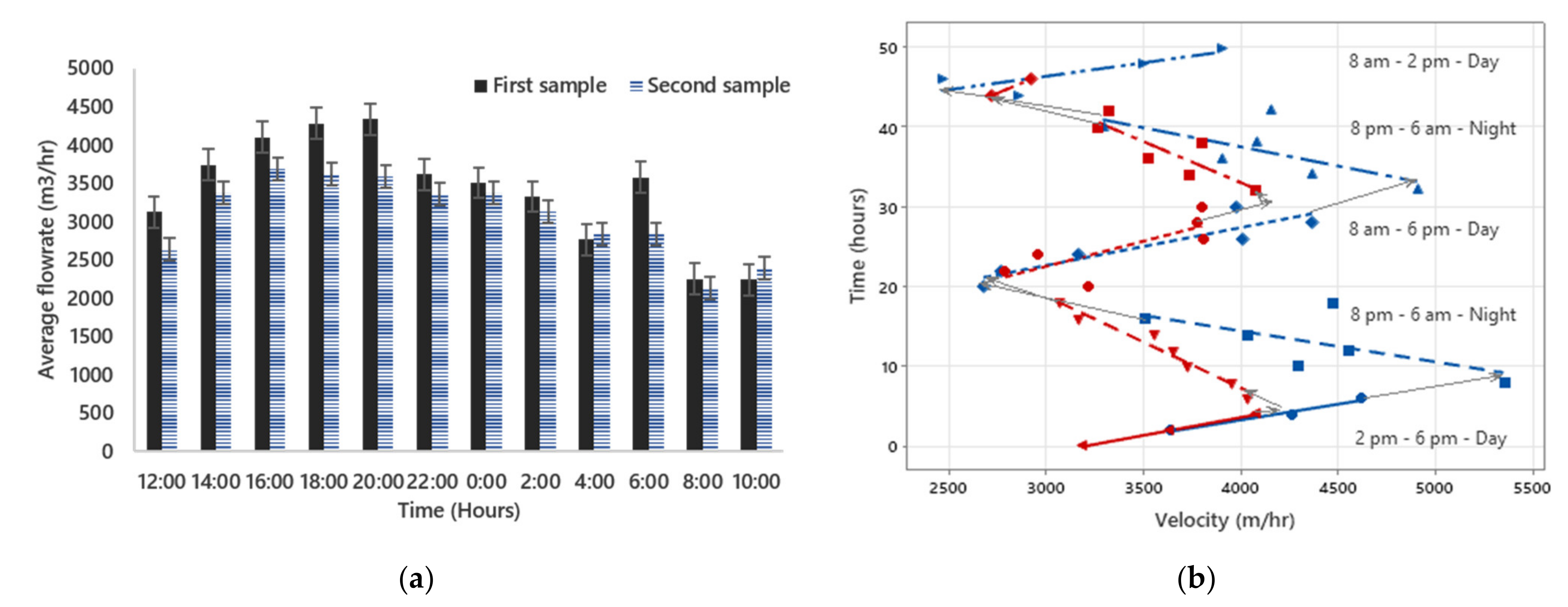
Wastewater quantity is expressed in terms of flowrate and velocity. Two sampling events were performed at the wastewater treatment plant. The flowrate of both events agrees mostly on the pattern; however, the first sample showed a higher magnitude than the second sample, as shown in Figure 1a. The first and second samples represent the average flowrate during the day and night of the first and second sampling events, respectively. During the sampling events, flowrates rose during the day to reach a maximum of 4338 m3/h and 3694 m3/h at around 8:00 p.m. in the first and second sampling events, respectively. Flowrate decreased during nighttime to reach the lowest of 2246 m3/h in the first sample and 2133 m3/h in the second sample at around 8:00 a.m. A spike in flowrate was observed at 6:00 a.m. for both sampling events. The percentage difference between the lowest and highest average flowrate is 48.2% and 42.2% in the first and second sampling events, respectively. The variation in flowrate was influenced by the working pattern of the inhabitants [34]. It was observed that flowrate and wastewater depth followed a similar pattern. Average wastewater depth was observed to be 0.8 m and maximum and minimum levels were 1.1 m and 0.7 m, respectively. In the first sampling event, H2S concentration was increasing steadily from 8:00 p.m. until it reached a peak value of 250 ppm at 4:00 a.m. H2S concentration then decreased to reach a minimum of 69 ppm at 8:00 p.m. However, on day 2 of the first sampling event, H2S concentration reached a peak several times. This pattern was not seen on any other sampling days. In the second sampling event, H2S concentration was at its peak (233 ppm and 280 ppm on day 1 and day 2, respectively) around 12:00 a.m. and at the lowest concentration (15 ppm and 13 ppm on day 1 and day 2, respectively) at 12:00 p.m. on both days.
It was observed that variation of velocity throughout the day had a diurnal pattern for both sampling events, as shown in Figure 1b. The scatter plot shows velocity in m/h on the x-axis against time in hours in increments of 10 on the y-axis. The blue symbols represent day 1 and day 2 of the first sampling event. The red symbols represent day 1 and day 2 of the second sampling event. The velocity shows high and low patterns within each day. Velocity is highest at 8:00 p.m. and lowest between 8:00 a.m. and 10:00 a.m. every day. In addition, the first sample had a wider range of velocity compared to the second sample. The variation in velocity with H2S had a cyclic pattern. This pattern was also repeated in the second sampling event. The first sampling event had a longer cyclic pattern because of the broader range of velocity. However, in terms of H2S concentration, the range was broader in the second sample. During the day of the first sampling event, there were higher H2S concentration values, resulting in an elevated cycle. The velocity decreased throughout the night and increased during the day for both samples. This resulted in a higher retention time at night, giving more time for the micro-organisms to convert sulfur-containing compounds to H2S. Hence, H2S concentration increased at night. An opposite phenomenon occurred during the day, as there was more volume of incoming wastewater, resulting in increased velocity. Both the cycles had 8:00 p.m. on one end and 8:00 a.m. on the other, depicting the beginning and end of the cycle. The highest point of the first and second cycles was at 4:00 a.m., where the H2S concentrations were 232 ppm for both cycles. The lowest point was different for both samples.
3.2. Wastewater Quality
The quality of wastewater was determined by studying the pH, COD, TSS, TDS, DO, temperature of wastewater, electrical conductivity, sulfide, chloride, total sulfur, TOC, and sulfate of wastewater. The maximum, minimum, and average values observed of each parameter are listed in Table 1. However, only pH, COD, sulfide, sulfate, and total sulfur exhibited a pertinent pattern throughout the sampling period. These variations are explained in detail in Section 3.4.
Sharma et al. [35] stated that solid sedimentation has a significant impact on H2S generation. The average TDS level was 491.7 ppm and maximum and minimum levels were 738 ppm and 323 ppm, respectively. The average TSS level was 160.4 ppm, and the maximum and minimum levels were 584 ppm and 73 ppm, respectively (Table 1). The level of dissolved oxygen in wastewater determines the amount of carbonaceous matter that can be broken down. An increase in DO level will result in lower sulfide generation by restricting the supply of food to the anaerobic bacteria [36]. However, a low DO level favors the generation of sulfide by enhancing the growth of anaerobic micro-organisms [36]. The typical DO level of wastewater is around 1 ppm [37]. In our case, the average DO level was 0.4 ppm and the maximum and minimum DO levels were 1.2 ppm and 0.05 ppm, respectively (Table 1).
A high temperature of wastewater is reported to increase biological activity and oxygen consumption. It also increases the sulfide generation in gravity sewers. The increase in temperature by one degree corresponds to a 7% increase in the activity of SRB until it reaches 30 °C [36]. It was observed that the temperature of wastewater is higher during the night, and lower during the day. This is because water has higher specific heat and it takes time to heat, hence temperature is lower during the day. The higher specific heat also prevents rapid temperature changes, and thus takes more time to cool at night [38]. The higher concentration of H2S during the night (between 12:00 a.m. and 6:00 a.m.) is in accordance with our discussion in the literature review that H2S concentration increases with increasing sewer temperature due to enhanced microbial activity with increasing temperature [39,40]. This pattern is similar for both sampling events. The average wastewater temperature was around 32.5 °C and the maximum and minimum were 31.8 °C and 32.7 °C, respectively (Table 1). The differences in wastewater temperature were not huge. Regardless of the temperature of headspace air, the wastewater temperature could not reflect the impact of the ambient temperature. Electrical conductivity (EC) has a significantly small effect on H2S in the aqueous phase [11]. According to US EPA [41], the effect of EC on H2S generation can be neglected. Average EC values were around 1271.9 µS/cm and maximum and minimum were 1929 µS/cm and 839.1 µS/cm, respectively (Table 1).
Total organic carbon (TOC) can be used as a type of substrate that SRB uses for its growth. Bacterial growth is aided by high quantities of organic materials. This results in the depletion of DO, which, in turn, enhances sulfide generation [36]. The average TOC was 306.3 ppm, and the maximum and minimum concentrations were 430.5 ppm and 215 ppm, respectively (Table 1). Chloride, along with other chemicals including ozone, hydrogen peroxide, permanganate, and oxygen, oxidizes sulfide directly [42]. Chloride also plays a role in facilitating the corrosion of steel by damaging its protective layer [43]. The average chloride level was 1098.2 ppm, and the maximum and minimum concentrations were 2281.2 ppm and 167.5 ppm, respectively (Table 1).
3.3. Effects of Different Parameters on H2S Emissions
3.3.1. Effect of Flowrate
Variations in flowrate and additional wastewater input have an effect on the release of odorant into the headspace [44]. Wastewater flowrate causes turbulence in the wastewater stream and increases or reduces re-aeration with high or low flow, respectively. It also determines the amount of sulfate entering the system [34]. In the case of H2S emissions, more wastewater results in an increased sulfate concentration. It was observed that flowrate and H2S concentration were negatively correlated for both sampling events. This is similar to the case of velocity, where a lower flowrate gives more time for micro-organisms to convert sulfate-containing compounds to H2S and release H2S gas to headspace. Generally, H2S concentration was higher during the night, with it being highest during the night of the second sampling event. During both the sampling events, H2S concentrations were at their maximum between 11:00 p.m. and 6:00 a.m. The flowrate varied between 2518.7 m3/h and 3524.8 m3/h during this time. H2S concentration was at its peak when the flowrate was around 3347 m3/h.
The variation in H2S concentration was limited during the first sampling event. However, during the second sampling event, the range was wider. In the case of flowrate, the variation was limited during the second sampling event; however, the range was broader during the first sampling event. Generally, H2S concentration was lowest during the day between 1:00 p.m. and 6:00 p.m., with it being the lowest during the day of the second sampling event. The flowrate varied between 3209.2 m3/h to 3925.9 m3/h during this period. During both sampling events, H2S concentration was at its lowest when the flowrate was around 3649 m3/h. There was a spike in H2S concentration between 11:00 p.m. and 12:00 a.m., and between 5:00 a.m. and 6:00 a.m. during a different flowrate range. An isolated dip was identified was in H2S concentration from 11:00 a.m. to 1:00 p.m. using contour plot analysis. The flowrate ranged between 2558.2 m3/h and 2716 m3/h during this event.
3.3.2. Effect of Sulfate Concentration
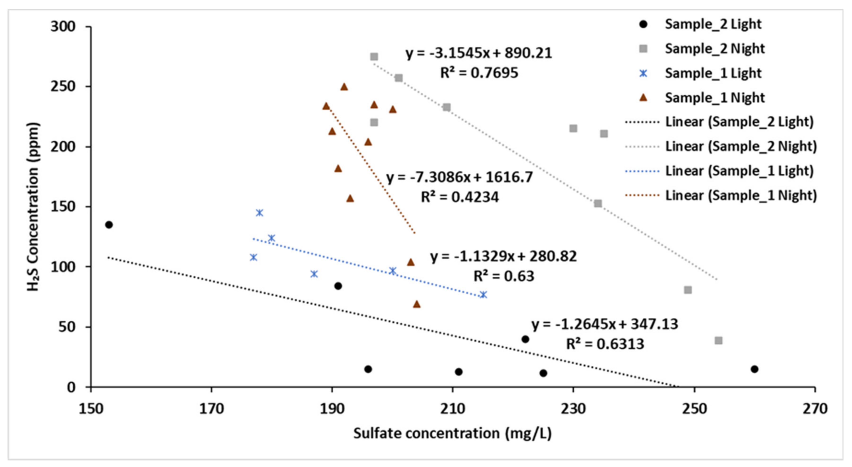
Hvitved et al. [45] stated that an increase in sulfate concentrations increases H2S generation since sulfate serves as the substrate in H2S production. The average sulfate concentration was 202.2 ppm, and the maximum and minimum concentrations were 260 ppm and 153 ppm, respectively (Table 1). The sulfate concentrations in the wastewater were higher during the night, as shown in Figure 2. The samples during the day and night of the first sampling event are represented as Sample_1 Light and Sample_1 Night, respectively. The samples during the day and night of the second sampling event are represented as Sample_2 Light and Sample_2 Night, respectively. Sulfate concentration ranged between 189 ppm and 200 ppm for the first sample and 196 ppm and 249 ppm for the second sample at night. H2S concentration was highest during this period (between 11:00 p.m. and 6:00 a.m.) for both samples. During the day, sulfate concentrations were lower. Sulfate concentration ranged between 177 ppm and 187 ppm for the first sample and 153 ppm and 196 ppm for the second sample during the day. H2S concentration was also lower during this period for both samples. However, there was a slight disruption to this pattern from 2:00 p.m. to 8:00 p.m. for the second sample. During this period, sulfate concentration was higher (between 210 ppm and 260 ppm), but H2S concentration was lower. It was observed that the flowrate was higher during this period. This reduced the retention time of the wastewater, thus reducing the amount of H2S released into the headspace. Hence, even at a higher sulfate concentration, the H2S concentration recorded was lower. Regression lines were developed for the sulfate concentrations of each sampling event, with separate regression equations for day and night. It was observed that although R-sq is low and does not justify correlation, H2S decreases with increasing sulfate concentration. The samples have the same R-sq value of 0.6 for daytime. However, the R-sq value of nighttime for the first sample is 0.4 and the second sample is 0.8.
It was observed that the variation in sulfate concentration with H2S had a cyclic, pattern as depicted. This pattern was repeated in the second sampling event. The second sampling event had a longer cyclic pattern, as the range of sulfate concentration was broader than in the first sampling event. Even in terms of H2S concentration, the range was broader in the second sampling event. Both cycles had 6:00 p.m. on one end and 10:00 a.m. on the other, depicting the beginning and end of the cycle. The lowest point of the first and second cycles was at 6:00 p.m., where the H2S concentrations were 77 ppm and 15 ppm, respectively. The highest point was different for both sampling events. The second sampling event had a longer cycle compared to the first sampling event. This is because the range of sulfate was wider in the second sampling event.
3.3.3. Effect of Sulfide
H2S gas is a byproduct of the dissociation of organic sulfide compounds [46]. Hence, the amount of sulfide available is important in determining the H2S emission. The average sulfide concentration was 0.1 ppm and the maximum and minimum concentrations were 0.3 ppm and 0.048 ppm, respectively (Table 1). H2S concentration varied at the same sulfide concentration for both sampling events. During the first sampling event, H2S concentration was higher between 10:00 p.m. and 8:00 a.m. However, at the same sulfide concentrations, H2S concentration was also lower between 10:00 a.m. and 8:00 p.m. During the second sampling event, H2S concentration was higher between 12:00 a.m. and 6:00 a.m. However, at the same sulfide concentration, H2S concentration was lower between 8:00 p.m. and 10:00 p.m. Between 12:00 p.m. and 4:00 p.m., H2S and sulfide concentrations were lower. However, between 4:00 p.m. and 8:00 p.m., H2S concentration was lower, even at higher sulfide concentrations. This can be explained by the variations in pH during the sampling events by considering the graph of equilibrium speciation of aqueous hydrogen sulfide as a function of pH [47]. At a lower pH, H2S concentration was higher, while at a higher pH, H2S was observed to be lower. This agrees with the observations made by Sharma et al., where pH and H2S concentration were correlated [37]. The pH of the wastewater sampling events collected in this study was between 6.9 and 7.2, at which there are equal chances of forming HS− and H2S [45].
3.3.4. Effect of Humidity
Humidity is one of the key factors leading to H2S-induced corrosion. Higher moisture content on sewer walls enhances microbial activity, which increases the rate of corrosion [48]. It was noted that humidity fluctuates together with H2S concentration, as shown in Figure S3 in Supplementary Materials. The first peak in H2S concentration coincides with the peak in humidity; however, humidity reaches a peak and stays constant for some time. The second peak in H2S has a pattern that is not similar to the peak in humidity. Neglecting the rapid changes in H2S concentration at the peak, H2S and humidity peaks can be considered coincidental. Both the peaks of H2S concentration during the second sampling event agree with the peaks of humidity. This is in agreement with the findings of Jiang et al., where it was concluded that when humidity increases, H2S concentration also increases [21].
3.3.5. Effect of Total Sulfur
Total sulfur is the sum of all sulfur-containing compounds present in both air and water. It was assumed that H2S from headspace and sulfide and sulfate from wastewater represent the majority of sulfur-containing compounds at a particular time. It was observed that the variation in total sulfur concentration in wastewater has a cyclic pattern. This pattern was repeated in the second sampling event. The first sampling event had a longer cyclic pattern. The range of total sulfur was broader in the first sampling event, resulting in a slightly erect cyclic pattern for the second sampling event. The highest point of the first and second cycles was at 6:00 a.m., where the total sulfur concentrations were 215 ppm and 306 ppm, respectively. The lowest point was different for both samples. This cyclic pattern was very similar to the patterns for flowrate and sulfate.
Total sulfur concentrations were higher during the night. During this period, total sulfur concentrations ranged between 260 ppm and 442 ppm for the first sampling event and 255 ppm and 458 ppm for the second sampling event. The flowrate was highest during this period for both sampling events. Regression lines were developed for total sulfur concentrations with the flowrate of each sampling event, with separate regression equations for day and night. The first and second sampling events had a similar R-sq value of 0.8 for nighttime. During the day, sulfate concentrations were lower. Sulfate concentration ranged from 180 ppm to 323 ppm for the first sampling event and from 283 ppm to 323 ppm for the second sampling event. The flowrate was also lower during this period for both sampling events. The R-sq value of the slope representing the daytime of the first sampling event is 0.7 and the second sampling event is 0.8.
It was noted that during nighttime, H2S concentration was higher. Total sulfur concentration was also higher during this period. H2S concentration during the day is comparatively lower, along with total sulfur concentration. This trend is similar for both the first and second sampling events. H2S concentrations were at their maximum between 10:00 p.m. and 8:00 a.m. The total sulfur concentration varied between 441 ppm and 364 ppm during this time. There was a spike in H2S concentration between 11:00 p.m. and 5:00 a.m., at a lower total sulfur concentration (between 219 ppm and 290 ppm). Neither flowrate nor pH was correlated with this increase in H2S concentration. However, the temperature of wastewater was highest during this period, which can explain the increase in H2S concentration. H2S concentration was lowest between 11:00 a.m. and 8:00 p.m., when the total sulfur concentration was in a lower range of between 188 ppm and 304 ppm.
3.3.6. Effect of pH
Dissociation of H2S to dissolved H2S gas, hydrogen sulfide ions, and sulfide ions is governed by the pH of wastewater [49]. Yongsiri et al. [11] stated that the pH of wastewater is important in evaluating H2S emissions. A decrease in pH is associated with increased H2S emissions, according to a study conducted by Nielsen et al. [50]. This agrees with our findings, where pH decreases while H2S concentration in the headspace increases, as shown in Figure S2 in Supplementary Materials. As discussed in the literature, pH determines the relative proportion between H2S and HS−. H2S concentration is favored at a lower pH. When the pH increases, the chances of H2S formation decrease, and HS− increases. The pH is low during the evening (from 12:00 p.m. to 10:00 p.m.) and quickly escalates to its highest value at 4:00 a.m. The pH values suddenly fall to reach their lowest at 10:00 a.m. and then rise rapidly again. This trend was evident for both the first and the second sampling events. The average pH value of the wastewater was 7.1, and the lowest and the highest values were 6.9 and 7.3, respectively (Table 1).
3.3.7. Effect of COD
COD has been reported as one of the influential factors in the generation of H2S in wastewater [40,45]. In the second sampling event, COD fluctuated with flowrate by a difference of 2 h. In the first sampling event, COD increased with increasing flowrate, but had a contrasting time difference compared to the second sampling event. This is contrary to the results reported by Wang et al., where COD decreased with increasing flowrate [51]. The authors had observed rainfall as a reason for the increase in flowrate. Hence, COD was reduced because of the dilution of the wastewater. In our case, when the flowrate increased, the amount of organic matter available also increased. Thus, COD increased with increasing flowrate. The average COD value of the wastewater for both days was 279.2 ppm, and the lowest and the highest values were 79.6 ppm and 546 ppm, respectively (Table 1).
3.4. Model for Prediction of H2S Emissions
Wastewater was collected from certain parts of the city, along with the wastewater collected in tankers were flowing through an enclosed structure. H2S concentration was measured in the headspace and sulfide and sulfate in the wastewater, with the assumption that no other forms of sulfur would be present to contribute to the total sulfur concentration. It was assumed that no H2S gas had escaped the system before the point of measurement. It was also assumed that the parameters that are not included in the study had little to no impact on H2S generation. The temperature of headspace, the temperature of wastewater, flowrate, wastewater depth, velocity of wastewater, moisture content, DO, COD, chloride, sulfates, sulfide, TSS, TDS, pH, electrical conductivity, TOC, and total sulfur were measured and analyzed. From the aforementioned parameters, significant parameters were identified using 95% significance in the correlation matrix. It was noted that the temperature of wastewater and the wastewater depth, total sulfur, and humidity were the significant factors influencing H2S generation, according to the collected data.
The data of the parameters selected to carry out the modeling were used in regression analysis. H2S concentration in ppm was taken as the response variable and the temperature of wastewater (TL) in °C, wastewater depth (WD) in m, total sulfur (TS) in ppm, and humidity (H) were continuous predictors. The analysis was performed at a 95% confidence level. The final regression equation obtained is shown in Equation (6):
From the model, it is evident that H2S concentration increases with increasing wastewater temperature, humidity, and total sulfur, and decreases with increasing wastewater depth. The model from regression had an R-sq value of around 0.7. This means that 74.3% of the variation in H2S concentration is explained by the parameters used in this model, as shown in Table 2.
The model developed in this study can serve as an important tool as it can be used for H2S control applications. The model can be improved by increasing the data collected. It can also help in understanding more layers of the variability of the parameters. However, this model is only applicable to the prediction of H2S in the particular treatment plant where the experiment was conducted. The model must be further developed for a more universal application. This is discussed in the next session.
3.5. Generalized H2S Emissions Prediction Model
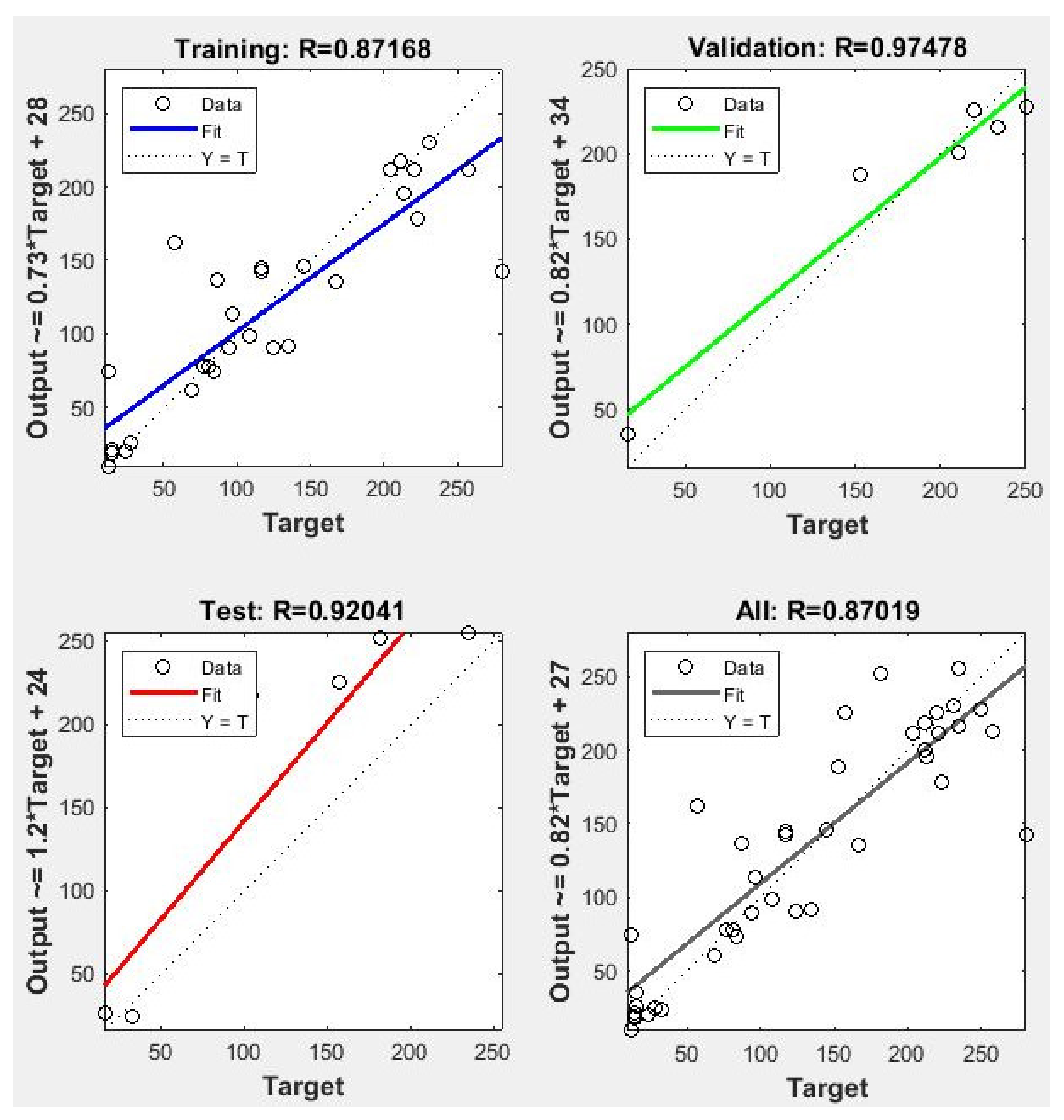
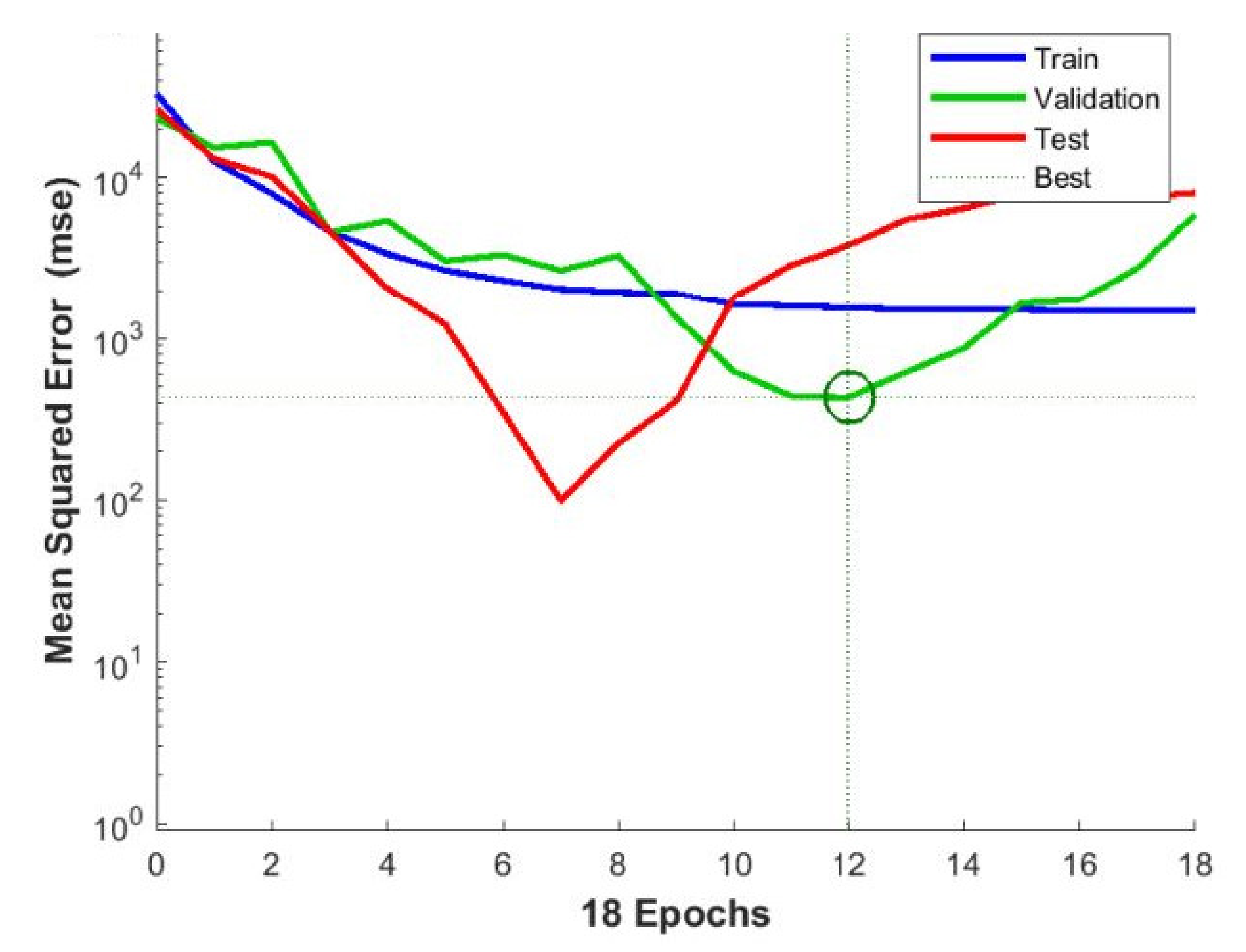
The regression model developed in Section 3.5 has limited applications because of its specificity. Hence, a neural net fitting application was used to analyze the dataset. Two variables were created in the workspace, which contains input data (parameters) and target data (H2S concentration) with four neurons in the hidden layers. The Levenberg–Marquardt backpropagation algorithm was used as the training algorithm. This algorithm gave the best results when compared to other training algorithm options in a short time (0:00:00). Out of the total 42 datasets, 30 were used for training, 6 for validation, and 6 for testing. The model obtained a good relationship from the training data, with an R value of 0.87, as shown in Figure 3. As proposed by Sivák et al. [52], an R-sq value of 0.9 or above is considered very good, and a value higher than 0.8 is good. An R-sq value of above 0.6 was considered acceptable. Thus, the data fit well with the model. The R values of validation and testing were 0.97 and 0.92, respectively. However, there are some probable outliers and scattering of the data. The best validation performance was obtained at an epoch of 12 (Figure 4). The prediction of the network is within 20% of the measured H2S concentration. This can be improved by increasing the data collection. In the study conducted by Rege et al. [33], a backpropagation algorithm was used to develop an ANN that could predict H2S emissions. They used a minimal quantity of data for model development, similar to this work. For some of the training data, the experimental error was reported to be in the order of 10%. There were errors in the emission rate estimations of up to 20%. Tian et al. [53] developed a two-phase mass transfer model based on the mass transfer rate equation for predicting H2S emissions. This model had an R-sq of 0.8714 between the predicted and measured concentrations of H2S, and they concluded that the model was reliable.
Additional tests were performed using this model. For testing, a dataset collected from another wastewater treatment plant was used. The network was tested using values of TL, WD, H, and TS as input data and H2S concentrations as target data. The R value of the performed test is 0.6, which can be considered acceptable. However, the low value of R is because the data was not collected from an input location, but at a buffer tank. This model did not consider other factors that might have an influence on H2S concentration. These include variations in VFAs, which are the most important carbon source for SRB [54] and BOD. Further, the dataset used in the model is limited to the location of data collection. Since artificial neural network (ANN) models are data-driven, the model can be improved by training with more data.
4. Conclusions
Microbial-induced concrete corrosion in sewers facilities is a consequential global concern incurring losses in the billions of dollars annually. This paper focuses on the generation of H2S gas in wastewater which is responsible for corroding concrete surfaces in wastewater treatment plants. This study examined the factors that affect the formation and generation of H2S in a wastewater treatment plant and formulated a model using the most important influencing parameters. The key findings are discussed in this section.
The variation of wastewater quantity throughout the sampling events is discussed. Sulfate and total sulfur concentration were observed to have a positive correlation with H2S concentration throughout the experimental period. The flowrate, velocity, sulfate, and total sulfur had a similar cyclic pattern throughout the sampling events. Sulfide concentrations were influenced by pH values since higher H2S concentrations were observed with higher and lower concentrations of sulfide. The effect of pH on H2S generation was studied. It was observed that higher H2S concentrations were recorded at lower pH values. The results also demonstrated that humidity and H2S concentration are positively correlated. The impact of other parameters like DO, COD, TOC, TSS, TDS, and temperature was also investigated. However, no clear patterns or correlations could be extracted from the data analysis.
The temperature of wastewater and its humidity, total sulfur, and depth were identified as the most important parameters influencing H2S emissions through correlation analysis. Based on the dataset collected from the inlet of the wastewater treatment plant, a statistical equation was proposed using regression analysis. However, due to the inapplicability of this model to any other wastewater treatment plant, a neural network model was developed. In the neural network model, validation and testing had an R value of 0.9. The training had an R value of 0.8. The model provided an accuracy of 80% for the prediction of H2S concentration in wastewater treatment plants. External environmental conditions impair the accuracy of prediction. The model was tested on a sample collected from the buffer tank of another wastewater treatment plant. The test had an R value of 0.6, indicating that the model is limited to its applicability in the prediction of H2S emissions under conditions similar to the inlet of a wastewater treatment plant. However, the model can be improved by training with more data.
Parameter analysis leads to the understanding of H2S emissions. This helps to manage H2S gas emissions in wastewater treatment plants, and, in turn, to control the bio-corrosion of concrete. In order to manage H2S emissions, it is necessary to know H2S emission patterns. Prediction tools are used in this situation, hence reducing the cost associated with H2S control measures. However, this model can be improved by analyzing more parameters, such as VFAs and biofilms. Since this model is data-driven, it can be further improved by increasing the collected data. By further developing this ANN model, it can be used for sewer modeling. Predictions of H2S emissions for large sewer and wastewater treatment plants can be developed by parametric emission modeling (PEM).
Supplementary Materials
The following supporting information can be downloaded at: https://www.mdpi.com/article/10.3390/w14050791/s1, Figure S1: Arial view of Al Saad wastewater treatment plant with the sampling area encircled. The arrow shows the direction of flow of wastewater in various treatment units; Figure S2: H2S concentration and pH levels at different times of measurements; Figure S3: H2S concentration and Humidity at different times of measurement.
Author Contributions
Conceptualization, A.A.H. and M.S.; methodology, A.A.H.; software, M.S.; validation, M.S.; formal analysis, A.A.H. and M.S.; investigation, A.A.H. and M.S.; resources, A.A.H.; data curation, M.S.; writing—original draft preparation, M.S.; writing—review and editing, A.A.H. and M.S.; visualization, M.S.; supervision, A.A.H.; project administration, A.A.H.; funding acquisition, A.A.H. All authors have read and agreed to the published version of the manuscript.
Funding
This research received no external funding.
Data Availability Statement
The data supporting the reported results can be made available by request to authors.
Acknowledgments
The authors extend their gratitude towards Mohammed Asad, Abdul Mannan Zafar, Manisha Kothari, Himadri Rajput, and Nisa Gopalan for reviewing the manuscript, and to Engineer Salem Hegazy for his assistance. The authors thank the personnel at Al Saad wastewater treatment plant and Corodex Trading for their cooperation.
Conflicts of Interest
The authors declare no conflict of interest. The funders had no role in the design of the study; in the collection, analyses, or interpretation of data; in the writing of the manuscript; or in the decision to publish the results.
References
- Boon, A.; Vincent, A. Odour generation and control. In Handbook of Water and Wastewater Microbiology; Elsevier: Amsterdam, The Netherlands, 2003; pp. 545–557. Available online: https://www.elsevier.com/books/handbook-of-water-and-wastewater-microbiology/mara/978-0-12-470100-7 (accessed on 17 January 2022).
- Talaiekhozani, A.; Bagheri, M.; Goli, A.; Khoozani, M.R.T. An overview of principles of odor production, emission, and control methods in wastewater collection and treatment systems. J. Environ. Manag. 2016, 170, 186–206. [Google Scholar] [CrossRef] [PubMed]
- Okabe, S.; Ito, T.; Sugita, K.; Satoh, H. Succession of Internal Sulfur Cycles and Sulfur-Oxidizing Bacterial Communities in Microaerophilic Wastewater Biofilms. Appl. Environ. Microbiol. 2005, 71, 2520–2529. [Google Scholar] [CrossRef] [PubMed] [Green Version]
- Liu, Y.; Zhou, X.; Shi, H. Sulfur Cycle by In Situ Analysis in the Sediment Biofilm of a Sewer System. J. Environ. Eng. 2016, 142, C4015011. [Google Scholar] [CrossRef]
- USEPA. Hydrogen Sulfide Corrosion: Its Consequences, Detection and Control. EPA 1991, 832S91100, 19. [Google Scholar]
- Wu, X.; Li, H.; Kan, Y.; Yin, B. A regeneratable and highly selective fluorescent probe for sulfide detection in aqueous solution. Dalton Trans. 2013, 42, 16302–16310. [Google Scholar] [CrossRef] [PubMed]
- De Belie, N.; Monteny, J.; Beeldens, A.; Vincke, E.; Van Gemert, D.; Verstraete, W. Experimental research and prediction of the effect of chemical and biogenic sulfuric acid on different types of commercially produced concrete sewer pipes. Cem. Concr. Res. 2004, 34, 2223–2236. [Google Scholar] [CrossRef]
- Jensen, H.S.; Lens, P.N.L.; Nielsen, J.L.; Bester, K.; Nielsen, A.H.; Hvitved-Jacobsen, T.; Vollertsen, J. Growth kinetics of hydrogen sulfide oxidizing bacteria in corroded concrete from sewers. J. Hazard. Mater. 2011, 189, 685–691. [Google Scholar] [CrossRef]
- Cwalina, B. Biodeterioration of concrete. Arch. Civ. Eng. Env. 2008, 4, 133–140. [Google Scholar]
- Davis, J.L.; Nica, D.; Shields, K.; Roberts, D.J. Analysis of concrete from corroded sewer pipe. Int. Biodeterior. Biodegrad. 1998, 42, 75–84. [Google Scholar] [CrossRef]
- Yongsiri, C.; Vollertsen, J.; Hvitved-Jacobsen, T. Effect of Temperature on Air-Water Transfer of Hydrogen Sulfide. J. Environ. Eng. 2004, 130, 104–109. [Google Scholar] [CrossRef]
- Gutierrez, O.; Park, D.; Sharma, K.R.; Yuan, Z. Effects of long-term pH elevation on the sulfate-reducing and methanogenic activities of anaerobic sewer biofilms. Water Res. 2009, 43, 2549–2557. [Google Scholar] [CrossRef] [PubMed]
- Nielsen, A.H.; Hvitved-Jacobsen, T.; Vollertsen, J. Effect of sewer headspace air-flow on hydrogen sulfide removal by corroding concrete surfaces. Water Environ. Res. 2012, 84, 265–273. [Google Scholar] [CrossRef] [PubMed]
- Zuo, Z.; Chang, J.; Lu, Z.; Wang, M.; Lin, Y.; Zheng, M.; Zhu, D.Z.; Yu, T.; Huang, X.; Liu, Y. Hydrogen sulfide generation and emission in urban sanitary sewer in China: What factor plays the critical role? Environ. Sci. Water Res. Technol. 2019, 5, 839–848. [Google Scholar] [CrossRef]
- Jiang, G.; Keller, J.; Bond, P.L. Determining the long-term effects of H2S concentration, relative humidity and air temperature on concrete sewer corrosion. Water Res. 2014, 65, 157–169. [Google Scholar] [CrossRef] [Green Version]
- Shypanski, A.H.; Yuan, Z.; Sharma, K. Influence of pressure main pumping frequency on sulfide formation rates in sanitary sewers. Environ. Sci. Water Res. Technol. 2018, 4, 403–410. [Google Scholar] [CrossRef]
- Yongsiri, C.; Vollertsen, J.; Rasmussen, M.; Hvitved-Jacobsen, T. Air-Water Transfer of Hydrogen Sulfide: An Approach for Application in Sewer Networks. Water Environ. Res. 2004, 76, 81–88. [Google Scholar] [CrossRef]
- Pomeroy, R.D.; Parkhurst, J.D. The forecasting of sulfide build-up rates in sewers. In Eighth International Conference on Water Pollution Research; Jenkins, S.H., Ed.; Elsevier: Pergamon, Turkey, 1978; pp. 621–628. [Google Scholar]
- Thistlethwayte, D.K.B.; Davy, W.J. The Control of Sulphides in Sewerage Systems; Butterworths: Sydney, Australia, 1972. [Google Scholar]
- Boon, A.G. Formation of sulphide in rising main sewers and its prevention by injection of oxygen. Prog. Wat. Tech. 1975, 7, 289–300. [Google Scholar]
- Haveman, S.A.; Greene, E.A.; Voordouw, G. Gene expression analysis of the mechanism of inhibition of Desulfovibrio vulgaris Hildenborough by nitrate-reducing, sulfide-oxidizing bacteria. Environ. Microbiol. 2005, 7, 1461–1465. [Google Scholar] [CrossRef]
- Tomar, M.; Abdullah, T.H. Evaluation of chemicals to control the generation of malodorous hydrogen sulfide in waste water. Water Res. 1994, 28, 2545–2552. [Google Scholar] [CrossRef]
- Bjerrum, J.; Schwarzenbach, G.; Sillen, L.G. Stability Constants of Metal-Ion Complexes, with Solubility Products of Inorganic Substances, Part I: Organic Ligands; Chemical Society: London, UK, 1957. [Google Scholar]
- Intrator, O.; Intrator, N. Interpreting neural-network results: A simulation study. Comput. Stat. Data Anal. 2001, 37, 373–393. [Google Scholar] [CrossRef] [Green Version]
- Braspenning, P.J.; Thuijsman, F.; Weijters, A.J.M.M. Artificial Neural Networks: An Introduction to ANN Theory and Practice; Springer Science & Business Media: Berlin/Heidelberg, Germany, 1995. [Google Scholar]
- Ebtehaj, I.; Bonakdari, H.; Zaji, A.H. A new hybrid decision tree method based on two artificial neural networks for predicting sediment transport in clean pipes. Alex. Eng. J. 2018, 57, 1783–1795. [Google Scholar] [CrossRef]
- Cheng, Z.; Li, X.; Bai, Y.; Li, C. Multi-Scale Fuzzy Inference System for Influent Characteristic Prediction of Wastewater Treatment. CLEAN Soil Air Water 2018, 46, 1700343. [Google Scholar] [CrossRef]
- Heo, S.; Nam, K.; Loy-Benitez, J.; Yoo, C. Data-Driven Hybrid Model for Forecasting Wastewater Influent Loads Based on Multimodal and Ensemble Deep Learning. IEEE Trans. Ind. Inform. 2020, 17, 6925–6934. [Google Scholar] [CrossRef]
- Yu, T.; Yang, S.; Bai, Y.; Gao, X.; Li, C. Inlet Water Quality Forecasting of Wastewater Treatment Based on Kernel Principal Component Analysis and an Extreme Learning Machine. Water 2018, 10, 873. [Google Scholar] [CrossRef] [Green Version]
- Boyd, G.; Na, D.; Li, Z.; Snowling, S.; Zhang, Q.; Zhou, P. Influent Forecasting for Wastewater Treatment Plants in North America. Sustainability 2019, 11, 1764. [Google Scholar] [CrossRef] [Green Version]
- Cheng, T.; Harrou, F.; Kadri, F.; Sun, Y.; Leiknes, T. Forecasting of Wastewater Treatment Plant Key Features Using Deep Learning-Based Models: A Case Study. IEEE Access 2020, 8, 184475–184485. [Google Scholar] [CrossRef]
- Kang, J.-H.; Song, J.; Yoo, S.S.; Lee, B.-J.; Ji, H.W. Prediction of Odor Concentration Emitted from Wastewater Treatment Plant Using an Artificial Neural Network (ANN). Atmosphere 2020, 11, 784. [Google Scholar] [CrossRef]
- Rege, M.A.; Tock, R.W. A Simple Neural Network for Estimating Emission Rates of Hydrogen Sulfide and Ammonia from Single Point Sources. J. Air Waste Manag. Assoc. 1996, 46, 953–962. [Google Scholar] [CrossRef]
- Nielsen, P.H.; Hvitved-Jacobsen, T. Effect of Sulfate and Organic Matter on the Hydrogen Sulfide Formation in Biofilms of Filled Sanitary Sewers. J. Water Pollut. Control Fed. 1988, 60, 627–634. [Google Scholar]
- Sharma, K.R.; Yuan, Z.; de Haas, D.; Hamilton, G.; Corrie, S.; Keller, J. Dynamics and dynamic modelling of H2S production in sewer systems. Water Res. 2008, 42, 2527–2538. [Google Scholar] [CrossRef]
- Sengupta, A. Preliminary Hydrogen Sulfide Emission Factors and Emission Models for Wastewater Treatment Plant Headworks. Ph.D. Thesis, University of New Orleans, New Orleans, LA, USA, 2014; p. 110. [Google Scholar]
- Nasr, M.; Moustafa, M. Performance evaluation of El-Agamy wastewater treatment plant—Egypt. In Proceedings of the 10th International Conference on the Role of Engineering Towards a Better Environment, Alexandria, Egypt, 15–17 December 2014. [Google Scholar]
- Faiman, D.; Hazan, H.; Laufer, I. Reducing the heat loss at night from solar water heaters of the integrated collector—Storage variety. Sol. Energy 2001, 71, 87–93. [Google Scholar] [CrossRef]
- Hvitved-Jacobsen, T.; Vollertsen, J.; Yongsiri, C.; Nielsen, A.; Abdul-Talib, S. Sewer microbial processes, emissions and impacts. In Proceedings of the 3rd International Conference on Sewer Processes and Networks, Paris, France, 15–17 April 2002. [Google Scholar]
- US EPA. Design Manual: Odor and Corrosion Control in Sanitary Sewerage Systems and Treatment Plants; U.S. Environmental Protection Agency: Washington, DC, USA.
- US EPA. Process Design Manual for Sulfide Control in Sanitary Sewerage Systems; US EPA: Washington, DC, USA, 1974.
- Neville, A. Chloride attack of reinforced concrete: An overview. Mater. Struct. 1995, 28, 63–70. [Google Scholar] [CrossRef]
- Cadena, F.; Peters, R.W. Evaluation of chemical oxidizers for hydrogen sulfide control. J. Water Pollut. Control Fed. 1988, 60, 1259–1263. [Google Scholar]
- Dincer, F.; Muezzinoglu, A. Odor Determination at Wastewater Collection Systems: Olfactometry versus H2S Analyses. CLEAN Soil Air Water 2007, 35, 565–570. [Google Scholar] [CrossRef]
- Hvitved-Jacobsen, T. Sewer Processes: Microbial and Chemical Process Engineering of Sewer Networks; CRC Press: Boca Raton, FL, USA, 2001. [Google Scholar]
- Yalamanchili, C.; Smith, M.D. Acute hydrogen sulfide toxicity due to sewer gas exposure. Am. J. Emerg. Med. 2008, 26, 518.e5–518.e7. [Google Scholar] [CrossRef] [PubMed]
- House, M.; Weiss, W.J. Review of Microbially Induced Corrosion and Comments on Needs Related to Testing Procedures. In Proceedings of the 4th International Conference on the Durability of Concrete Structures, West Lafayette, IN, USA, 24–26 July 2014; pp. 94–103. [Google Scholar] [CrossRef] [Green Version]
- Mori, T.; Nonaka, T.; Tazaki, K.; Koga, M.; Hikosaka, Y.; Noda, S. Interactions of nutrients, moisture and pH on microbial corrosion of concrete sewer pipes. Water Res. 1992, 26, 29–37. [Google Scholar] [CrossRef]
- Geraghty, P.J. Ireland’s environmental protection agency act 1992: An overview. Eur. Environ. 1993, 3, 10–13. [Google Scholar] [CrossRef]
- Nielsen, A.H.; Vollertsen, J.; Jensen, H.S.; Madsen, H.I.; Hvitved-Jacobsen, T. Aerobic and Anaerobic Transformations of Sulfide in a Sewer System-Field Study and Model Simulations. Water Environ. Res. 2008, 80, 16–25. [Google Scholar] [CrossRef]
- Wang, M. Network Modelling of the Formation and Fate of Hydrogen Sulfide and Methane in Sewer Systems. Ph.D. Thesis, University of Sheffield, Sheffield, UK, 2017. [Google Scholar]
- Sivák, P.; Ostertagová, E. Evaluation of Fatigue Tests by Means of Mathematical Statistics. Procedia Eng. 2012, 48, 636–642. [Google Scholar] [CrossRef] [Green Version]
- Tian, L.; Han, C.; Zhang, J.; Ouyang, Y.; Xi, J. Development of an H2S emission model for wastewater treatment plants. J. Air Waste Manag. Assoc. 2021, 71, 1303–1311. [Google Scholar] [CrossRef]
- Gu, T.; Jia, R.; Unsal, T.; Xu, D. Toward a better understanding of microbiologically influenced corrosion caused by sulfate reducing bacteria. J. Mater. Sci. Technol. 2018, 35, 631–636. [Google Scholar] [CrossRef]
Figure 1.
Variation of wastewater quantity throughout the sampling event. (a) Average flowrate during the first and second sampling events. (b) Scatterplot showing the velocity of wastewater at different times of the day.
Figure 1.
Variation of wastewater quantity throughout the sampling event. (a) Average flowrate during the first and second sampling events. (b) Scatterplot showing the velocity of wastewater at different times of the day.

Figure 2.
Comparison between H2S concentration and sulfate concentration during the day and night of the first and second sampling events.
Figure 2.
Comparison between H2S concentration and sulfate concentration during the day and night of the first and second sampling events.

Figure 3.
Outputs of the model using training, validation, testing, and overall datasets.

Figure 4.
Performance of the neural network showing MSE.


Table 1.
The maximum, minimum, and average values of wastewater characteristics.
| Parameter | Maximum Value | Minimum Value | Average |
|---|---|---|---|
| pH | 7.3 | 6.9 | 7.1 |
| COD (ppm) | 546 | 79.6 | 279.2 |
| TOC (ppm) | 430.5 | 215 | 306.3 |
| DO (ppm) | 1.2 | 0.05 | 0.5 |
| Temperature of wastewater (°C) | 32.7 | 31.8 | 32.5 |
| Temperature of air (°C) | 42 | 32 | 35.5 |
| EC (µS/cm) | 1929 | 839.1 | 1271.9 |
| Sulfate (ppm) | 260 | 153 | 202 |
| TDS (ppm) | 738 | 323 | 491.7 |
| TSS (ppm) | 584 | 73 | 160.4 |
| Sulfide (ppm) | 0.4 | 0.05 | 0.1 |
| Chloride (ppm) | 2281.2 | 167.5 | 1098.2 |
Table 2.
Summary of the regression model.
| Model Summary | |||
|---|---|---|---|
| S | R-sq | R-sq (adj) | R-sq (pred) |
| 45.6328 | 74.38% | 71.08% | 62.41% |
Publisher’s Note: MDPI stays neutral with regard to jurisdictional claims in published maps and institutional affiliations. |
© 2022 by the authors. Licensee MDPI, Basel, Switzerland. This article is an open access article distributed under the terms and conditions of the Creative Commons Attribution (CC BY) license (https://creativecommons.org/licenses/by/4.0/).
Share and Cite
MDPI and ACS Style
Sherief, M.; Aly Hassan, A. The Impact of Wastewater Quality and Flow Characteristics on H2S Emissions Generation: Statistical Correlations and an Artificial Neural Network Model. Water 2022, 14, 791. https://doi.org/10.3390/w14050791
AMA Style
Sherief M, Aly Hassan A. The Impact of Wastewater Quality and Flow Characteristics on H2S Emissions Generation: Statistical Correlations and an Artificial Neural Network Model. Water. 2022; 14(5):791. https://doi.org/10.3390/w14050791
Chicago/Turabian StyleSherief, Mohsina, and Ashraf Aly Hassan. 2022. "The Impact of Wastewater Quality and Flow Characteristics on H2S Emissions Generation: Statistical Correlations and an Artificial Neural Network Model" Water 14, no. 5: 791. https://doi.org/10.3390/w14050791
Note that from the first issue of 2016, this journal uses article numbers instead of page numbers. See further details here.