
Application of the British Columbia MetPortal for Estimation of Probable Maximum Precipitation and Probable Maximum Flood for a Coastal Watershed


Hydrotechnical Engineering, BC Hydro, Burnaby, BC V3N 4X8, Canada
*
Authors to whom correspondence should be addressed.
Water 2022, 14(5), 785; https://doi.org/10.3390/w14050785
Submission received: 31 January 2022
/
Revised: 24 February 2022
/
Accepted: 28 February 2022
/
Published: 2 March 2022
(This article belongs to the Special Issue Advances in Flood Forecasting and Hydrological Modeling)
Abstract
:Estimation of the Probable Maximum Precipitation (PMP) and Probable Maximum Flood (PMF) are regulatory requirements in many jurisdictions that are used in the design of dams and assessment of existing infrastructure. The recently available British Columbia MetPortal provides regionally consistent PMP and precipitation frequency estimates across the province of British Columbia (BC). This paper proposes an approach to process and apply this data for the estimation of the PMF for watersheds across British Columbia. Guidelines are presented for selection of transposition points applicable to a watershed, and algorithms are developed for processing the geospatial probable maximum storm and precipitation frequency data. The algorithms developed are generic to multiple software and programming environments, and could also be applied in other regions where spatially and temporally intact PMP estimates are available. A detailed description of data sources and development of PMF scenario inputs is provided, as well as details of important sensitivity analyses. The methodology is applied to estimate the PMF for the Cheakamus Basin north of Squamish British Columbia. The application of the MetPortal PMP and precipitation frequency estimates, when used with a consistent PMF development methodology as proposed in this paper, will help improve the consistency of PMF estimates for watersheds across the province, offering a welcome improvement for dam owners and regulators.
1. Introduction
The Probable Maximum Flood (PMF) is the theoretical maximum flood that can reasonably be expected to occur for a given location. It is derived based on the Probable Maximum Precipitation (PMP) or Probable Maximum Snow Accumulation (PMSA), in combination with other conditions—for example a precipitation event, snowpack or temperature sequence—not exceeding a 1/100 year Annual Exceedance Probability (AEP) [1]. Generally, a number of combinations of antecedent conditions and timing are tested to estimate the most severe possible flood.
In the province of British Columbia (BC), Canada, the regulation and design of dams is based on their failure consequence, as determined by guidelines developed by the Canadian Dam Association (CDA), which recommends target levels for flood withstand based on the consequence classification of the dam [1]. In the CDA-recommended standards-based approach to flood hazard, the PMF is used in the determination of target standards from High to Extreme consequence dams. The PMF is also a regulatory requirement or recommendation in many other jurisdictions (including but not limited to: Brazil, India, Turkey, Norway, New Zealand, the United States, and the United Kingdom [2]). Despite its widespread use, there are a number of known issues with the PMP/PMF approach, described in detail in [3]. There are many methods available to compute the PMP, which can result in large discrepancies in PMP/PMF estimates computed for the same watershed [3], creating further challenges for dam owners in assessing a dam’s adequacy with respect to flood passage. PMP and PMF are by nature deterministic assessments of flood loading and do not provide the probabilistic information useful in analyzing dam risk [4]. Newer approaches relying on stochastic simulation have recently been gaining momentum within the dams community (e.g., [4]), and risk-informed approaches to dam safety involving probabilistic flood estimates are becoming more common in various jurisdictions as the science evolves [5]. However, given that there remains a high prevalence of the PMP/PMF concepts within the regulatory frameworks of many jurisdictions, the need for these estimates is likely to remain for the foreseeable future. Therefore, improvements in PMP and PMF estimation methods are still important and warranted.
This paper provides a detailed description of the application of the new BC MetPortal tool with regional PMP and precipitation frequency estimates to estimate the PMF of a coastal watershed in British Columbia, Canada. One of the key advantages of the new BC MetPortal approach is that it provides regionally consistent estimates of the PMP, generated from the same methodology, using the same storm database and created by the same analysts. This has the potential to significantly improve consistency among PMF estimates for various facilities across British Columbia.
A new methodology is presented for processing the data available from the BC MetPortal to generate PMF estimates for dams in British Columbia. The methods presented in this paper are also applicable for PMF estimation in other regions where spatially and temporally intact PMP estimates are available. Enhanced geospatial processing capabilities have made this style of PMP estimate more widely available in recent years. Much of the existing guidance material on PMF estimation pertains to the use of PMP estimates derived by storm separation and applied to watersheds using depth-area-duration curves. This paper aims to provide guidance on preserving the spatial and temporal characteristics of the PMP in hydrological model forcings, and provides additional discussion of model inputs and sensitivity analyses.
The remainder of the introduction provides a background of pertinent concepts associated with estimation of the PMP and PMF, an overview of the BC Extreme Flood Project and the data available within the BC MetPortal, and a description of the study area. In the following section, a detailed description of the approach for applying the BC MetPortal PMP and precipitation frequency estimates to a specific watershed for PMF estimation is presented. The Results section provides the detailed case study for the Cheakamus Dam in BC, Canada, and is followed by a discussion.
1.1. Probable Maximum Precipitation
The World Meteorological Organization (WMO) defines the PMP as “the theoretical maximum precipitation for a given duration under modern meteorological conditions. Such a precipitation is likely to happen over a design watershed, or a storm area of a given size, at a certain time of year” [6]. There are a number of methods available with which to develop estimates of the PMP, which are summarized in [6]. The two major methods for PMP analysis are:
- Statistical methods, which develop PMP estimates based on historically recorded annual maxima at locations of interest. The statistical method is a convenient and simple way to estimate the PMP but is generally no longer used and has been replaced with the meteorological methods that are more common [7].
- Meteorological methods, which involve the use of observed precipitation from historical storms, are moisture-maximized and transposed to the area of interest. Meteorological methods can take a number of forms that are described in more detail in [6].
The standard approach (e.g., Generalized Method) for transposing storms involves separating the storm into orographic and convergence components, as well as summarizing storm precipitation into a Depth-Area-Duration (DAD) table and moving the DAD table of a particular storm to the location of interest [8]. This approach provides an elementary analytical summary of storm depths by area size and duration to which moisture and orographic factors could be applied. However, the DAD table fails to maintain spatial and temporal patterns, which are imperative to simulating real storms and modelling floods. According to [9], consideration of the storms as intact, using storm transposition as outlined in [6], is scientifically preferable to separating the storms into components, or decomposing the storms into depth-area-duration tables, as these approaches tend to lose the spatial and temporal characteristics of real-world storm events.
As summarized in [10], the Enhanced Storm Transposition Procedure (ESTP) is a new approach that builds on the WMO’s storm transposition method, by leveraging precipitation-frequency statistics, inherently encompassing and accounting for the underlying moisture availability, topography, meteorology, and climatology between the in-place storm location and the design watershed/location. The ESTP begins by in-place maximization of the observed storm precipitation. Once the critical maximum storm precipitation duration is identified (e.g., 48-h, 72-h, 96-h, etc.) an accumulation grid is computed. The precipitation frequency grids for the identified duration are used to translate the precipitation in-place, at each gridcell, into an equivalent annual exceedance probability (AEP). The gridcell with the rarest precipitation frequency is identified, which represents the storm center and location of greatest storm efficiency (i.e., the transformation of water vapor to precipitation on the ground). There may be multiple, distinct storm centers for a given storm [9]. The transposition limits are identified as well as what in-place maximization factor would be applied to maximize the moisture within the storm. The storm centers relevant to a transposition point of interest are then transposed to the selected point design location and mapped back to precipitation using the precipitation frequency grids at the design location.
Each storm, once moisture-maximized and transposed using the ESTP, can be analyzed for its potential to control the PMP at the design location. The Probable Maximum Storm (PMS) is the storm that controls the PMP, which is determined by computing the maximum areal average precipitation volume occurring over the specified duration and area size. Of all transposed storms, the storm with the greatest areal average precipitation for a specified area and duration is the PMS. The PMP is equal to the maximum areal average precipitation produced by the PMS over the basin area [11]. It is important to note that the interplay of spatial and temporal characteristics of storm precipitation could also potentially result in a storm with a lower areal volume of precipitation controlling the PMF within a watershed.
1.2. Probable Maximum Flood
Development of PMF estimates for watersheds across Canada generally follows the approach described in the CDA Dam Safety Guidelines [1] which is briefly summarized here and expanded upon as required for context.
The first step in computing the PMF is to determine the PMP, as well as its uncertainty bounds and seasonal adjustment factors. Dewpoint temperatures for the storm event being simulated should also be derived, if possible, otherwise conservative assumptions for temperature sequences and lapse rates during the PMP can be made. Next, rainfall, temperature and snow-accumulation statistics over the basin are calculated, and can be based on gauged information or regional analysis. Frequency analysis of precipitation, temperature and snowpack are used as inputs to various PMF scenarios. A rainfall-runoff model is another required input for PMF modelling, and calibration of this is carried out using historic rainfall and runoff data for the watershed of interest. Where possible, the largest floods on record and rain-on-snow events should be used in model calibration to ensure verification of the model under the extreme conditions characteristic of major floods. Initial conditions are input to the rainfall-runoff model that should ensure soil moisture is maximized prior to the onset of the PMP. This can be achieved by simulation of a 1:100-year pre-storm event prior to the PMP. Extreme temperature sequences to ripen snowpack may also be considered in some cases. The PMF is then computed using the rainfall-runoff model with the previously established PMP and the initial conditions pertinent to the scenario of interest.
Typically, two PMFs are computed, depending on the basin geography and location. These are (a) a summer–autumn PMF, which is generated by a seasonal PMP, and (b) a Spring PMF that is contributed to significantly by snowmelt and is generally either a spring PMP and snowpack with a 1:100-year frequency, or the PMSA with a 1:100-year frequency rain event [1]. However, depending on the basin location and geography, there may be characteristics that warrant the investigation of other PMF scenarios that could potentially govern the maximum flows in the watershed.
1.3. British Columbia Extreme Flood Project
The British Columbia Extreme Flood Project is a comprehensive study of province-wide PMP and precipitation frequency estimates, completed in 2020 and initiated by the provincial government of British Columbia. The products of this study are available online on the BC MetPortal [12], as are a detailed user guide [9] and technical manual [11]. The MetPortal provides gridded estimates of the PMP at a set of specific points for selected basin area sizes (ranging from 10 km2 to 10,000 km2) and durations (24, 48, 72 and 96-h durations). PMP estimates were derived using the Enhanced Storm Transposition Procedure (ESTP) and storm maximization, as described above.
For the BC Extreme Flood Project, a total of 44 storms with 82 distinct storm centers were reconstructed spatially and temporally using MetStorm, a GIS-based software and observed gauge information [9]. Details of each individual storm analysis are summarized in MetStorm Reports, available on MetPortal. The PMS was provided at the 24-, 48-, 72-, and 96-h durations and for watershed areas ranging from 1 km2 to 10,000 km2 for all transposition points across BC. To determine the PMS, the areal average precipitation for each transposed storm was computed for a square box with an area equal to the specified area size, centered on each transposition point. The PMS is the storm that has the greatest precipitation volume over the duration and area size of interest (note that the PMS is derived from a real event that may have durations longer than the PMP duration of interest—a rolling window is used to determine the maximum over the period of interest). The PMS includes the storm spatial and temporal patterns (maximized then transposed using the ESTP) as hourly grids, as well as associated dewpoint temperatures and freezing levels for the storm duration. The analysis by DTN also provides seasonality factors, indicating what percentage of the PMP would be possible within a given month and “macro-region”.
Uncertainty analysis was used to develop scaling multipliers for each macro-region for the 5th percentile, median and 95th percentile PMP estimates, as determined following the Monte Carlo approach presented in [7] and described in detail for the BC Extreme Flood Project application in [11]. These multipliers are useful for increasing the level of conservatism in the deterministically derived PMP estimates. The multipliers provided for each macro region for the 5th, median and 95th percentile values are all greater than 1—this situation occurs because there are sizable uncertainties in the inputs/factors used in estimating PMP that could result in plausible PMP values significantly greater than those computed deterministically.
In addition to the PMP estimates at transposition points across the province, the MetPortal also provides regional precipitation frequency analysis results in raster format and for point locations for particular storm durations. Five different temporal patterns are provided by DTN that can be used to scale the precipitation frequency estimates to generate realistic, spatio-temporal storm inputs at various frequencies and durations [9]. For the regional precipitation frequency analysis, which used the methodology described in [13], gauged precipitation observations from across the province and extending into the northwestern United States were used to compute magnitude-frequency relationships, gridded across the entire province using regional L-moment statistics.
2. Materials and Methods
2.1. Development of PMP
The MetPortal provides spatio-temporal data from the specific Probable Maximum Storm (PMS) that produced the PMP for a given transposition point. PMS’s are derived from geospatial reconstructions of real storms, which have been moisture-maximized and transposed to various transposition points across the province of British Columbia, for different watershed areas and durations of interest. To assess the applicability of transposition point PMS data in development of the PMP for a watershed, the PMS data from the nearby and/or in-basin transposition points should be analyzed by determining the basin average PMP—this value will differ from the PMP estimates provided by MetPortal because it is computed using the basin geometry and area, whereas MetPortal PMP estimates are computed for a square box centered on the transposition point.
The PMS data file for a given transposition point, PMP duration and basin-area size contain hourly spatial precipitation grids as well as grids of total storm precipitation. Both of these should be consulted to assess the suitability of the transposition point for computation of the PMP in the basin. An area size close to the basin area should be selected for the analysis. Because the PMP is based on a real storm often lasting over 100 h and there may be several transposition points and PMS storms to assess, there are a large number of hourly precipitation grids to analyze.
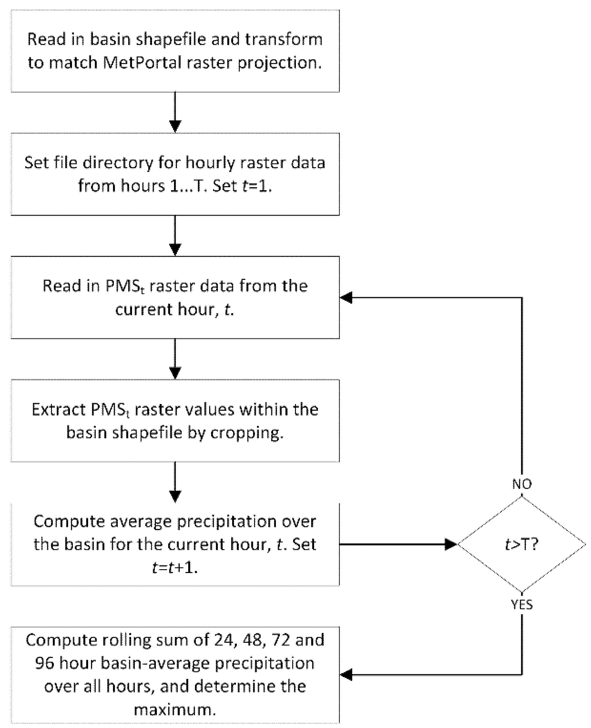
To analyze the data from the MetPortal, a Python script was developed to automatically analyze the geospatial data and determine basin average precipitation for a given PMS from a given transposition point, duration and area size. Automated processing of the hourly spatial precipitation totals is the most efficient approach to analyze the many iterations required for different transposition points, durations and basin areas. The program follows the flow chart shown in Figure 1. The Python script uses a number of open-source packages including numpy, rasterio, geopandas and shapely. The general program flow shown in Figure 2 is also applicable within GIS or other programming languages.
Following calculation of basin average precipitation for various durations and transposition points, a comparison should be made between the various transposition points to assess whether they produce similar basin average PMPs or have significant variation. Significant variation may occur when the precipitation footprint of the storm is in a narrow band or oriented in some way that avoids the watershed area. Depending on the area analyzed, the PMS storms for different transposition points may also be produced by different historical events. Visualization of the storm total precipitation is helpful to analyze the precipitation footprint and determine whether it appears that precipitation is maximized within the basin, or whether additional transposition may be required. In some cases, the orientation of the precipitation footprint at nearby transposition points may not maximize precipitation within the basin boundary. Due to orographic considerations during storm transposition (which have a significant impact in mountainous areas of British Columbia), it is not advisable to shift storm grids such that the precipitation is centered over the basin [9]. Custom transpositions may be required in this case.
2.2. Development of PMF
To simulate the most severe combination of snowpack, antecedent conditions, temperatures and precipitation, a number of different PMF scenarios are generated and run using a hydrologic model. The scenarios combine the various elements in a number of ways to determine the most severe combination. This section provides an overview of the various inputs for hydrologic modelling of the PMF. Note that PMSA is not discussed here and can be generated using common methods such as those described in [14].
In this study, the Raven hydrological modelling framework [15] is used with the UBC Watershed Model emulation [16,17]. In Raven, the watershed is divided into Hydrological Response Units (HRUs), which are based on elevation bands (from the UBC Watershed Model), further discretized based on slope aspect and land cover. In order to run the hydrologic model for PMF simulation and preserve the spatial and temporal aspects of the PMS, as provided by the MetPortal, distinct inputs are generated for each HRU from the storm’s hourly raster data, as well as temperature and snowpack inputs. The methodology for development of these inputs is described in this section.
2.2.1. PMP and 100-Year Pre-Storm
To generate hydrological model forcings that preserve the spatial and temporal characteristics of the storm, the PMS raster data is processed for each hydrologic response unit. The approach developed within Python and presented in Figure 1 is extended using shapefiles for each HRU in the watershed, as shown in Figure 2. Automated processing allows efficient generation of hydrological model forcings for many hourly files and iterations of transposition points, durations and basin sizes. It is important to consider the resolution of the PMS raster data in comparison with the resolution of the HRU shapefiles. GIS and Python spatial averaging and cropping tools only consider raster grids with a center point within the geometry of the shapefile. In some cases, this may limit the amount of data considered in the calculation of the spatial average. Reprojection of the PMS raster data may be required to generate the true average of the raster data within the HRU polygons. Again, the approach presented in Figure 2 is generalized and could be applied within the GIS framework, or in other programming languages, and could be applied to any temporally and spatially preserved storm data to generate hydrological model forcings.
Another important consideration in PMF simulation is the generation of antecedent conditions that maximize the soil moisture within the watershed prior to the onset of the PMP. It is recommended that a pre-storm not exceeding 1 in 100-year AEP precipitation event is used for this purpose, though critical temperature sequences and snowmelt may also produce extreme soil moisture and should also be considered. The BC MetPortal provides point precipitation-frequency estimates across the province of BC, estimated using regional precipitation frequency analysis with the methodology described in [13]. These can be used, along with Areal Reduction Factors (ARFs) and spatio-temporal patterns based on real storms (either the PMS or other temporal sequences as available in MetPortal) to generate a realistic 100-year pre-storm for the basin of interest.
The basin average point-precipitation can be generated from the MetPortal precipitation frequency raster data for a given duration using the same steps as shown in Figure 1. The basin’s average point-precipitation must be multiplied by an ARF to ensure reasonable precipitation distribution across the basin (it is not reasonable to have a 100-year event occurring simultaneously at every point across the basin at the same time). ARFs are most important for watersheds greater than about 25 km2 in size; otherwise, ARFs can be assumed to be negligible.
The original and broadly accepted calculation method for ARF values, proposed by the U.S. Weather Bureau in 1958, is to divide the basin average annual maximum precipitation by the maximum point precipitation value [18]. Attempts were made by the U.S. Weather Bureau to produce recommendations on acceptable ARF values [19,20]. These are still widely used today, despite significant additional data having become available and a number of studies suggesting that ARF values could vary significantly by storm type and between basins based on region and climate [21,22]. These and other more recently proposed calculation methods for ARF (such as those described by [22]) are known as “geographically fixed” and most applicable to precipitation frequency analyses.
Storm-centered ARF calculations are most applicable for PMP applications but can also be used as a proxy when geographically fixed ARF values are not available. The storm-centered approach calculates ARF values for several observed and reconstructed storms (prior to any maximization and transposition), to generate a best-estimate ARF for a storm type. These are readily available as part of the Depth-Area-Duration analysis of a detailed storm precipitation analyses. The calculation method is similar to that proposed by [18]; however, instead of gauged precipitation, reconstructed storm grids are used and a comparison between the basin average and the storm maximum cell (or cells) is computed.
When applying the spatio-temporal patterns of the PMS to the 100-year storm, the basin average PMP for the selected duration is used to scale the precipitation amounts in each HRU—by dividing the hourly precipitation values in each HRU by the basin average PMP. The ARF-adjusted basin average 100-year point precipitation is then multiplied into these scaling factors, to generate a spatially and temporally realistic 100-year storm pattern for hydrologic modelling input.
2.2.2. Temperatures
A variety of different temperature inputs are required for modelling of the various PMF scenarios, which are developed using observed temperatures from within or near the basin and, where necessary, frequency analysis.
For PMP storm temperatures, the BC MetPortal provides 1000 mb temperatures and freezing levels for each PMS, at the location of the original, non-transposed storm center. These can be adjusted to the mean elevation of each HRU using an assumed lapse rate. The pseudo-adiabatic lapse rate recommended by [23] is 5 °C per 1000 m elevation gain. In mountainous regions, this may not be sufficient to ensure that the majority of precipitation, including in the upper elevations of the basin, is falling as rain. The assumed lapse rate may be adjusted lower to increase the percentage of the PMP that falls as rain within the higher elevation HRUs. Similar to PMP storm temperatures, the 100-year pre-storm developed using the point-precipitation frequency grids from the MetPortal can apply the 1000 mb temperatures from the storm used to scale the ARF-adjusted basin average precipitation—whether that be the PMS or one of the storms provided within the Temporal Patterns tab of the MetPortal.
In the PMF scenarios, average dry transition days are also required—in between the pre-storm and the PMP, and also after the PMP to allow the simulation of PMF recession. These can be generated by calculating the historically observed average maximum temperatures for the month of interest and applying the average hourly diurnal temperature relationships for the month and climate station. Lapse rates can then be applied to determine temperature inputs for the average dry transition days at each HRU.
Finally, in lieu of a 100-year pre-storm, critical snowmelt temperature sequences may be applied to simulate extreme snowmelt conditions as an alternative antecedent condition prior to the onset of the PMP. The critical temperature sequence promotes the ripening of the snowpack and creates excessive soil moisture that may have the potential to generate severe flows under the seasonally adjusted PMP or the 100-year storm. These can be derived from the observed maximum temperature data using frequency analysis. To generate a critical temperature sequence, the annual maximum cumulative temperatures at 1, 2, 3, 5, 10, and 15-day windows ending on the PMP start day of interest are calculated. Frequency analysis software can be used to generate 100-year values from the observed data. A variety of extreme-value distributions and fitting methods should be applied to determine the best fit and assess conservatism in the estimated 100-year values.
A 15-day 100-year daily maximum temperature sequence is generated from the 100-year cumulative temperatures, assuming the maximum daily temperatures over the 15-day period have an increasing trend. The cumulative values from the shorter sequences are imbedded within the longer sequences and values in-filled using interpolation. Daily maximum temperatures are then organized from lowest to highest in the 15-day sequence. To generate hourly data from the 15-day maximum temperature sequence, the average observed diurnal patterns are applied to the maximum daily temperatures in the 15-day sequences. These temperatures are then lapsed to each HRU elevation using assumed lapse rates to generate inputs for hydrological modelling.
2.2.3. Snowpack
Another key input for hydrologic modelling is generation of initial conditions for the model, including snowpack. For the hydrologic modelling of the PMF scenarios, a 100-year snowpack is required to be estimated for each HRU. This can be developed for various simulation start dates, using frequency analysis with observed snow-course data from within and nearby the basin. Because much of BC is in mountainous regions, it is important to collect data from snow course stations at a variety of elevations. These can then be used to develop a relationship between elevation and 100-year snowpack for PMF simulations at various times of year.
Depending on the region analyzed, there may be considerable scatter in the 100-year snowpack values at different elevations. It is important to consider the locations of gauges used in the development of the elevation-100-year snowpack relationship. Mountainous regions have complex terrain and local orographic or land-cover influences that can make some gauges unsuitable. In general, it is conservative to apply an upper-bound trend between the 100-year snowpack estimates at various elevations. The trendline equation is then applied to each HRU based on its mean elevation to derive 100-year snowpack inputs for each HRU.
2.3. Uncertainty
There are a number of sources of uncertainty in evaluation of PMP estimates in the MetPortal, which are described in detail in [7]. Using Monte Carlo Techniques as described in [7], uncertainty bounds for the 5th, median and 95th percentile PMP were quantified and are presented as scaling factors available in the MetPortal User Guide [9]. A detailed description of the analysis performed is provided in [12]. Results of the analysis showed that “the plausible magnitude of PMP could be markedly greater than the PMP value obtained from standard procedures” [12], and this results in scaling factors that are greater than 1, even for the 5th percentile. As such, once the base case PMF simulations are completed and the governing PMF scenario is identified, it is important to apply the scaling factors in sensitivity analysis to evaluate the possible range of PMF estimates resulting from PMP uncertainty. The scaling factors from [9] are multiplied by the PMP’s hourly precipitation amounts in each HRU to generate the PMP for the median or percentile of interest.
Additional sources of uncertainty can arise from hydrologic modelling. These can also be evaluated using sensitivity analysis, where runoff time constants or snowmelt parameters are varied to assess changes in hydrologic response.
Another uncertainty for consideration within the total uncertainty is climate change. This is extremely challenging given the large uncertainties in climate model projections. In general, temperature projections are relatively reliable, while precipitation projections are significantly less so [24], in particular for extreme precipitation events with very low annual exceedance probabilities. Climate change-induced temperature increases and changes in the PMP can both potentially impact the PMF estimate. In [25], some attempts are made to estimate projected changes in 50-year 1-day precipitation totals; however, these have only medium confidence and are not representative of the type of extreme storm conditions that would prevail during a PMP event. In [24], it is noted that “… at present, there is insufficient command of the climate change modelling and the modelling of its effects on hydrology and water resources to make any attempts to quantify these aspects of hydrological risk. However, what is also emerging clearly … is the postulate to characterize the general direction of the changes and to use such information to use the principles of adaptive design and adaptive management in the face of uncertainty”.
One possible way to attempt to characterize the direction of changes to the PMP is described in [25], which suggests that “the moisture holding capacity of the atmosphere … scales approximately exponentially with temperature following the theoretical Clausius-Clapeyron relation (~7% per °C)”. As a climate change sensitivity, this rule of thumb could be applied as a scaling factor to estimate the potential upper bound precipitation—which may be within or close to the upper uncertainty bound multiplier estimated for the PMP itself. This is likely a conservative estimate, since the dynamics of extreme storm events such as the PMP may not be as prone to change as lower frequency precipitation events. In [25], change factors are also provided for mean annual temperatures that can be applied to scenario temperature sequences to assess how the PMF changes due to increased temperatures.
3. Case Study
3.1. Study Area
Cheakamus Dam is located about 30 km north of Squamish, BC, adjacent to the Sea-to-Sky Highway. It impounds the Cheakamus River, releasing a portion of the water (environmental flow release and spill) downstream through two spillway gates and a low-level outlet, and diverting the rest through a tunnel that runs through Cloudburst Mountain to the Cheakamus Generating Station located on the Squamish River.
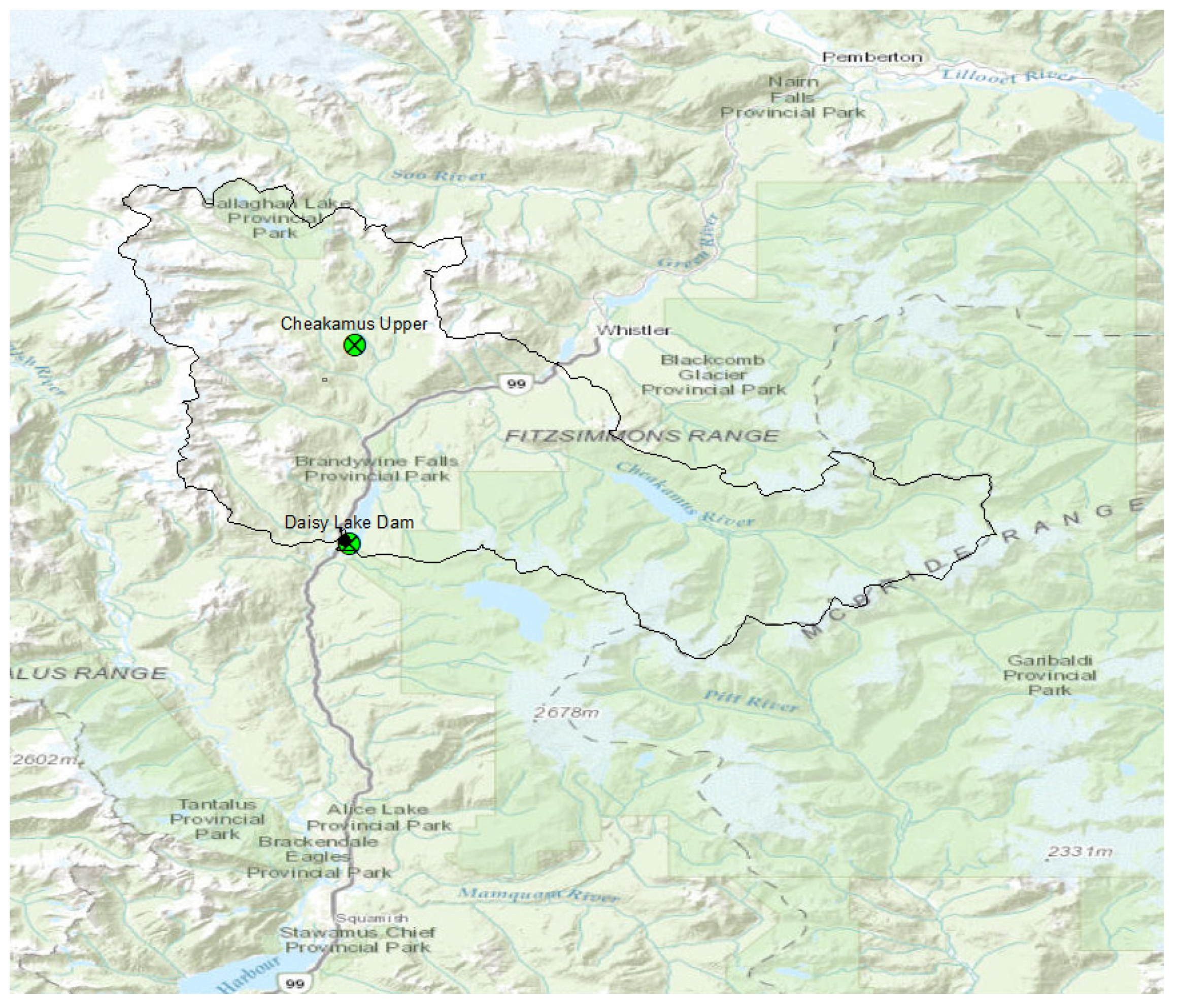
The Cheakamus River originates in the Fitzsimmons Range at Garibaldi Provincial Park, which is located about 25 km southeast of Whistler, BC. From its headwaters, the river flows through Cheakamus Lake and travels northwest towards Whistler, then turns south for approximately 46 km into Daisy Lake. Downstream of Daisy Lake, the Cheakamus River flows about 26 km to its confluence with the Squamish River, which in turn flows into Howe Sound. Elevations within the basin range from about 30 m above sea level at the confluence with the Squamish River (and 378 m at the dam), to 2625 m at Mount Overlord. The basin limits are defined by mountain peaks and glaciers, except at the valley bottom. Glaciers do not make up a large proportion of the basin area. The general trend of the river valley moving upstream from the Squamish River is north to north-easterly, and the river splits into two contributing sub-basins, flowing in from the southeast (Cheakamus) and northwest (Callaghan). The total basin area is about 1070 km2, with approximately 770 km2 upstream of the Cheakamus Dam [26]. The watershed boundary upstream of Cheakamus Dam is shown in Figure 3.
The climate in the Cheakamus Basin is transitional between the milder Pacific Coast and colder interior climatic regimes. Because of the orientation of the valley, winter southwesterly winds tend to transport moist air up Howe Sound and into the valley. There are three variations of Pacific Coast climate present within Cheakamus Basin. The most dominant one results from the confrontation of Pacific air masses with windward mountain slopes along the coast—resulting in prolonged and occasionally heavy rainfall on the westward slopes of the mountains. The second climatic variant is on the eastern (leeward) faces of the mountains, which have a much less rainy climate since Pacific air streams are typically descending, which disperses clouds resulting in decreased rainfall. The third variant results from the rain shadow of the Olympic Mountains in Washington state (U.S.), and results in hot sunny summers and rain confined to cooler seasons. There are effectively two climatic seasons—the first one from late September through March where a series of Pacific disturbances lead to fall and winter storms; and a summer season, where a pressure ridge typically dominates off the coast, occasionally interrupted by frontal activity. About half of the annual precipitation falls between October and January, and snow accumulates rapidly in the fall at higher elevations. Local orographic controls lead to micro-climates and spatially varying precipitation patterns within the basin.
The average annual precipitation from 1960 through 2020 at Daisy Lake Dam was 1782 mm, and the mean daily temperatures range from −1 °C in January to 17 °C in July. At Cheakamus Upper climate station, the average annual precipitation from 1960–2020 was 2307 mm. The difference in annual precipitation between these two climate stations is indicative of the significant spatial variability in precipitation across the basin. In general, precipitation along the valley bottom tends to decrease with distance away from Howe Sound, and precipitation is higher in the upper-elevation areas of the basin compared to the valley bottom.
The flow regime of the Cheakamus River follows a cyclical seasonal pattern in which flows begin to rise in April as increasing temperatures cause the snowpack to begin to melt. Typical freshet peak occurs in June or July, with flows decreasing significantly in August and September. The highest daily flows typically occur from September through January, due to rain-on-snow events. These events are relatively common because the temperature during these months tends to vary around the freezing point. The runoff magnitude during these rain-on-snow events is governed by the amount of rainfall, the existing snowpack, and the temperature sequence. Summer storms, while infrequent, can also produce extreme flooding. Flows into Daisy Lake tend to decrease in January, following the onset of below-freezing temperatures.
The minimum, maximum and average daily inflows into Daisy Lake from 1984–2021 are shown in Table 1. The average recorded inflow to Daisy Lake for this time period is 50 m3 s−1, equivalent to an average annual inflow volume of 1570 Million m3.
3.2. Hydrometeorological Data Sources
A number of data sources were utilized in this study for the development of hydrologic modelling inputs. These are all publicly available and are described below. The data listed here were applied with the methodology described in Section 2.2 to derive the various inputs to estimate the Cheakamus Dam PMF.
There are two BC Hydro Data Collection Platforms (DCP) stations within the Cheakamus basin that are used in calibration and validation of the Raven hydrologic model, and also for deriving the temperature inputs for the PMF scenarios. The stations used for temperature and precipitation data are listed in Table 2 and shown in Figure 3. The quality-controlled data from these stations is available from the Pacific Climate Impacts Consortium (PCIC) data portal.
The precipitation and temperature data from the above two climate stations were used to develop a calibration of the Raven hydrologic model, with the UBC Watershed Model emulation. This modelling software is open source and available online. Temperature data from the Daisy Lake Dam station were used to generate monthly values for both average daily temperature sequences and hourly temperature modulation. Where screening test runs showed that critical snowmelt temperature sequences preceding the seasonally adjusted PMP were able to produce considerable PMF volumes, 15-day 100-year critical temperature sequences were also generated, as described in Section 2.2.2, using the Daisy Lake Dam climate station. This was found to be the case for March and April, and therefore 15-day critical temperature sequences ending 15 March, 1 April and 15 April were generated (the PMP is considered to be out-of-season for May and June).
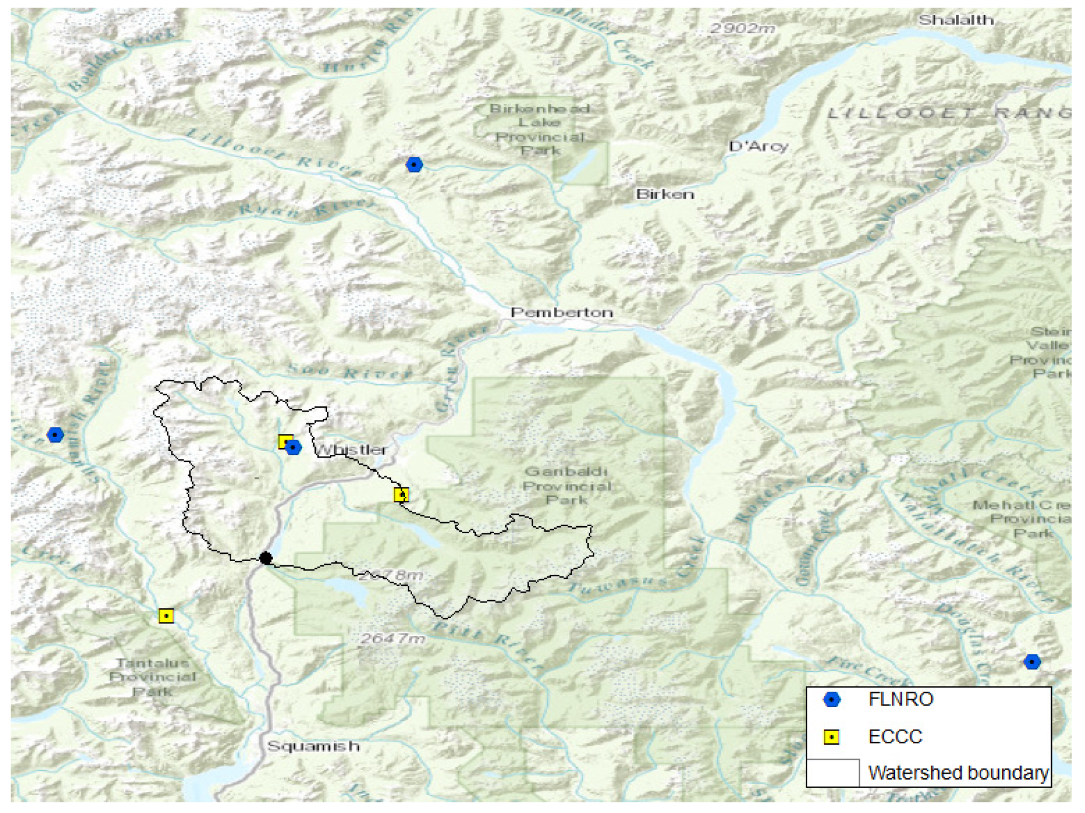
For the development of the 100-year snowpack, the following data sources were consulted, as shown in Table 3 and Figure 4. These stations have data available online at either Environment and Climate Change Canada (ECCC) or the BC Ministry of Forests, Lands and Natural Resources Operations (FLNRO) snow course data portal.
The ECCC stations generally provide continuous, automated snow-on-ground measurements. The FLNRO sources were a mix of automated daily data and monthly, manual snow-course measurements. The monthly manual measurements were taken a few days either before or after the first of each month from November through May or June. Since the majority of data sources had daily records, the monthly maximum values were taken from the records and analyzed in HYFRAN frequency analysis software to generate monthly maximum 100-year snowpacks for each station as described in Section 2.2.3. Stations with less than 10 years of records were omitted from the snow course data set.
Since the PMF simulations generally start on Day 1 of the month, it was assumed that the maximum results from October, November, January, February and March are approximately equal to the results on the first day of the following month, since snow is generally accumulating during the colder months of the year and is highest at the end of these months. In the later months, the monthly maximum was assumed to occur earlier in the month, and therefore the monthly maximum values from July are assumed to occur on the first of the month. This was considered to be a conservative way to use all of the available data instead of only first-of-month values.
The monthly maximum values were analyzed in HYFRAN software, and a number of distributions and fitting methods were tested to determine the best fit. Observed data were plotted over the fits with uncertainty bounds to visually determine the best fit to the datasets. The Gumbel distribution was generally well-fit to the data for all months and was typically the most conservative, and therefore it was used to develop relationships between elevation and 100-year snowpack as described in Section 2.2.3. The 100-year snowpack for each station is presented in Table 4.
3.3. Development of PMP
In the BC MetPortal, there are three transposition points near the Cheakamus Basin—28932, 1776 and 1827—that were considered for their potential to control the PMP. The PMS storms for the 1000 km2 area size at all durations and all three transposition points are based on a historical 144-h event that occurred on 8 January 2009 and has MetPortal storm ID 2009010830. The 24, 48, 72 and 96-h maximum Cheakamus Basin average precipitation amounts were calculated following the approach presented in Section 2.2.1. The basin areal average precipitation results for Cheakamus (area 720 km2) from the 48-h PMP events at each transposition point and corresponding to a 1000 km2 basin area are shown in Table 5. The 48-h duration was found to be governing for a 1000 km2 basin area—that is, the basin average values did not increase appreciably in the data for the 72-h or 96-h duration PMS events. It is clear from the table that there is significant scatter between transposition points in the basin average precipitation observed within the basin.
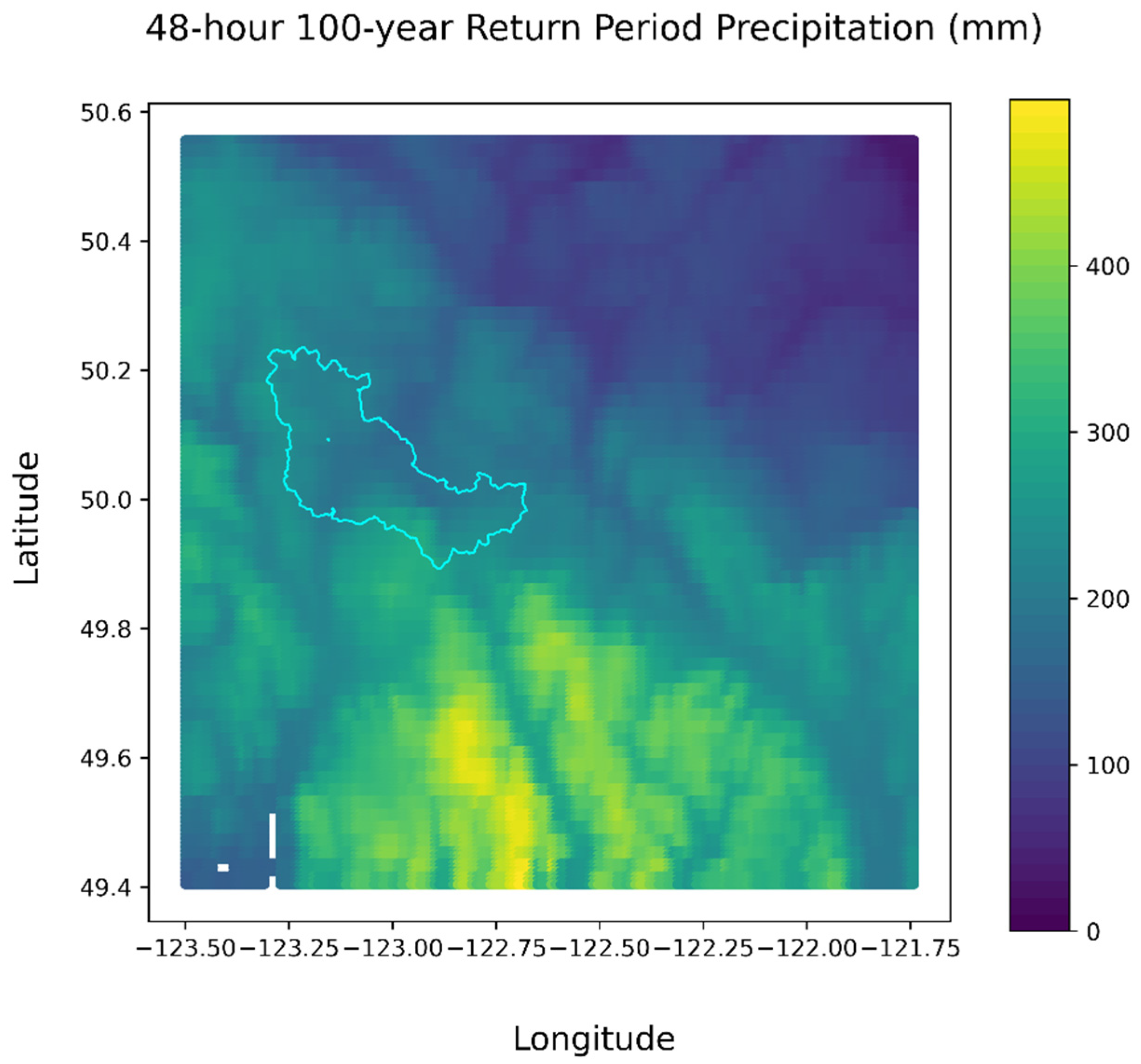
A plot of the transposition point locations with respect to the basin, along with the total storm raster data (sum of precipitation occurring at each location over 144 h) is shown in Figure 5. The values in Table 5 are visualized as precipitation footprints within Table 5. It is clear from the figure and table that the PMS from point 1827 (Figure 5b), although farthest from the dam, produces the most precipitation within the Cheakamus Dam watershed in comparison with the other readily available transposition points. This is a direct result of orographic influences. The apparent “eye” of the storm (the brightest yellow seen clearly for transposition points 28932 and 1776) is not able to be directly transposed over the transposition points or significantly further inland than it appears in the rasters. Since the transposition technique accounts for differences in the underlying topography, the area of highest storm precipitation is due to the orographic influence of the underlying mountainous topography, regardless of where the storm is transposed. Since the watershed terrain does not have as strong an influence on precipitation, the highest magnitudes within the storm occur over the mountains to the southeast of the watershed, rather than within the watershed itself. The storm centers are selected based on producing the greatest areal average that could occur over the watershed. This orographic influence can also be visualized in the 100-year return period precipitation, shown in Figure 6. It is important also to look at the precipitation footprint for the various transposition points. From each transposition point, there is a clear northwest-to-southeast trending precipitation footprint. None of the transposition points has effectively positioned this precipitation footprint over the Cheakamus Dam Basin, and therefore none of the three transposition points will provide the maximum possible precipitation within the basin itself. As such, a custom transposition was required and the results are presented in Figure 5d. The results from this custom transposition generated a 24-, 48- and 96-h maximum basin average precipitation of 238, 367 and 459 mm, respectively. There was about a 12% increase in the 48-h PMP from the highest readily available PMP estimate using Point 1827 (Figure 5b).
Using the PMS data from the custom transposition point, hydrologic modelling inputs were developed following the approach described in Section 2.2.1. For the Coastal South region, in which Cheakamus Dam is located, the all-season PMP (where 100% of the PMP could occur) is from October through February. PMP uncertainty was also analyzed for each of the macro-regions, and scaling factors are provided to assess what the 5th, median and 95th percentile precipitation values would be.
3.4. Development of 100-Year Pre-Storm
The 100-year pre-storm was generated using the 100-year point precipitation frequency raster for the 48-h period, shown in Figure 6. The basin average point precipitation frequency is calculated from the raster using the approach described in 2.2.1. An ARF is then applied, and the basin average precipitation is scaled into a realistic storm event with the same spatial and temporal characteristics of the PMS storm.
In order to determine an appropriate ARF for Cheakamus Basin, a number of sources were consulted. DTN has not provided official recommendations on ARF values in the BC MetPortal at this time, and the data for the storms analyzed and transposed into the basin are not readily accessible. However, some previous analysis results were available for guidance from a study at La Joie Dam, the Colorado–New Mexico regional extreme precipitation study [13], a 2003 BC regional PMP study, and original recommendations in HydroMeteorological Reports (HMR) [18,20,23]. The values presented in these studies for basin areas of 720 km2 are contrasted in Table 6 with values computed from the PMP storm provided through MetPortal. For the PMP storm ARF value, the 48-h total precipitation per grid cell within the basin was calculated and ranked, and the highest 25 km2 of grids were averaged and compared with the basin average 48-h PMP. It is important to note that the PMP is technically a maximized and transposed storm, from which an ARF would normally be calculated in-place and unmaximized. However, it provides a useful basin-specific comparison with the values derived in other studies.
From Table 6, it is clear that the ARF values from different sources and calculation methods vary significantly. The recommendations from HMR-57 and HMR-49 match quite closely. While these values are the most conservative, they also rely on older data and more dated methods (e.g., storm separation) to perform storm reconstructions and calculations. There is generally a fairly close agreement between the ARF calculated from the PMP for Cheakamus Basin (71%) and the recommended values from the recent Colorado–New Mexico study (72%), which included a storm-type-specific analysis of the mid-latitude cyclone (MLC)-type storms that create the most extreme precipitation events in the Cheakamus Basin. Discussion with DTN indicated this value would be a good proxy for Cheakamus since MLC events hitting western Colorado would have some similarities to Cheakamus.
Since the purpose of the pre-storm is to saturate the watershed, it is considered reasonably conservative to adopt the 72% ARF value for the 100-year basin average PMP, since this was calculated using the latest methods. Adopting a higher value will create more significant volume into the reservoir prior to the PMF, which may not be realistic, and would not significantly further saturate the watershed or lead to higher PMF flows.
The 48-h, 100-year precipitation basin average was calculated from the MetPortal point precipitation frequency raster data to be 237.7 mm. This was multiplied by an ARF of 72% for a 100-year storm basin average of 171.1 mm. This equates to about 46% of the PMP, which is in line with the generally accepted “rule of thumb” that the 100-year precipitation is less than or equal to 50% of the PMP. The ARF-adjusted value was scaled using the PMS storm, to give it a realistic spatial and temporal pattern and generate the HRU precipitation inputs for hydrologic modelling of the 100-year pre-storm.
3.5. Hydrological Modelling of PMF
To convert the PMP, snowpack and temperature inputs into flow estimates, rainfall-runoff modelling is required. As mentioned in Section 2.2, the Raven hydrological modelling framework [15] is used with the UBC Watershed Model emulation [16,17] to convert model forcings into estimates of the PMF. Both daily and hourly models were calibrated using point observations of precipitation and temperature from two gauges in the basin. The watershed was divided up based on elevation bands determined from a Digital Elevation Model, which were then further subdivided into Hydrological Response Units based on land cover and slope exposure. From the daily calibration, observed conditions at the onset of selected storm events were used as initial conditions in calibration of an hourly model. Severe storm events were selected from the fall/winter period, in addition to large rain-on-snow events from the spring freshet period to ensure snowmelt was adequately represented within the model.
To generate PMF inputs for the fall/winter events, inputs for each HRU consist of the 100-year pre-storm precipitation followed by two dry transition days, and then the PMP, which is followed by an additional dry period to allow simulation of the PMF recession. HRU temperatures during the pre-storm and PMP are derived by seasonally adjusting and elevation-lapsing the 1000 mb temperatures obtained from the MetPortal for the storm that produced the PMP. Temperatures during the dry periods correspond to average daily maximum temperatures, with average hourly diurnal temperature relationships applied for the month of interest. For snowmelt simulations, the 100-year pre-storm and its associated temperatures are replaced with 100-year critical snowmelt temperature sequences and average daily precipitation.
The PMF estimates are derived many times, first by varying the month to identify the critical PMF months, and then through sensitivity analysis that varies the watershed model parameters, temperatures, PMP magnitude, etc. to further explore the possible range of the estimates.
3.6. PMF Results and Discussion
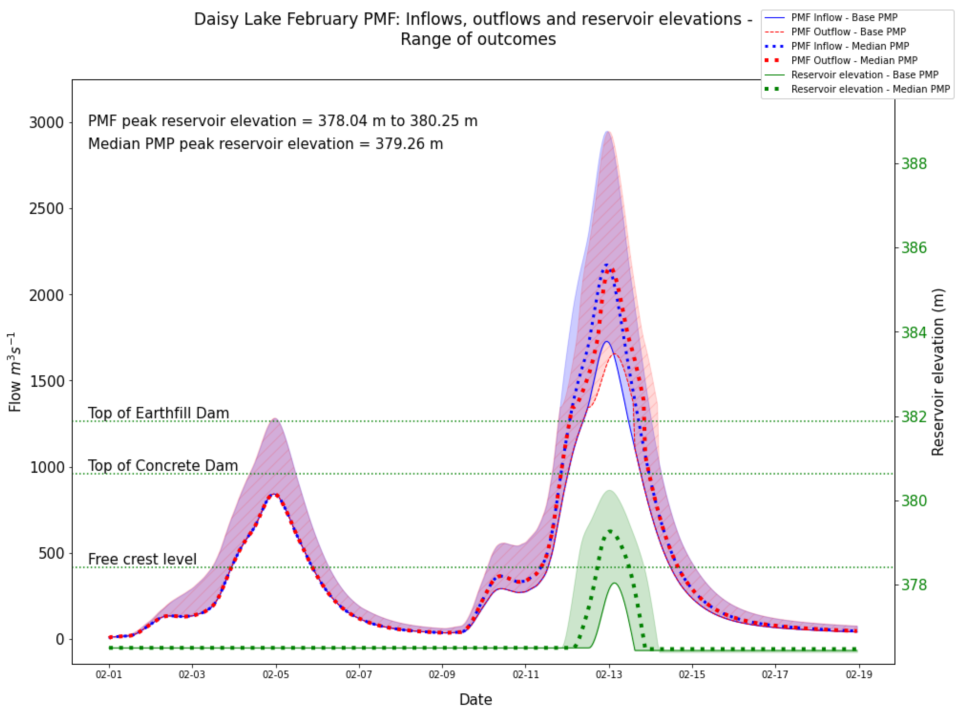
The governing PMF scenario for the Cheakamus Watershed was found to be the February scenario with a 100-year pre-storm, followed by two dry transition days and then the PMP. Snowmelt PMF scenarios were also computed and sensitivity analyses were performed on these. However, for this Coastal watershed, the winter rain-on-snow simulations produce the largest PMF estimates. A number of sensitivities were performed on the February base case scenario (the standard PMP directly from DTN)—including reducing the Fast Runoff Time Constant (FRTK) of the hydrologic model from 3 h down to 1 h as well as 20 min and the Interflow Runoff Time Constant (IRTK) from 3.5 days to 1 day. Snowmelt parameters were also varied to increase snowmelt runoff. The 95th percentile and median PMP scenarios were run, as well as an increased temperature scenario, where the climate change mean annual temperature change factors from [25] at Squamish and Whistler were spatially interpolated to the dam site and applied to the temperatures throughout the scenario. Finally, an extreme 95th percentile PMP scenario was run with increased temperatures applied, to represent the most extreme PMP. A check showed that the theoretical Clausius–Clapeyron relation (~7% per °C) for moderate climate change scenarios was well within the uncertainty bounds of the PMP. The scenario and sensitivities were routed through the Cheakamus Dam, assuming gates opened as required to keep the reservoir elevation at the seasonal Normal Maximum, until fully opened. The results from the February PMF simulations and all sensitivities are shown in Figure 7.
In the Figure 7, the results from the base-case PMP are shown as solid lines, and the results from the PMF sensitivity run based on the median PMP are shown as thicker dotted lines. Total sensitivity bounds are indicated by the shaded region. Blue lines and shading represent inflows, red represents outflows, and green represents the resultant reservoir elevations based on the PMF routing.
As can be seen from the figure, the February PMF has a median PMF peak one-hour inflow of 2171 m3 s−1 and a peak reservoir level of El. 379.26 m. The maximum uncertainty generated a peak one-hour inflow of 2949 m3 s−1 and a peak reservoir level of El. 380.25 m. The range of PMF estimates presented here represents significant reductions from the previously adopted PMF estimate for this specific facility (which was based on a PMP derived using the traditional approaches of the era). The decrease in the PMF estimate can be largely attributed to reduced precipitation totals from the PMP as derived using the newer storm transposition approach; the traditional storm separation approaches (similar to the methods described in HMR reports) tend to have more conservatism built in.
The February PMF is able to be routed through the facility without overtopping the concrete dam for all scenarios. Routing sensitivities are also recommended to assess facility performance should one or more discharge facilities be unavailable at the time of the flood.
4. Conclusions
This paper presents a methodology for the application of the BC MetPortal Probable Maximum Precipitation (PMP) and precipitation frequency estimates to evaluate the Probable Maximum Flood (PMF).
PMP and PMF estimates are being used for dam-safety assessments throughout the world. In many countries or jurisdictions dam owners are legally required to use the PMP/PMF concepts. This trend is likely to persist in the foreseeable future despite the fact that the PMP and PMF are deterministic concepts and cannot be used in quantitative dam-safety risk analyses. Historically, deriving PMP and corresponding PMF estimates has been done using different methods (site-specific or regional), data sources and by different analysts applying various levels of subjectivity and conservatism. This resulted in dam owners having a PMF estimate for a given dam changed (up or down) several times within the lifespan of a dam, leading to significant uncertainties in the dam owner’s ability to accurately assess the probability of dam failure and associated societal risks. The main benefit of the presented approach is the consistency in PMP estimates—the PMP estimate for each watershed in the province of British Columbia (area of 944,735 km2), regardless of its size, will be derived by the same analyst, the same storm database and will use the same methodology. Furthermore, this kind of large regional approach will improve the defensibility, increase the efficiency, and lower the cost of the completion of PMP/PMF studies in British Columbia. Another advantage is that the large amount of data are stored in the cloud and easily accessed by anyone through an online interface called MetPortal—the PMP package contains most of the hydrometeorological information a hydrologist requires for modelling extreme floods, without having to fabricate synthetic, potentially unrealistic storm events using old, out-of-date methods. The utilized ESTP approach strives to eliminate assumptions associated with traditional PMP determination technique and uses real storm patterns instead of synthetic, conservatively created storms, also known as “frankenstorms”. In other words, the methodology presented in this paper will be a welcome improvement for all dam owners, practitioners and regulators in jurisdictions where it is a legal requirement to develop PMP and PMF estimates for both the design of new dams and dam-safety assessments of existing/ageing dams.
In this paper, generic data processing flowcharts are presented that can be applied to evaluate the basin average PMP and generate hydrologic modelling inputs from the Probable Maximum Storm (PMS) data in the MetPortal, while preserving the spatial and temporal characteristics of the storm. The processing tools were developed using Python programming language, but the same general flow could be applied within GIS or other programming environments, depending on what the practitioner is comfortable with (the process flow could also be applicable in other regions where spatially and temporally intact PMP estimates are available). An approach is suggested to develop a 100-year frequency pre-storm to saturate the watershed using MetPortal point precipitation frequency estimates. Details on developing snowpack and temperature inputs for hydrologic modelling are also provided.
The approach is applied to the Cheakamus Basin north of Squamish, BC. A detailed description of how to assess transposition points for their potential to control the PMP in the basin is provided, as well as a description of 100-year pre-storm, temperature inputs, and snowpack for the basin. Results are presented with the uncertainty bounds included. It is important for practitioners to convey to dam owners that the PMF is an estimate that has uncertainty associated with it—part of which is assessed using sensitivity analysis. A single value estimate does not express this uncertainty and can be misleading.
In the future, other regions may wish to take advantage of this regional PMP approach applied in the BC MetPortal, to significantly improve the consistency of PMF estimates between watersheds. In British Columbia, the BC MetPortal would benefit from additional work to develop regional estimates of Areal Reduction Factors (ARFs) for watersheds greater than 25 km2. Future research directions pertaining to evaluation of the PMF could consider application of Monte Carlo uncertainty analysis, similar to the approach used for the PMP, which would improve the estimation of the possible range of PMF estimates and their likelihood.
Author Contributions
Conceptualization, L.M.K. and Z.M.; methodology, L.M.K. and Z.M.; software, L.M.K.; validation, L.M.K.; formal analysis, L.M.K.; investigation, L.M.K.; data curation, L.M.K.; writing—original draft preparation, L.M.K.; writing—review and editing, Z.M.; visualization, L.M.K.; supervision, Z.M.; project administration, L.M.K.; funding acquisition, Z.M. All authors have read and agreed to the published version of the manuscript.
Funding
This research was funded by BC Hydro.
Institutional Review Board Statement
Not applicable.
Informed Consent Statement
Not applicable.
Data Availability Statement
Data utilized in this study are available from the following sources: PMP and Point Precipitation Frequency estimates available from BC MetPortal at https://dtn-metportal.shinyapps.io/bc_region/ (accessed on 15 May 2021); Hydrometeorological data available from ECCC at https://climate.weather.gc.ca/historical_data/search_historic_data_e.html (accessed on 30 July 2021), FLNRO at https://www2.gov.bc.ca/gov/content/environment/air-land-water/water/water-science-data/water-data-tools/snow-survey-data (accessed on 30 July 2021), and PCIC data portal at https://data.pacificclimate.org/portal/pcds/map/ (accessed on 30 July 2021). Due to BC Hydro’s confidentiality policy, the calibrated watershed model, rating curves for reservoir routing and python script for development of PMF inputs are not provided.
Acknowledgments
The authors would like to acknowledge BC Hydro for funding this study. Thanks also to Jennifer Finkenbine of BC Hydro, who has carefully checked and reviewed this work for accuracy. Additional thanks to Tye Parzybok, Katie Ward, Debbie Martin and Lauren Elston of DTN for providing support and advice throughout the project.
Conflicts of Interest
The authors declare no conflict of interest.
References
- Canadian Dam Association. Dam Safety Guidelines; CDA: Markahm, ON, Canada, 2013. [Google Scholar]
- International Commission on Large Dams. Flood Evaluation and Dam Safety, 1st ed.; CRC Press: Boca Raton, FL, USA, 2018. [Google Scholar]
- Chen, X.; Hossain, F. Understanding future safety of DAMs in a changing climate. Bull. Am. Meteorol. Soc. 2019, 100, 1395–1404. [Google Scholar] [CrossRef]
- Micovic, Z.; Hartford, D.N.D.; Schaefer, M.G.; Barker, B.L. A non-traditional approach to the analysis of flood hazard for dams. Stoch. Environ. Res. Risk Assess. 2016, 30, 559–581. [Google Scholar] [CrossRef]
- International Commission on Large Dams. ICOLD European Club—Dam Legislation; ICOLD: Paris, France, 2020. [Google Scholar]
- World Meteorological Organization. Manual on Estimation of Probable Maximum Precipitation; WMO: Geneva, Switzerland, 2009. [Google Scholar]
- Micovic, Z.; Schaefer, M.G.; Taylor, G.H. Uncertainty analysis for Probable Maximum Precipitation Estimates. J. Hydrol. 2015, 521, 360–373. [Google Scholar] [CrossRef]
- World Meteorological Organization. Manual for Depth-Area-Duration Analysis of Storm Precipitation (WMO-237); WMO: Geneva, Switzerland, 1969. [Google Scholar]
- DTN; MGS Engineering. British Columbia Extreme Flood Project, MetPortal User’s Guide—Probable Maximum Precipitation and Precipitation-Frequency Analysis for British Columbia (Bulletin 2020-5-PMP/RFPA); MetStat: Fort Collins, CO, USA, 2020. [Google Scholar]
- Ward, K.L.; Sankovich-Bahls, V.; Hendricks-Dietrich, A.; Parzybok, T.W.; McLean, R.; Micovic, Z.; Duren, A.M. A novel approach for developing regional Probable Maximum Precipitation guidelines. In Proceedings of the USSD 2020 Annual Conference, Denver, CO, USA, 20–24 April 2020. [Google Scholar]
- DTN; MGS Engineering. British Columbia Extreme Flood Project, Probable Maximum Precipitation Guidelines for British Columbia—Technical Report (Bulletin 2020-3-PMP); MetStat: Fort Collins, CO, USA, 2020. [Google Scholar]
- DTN MetPortal—One-Stop Access to Online Precipitation-Frequency Tools and Data. Available online: https://www.dtn.com/weather/utilities-and-renewable-energy/metportal/ (accessed on 5 December 2021).
- Schaefer, M.G.; Taylor, G.H.; Parzybok, T.W. Regional Precipitation-Frequency Analysis Using the Climate Region Method for Application in Analyses of Extreme Precipitation and Floods; Colorado Division of Water Resources: Denver, CO, USA, 2018. [Google Scholar]
- World Meteorological Organization. Estimation of Maximum Floods (Technical Note No. 98); WMO: Geneva, Switzerland, 1969. [Google Scholar]
- Craig, J.R.; Brown, G.; Chlumsky, R.; Jenkinson, R.W.; Jost, G.; Lee, K.; Mai, J.; Serrer, M.; Sgro, N.; Shafii, M.; et al. Flexible watershed simulation with the Raven hydrological modelling framework. Environ. Model. Softw. 2020, 129, 104728. [Google Scholar] [CrossRef]
- Quick, M.C.; Pipes, A.U.B.C. Watershed Model. Hydrol. Sci. J. 1977, 22, 153–161. [Google Scholar] [CrossRef]
- Micovic, Z.; Quick, M.C. A rainfall and snowmelt runoff modelling approach to flow estimation at ungauged sites in British Columbia. J. Hydrol. 1999, 226, 101–120. [Google Scholar] [CrossRef]
- Reichelderfer, F.W. Rainfall Intensity-Frequency Regime Part 2-Southeastern United States. (HMR-29); National Weather Service: Washington, DC, USA, 1958. [Google Scholar]
- Hershfield, D.M. Rainfall Frequency Atlas of the United States, for Durations from 30 Minutes to 24 Hours and Return Periods from 1 to 100 Years (HMR No. 40); National Weather Service: Washington, DC, USA, 1961. [Google Scholar]
- Miller, J.F. Two-to-Ten-Day Precipitation for Return Periods of 2 to 100 Years in the Contiguous United States (HMR No. 49); National Weather Service: Washington, DC, USA, 1964. [Google Scholar]
- Kao, S.-C.; DeNeale, S.T.; Yegorova, E.; Kanney, J.; Carr, M.L. Variability of precipitation areal reduction factors in the conterminous United States. J. Hydrol. 2020, 9, 100064. [Google Scholar] [CrossRef]
- Pavlovic, S.; Perica, S.; St Laurent, M.; Mejia, A. Intercomparison of selected fixed-area areal reduction factor methods. J. Hydrol. 2016, 537, 419–430. [Google Scholar] [CrossRef]
- Hansen, E.M.; Fenn, D.; Corrigan, P.; Vogel, J. Probable Maximum Precipitation—Pacific Northwest States Columbia River (including Portions of Canada), Snake River and Pacific Coastal Drainages (HMR No. 57); National Weather Service: Washington, DC, USA, 1994. [Google Scholar]
- The World Bank. Good Practice Note on Dam Safety—Technical Note 1—Hydrological Risk; The World Bank: Washington, DC, USA, 2021. [Google Scholar]
- Cannon, A.J.; Jeong, D.I.; Zhang, X.; Zwiers, F.W. Resilient Buildings and Core Public Infrastructure: An Assessment of the Impact of Climate Change on Climatic Design Data in Canada; Environment and Climate Change Canada: Gatineau, QC, Canada, 2020. [Google Scholar]
- BC Hydro. Cheakamus Project Water Use Plan; BC Hydro: Vancouver, BC, Canada, 2005. [Google Scholar]
Figure 1.
Flow chart showing Python program flow for computation of basin average precipitation during Probable Maximum Storm.
Figure 1.
Flow chart showing Python program flow for computation of basin average precipitation during Probable Maximum Storm.

Figure 2.
Flow chart showing Python program flow for generation of hydrological modelling Hydrological Response Unit (HRU) inputs.
Figure 2.
Flow chart showing Python program flow for generation of hydrological modelling Hydrological Response Unit (HRU) inputs.

Figure 3.
Location of British Columbia (BC) Hydro climate stations within the Cheakamus Basin.

Figure 4.
Location of snow course data in the vicinity of Cheakamus Basin.

Figure 5.
Cheakamus Basin— Probable Maximum Storm (PMS) total storm raster data from three nearby transposition points, shown in red (a) 1776, (b) 1827, and (c) 28932, as well as (d) from a custom storm transposition, with the custom transposition point shown with a white x.
Figure 5.
Cheakamus Basin— Probable Maximum Storm (PMS) total storm raster data from three nearby transposition points, shown in red (a) 1776, (b) 1827, and (c) 28932, as well as (d) from a custom storm transposition, with the custom transposition point shown with a white x.

Figure 6.
Cheakamus Basin and surrounding area—100-year return period point precipitation frequencies.
Figure 6.
Cheakamus Basin and surrounding area—100-year return period point precipitation frequencies.

Figure 7.
Cheakamus Basin February PMP and uncertainty bounds, with inflows, outflows and reservoir elevations shown.
Figure 7.
Cheakamus Basin February PMP and uncertainty bounds, with inflows, outflows and reservoir elevations shown.


Table 1.
Daisy Lake inflow statistics, 1984–2021.
| Month | Average Daily Inflow m3 s−1 | Minimum Daily Inflow m3 s−1 | Maximum Daily Inflow m3 s−1 |
|---|---|---|---|
| January | 25 | 3.6 | 371 |
| February | 21 | <1 | 321 |
| March | 23 | 1.0 | 218 |
| April | 37 | 6.4 | 186 |
| May | 79 | 14.1 | 251 |
| June | 105 | 44.5 | 298 |
| July | 95 | 35.1 | 293 |
| August | 61 | <1 | 623 |
| September | 38 | 10.4 | 217 |
| October | 41 | 2.1 | 627 |
| November | 45 | <1 | 648 |
| December | 25 | 3.4 | 355 |
Table 2.
BC Hydro data collection platforms in Cheakamus Watershed.
| Station Name | Station Code | Record Period | Elevation | Latitude | Longitude |
|---|---|---|---|---|---|
| Daisy Lake Dam | 21211 | 1960–2021 | 390 m | 49.975 | −123.137 |
| Cheakamus Upper | 21123 | 1960–2021 | 880 m | 50.116 | −123.133 |
Table 3.
BC Hydro data collection platforms in Cheakamus Watershed.
| Station Name | Station Code | Source | Record Period | Elevation | Latitude | Longitude |
|---|---|---|---|---|---|---|
| Callaghan Valley | 1101300 | ECCC | 2005–2021 | 884 m | 50.144 | −123.111 |
| Whistler Roundhouse | 1108906 | ECCC | 1980–2021 | 1835 m | 50.068 | −122.947 |
| Squamish Upper | 1047672 | ECCC | 1980–2010 | 46 m | 49.896 | −123.281 |
| Squamish River Upper | 3A25P | FLNRO | 1989–2021 | 1340 m | 50.153 | −123.441 |
| Callaghan Creek | 3A20P | FLNRO | 1976–2021 | 1040 m | 50.136 | −123.102 |
| Tenquille Lake | 1D06 | FLNRO | 2000–2021 | 1680 m | 50.536 | −122.930 |
| Nahatlatch Creek | 1D10 | FLNRO | 1968–2021 | 1550 m | 49.830 | −122.051 |
Table 4.
100-year snowpack estimates at various climate stations.
| Station | El (m) | 100-Year Snowpack (cm) | ||||||
|---|---|---|---|---|---|---|---|---|
| October | November | December | January | February | March | April | ||
| Squamish Upper | 46 | 0 | 49 | 120 | 155 | 163 | 116 | 56 |
| Callaghan Valley | 884 | - | 184 | 267 | 311 | 366 | 397 | 356 |
| Callaghan Creek | 1040 | - | - | 254 | 349 | 413 | 442 | 385 |
| Squamish River Upper | 1340 | - | 81 | 133 | 190 | 247 | 286 | 291 |
| Nahatlatch | 1550 | - | - | 134 | 170 | 192 | 260 | 287 |
| Tenquille | 1680 | 21 | 57 | 91 | 114 | 149 | 182 | 255 |
| Whistler Roundhouse | 1835 | 69 | 259 | 337 | 404 | 440 | 485 | 470 |
Table 5.
Basin average precipitation from the 48-h Probable Maximum Precipitation (PMP) at transposition points near Cheakamus Basin.
Table 5.
Basin average precipitation from the 48-h Probable Maximum Precipitation (PMP) at transposition points near Cheakamus Basin.
| Transposition Point | Cheakamus Basin Average Precipitation, from 48-h PMP | ||
|---|---|---|---|
| 24-h Max | 48-h Max | 96-h Max | |
| 28932 | 202 | 316 | 394 |
| 1776 | 142 | 228 | 289 |
| 1827 | 213 | 323 | 406 |
Table 6.
Comparison of Areal Reduction Factors from various sources.
| Source | Location | ARF for 720 km2 Basin Area |
|---|---|---|
| Computed from Cheakamus watershed transposed PMS | Transposed to Cheakamus Basin | 71% |
| HMR-49 [20] | Contiguous United States | 93.5% |
| HMR-57 [23] | Pacific Coastal Drainage | 89% |
| Confidential Study | Southwestern British Columbia | 93.5% |
| Confidential Study | La Joie Basin | 59% |
| Colorado-New Mexico extreme precipitation study [13] | Western macro-climate region of Colorado-New Mexico | 72% |
Publisher’s Note: MDPI stays neutral with regard to jurisdictional claims in published maps and institutional affiliations. |
© 2022 by the authors. Licensee MDPI, Basel, Switzerland. This article is an open access article distributed under the terms and conditions of the Creative Commons Attribution (CC BY) license (https://creativecommons.org/licenses/by/4.0/).
Share and Cite
MDPI and ACS Style
King, L.M.; Micovic, Z. Application of the British Columbia MetPortal for Estimation of Probable Maximum Precipitation and Probable Maximum Flood for a Coastal Watershed. Water 2022, 14, 785. https://doi.org/10.3390/w14050785
AMA Style
King LM, Micovic Z. Application of the British Columbia MetPortal for Estimation of Probable Maximum Precipitation and Probable Maximum Flood for a Coastal Watershed. Water. 2022; 14(5):785. https://doi.org/10.3390/w14050785
Chicago/Turabian StyleKing, Leanna M., and Zoran Micovic. 2022. "Application of the British Columbia MetPortal for Estimation of Probable Maximum Precipitation and Probable Maximum Flood for a Coastal Watershed" Water 14, no. 5: 785. https://doi.org/10.3390/w14050785
Note that from the first issue of 2016, this journal uses article numbers instead of page numbers. See further details here.