Numerical Experiment on Salt Transport Mechanism of Salt Intrusion in Estuarine Area

Abstract

The process of exchange and transport between salt and fresh water is affected by not only convection due to the density gradient but also turbulence. In this study, a high resolution mathematical model of the intrusion movement of saltwater in an estuary area was established and compared with a physical flume experiment. The model, whose minimum horizontal grid cell of the model is 0.05 m, and minimum vertical grid cell is 0.0005 m, simulated well the salt transport mechanism at the interface between salt and fresh water. The salt transport processes of estuarine saltwater intrusion were obtained under the conditions of no runoff and no tide, no runoff and tide, and runoff and tide. The results suggest that under the joint action of runoff and tide, the mixing process in the interface of salt and fresh water is relatively gentle, the change in the velocity gradient is small, and the advance distance of saltwater intrusion will reach a dynamic equilibrium state after a period of time.

1. Introduction

In estuaries, under the action of dynamic factors such as river runoff and tide, fresh water moves seaward in the upper layer due to its relatively low density, while salty seawater moves landward in the lower layer due to its higher density. Stratification and mixing are a result of this interaction.

To thoroughly understand the engineering problems associated with this process and formulate numerical simulation results that accurately fit the reality, numerical investigation on saltwater intrusion has gradually developed from two-dimensional (2D) to three-dimensional (3D), which can analyze the change rules of many dynamic factors in all directions. At present, the prevailing 3D models for estuarine numerical simulation include the EFDC model of the United States Environmental Protection Agency, the FVCOM model of the University of Massachusetts, the POM Model of Princeton University, the ECOM model, the ECOMSED model, the ROMS model and so on. Many previous numerical simulations of saltwater intrusion were carried out by the ocean models above. Krvavica et al. [1] used numerical simulations to study the impact of sea level rise on salinity intrusion in estuaries based on three indicators: salt wedge intrusion length, sea water volume, and river inflow required to restore saltwater intrusion. Zhang et al. [2] established a 3D numerical model based on the SEAWAT program to simulate the saline intrusion of the coastal aquifer of the Dagu River Basin near Jiaozhou Bay. This was conducted to explore the impact of increasing groundwater recharge and decreasing groundwater extraction on reducing water pollution in the future. For large-scale models, there is much research at present, and it is relatively perfect. However, the number of studies on the application of small and medium scale models is still relatively small. Hu [3] and Liu [4,5] simulated and analyzed the saltwater intrusion in the Modaomen waterway based on the EFDC model and FVCOM model, respectively, but as a large-scale model, it can only reflect the salinity change in a large area. In the study of saltwater intrusion, the existing research results mostly used the above ocean models. In this study, instead of those models, computational fluid dynamics models based on Navier–Stokes equations were used to study the hydrodynamic characteristics of saltwater intrusion. By adding the saltwater and freshwater exchange module into the computational fluid dynamics model, the numerical model was established. The simulation results were then compared with the existing measured data to verify the model’s fitting degree.

During saltwater intrusion, the various hydrodynamic characteristics of the interface between salt and fresh water are more complex. The process is influenced by many factors. To get accurate results, the size of vertical stratification of the simulation domain needs to be smaller. Cheng [6], Zheng [7], and Lyu [8] used different ocean models to simulate the estuarine areas in different regions by vertical stratification, with a minimum of only 6 layers and a maximum of 20 layers. In the ocean models that they used, the 3D baroclinic original equation is mostly used to simulate. Although vertical stratification is also applied, generally only meso-scale simulation can be carried out, which cannot be finer. Although the hydrodynamic characteristics of different water layers can be simulated more finely by vertical stratification, models with high grid resolution and many layers cause a high computational demand. Hence, vertical stratification with a great amount of layers can hardly be achieved. Therefore, the numerical simulation of saltwater intrusion needs to be developed in the direction of small-scale refinement—that is, the application of an increasing number of fine high-resolution grid cells or hybrid grid cells. To thoroughly study the hydrodynamic changes at the interface between salt and fresh water of the saltwater intrusion movement, it is necessary to reduce the vertical scale to realize the small-scale fine numerical simulations of the saltwater intrusion movement. Furthermore, it may also be beneficial to go even smaller than the stratification spacing scale used in traditional oceanographic observations. Bao and Ren [9] used the minimum resolutions of 0.5 m and 3 m vertically to reflect the salinity change process of saltwater intrusion in rising and falling tides in the Lingdingyang Estuary through a 3D baroclinic model, but this fineness still cannot reflect the salinity change rate in each layer. Kim et al. [10] applied the continuity and Navier–Stokes equations as the governing equations for incompressible fluid motion, and a numerical wavemaker was employed to reproduce offshore wave environment. Grid convergence test against grids number was carried out to investigate grid dependency. The error between the calculation results obtained by the high-resolution grids and the measured values was smaller. In this study, the continuity and NS equations were also used as the governing equations, and the mixing interface layer of salt and fresh water, small circulation, and eddy currents all occurred in a small vertical domain ranging from 0.05 m to 0.1 m. Increasing the vertical grid resolution can effectively resolve the numerical dispersion problem and improve the calculation accuracy. The relative water depth of the minimum vertical grid cell was 0.001667, and the time step was set to 0.0005 s, which can simulate well the process of the mixing interface layer of salt and fresh water, small circulation, and eddy currents.

To represent the hydrodynamic characteristics of the interface between salt and fresh water caused by saltwater intrusion, the density difference was considered, and then the vertical resolution of the model was refined. To reduce the computational demand, the vertical stratification of the overlying water body was appropriately reduced in the area where there was no apparent salinity change. In this study, the Navier–Stokes equation was directly solved to simulate the movement of saltwater intrusion. The results were compared with existing experimental data of a physical tank model of saltwater intrusion to analyze the movement mechanism and hydrodynamic characteristics of saltwater intrusion.

This model has the following assumptions: Reynolds-averaged turbulent model, incompressible fluid, no temperature-variation, and exclusions of wind and wave. Due to the use of high-resolution grids, the limitation of calculation demand and calculation speed will also affect the research. Although with the acknowledgment of those limitations above, wind, wave, temperature, sediment, and other factors can be added to the study in future work. Specifically, it can be used to study the salinity change in estuary at a small scale, the interface of the mixing of salt and fresh water, and the convection and diffusion of salt between water and sediment.

2. Mathematical Model of Saline Water Intrusion and Verification Data

2.1. Control Equation of the Mathematical Model

The mathematical model of the saltwater intrusion movement under baroclinic pressure, considering the change in density, is composed of the following equations [11]:

(1)

the continuity equation:

$$\frac{\partial \left(\varphi \rho \right)}{\partial t}+\frac{\partial }{\partial x_i}\left(\varphi \rho u_i\right)=0$$

(1)

(2)

the momentum equation:

$$\frac{\partial \left(\varphi \rho u_i\right)}{\partial t}+\frac{\partial }{\partial x_j}\left(\varphi \rho u_i{u}_j\right)=-\frac{\partial \left(\varphi \rho \right)}{\partial x_j}+\frac{\partial }{\partial x_j}\left(\varphi \mu \frac{\partial u_i}{\partial u_j}-\varphi \rho \overline{{u^{\prime }}_i{u^{\prime }}_j}\right)+S_{M,i}$$

(2)

(3)

the salt transport equation:

$$\frac{\partial \left(\varphi \rho S\right)}{\partial t}+\frac{\partial }{\partial x_j}\left(\varphi \rho u_{j}S\right)=\varphi \left(\rho \lambda +\frac{{\mu }_t}{S{c}_t}\right)\frac{\partial }{\partial x_j}\left(\frac{\partial S}{\partial x_j}\right)+S_{S,j}$$

(3)

(4)

the state equation:

$$\begin{array}{cc}\hfill \rho \left(T,S\right)& =a_1+a_{2}T+a_3{T}^2+a_4{T}^3+a_5{T}^4+a_6{T}^5\hfill \\ & +S\left(a_7+a_{8}T+a_9{T}^2+a_{10}{T}^3+a_{11}{T}^4\right)\hfill \\ & +S^{2/3}\left(a_{12}+a_{13}T+a_{14}{T}^2\right)+a_{15}{S}^2\hfill \end{array}$$

(4)

where $i$, $j$ can be taken as 1, 2, and 3 respectively; $u_i$ is the velocity in the x, y, and z directions; $x_i$ is x, y, and z directions; $\varphi$ is the porosity; $\rho$ is a function of density with respect to temperature and salinity; $-\rho \overline{u_i^{\prime }{u}_j^{\prime }}$ is the Reynolds stress; $t$ is the time; $\mu$ is the dynamic viscosity coefficient; $S_{M,i}$ is the resistance source term of the momentum equation in the x, y, and z directions; $S_{S,j}$ is the source term of the salt transport equation in the x, y, and z directions; $S$ is the salinity; ${\mu }_t$ is the turbulent viscosity; $S_{C_t}$ is the turbulent Schmidt number, value = 0.7; $\lambda$ is the molecular diffusion coefficient; $T$ is the sea water temperature, taking the fixed value; and, $a_1~a_{15}$ is the empirical coefficient.

2.2. Physical Tank Experiment

Zhang et al. [12] simulated the saltwater intrusion in the Modaomen waterway of the Pearl River Estuary using a physical flume experiment. Based on that experiment, this study established and verified a numerical model of salt tide intrusion.

Figure 1 shows the top view of technical sketch of the above-mentioned physical model tank, which is composed of a twisted water channel, straight glass tank, and tide-generating system. The vitreous tank is 110 m long, 0.5 m wide, and 0.5 m high. To make the physical model resemble the Modaomen waterway as much as possible, the twisted waterway part was designed in that way, as shown in the left part of the Figure 1, as twisting can play a part in the function of the receiving tide. The front end of the twisted channel of the physical tank controls the runoff by the flowmeter, and the downstream tidal system can control the change in water level.

3. Numerical Simulation and Verification of the Saltwater Intrusion Movement

3.1. No-Runoff and No-Tide Condition

3.1.1. Model Set-Up of the No-Runoff and No-Tide Condition

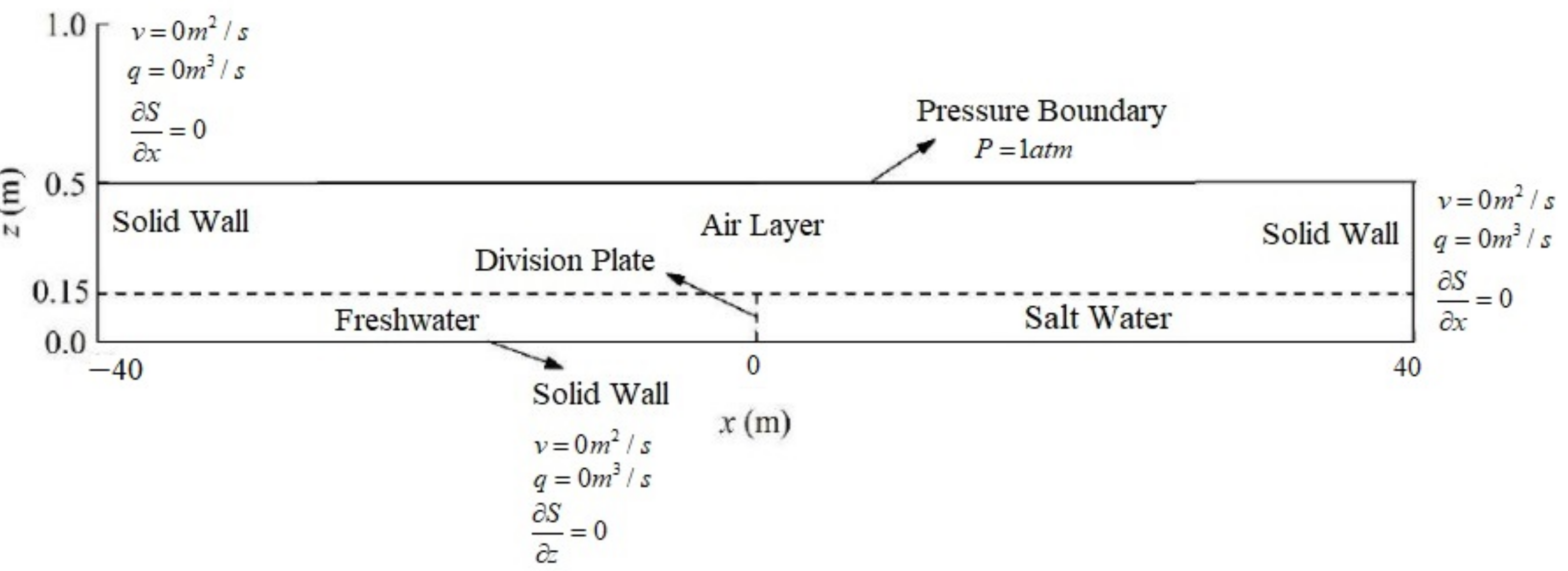
The numerical model under the no-runoff and no-tide condition is shown in Figure 2. The entire model was 80 m long, and the initial water depth was 0.15 m. A division plate was placed in the middle. The left side of the division plate was the freshwater area, right side was the saltwater area, and salinity (S) was 10.5‰. Since there were no other external force factors, and the initial velocity was 0 m/s, except for the upper boundary that was the pressure boundary of standard atmospheric pressure, the other boundaries adopted solid wall boundary conditions.

The main reason for simulating the upstream saltwater process without runoff and tide is to verify whether the numerical model can accurately reflect the movement process under the action of only the salinity gradient. Without the influence of external dynamic factors, the interface between the salt and fresh water was wedge-shaped. To better reflect the mixing movement of salt and fresh water at the interface, it was divided into 1600 grid cells horizontally and 500 grid cells vertically. The Courant number in the model was set to 0.5.

3.1.2. Velocity Distribution

Two empirical equations for the front-end velocity of the stratified density flow were proposed by Benjamin [13] and Turner [14], as seen in Equations (5) and (6):

$$U_{Head,B}=0.5\sqrt{\frac{g}{{\rho }_2}\left({\rho }_2-{\rho }_1\right)h}$$

(5)

$$U_{Head,T}=0.47\sqrt{\frac{g}{{\rho }_2}\left({\rho }_2-{\rho }_1\right)h}$$

(6)

where Equation (6) considers the flow viscosity effect, and h is the water depth of the flume. The velocity of the front end of the saltwater intrusion obtained by the two equations was $U_{Head,B}$ = 0.054 m/s and $U_{Head,T}$ = 0.051 m/s.

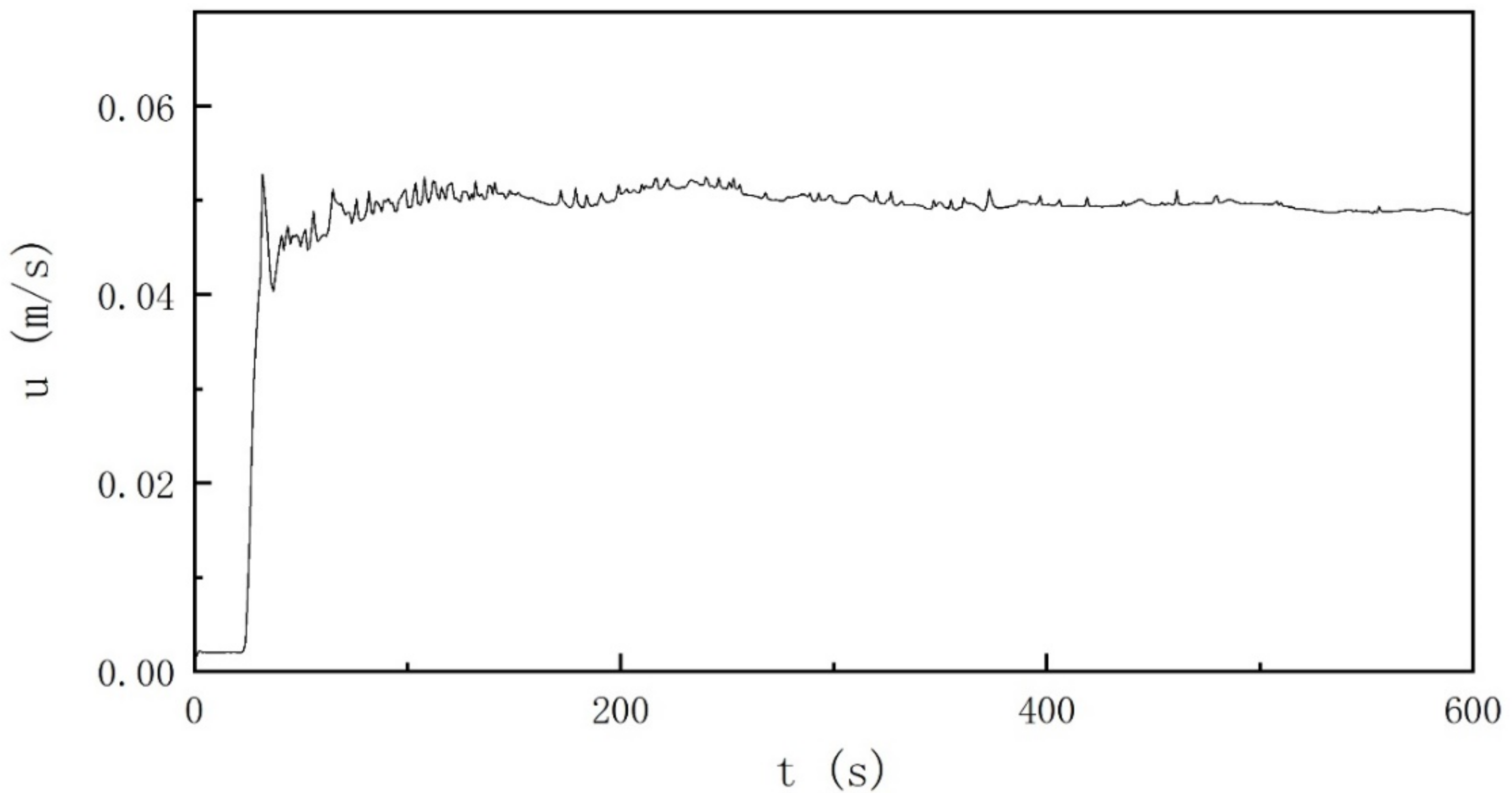
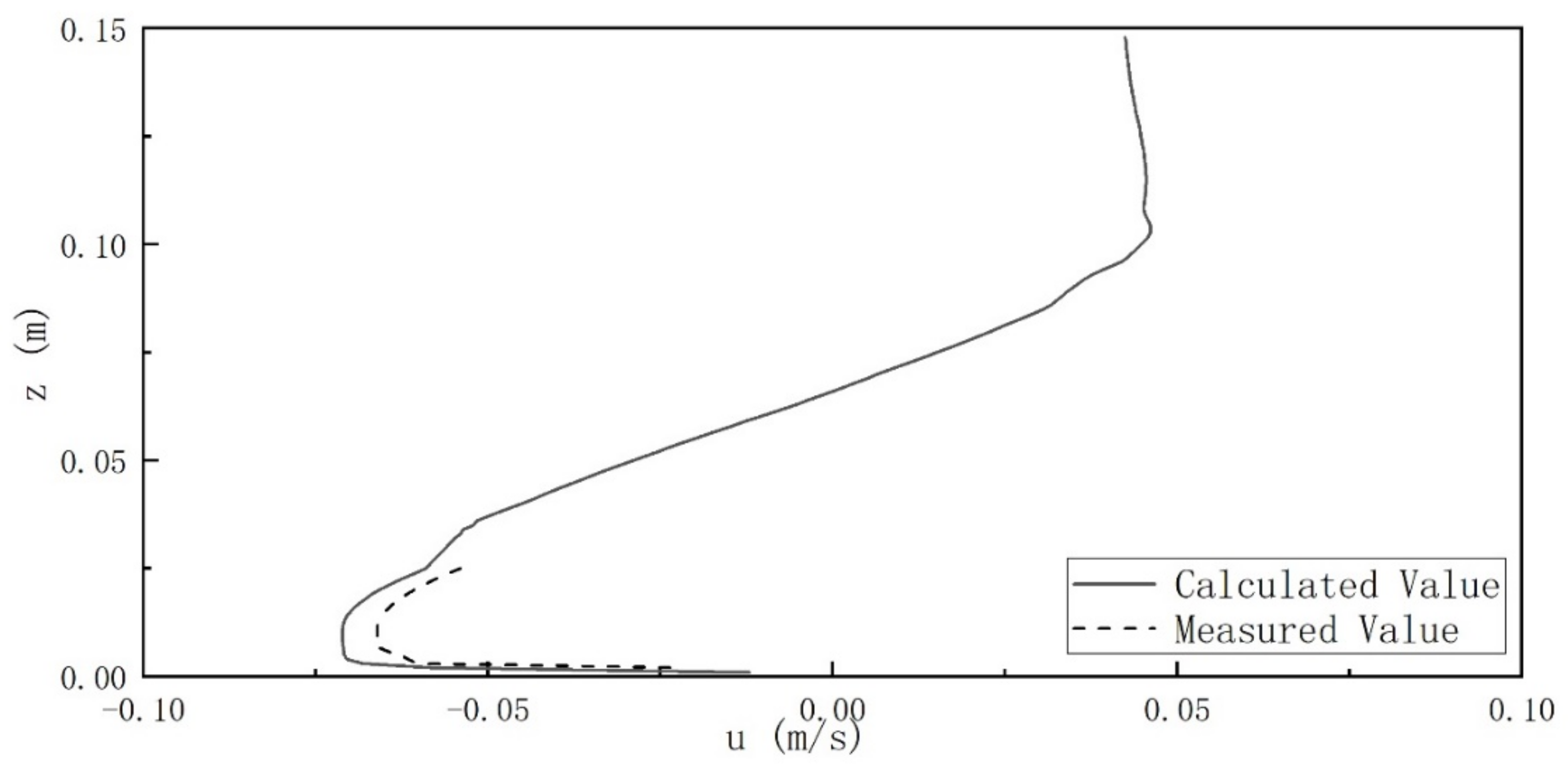
In the physical tank experiment, the maximum velocity measured at x = −1 m was 0.063 m/s, and the average velocity of the section was 0.056 m/s. Figure 3 shows the section average velocity at x = −1 m in the numerical model under this working condition. The peak velocity was at t = 32 s. At that time, the front end of the salt tide intrusion moved to x = −1.3 m, and then the velocity stabilized at about 0.05 m/s. Under the condition of no runoff and no tide, the comparison between the experimental value measured by the physical tank experiment at x = −1 m and the vertical distribution of velocity calculated by the numerical model is shown in Figure 4. Notably, the direction was positive toward the saline area. The maximum velocity measured by the numerical calculation was 0.071 m/s; maximum velocity measured by the physical tank was 0.063 m/s; absolute error was 0.008 m/s; and relative error was 12.7%. The absolute error of the average velocity at the measuring point was 0.002 m/s, and the relative error was 3.6%. It can be observed that the errors were relatively small. The average cross-sectional velocity at the front end of the salt tide intrusion was 0.058 m/s. Compared with the values calculated by the above-mentioned empirical Equations (5) and (6), the relative errors were 7.4% and 13.7%, respectively. Empirical Equations (5) and (6) were obtained from the flume experiment, which had a model with a length of 4 m and a water depth of 0.2 m. The main reason for the error may be that the flume of the physical model used in this study is long, and the influence of the wall is small; thus, there are some gaps in the hydrodynamic factors.

3.1.3. Analysis of Saline Water Intrusion Distance and Head Hydrodynamics

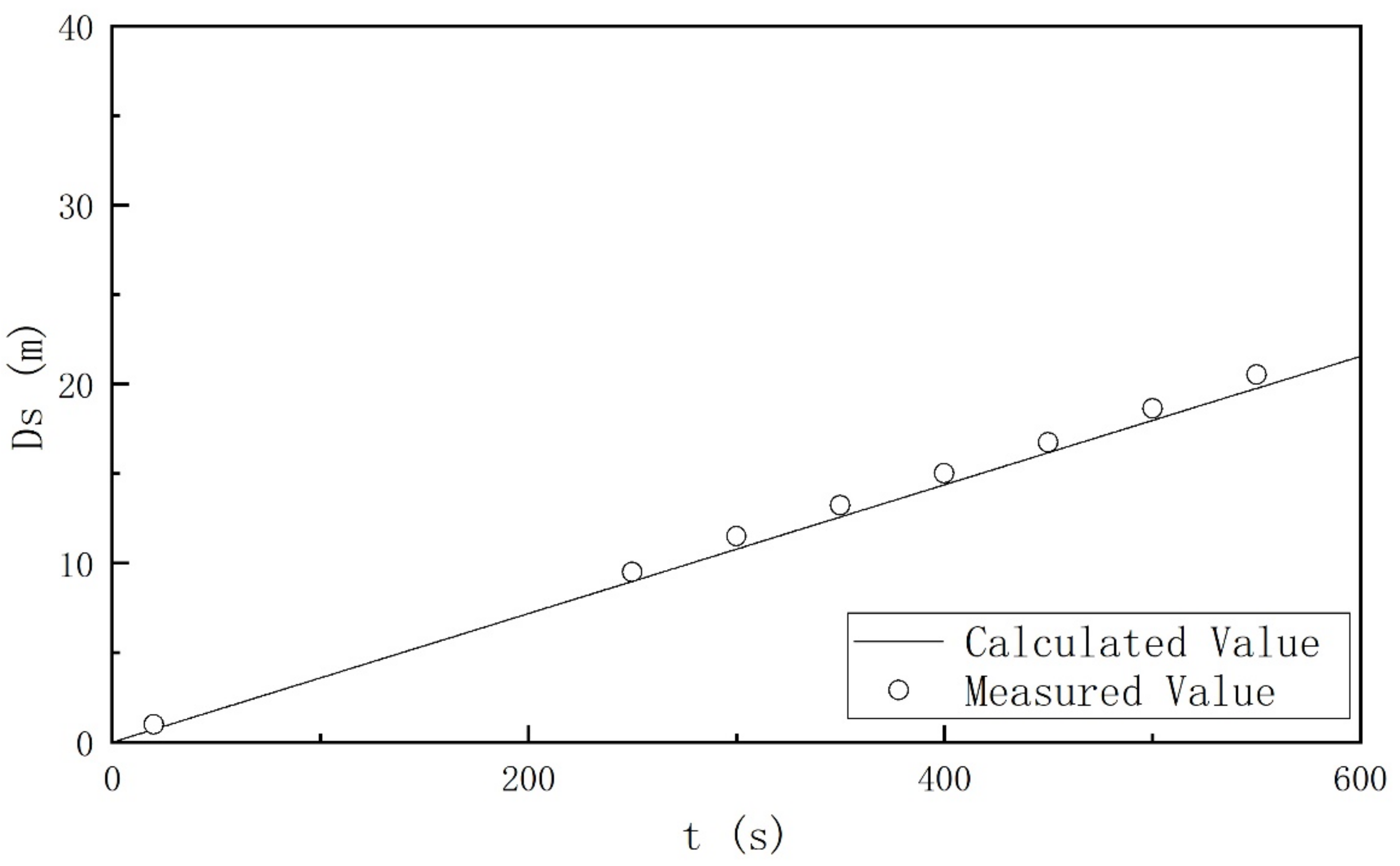
Under the condition of no runoff and no tide, after pulling the division plate, under the action of the density gradient, freshwater flowed to the saline area in the upper layer, whereas saltwater was in the lower layer and flowed to the freshwater area. Under this working condition, the numerical simulation value of the brine intrusion distance was compared with the actual value measured by the physical tank experiment, as shown in Figure 5. There were certain errors in the figure; absolute error was less than 1.7 m; relative error was less than 19.7%; and, the average relative error was 14.7%.

The calculation equation for the goodness of fit $R^2$ is as follows:

$$R^2=1-\frac{\sum {\left({\eta }_{m,C}-{\eta }_{m,0}\right)}^2}{\sum {\left({\eta }_{m,0}-{\overline{\eta }}_0\right)}^2}$$

(7)

where $\sum {\left({\eta }_{m,C}-{\eta }_{m,0}\right)}^2$ represents the sum of regression squares; $\sum {\left({\eta }_{m,0}-{\eta }_0\right)}^2$ is the sum of total squares; ${\eta }_{m,C}$, ${\eta }_{m,0}$ are the m-th calculated value and the experimental value, respectively; and, ${\overline{\eta }}_0$ is the average of the experimental value. Allen et al. [15] used the same definition to estimate the error rate. Substituting the equation above, $R^2$ is 0.90, indicating that the goodness of fit of the numerical simulation is very good.

Figure 6 shows the salinity distribution under the no-runoff and no-tide condition at t = 600 s. After the division plate was pulled out, it moved forward to the bottom under the action of the salinity gradient. Furthermore, the height of the front end of the saltwater intrusion head decreased to a certain extent, strong vertical mixing occurred at the front edge, and the salinity of the water body above the head increased gradually. There was a notable velocity gradient change at the interface between the salt and fresh water, resulting in salt dispersion, while a local circulation occurred at the front of the salt intrusion head, making the salt and fresh water mixing more intense at the front of the salt tide intrusion.

3.2. No-Runoff and Tide Condition

3.2.1. Modeling of the No-Runoff and Tide Condition

By simulating the mixing process of salt and fresh water without runoff and tides, the salinity gradient becomes the main factor. In the estuarine area, both the salinity gradient and the existence of tides will act on the mixing of salt and fresh water, which is also one of the main factors affecting saltwater intrusion. To test the applicability of the model, the saltwater intrusion change must be simulated in the presence of tides; thus, this non-runoff tidal condition was set.

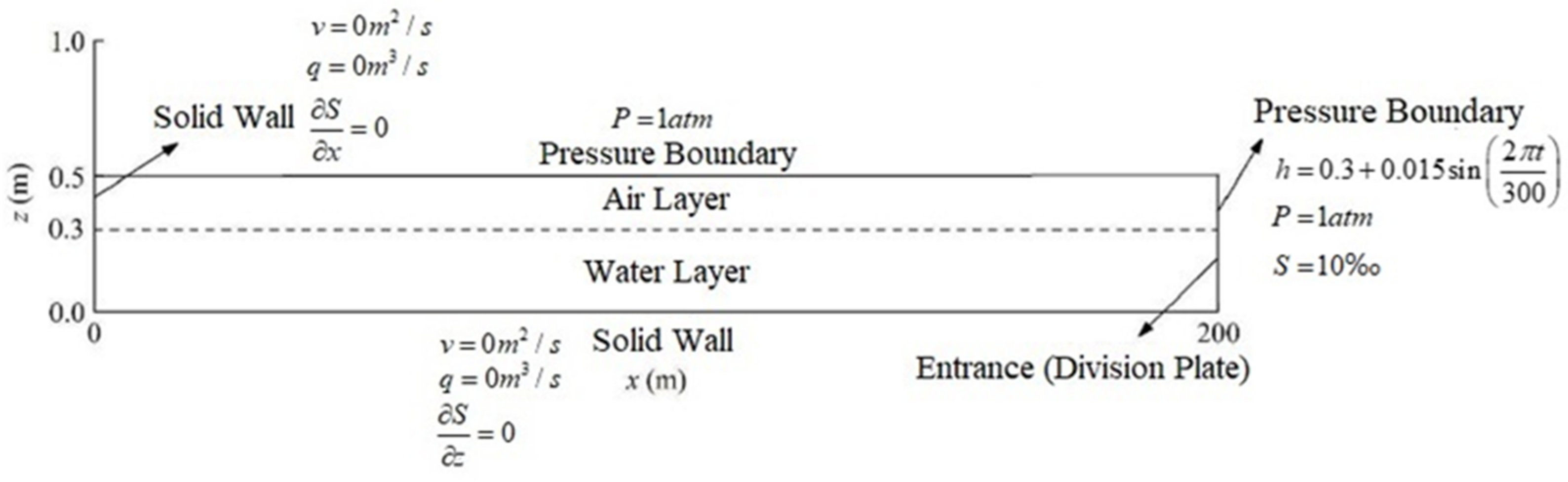
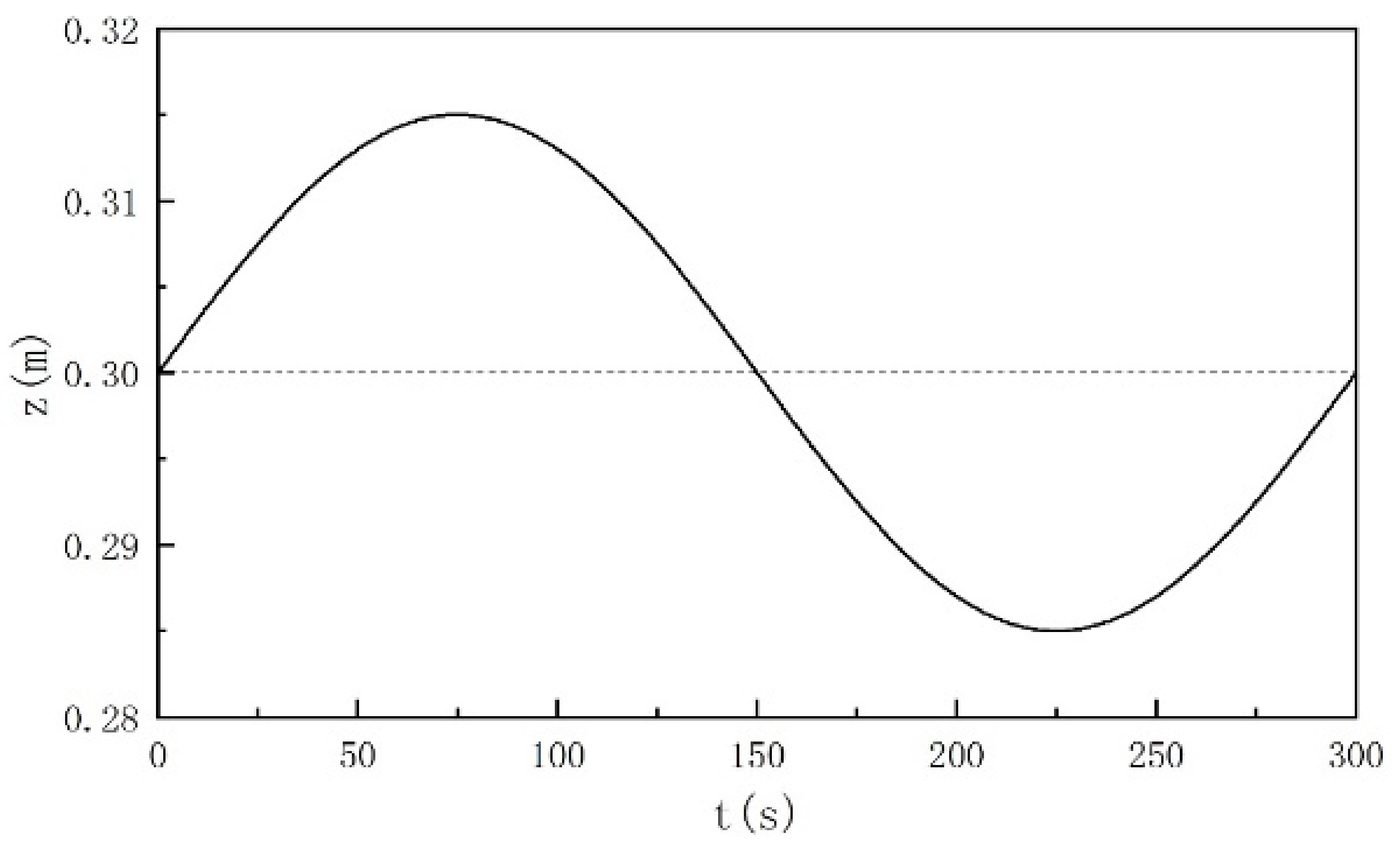
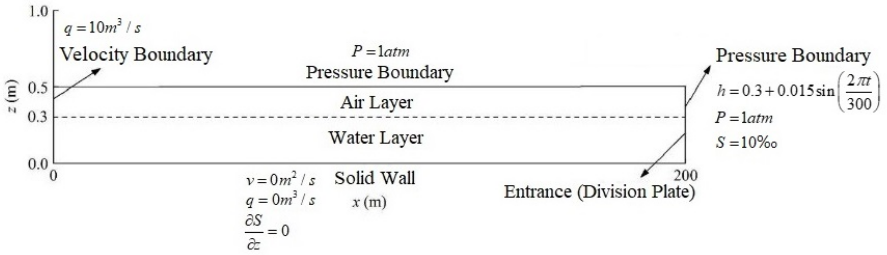
The model calculation area under this working condition is shown in Figure 7. The total length of the tank was 200 m, which was filled with fresh water. The initial water depth was 0.3 m, and there was no inflow or outflow of runoff at the left boundary, which was set as the solid wall boundary. The bottom was also a solid wall boundary, and the top was a pressure boundary under standard atmospheric pressure. The right boundary was the water level boundary condition and the division plate was located 5 m away from the right boundary. The right side of the division plate was saline with salinity (S) measuring 10.9‰. The water level changed according to the sinusoidal tide level curve shown in Equation (8) and Figure 8.

$$h=0.3+0.015\sin \left(\frac{2\pi t}{300}\right)$$

(8)

Under the action of tides, it is necessary to observe the mixing process of the wedge-shaped interface formed by saltwater intrusion and record the impact of the tide level change on the water level in the calculation area. Therefore, under the condition of no runoff and tide, increasing vertical stratification resolution must be carried out in the free water body on the free surface, and the time process of water level change should be recorded accurately. Moreover, the grid resolution of the free surface needs to be high. The grid length in the x-direction is 0.05 m, a total of 5000 grid cells, and the minimum grid length in the vertical direction is 0.0005 m, which comprises approximately 500 layers.

3.2.2. Water Level

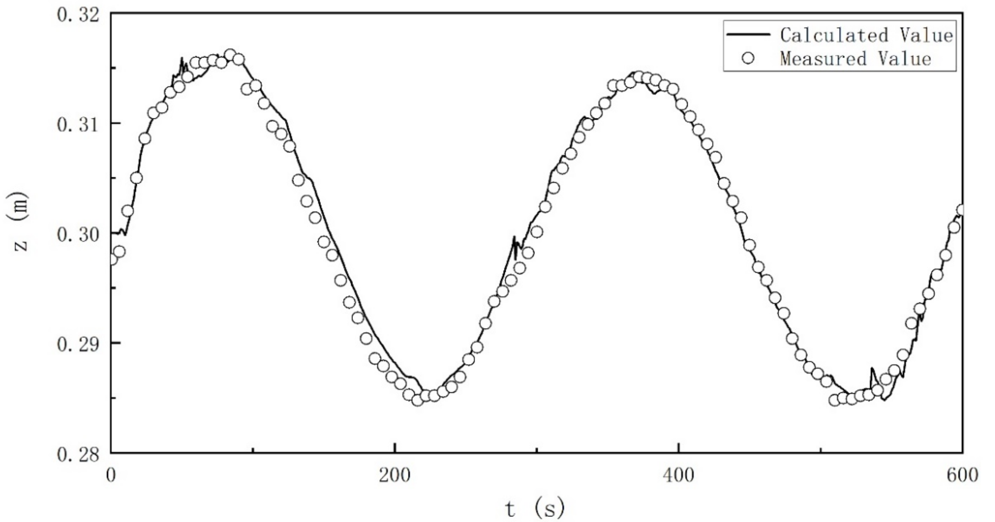
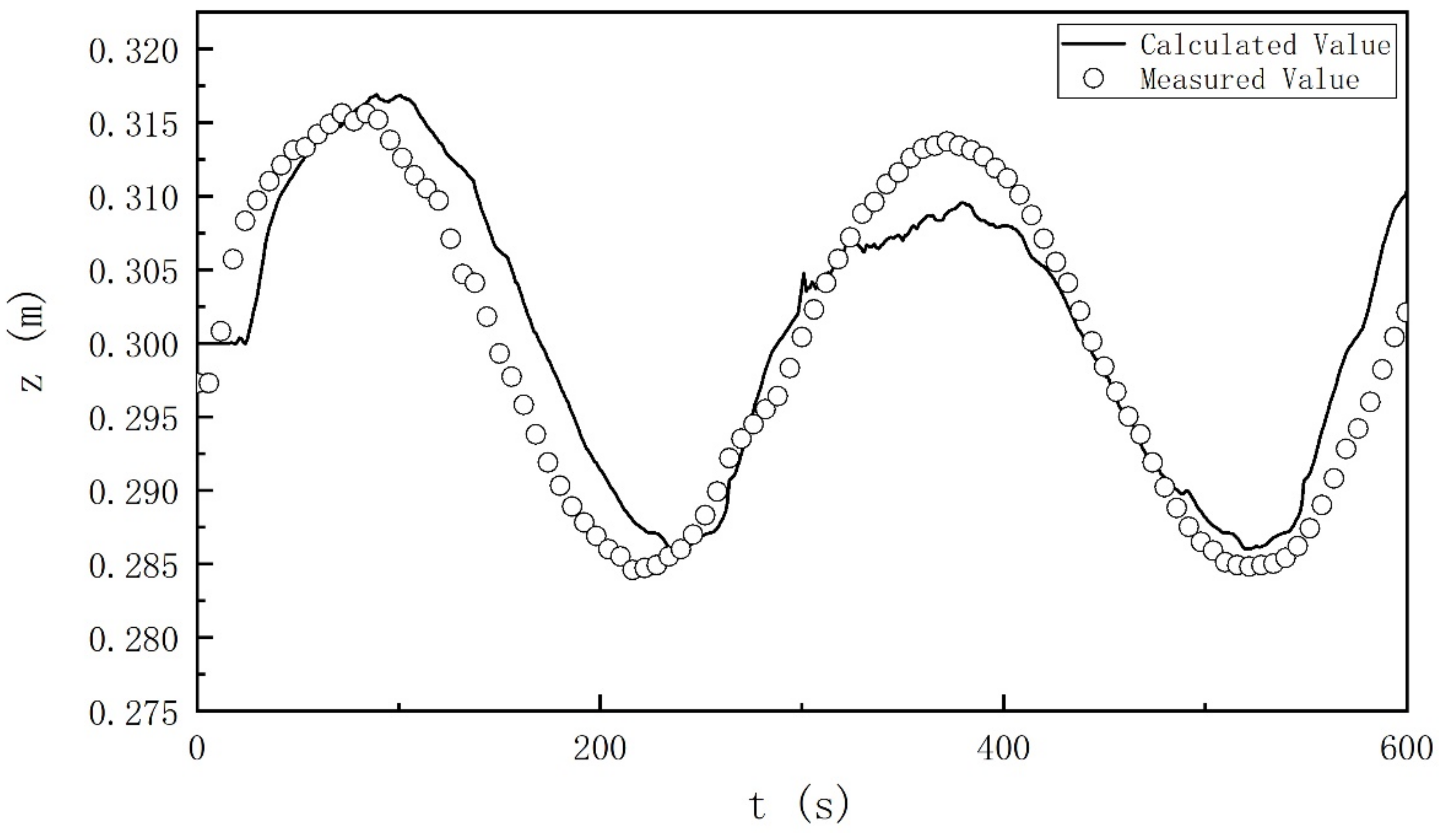
Figure 9 and Figure 10 show the comparison between the water level values of the measuring points at x = 195 m and x = 175 m calculated by numerical simulation and the measured values of the physical tank experiment under the condition of no runoff and tide. It can be seen from the figures that the water level change obtained by the numerical model is consistent with the measured value of the physical experiment. The absolute error between the two was less than 0.005 m. Compared with the tidal range, the relative error was less than 10.1%, and the peak time was consistent. Therefore, the water level results of the numerical simulation were good.

3.2.3. Velocity Distribution

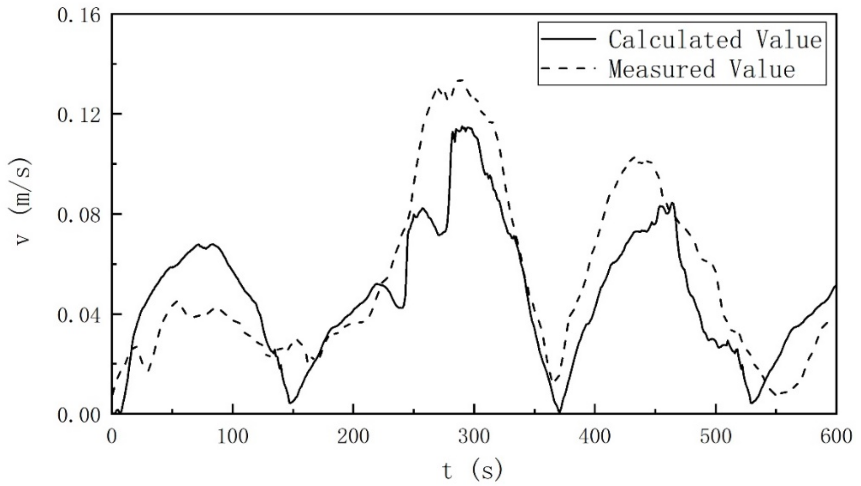
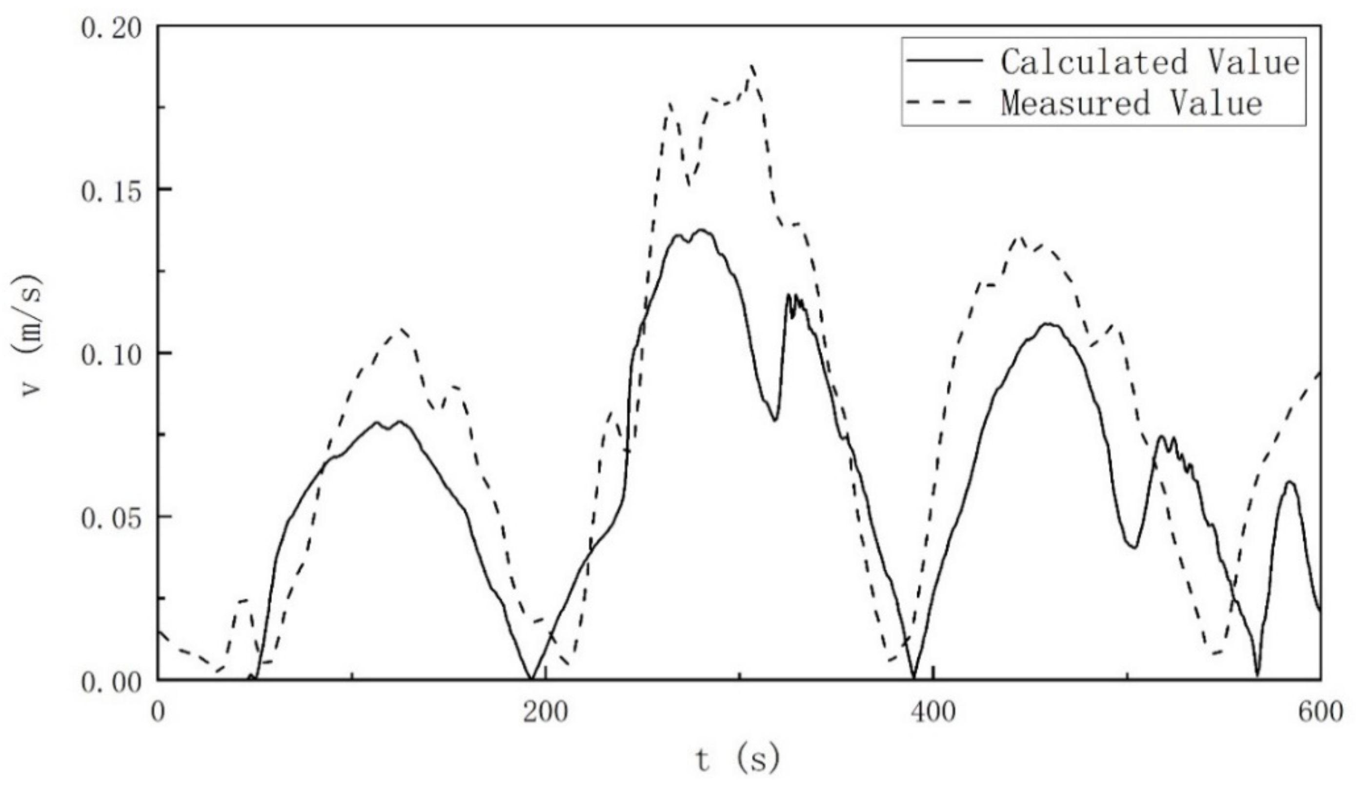
Figure 11 and Figure 12 show the comparison between the numerical simulation calculation value of the average velocity of the section at x = 172 m and x = 139 m and the measured value of the physical tank experiment under the condition of no runoff and tide. Due to the possible interference of other environmental factors on the data from the physical tank model, the influence of the measured value of the physical model was reduced using the Savitzky–Golay filter [16]. The average velocity obtained by the numerical simulation at the measuring point was different from that of the physical tank model. The reason for this is that the total length of the transparent glass tank of the physical model used for observation was only 110 m. Therefore, in the model established by the numerical simulation, to reduce the interference of the distorted channel with the experimental data, the distorted channel was removed, and the straight groove section was extended to 200 m; this led to a deviation in how the fixed wall influenced the flow velocity. This is the reason why the further from the door the monitoring point, the greater the numerical error. Moreover, some sudden changes in the data can be seen in the figures. The reason for the numerical oscillations may be the boundary setting problem or the reflection problem caused by the change in water level, which needs to be analyzed and verified in follow-up research work. It cannot be solved at this stage.

3.2.4. Intrusion Distance and Front-End Hydrodynamic Analysis

Under this working condition, a comparison of the saltwater intrusion distance between the numerical model and the physical tank experiment is shown in Figure 13. The absolute error was less than 3.44 m; relative error was less than 18.1%; and average error was 11.9%. Compared with the intrusion distance under the condition of no runoff and no tide, the advance distance and speed of the saltwater were significantly longer and faster, respectively. It can be seen that tides play a significant role in the mixing process of salt and fresh water, making saltwater intrusion more intense. Calculated using Equation (7), the goodness of fit $R^2=0.87$ is greater than 0.65, indicating that the simulation results of the numerical model are in agreement with the results of the physical flume experiment.

Figure 14 shows the salinity distribution under the condition of no runoff and tide at t = 600 s. Tidal fluctuations change the advance distance of saltwater intrusion, sometimes forward and sometimes backward. Compared with the no-runoff and no-tide condition, it is affected by the salinity gradient and the tide. The mixing process of salt and fresh water at the front end was more complex, and the flow rate of saltwater was faster. It can be seen that tide was one of the main influencing factors in the upward movement of the salt tide. Under the condition of no runoff and no tide, the interface between salt and fresh water was smooth, whereas, under the condition of no runoff and tide, the interface between salt and fresh water was undulating and wavy. When saltwater invades upward, circulation occurs at the front end, resulting in a velocity difference between salt and fresh water. This subsequently leads to tumbling, strong dispersion, and strengthening of the mixing between salt and fresh water. In the saltwater retreating stage, the vertical active mixing between salt and fresh water subsides.

3.3. Condition of Runoff and Tides

3.3.1. Modeling of the Condition of Runoff and Tides

This is similar to the condition of no runoff and tide, but there is runoff at the upstream boundary. The pressure boundary was adopted as the top boundary. The pressure was constant as the standard atmospheric pressure, and the sinusoidal tide level under the condition of no runoff and tide was also adopted as the downstream boundary. The water level boundary condition was adopted as the upstream; flow on the left side of the upstream division plate was constant as 10 m³/s; and, the initial water depth of the water body area in the tank was 0.3 m, filled with salt-free fresh water. Furthermore, the initial flow rate was 0 m/s, and the salinity of the saltwater entering the right side of the downstream division plate was constant as S = 10‰.

The numerical model of the runoff and tide condition is shown in Figure 15. The sinusoidal expression of the downstream tide level under this working condition was the same as that under the previous working condition. The water level in the calculation area rose and fell according to the semi-diurnal tide sine curve. Considering the influence of upstream water on salinity, to better simulate the wedge interface of salt and fresh water, the grid resolution of the vertical natural water body, especially near the free surface, was also increased, which is similar to the previous working condition.

3.3.2. Water Level

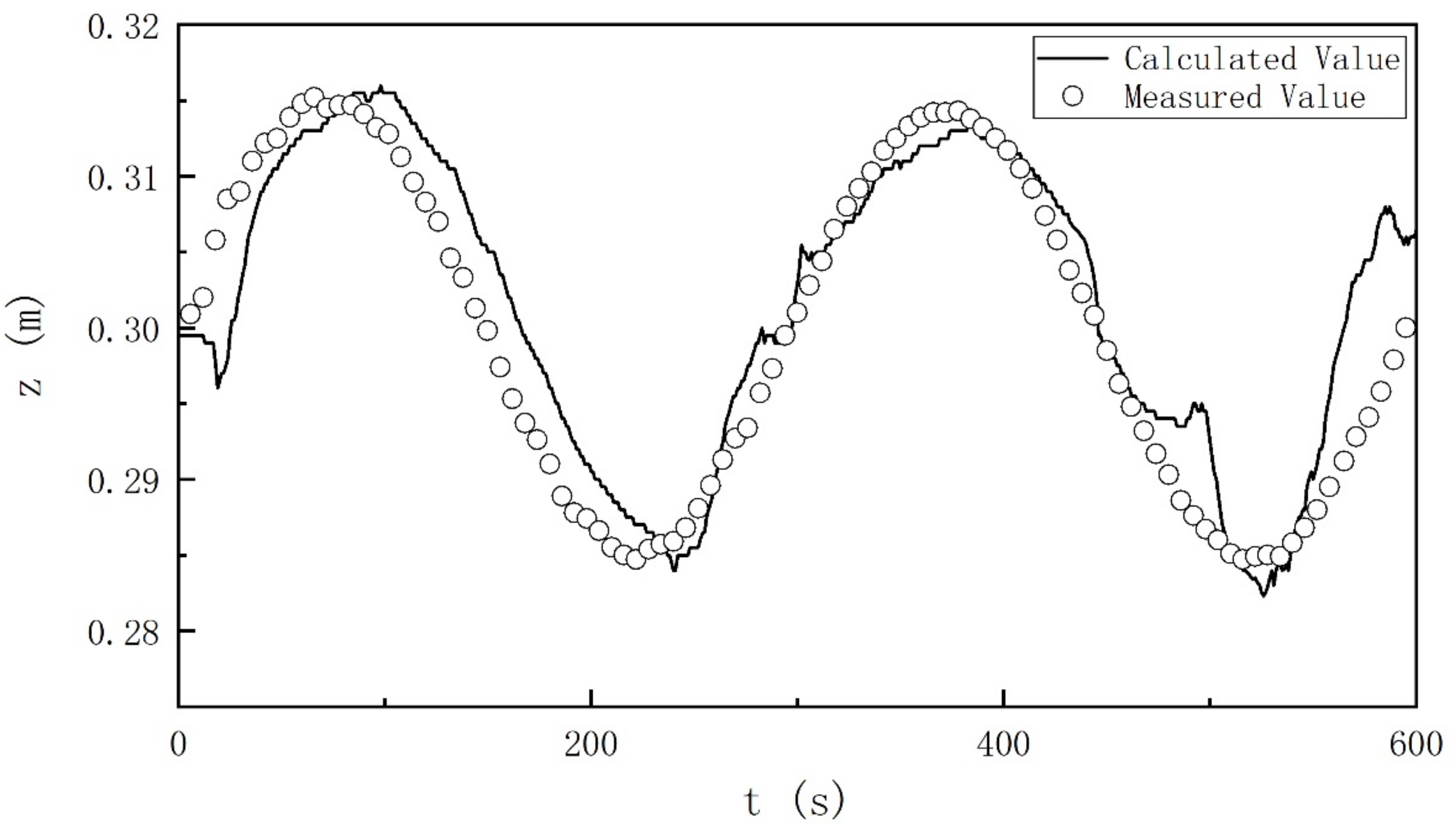
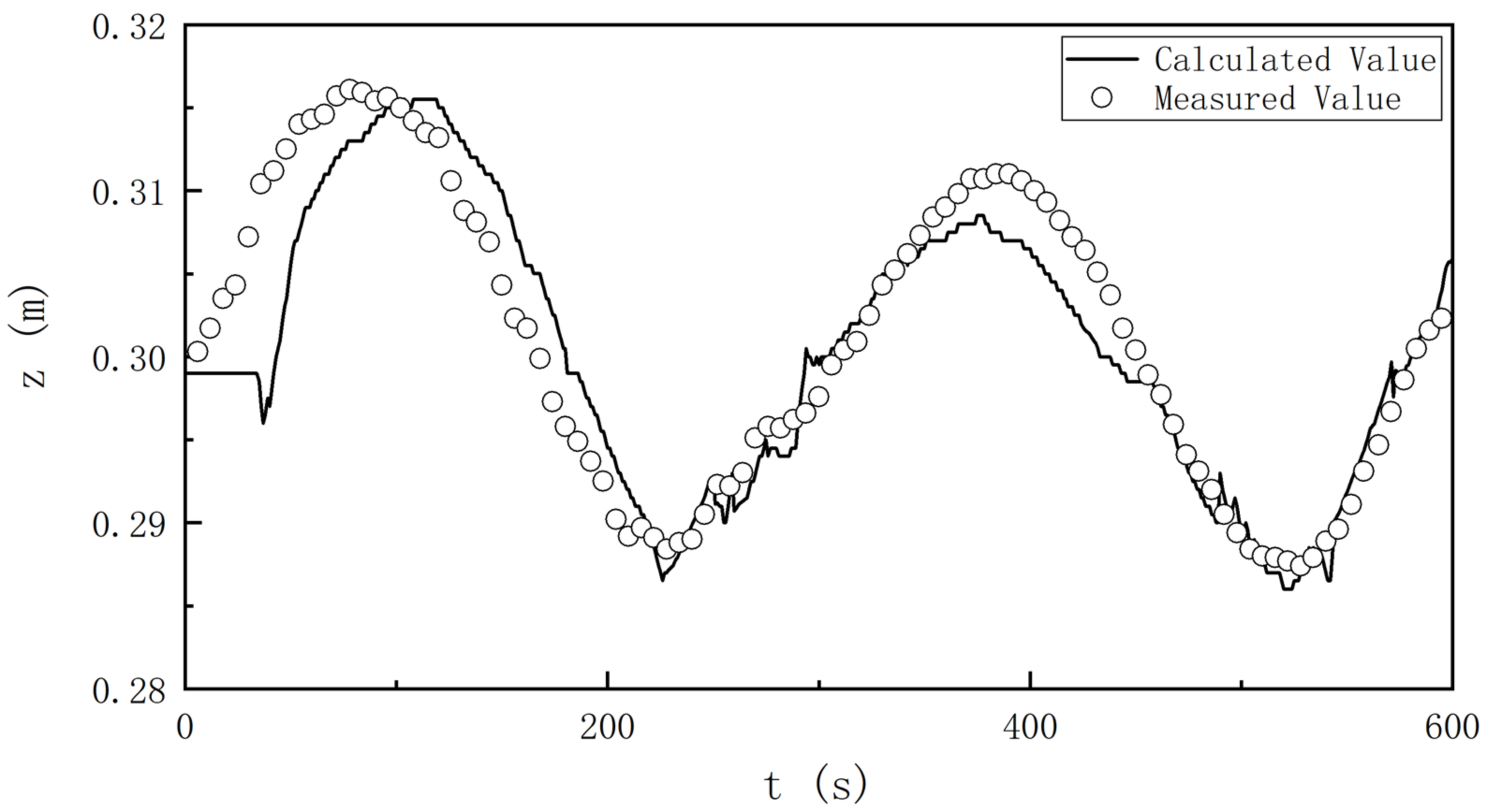
Under the condition of runoff and tide, the comparison of the water level values of the measuring points at x = 175 m and x = 150 m between the numerical simulation and the physical tank experiment is shown in Figure 16 and Figure 17. The variation in the water level obtained by the numerical model was consistent with the measured value of the physical experiment, but there were fluctuations at some peaks and troughs. The absolute error of the two was less than 0.006 m. Compared with the tidal range, the relative error was less than 10.3%.

3.3.3. Velocity Distribution

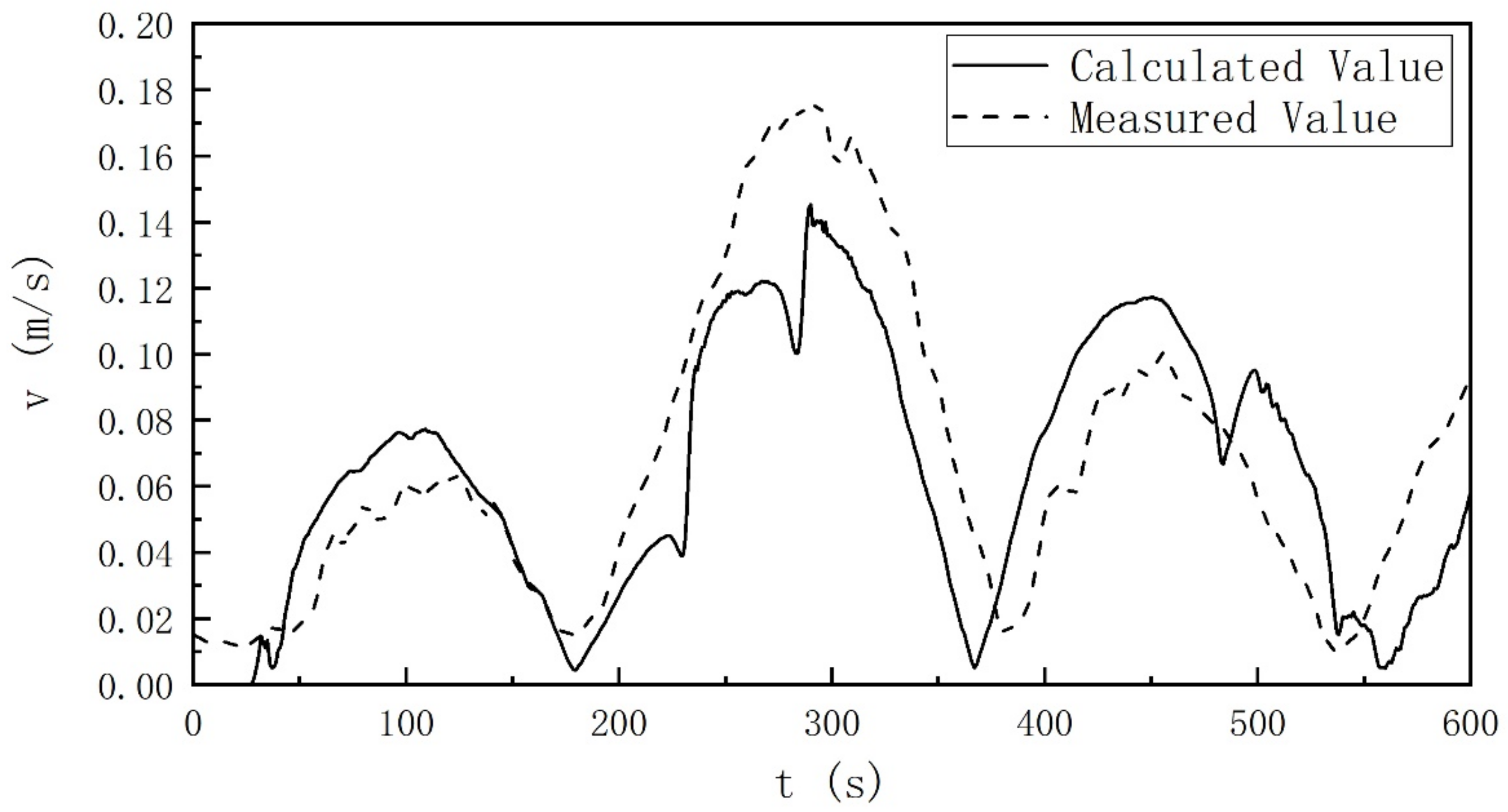
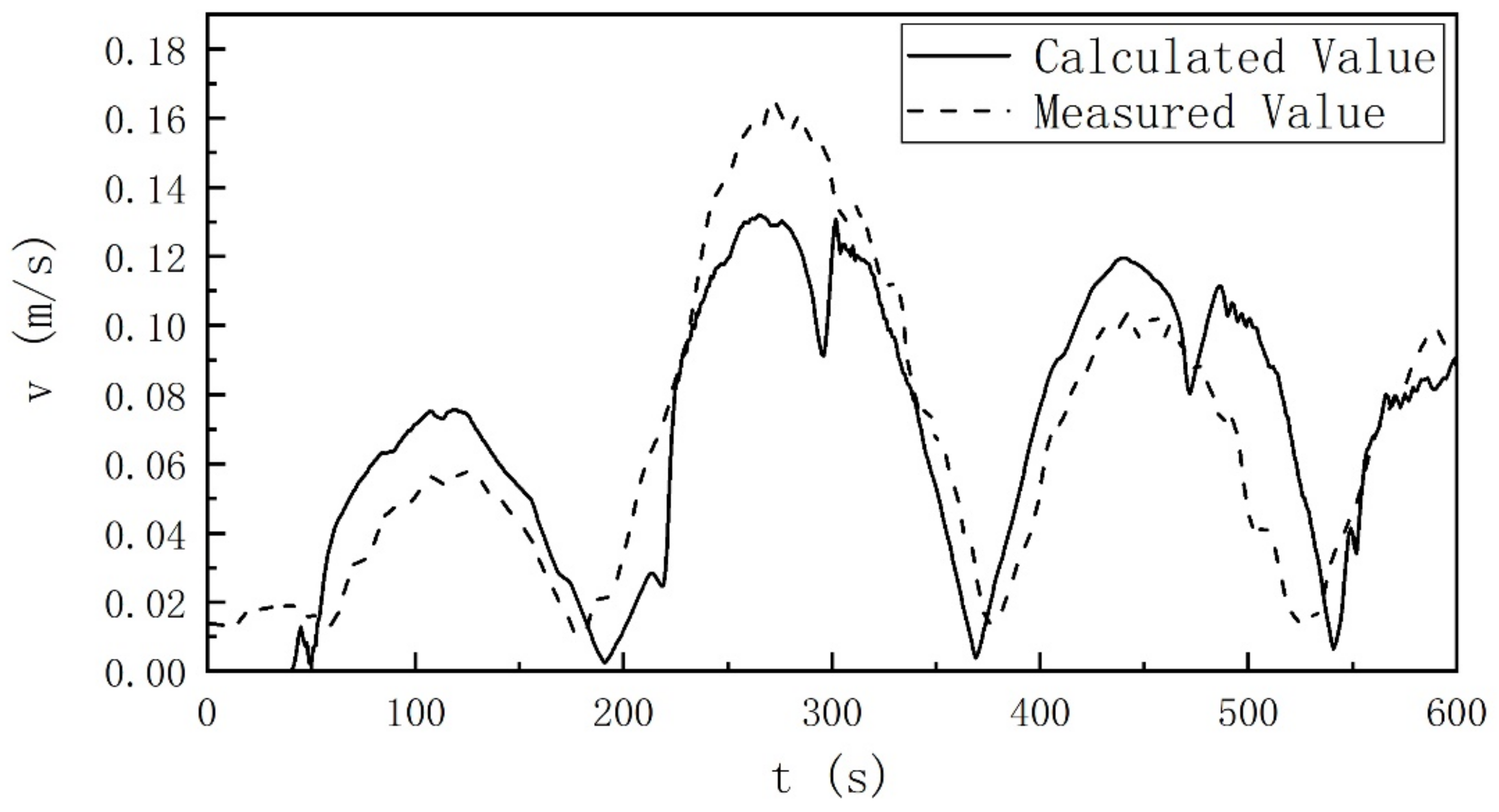
Under the condition of runoff and tide, the comparison of the sectional average velocity of the measuring points at x = 157 m and x = 139 m between the numerical simulation and the physical experiment is shown in Figure 18 and Figure 19. Similar to the previous working condition, the influence was also reduced using the Savitzky–Golay filter [16]. At the two monitoring points of flow velocity, the variation trend of the numerical calculation results of the flow velocity was consistent with that of the experimental data. As in the previous working condition, owing to the existence of a twisted water channel in the physical water tank, in the numerical calculation, the twisted water channel was removed, and the straight channel section was elongated to reduce the influence. The calculated results deviated from the experimental results. In addition, numerical oscillations also occurred, and a brief analysis was discussed under the previous condition.

3.3.4. Intrusion Distance and Front-End Hydrodynamic Analysis

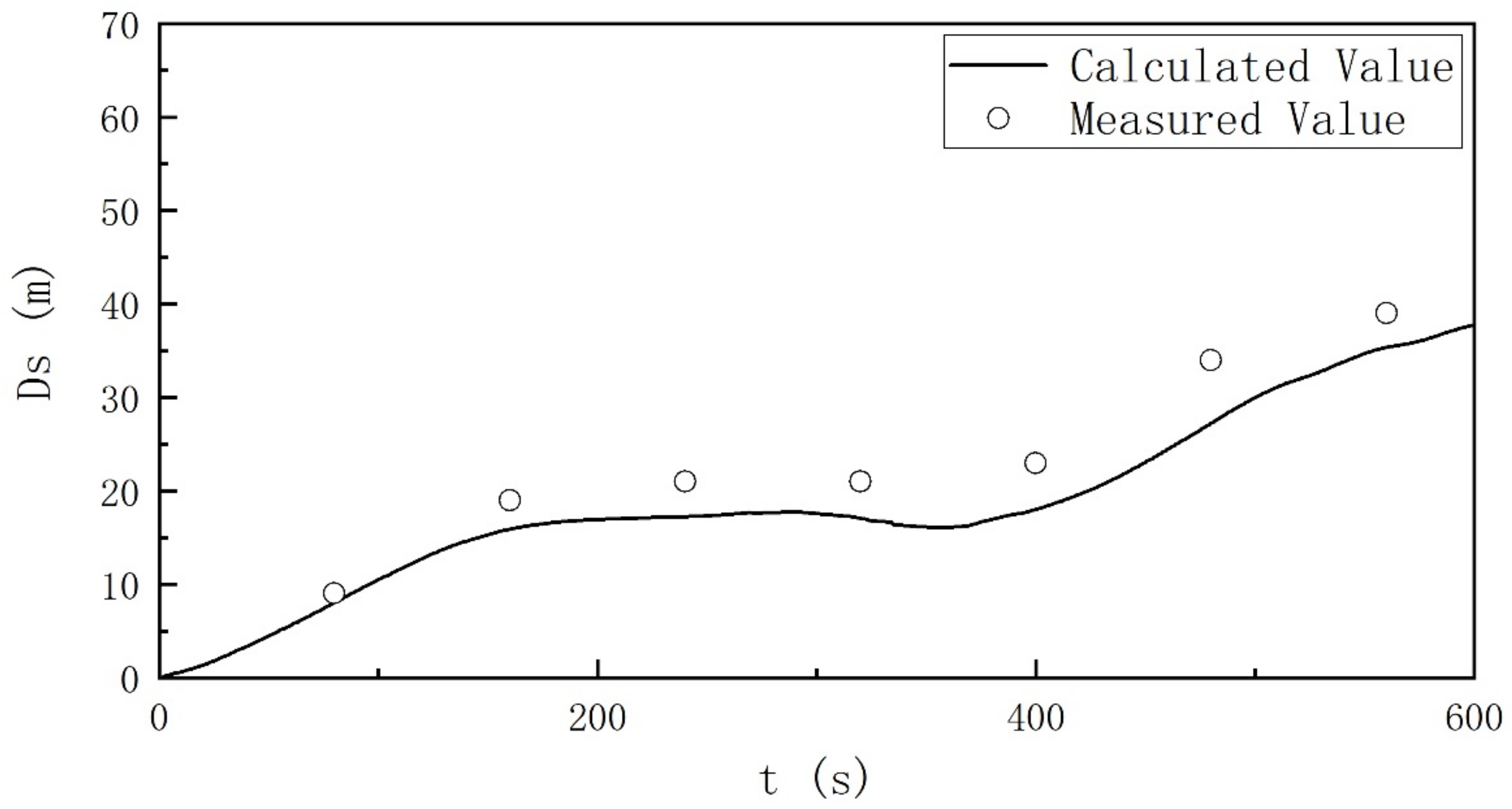
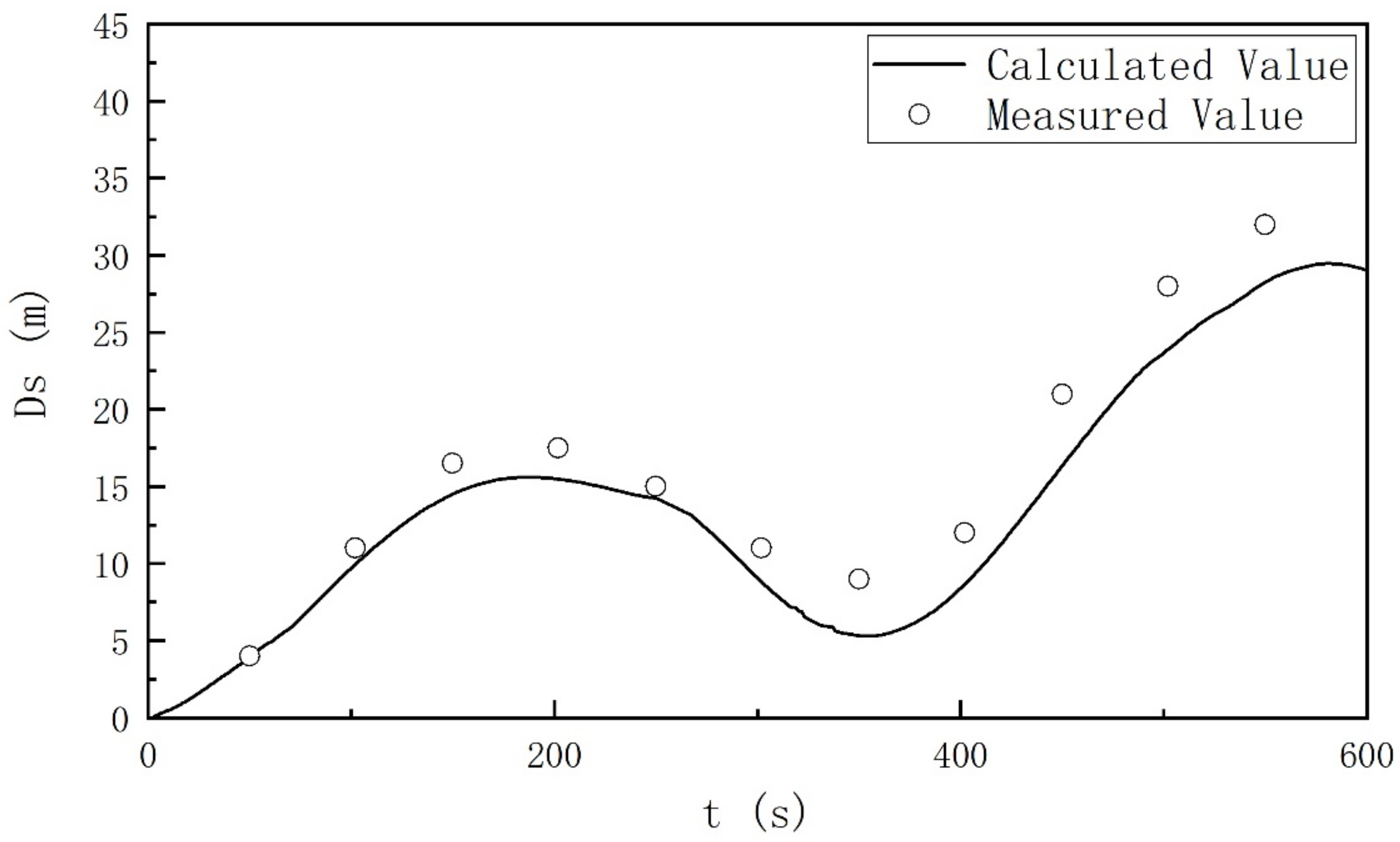
Under this working condition, the comparison between the saltwater intrusion distance obtained by the numerical model and the measured value of the physical flume experiment is shown in Figure 20. The absolute error was less than 3.80 m; relative error was less than 19.8%; and average error was 15.3%. Compared with the first two working conditions, under the joint action of runoff and tide, saltwater has both forward and backward movements, which is more complex. Calculated using Equation (7), the goodness of fit $R^2=0.76$ is greater than 0.65, indicating that the simulation results of the numerical model are in agreement with the results of the physical experiment. The figure shows that the saltwater intrusion distance presents a certain periodicity and reaches dynamic stability in the cycle.

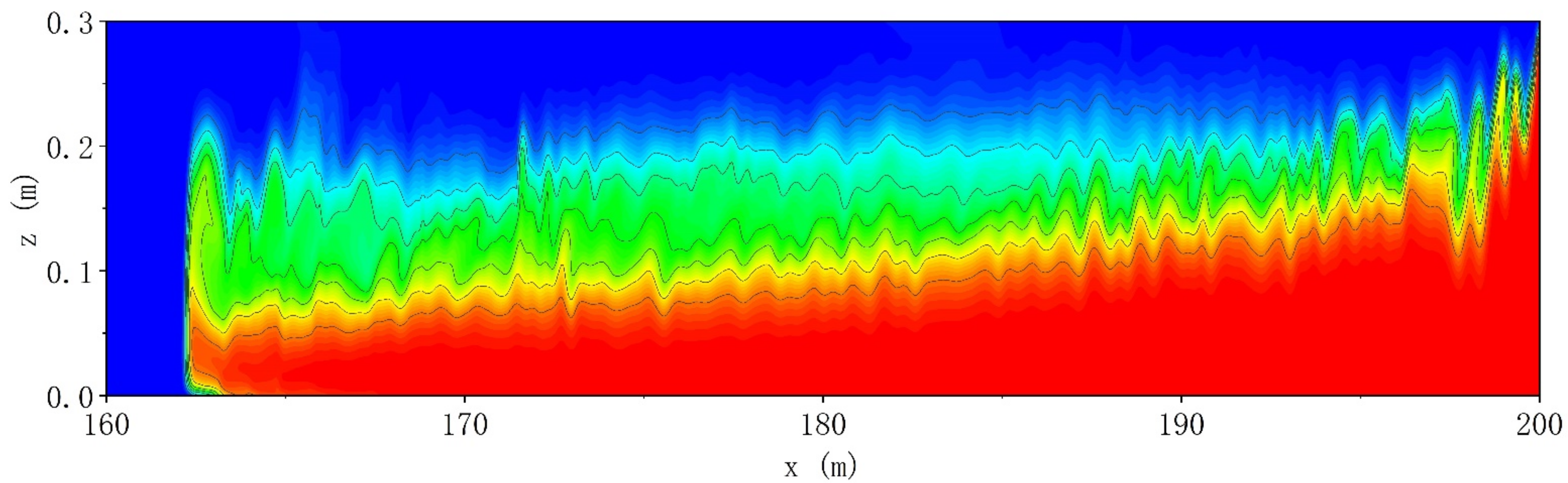
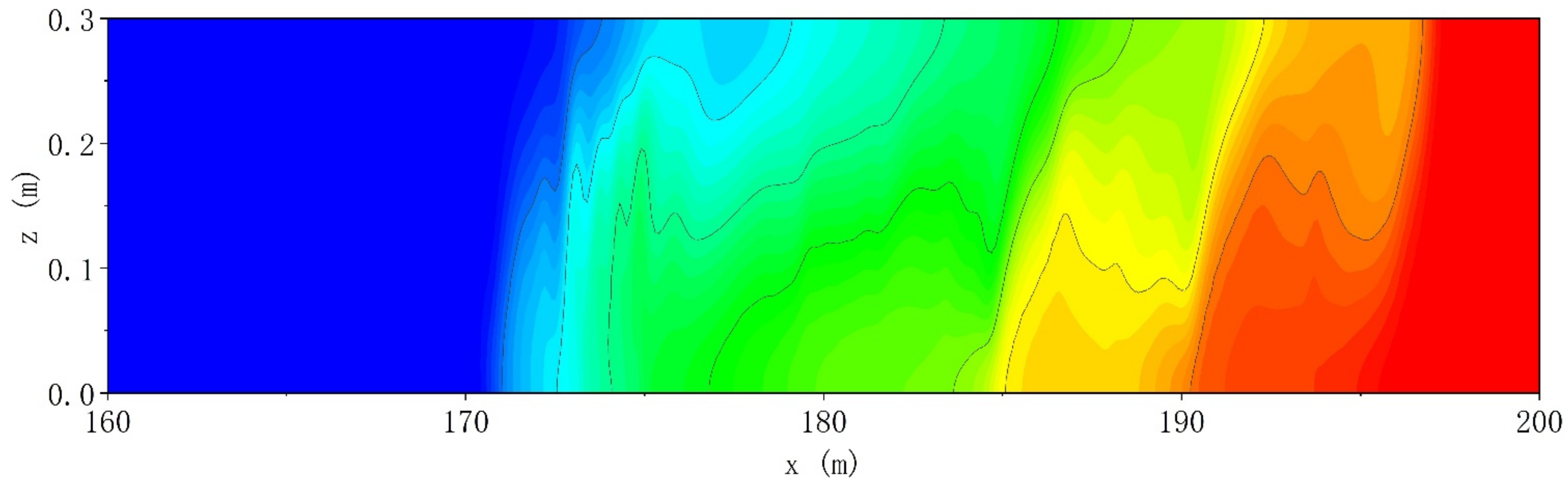
Figure 21 shows the salinity distribution under the condition of runoff and tides at t = 600 s. Under the joint action of tidal currents and runoff, saltwater advances and retreats to a dynamic equilibrium state within a certain period. Compared with the condition of no runoff and tide, the advance speed of saltwater intrusion is much slower, indicating that runoff is the fundamental factor inhibiting saltwater intrusion. Under the condition of no runoff and tide, the interface between salt and fresh water has strong tumbling, and the velocity gradient changes significantly. Under the condition of runoff and tide, the interface between salt and fresh water is relatively flat, velocity gradient changes little, and mixing range of salt and fresh water increases. In the saltwater advance stage, the circulation at the front edge of the saltwater intrusion head is stronger than that in the saltwater retreat stage, and the saltwater intrusion head is always maintained near the water outlet, which is much slower than that in the case of no runoff and tide.

4. Conclusions

(1)

A very-high-resolution mathematical model of saltwater intrusion movement in estuary areas was established, which was verified by comparison with a physical flume experiment. The model was divided into 4000 grids in the horizontal direction and 500 layers in the vertical direction. The mixing of salt and fresh water at the interface of salt and fresh water, under the combined action of tide, salinity gradient, and runoff, and the intrusion of saltwater were simulated with reasonable accuracy.

(2)

The numerical simulation of the mixing of salt and fresh water with no runoff and no tide shows that because of the influence of no external dynamic factors, the interface between salt and fresh water is wedge-shaped. Furthermore, there is a large velocity gradient change at the interface between salt and fresh water, and local circulation occurs at the front edge of the head of the saltwater intrusion, which makes the mixing of salt and fresh water more intense at the front end of saltwater intrusion.

(3)

The numerical simulation of the mixing process of salt and fresh water with no runoff and tide shows that the interface between salt and fresh water undulates, which is different from the smooth interface between salt and fresh water under the condition of no runoff and no tide. When the saltwater intrudes upward, the front part circulates and rolls, resulting in strong dispersion and strengthening the mixing between salt and fresh water. In the saltwater retreating stage, the vertical active mixing between salt and fresh water subsides.

(4)

The numerical simulation of the mixed movement process of salt and fresh water with runoff and tide shows that the speed of saltwater intrusion is much slower than that under the condition with no runoff and tide, indicating that runoff is the fundamental factor inhibiting saltwater intrusion. It also suggests that the interface between salt and fresh water is relatively gentle; change in the velocity gradient is small; and the mixing range of salt and fresh water becomes larger. Under the combined action of upstream runoff, downstream tide, and salinity gradient, the saltwater intrusion distance reaches a dynamic and stable state within a period of time.

(5)

There are many sudden changes in the simulation results, which may be caused by numerical oscillations. The reason may be the boundary setting problem or the reflection problem caused by the change in water level, which needs to be analyzed and verified. It cannot be solved at this stage, and further work will be conducted at the next stage to solve this problem.

References

- Krvavica, N.; Ružić, I. Assessment of sea-level rise impacts on salt-wedge intrusion in idealized and Neretva River Estuary. Estuar. Coast. Shelf Sci. 2020, 234, 106638. [Google Scholar] [CrossRef] [Green Version]
- Zhang, D.; Yang, Y.; Wu, J.; Zheng, X.; Liu, G.; Sun, X.; Lin, J.; Wu, J. Global sensitivity analysis on a numerical model of seawater intrusion and its implications for coastal aquifer management: A case study in Dagu River Basin, Jiaozhou Bay, China. Appl. Hydrogeol. 2020, 28, 2543–2557. [Google Scholar] [CrossRef]
- Hu, X. Numerical Study of Saltwater Intrusion in Modaomen of Pearl Estuary. Master’s Thesis, Tsinghua University, Beijing, China, 2010. (In Chinese). [Google Scholar]
- Liu, Z.; Shi, N.; Guan, S.; Lin, Y.; Zhang, J.; Zhuo, W. Three-dimensional numerical simulation of saltwater intrusion in Modaomen estuary based on FVCOM. J. Hydrodyn. 2016, 31, 286–294. (In Chinese) [Google Scholar]
- Liu, Z.; Guan, S.; Zhang, J.; Ding, B.; Lin, Y.; Zha, X. Three-dimensional numerical simulation of saltwater intrusion into the Humen estuary based on FVCOM. J. Trop. Oceanogr. 2016, 35, 10–18. (In Chinese) [Google Scholar]
- Cheng, P.; De Swart, H.E.; Valle-Levinson, A. Role of asymmetric tidal mixing in the subtidal dynamics of narrow estuaries. J. Geophys. Res. Oceans 2013, 118, 2623–2639. [Google Scholar] [CrossRef] [Green Version]
- Zheng, S.; Cai, S. A Model Study of the Effects of River Discharges and Interannual Variation of Winds on the Plume Front in Winter in Pearl River Estuary. Pearl River 2017, 38, 1–9. (In Chinese) [Google Scholar] [CrossRef]
- Lyu, Z.; Feng, J.; Gao, X.; Wang, Y.; Zhang, M.; Kong, J. Estuarine circulation and mechanism of mixing and stratification in the Modaomen Estuary. Adv. Water Sci. 2017, 28, 908–921. (In Chinese) [Google Scholar]
- Bao, Y.; Ren, J. Simulation of Salinity Stratification in Zhujiang River Estuary Using Modified Salinity Numerical Forma. J. Trop. Oceanogr. 2001, 20, 28–34. (In Chinese) [Google Scholar]
- Kim, S.-Y.; Kim, K.-M.; Park, J.-C.; Jeon, G.-M.; Chun, H.-H. Numerical simulation of wave and current interaction with a fixed offshore substructure. Int. J. Nav. Arch. Ocean Eng. 2016, 8, 188–197. [Google Scholar] [CrossRef] [Green Version]
- Gerhart, P.M.; Gross, R.J.; Hochstein, J.I. Fundamentals of Fluid Mechanics; Addison-Wesley Pub. Co.: Boston, MA, USA, 1992. [Google Scholar]
- Zhang, P.; Yin, X.; Zhao, X.; Jiang, L.; Zeng, Y. Experimental Study on Estuary Salt Water Intrusion Length with Runoff and Tide and Its Variation Law. Water Resour. Power 2016, 34, 60–64. (In Chinese) [Google Scholar]
- Benjamin, T.B. Gravity currents and related phenomena. J. Fluid Mech. 1968, 31, 209–248. [Google Scholar] [CrossRef]
- Turner, J.S.; Benton, E.R. Buoyancy Effects in Fluids. Phys. Today 1974, 27, 52. [Google Scholar] [CrossRef]
- Allen, J.; Somerfield, P.; Gilbert, F. Quantifying uncertainty in high-resolution coupled hydrodynamic-ecosystem models. J. Mar. Syst. 2007, 64, 3–14. [Google Scholar] [CrossRef]
- Chen, J. A simple method for reconstructing a high-quality ndvi time-series data set based on the savitzky–golay filter. Remote Sens. Environ. 2004, 91, 332–344. [Google Scholar] [CrossRef]
Figure 1.
Top view of schematic of the physical experiment.
Figure 2.
Schematic of the calculation area under the no-runoff and no-tide condition.
Figure 3.
Average velocity of the saltwater at x = −1 m under the no-runoff and no-tide condition.
Figure 4.
Vertical distribution of the maximum flow rate at x = −1 m under the no-runoff and no-tide condition.
Figure 5.
Comparison of the saltwater intrusion distance under the no-runoff and no-tide condition.
Figure 6.
Distribution of salinity during the saltwater intrusion at t = 600 s under the no-runoff and no-tide condition.
Figure 7.
Schematic of the calculation area under the no-runoff and tide condition.
Figure 8.
Change curve of the downstream boundary water level under the no-runoff and tide condition.
Figure 9.
Water level change chart at x = 195 m under the no-runoff and tide condition.
Figure 10.
Water level change chart at x = 175 m under the no-runoff and tide condition.
Figure 11.
Change chart of the average flow rate at x = 172 m under the no-runoff and tide condition.
Figure 12.
Change chart of the average flow rate at x = 139 m under the no-runoff and tide condition.
Figure 13.
Comparison of the saltwater intrusion distance under the no-runoff and tide condition.
Figure 14.
Distribution of salinity during the saltwater intrusion at t = 600 s under the no-runoff and tide condition.
Figure 15.
Schematic of the calculation area under the runoff and tide condition.
Figure 16.
Water level change chart at x = 175 m under the runoff and tide condition.
Figure 17.
Water level change chart at x = 150 m under the runoff and tide condition.
Figure 18.
Change chart of average flow velocity at x = 157 m under the runoff and tide condition.
Figure 19.
Change chart of average flow velocity at x = 139 m under the runoff and tide condition.
Figure 20.
Comparison diagram of the saltwater intrusion distance under the runoff and tide condition.
Figure 21.
Distribution of salinity during the saltwater intrusion at t = 600 s under the runoff and tide condition.
Publisher’s Note: MDPI stays neutral with regard to jurisdictional claims in published maps and institutional affiliations. |
© 2022 by the authors. Licensee MDPI, Basel, Switzerland. This article is an open access article distributed under the terms and conditions of the Creative Commons Attribution (CC BY) license (https://creativecommons.org/licenses/by/4.0/).
Share and Cite
MDPI and ACS Style
Zhao, J.; Zhu, L.; Li, J. Numerical Experiment on Salt Transport Mechanism of Salt Intrusion in Estuarine Area. Water 2022, 14, 770. https://doi.org/10.3390/w14050770
AMA Style
Zhao J, Zhu L, Li J. Numerical Experiment on Salt Transport Mechanism of Salt Intrusion in Estuarine Area. Water. 2022; 14(5):770. https://doi.org/10.3390/w14050770
Chicago/Turabian StyleZhao, Jun, Liangsheng Zhu, and Jianhua Li. 2022. "Numerical Experiment on Salt Transport Mechanism of Salt Intrusion in Estuarine Area" Water 14, no. 5: 770. https://doi.org/10.3390/w14050770
Note that from the first issue of 2016, this journal uses article numbers instead of page numbers. See further details here.