Regression Model Selection and Assessment of Agricultural Water Price Affordability in China

Abstract

The agricultural water price depends on the agricultural water price affordability (AWPA) in each region. This study found that the logarithmic linear model had the best fitting effect through evaluating the grey situation decision model, which considered factors such as rainfall and output value per unit area. The contribution of each influencing factor was determined by the Lindeman–Merenda–Gold method. We established a new model to determine the water expenditure coefficient (WEC) by improving the way that the value of the WEC is assigned. Then, the AWPA in different regions was calculated. The results showed that the WEC was between 2.62% and 12.95%, and the AWPA price was between 0.058 and 0.52 yuan/m³ (0.0084 and 0.075 $/m³). The contribution of precipitation and output was 45.20% and 25.60%, respectively. The WEC and AWPA in northeast, northwest, and northern China are higher than those in southwest and southern China. The AWPA in the Yellow River Basin was higher than that in the Yangtze River Basin; however, the space for adjustment in the Yellow River Basin was slightly smaller than that in the Yangtze River Basin.

1. Introduction

The agricultural water price in China has been low for a long time, and its regional differences are large and the reform of agricultural water prices is lagging behind. One reason for this is that local governments are worried about the impact of price adjustment on people’s livelihood. As the upper limit on water price adjustment, agricultural water price affordability (AWPA) is one of the key factors that must be considered when verifying water prices and water fees. Some countries take affordability into account when pricing. Latinopoulos [1,2] indicated that the pricing for agricultural irrigation water in the eastern United States is “service cost + user affordability”. In the reform of agricultural water prices, France chose the pricing model of “full cost + user affordability” for irrigation water pricing [3]. It is therefore of great importance to promote the reform of agricultural water prices in China and define agricultural water price affordability in order to allay government concerns about price adjustments.

At present, due to differences in the economic development level, planting structure, water use mode, irrigation conditions, income level, and other aspects, water consumers have different capacities to bear water prices. Therefore, when promoting a comprehensive reform of agricultural water price, all localities should conduct a full investigation and, with the help of scientific methods, reasonably evaluate the AWPA, so as to ensure that the newly established agricultural water price does not increase the burden of water users and to ensure the normal development of agricultural production activities [4].

Regarding the definition of AWPA, Wang et al. [5,6,7] believe that AWPA refers to the ability of water users to pay the water price at a certain level, i.e., that their survival and development will not be significantly affected after paying the water price. Liao et al. [8] believe that there is an affordable range or space for farmers to bear the price of irrigation water, and the deciding factor should mainly be the proportion of input costs for irrigation to the cost of agricultural production and production profit. In China, water pricing is generally based on the AWPA of grain crops and the cost of water [9,10].

There are various index analysis methods, econometric methods, questionnaire method for calculating AWPA. The index analysis method investigates farmers’ agricultural production input and output, the proportion of water expenditure in the agricultural production cost, output value, income, and other items in order to assess whether farmers’ water expenditure is affordable to them. In India, the rate for flow irrigation with respect to non-cash crops is fixed roughly at 6% of the gross income from these crops, and about 12% of the gross income in the case of cash crops, as recommended by the Maharashtra State Irrigation Commission. [11]. Nian et al. [9] evaluated the AWPA in Xinjiang based on the proportion of water expenditure in household income and reported that the comprehensive AWPA in Xinjiang was 870 yuan/hm². The econometric method refers to the combination of mathematics and statistics with modern computer technology for establishing an econometric model and quantitatively analyzing the relationship between the economic variables of the research objects with randomness [12]. Yang et al. [13,14] proposed a calculation method for AWPA under dynamic hydrological conditions with the aim of reflecting the dynamic change law of AWPA, applied it in Boai County of Henan Province, and obtained good results. The questionnaire method has been used to investigate the economic behavior of interviewees in the hypothetical market through questionnaires, i.e., to investigate and evaluate the willingness of individuals to pay water charges by issuing questionnaires [15]. Chen et al. [16] used CVM(Contingent Value Method) to investigate and analyze the AWPA in the Wu an irrigation area and reported that the highest acceptable price for water was 960 yuan/hm². Aydogdu et al. [17] analyzed the affordability of water price for farmers in a plain irrigated area in Turkey through a sampling survey and concluded that the farmers’ ability to pay exceeded their willingness to pay.

In order to calculate the AWPA of farmers, the characteristics of the region, economy, agriculture, and water use should be fully considered. However, the above calculation methods are highly subjective in determining the water expenditure coefficient (WEC), as they often use existing results or empirical values at home and abroad, and lack the consideration of local geographical factors, economic conditions, and differences in water use, resulting in large errors. Therefore, they cannot accurately reflect the AWPA in each region based on local characteristics, and thus lack regional consideration.

In order to determine the current level of the agricultural irrigation water price and evaluate the AWPA more accurately, this study collected data on the agriculture irrigation water price in typical provinces and introduced the theory of grey situation decision to select the optimal regression model. Based on the traditional method, this study considered influencing factors, such as water resource endowment and economic development; built a new AWPA calculation model; and selected a higher WEC as the average WEC for AWPA. The Lindeman–Merenda–Gold (LMG) method was used in this study to calculate the contribution rate of each factor influencing WEC for the first time. Finally, the WECs and AWPA in different regions, as well as the relative importance of each influencing factor, were determined. The results of this study can provide a reference for adjusting the price of agricultural water in China.

2. Materials and Methods

2.1. Grey Situation Decision Making

Grey situation decision making, as an important branch of modern decision-making theory and methods, was first proposed by Mr. Deng and is a method for selecting a group of best situations in grey situations that correspond to grey events and grey countermeasures [18,19,20]. This method has no special requirements and restrictions on data, it can be widely used in various areas of society, such as for the choice of structural optimization [21], the evaluation of crop varieties [22], and the comprehensive assessment of military equipment performance [23,24]. In the choice of the regression model, the decision made only by considering correlation or determination coefficients can produce a certain deviation; it is more practical to use grey situation decision making to unify multiple related indexes into a comprehensive index [25]. In this study, the grey situation decision theory was applied to evaluate the model fitting effect, with the aim of selecting a regression model that was consistent with objective facts and had the best fitting effect.

The grey situation decision theory has three elements, namely the situation, the target, and the sample. Let $a_i$ be an event to be decided and $b_j$ be the j countermeasure to be dealt with in $a_i$; then, $b_j$ of pairs $a_i$ is the situation, denoted as $s_{ij}$ as follows:

$$s_{ij}=(a_i,b_j)$$

(1)

where, i ∈ I = {1, 2, …, n}, j ∈ J = {1, 2, m}. The basis and requirements for evaluating the merits of the situation are called objectives k. The numerical representation of the situation under a certain target is the effect sample of the situation ($U_{ij}^k$). The value of the effect sample transformed under the target is the effect measure $r_{ij}^k$. The effect measures of each character are calculated.

The larger the effect of the decision situation $s_{ij}$, the better the adopted measure of the upper limit effect.

$$r_{ij}^{\left(k\right)}=\frac{u_{ij}^{\left(k\right)}}{max u_{ij}^{\left(k\right)}}$$

(2)

If the loss of situation $s_{ij}$ is as small as possible, and the adopted measure of the lower limit effect is as follows:

$$r_{ij}^{\left(k\right)}=\frac{min u_{ij}^{\left(k\right)}}{u_{ij}^{\left(k\right)}}$$

(3)

Furthermore, if the effect requirement of situation $s_{ij}$ is not too great, the adopted measure of the moderate effect is as follows:

$$r_{ij}^{\left(k\right)}=\frac{u_{i0}^{\left(k\right)}}{u_{i0}^{\left(k\right)}+|u_{i0}^{\left(k\right)}-u_{ij}^{\left(k\right)}|}$$

(4)

where $u_{ij}^{\left(k\right)}$ is the effect whitening value of J game (observed value) in the i event of the K target; $max u_{ij}^{\left(k\right)}$ and $min u_{ij}^{\left(k\right)}$ are the maximum and minimum values for k targets, respectively; and $u_{i0}^{\left(k\right)}$ is the moderate value of k targets.

The comprehensive effect of each variety r_ij was calculated as follows:

$$r_{ij}={\displaystyle \sum }_{k=1}^1{\omega }_k{r}_{ij}^{\left(k\right)}$$

(5)

where ${\omega }_k$ (k = 1, 2, 3 …) is the weight coefficient of K targets, and ${\displaystyle \sum }_{k=1}^1{\omega }_k=1$. The value of the obtained measure of the comprehensive effect reflects the pros and cons of each situation.

2.2. AWPA Model Improvement

2.2.1. Traditional Methods

At present, the index analysis method is widely used to calculate the affordability of water prices in China, and its mathematical model is as follows:

$$P_c=\frac{a\times P/100}{Q}$$

(6)

where $P_c$ is the affordability of the water price; a is the coefficient of water expense, i.e., the proportion of water expense to production cost, output value, or net income; Q is water consumption (m³/hm²); and P is the output value per unit area (yuan/hm²).

The estimate of a is critical to the outcome of the study. When this model is used, the value of a in existing studies mainly refers to the relevant domestic experience and has a specific value, which has a certain subjectivity and error.

2.2.2. Model Improvement

Based on this model (Equation (6)), this study improved the determination method of raw WEC in combination with local conditions and expressed the relationship between the WEC and the various influencing factors in Equation (2) as follows:

$$a=F(P,r,I)$$

(7)

where a is WEC (%); P is the output value of the crop per unit area (yuan/hm²); r is the regional precipitation (mm); and I is disposable income (yuan).

After selecting and analyzing the regression model, the linear logarithmic model was chosen to perform a multiple regression analysis of WEC, precipitation, and unit area output values., Thus, Equation (8) can be written as follows:

$$a=A{P}^{\beta }{r}^{\gamma }$$

(8)

The logarithm of both sides of Equation (8) can be expressed as follows:

$$\ln a=\ln A+\beta \ln P+\gamma \ln r$$

(9)

where A is a constant term, and β and γ are the elastic coefficients of the output value per unit area and precipitation, respectively.

By introducing Equation (9) and conducting a regression analysis on it, A, β, and γ were obtained and used to calculate the AWPA. The final mathematical model is as follows:

$$P_c=\frac{A{P}^{\beta }{r}^{\gamma }\times P/100}{Q}$$

(10)

2.3. Relative Contribution of Influencing Factors

We used the Lindeman–Merenda–Gold (LMG) method to quantify the relative importance of factors such as precipitation and output value to the water expense coefficient [26,27,28]. This method distinguishes the relative contributions of different regressors through a multiple linear regression model, which can avoid the sequential effect of regression variables [29].

2.4. Data Sources

The basic data used in this study were mainly from the statistical yearbooks of the provinces for 2019, the Water Resources Bulletin, the data collection from “Cost and Income of Agricultural Products of China”, and the statistical data from the Development Research Center of the Ministry of Water Resources. The above data are from official release data. Detailed sources are listed in

Table 1. Data sources.

Basic Data	Data Sources
Output	Statistical yearbooks of all provinces, compilation of data on Cost and Income of National Agricultural Products
Price of water	Statistics of the Development Research Center of the Ministry of Water Resources for the average implementation of agricultural water prices for 2019 terminal projects
Precipitation, water consumption per unit area of each province	Provincial Water Resources Bulletin

.

Wheat, corn, and indica rice are essential crops in China; however, there is a large difference between regional planting crops. Thus, in the selection of output value data, the crop with the largest planting area was selected as the representative crop in this study (

Table 2. The crop with the largest planting area and its planting proportion in each region.

Province	Crop with Largest Planting Area	Proportion	Lrovince	Crop with Largest Planting Area	Proportion
Beijing	Corn	72%	Jiangxi	Indica rice	92%
Tianjin	Corn	53%	Shandong	Wheat	48%
Hebei	Corn	53%	Henan	Wheat	53%
Shanxi	Corn	56%	Hubei	Wheat	49%
Inner Mongolia	Corn	55%	Guangdong	Indica rice	83%
Liaoning	Corn	78%	Guangxi	Indica rice	63%
Jilin	Corn	76%	Hainan	Indica rice	86%
Shanghai	Indica rice	80%	Yunnan	Corn	43%
Jiangsu	Indica rice	40%	Shanxi	Corn	39%
Zhejiang	Indica rice	67%	Gansu	Corn	38%
Fujian	Indica rice	74%	Qinghai	Wheat	40%
Xinjiang	Corn	47%	Ningxia	Corn	42%

). The WEC was calculated using the output value of representative crops.

The data for the water price of each region came from the investigation and statistics of the Development Research Center of the Ministry of Water Resources. Based on the principles of reliability and consistency, and the representativeness of the data, we screened and calculated the data, and finally obtained the agricultural terminal water price P₀ in 2019 for each large, medium, and small irrigation area in China and the comprehensive average water price in each province in 2019.

3. Results

3.1. Regression Model Screening Results

3.1.1. Primary Regression Models

In this study, the purpose of fitting the regression model was to better analyze the relationship between the explanatory variables and the explained variables. The effect of model fitting is directly related to the results of the study, so it is important to choose the appropriate regression model. In this study, six types of regression (linear, log-linear, linear-to-logarithm, log-to-linear, reciprocal, and logarithmic reciprocal) were preliminarily selected using an exhaustive method for regression calculation (

Table 3. Regression model and regression parameters.

Type	Regression Model	$\mathbf{Elastic} \mathbf{(}\mathbf{=}\frac{\mathit{D}\mathit{Y}}{\mathit{d}\mathit{X}}\mathbf{\ast }\frac{\mathit{X}}{\mathit{Y}}\mathbf{)}$
Linear	$Y={\beta }_1+{\beta }_2{x}_i$	${\beta }_2\left(\frac{X}{Y}\right)$
Logarithm-linear	$lnY={\beta }_1+{\beta }_{2}ln{x}_i$	${\beta }_2$
Linear-to-logarithm	$lnY={\beta }_1+{\beta }_2{x}_i$	${\beta }_2\left(X\right)$
Log-to-linear	$Y={\beta }_1+{\beta }_{2}ln{x}_i$	${\beta }_2\left(\frac{1}{Y}\right)$
Reciprocal	$Y={\beta }_1+{\beta }_2\left(\frac{1}{x_i}\right)$	$-{\beta }_2\left(\frac{1}{XY}\right)$
Logarithmic reciprocal	$lnY={\beta }_1-{\beta }_2\left(\frac{1}{x_i}\right)$	${\beta }_2\left(\frac{1}{X}\right)$

Y—explained variable; X—explanatory variable, i ∈ (1, 2, 3 …, n).

).

3.1.2. Results of the Regression Models

In order to calculate the AWPA of farmers, the characteristics of the region, economy, agriculture, and water use should be fully considered. Therefore, in order to objectively evaluate the AWPA, this study attempted to take ‘region, economic, agriculture and water using’ into account. In each ‘region’, factors such as precipitation and historical concept have a great influence on the AWPA. However, since psychological factors, such as historical concept, are difficult to objectively evaluate, precipitation in each region was selected as the representative index of region characteristics and taken into account in the model. ‘Water use’ selected the average irrigation water consumption of each province. In terms of ‘economy and agriculture’, typical crops of each region were selected as representatives. Since the net income may be negative and the range of its variation is large, which cannot directly reflect the real level, the output value of the typical crops of the region was selected as a quantitative index, and the relevant output value was incorporated into the model. Based on the above characteristics, WEC was defined as the proportion of water costs to the output value per unit area, and AWPA was calculated.

WEC, precipitation, and output value per unit area (

Table 4. WEC, the value of precipitation, and output per unit area of each province.

Provinces	Output p/yuan·hm−2	Precipitation r/mm	Current WEC a/%
Anhui	19,425.00	935.80	1.68
Beijing	14,085.00	506.00	2.67
Henan	16,365.00	529.10	4.32
Heilongjiang	18,585.00	728.30	1.78
Hubei	20,715.00	893.50	1.54
Jiangsu	23,565.00	798.50	2.06
Shandong	15,315.00	558.90	4.74
Yunnan	23,985.00	1008.00	2.19
Chongqing	20,385.00	1106.80	2.22
Gansu	19,140.00	346.00	4.19
Ningxia	17,595.00	345.70	5.45
Xinjiang	16,380.00	174.70	5.47
Jiangxi	20,190.00	1710.00	1.98
Shaanxi	13,740.00	759.40	4.07
Shanxi	16,545.00	458.10	4.63
Hebei	14,085.00	442.70	5.25

) were taken as the basic data and fitted according to the regression model types in Table 3. The results are shown in

Table 5. The results of the regression models.

Type	Regression Model
Linear	$Y=7.99-0.00017x_1-0.00219x_2$
Logarithm-linear	$\ln Y=14.00-0.51{\ln x}_1-0.98{\ln x}_2$
Linear-to-logarithm	$\ln Y=2.62-0.0000057x_1-0.00066x_2$
Log-to-linear	$Y=41.88-2.79{\ln x}_1-1.73{\ln x}_2$
Reciprocal	$Y=-1.64+6482.33\left(\frac{1}{x_1}\right)+698.217\left(\frac{1}{x_2}\right)$
Logarithmic reciprocal	$\ln Y=-0.53+1493.47\left(\frac{1}{x_1}\right)+201.765\left(\frac{1}{x_2}\right)$

Y—water expenditure coefficient (WEC); X₁—precipitation; X₂—output value per unit area.

.

3.1.3. Optimal Selection of Regression Model

In the calculation of the regression model, the correlation coefficient R, the coefficient of determination R², the test value F, and the standard error S can be obtained.

According to the grey situation decision method, the model with the best fitting effect was chosen to analyze the relationship between WEC, precipitation, and the output value per unit area. The steps are as follows:

① Determine the event, i.e., find the regression model with the best fitting effect.

Countermeasure: model $b_j$.

Situation: combination of $b_j$ and $a_i$.

Decision objective: correlation coefficient R, determination coefficient R², test value F, and standard error S.

② State the effect whitening values under different targets (

Table 6. Results of each target fitting.

Type	R	R2	F	S
Linear	0.80	0.65	11.82	0.95
Logarithm-linear	0.84	0.71	15.87	0.27
Linear-to-logarithm	0.85	0.73	17.48	0.83
Log-to-linear	0.80	0.64	11.46	0.30
Reciprocal	0.83	0.69	14.31	0.90
Logarithmic reciprocal	0.82	0.67	12.90	0.29

).

③ Calculate the effect measure values within different objectives, and obtain the comprehensive value of the measure $r_{ij}$ after assigning the equal weight [30] (

Table 7. Measured value of each target effect.

	R	R2	F	S	rij
Linear	0.94	0.88	0.68	0.28	0.70
Logarithm-linear	0.98	0.97	0.91	1.00	0.97
Linear-to-logarithm	1.00	1.00	1.00	0.32	0.83
Log-to-linear	0.94	0.88	0.66	0.89	0.84
Reciprocal	0.97	0.94	0.82	0.30	0.76
Logarithmic reciprocal	0.96	0.91	0.74	0.92	0.88

). R, R², and F are calculated by Equation (2), while S is calculated by Equation (3).

Among the above six models, the log-linear model with the largest comprehensive measure was chosen as the best regression model.

3.2. Models of AWPA and WEC

The fitting results are shown in

Table 8. Regression statistics.

Regression Statistics
Multiple R	0.84
R2	0.71
Adjusted R2	0.66
Standard error	0.27
Observed value	16

,

Table 9. Results of variance analysis.

	df	SS	MS	F	Significance F
Regression analysis	2	2.36	1.18	15.87	0.00032
Residual	13	0.97	0.07
Total	15	3.33

Df—degree of freedom; SS—sum of square; MS—mean square.

and

Table 10. Coefficient regression results.

	Coefficients	Standard Error	t Stat	p-Value	Lower 95%	Upper 95%
Intercept	14.00	4.16	3.37	0.01	5.02	22.99
$\gamma$	−0.51	0.15	−3.50	0.004	−0.83	−0.20
$\beta$	−0.98	0.46	−2.12	0.05	−1.98	0.02

.

The regression model was obtained as follows:

$$\ln a=14.0-0.98\ast \ln p-0.51\ast \ln r$$

(11)

where, lna = 14.0, $\gamma =-0.51, \mathrm{and} \beta =-0.98$. From the fitting results, the correlation coefficient R was 0.84, the determination coefficient R² was 0.71, and the fitting effect was good. In the analysis of variance, the p-value was 0.0003 (<0.05), and the hypothesis test was valid, indicating that R² was significantly greater than 0, i.e., at least one independent variable was significantly correlated with $\widehat{a}$, and the resulting regression model was statistically significant.

In general, the current price of water is positively correlated with local affordability. Due to this, our study assumed that the current water price was directly proportional to local affordability. The current water price was also used as basic data to calibrate the model parameters. After screening and calculating the basic water price data of thousands of large, medium, and small irrigated areas in China, the proportion of water expenditure of rural users to the output value per unit area in each province was obtained as the current WEC a. Numerous studies have shown that when calculating the bearing capacity of domestic irrigated areas using the index analysis method, the proportion of agricultural water fees to the output value is in the range of 5% to 15% [31]. This study showed a high value of the WEC in each region in China (

Table 11. Water price and WEC for typically irrigated areas in each region with high water prices.

Area	Irrigation Area	Water Consumption /m³·hm−2	Price of Water /yuan·m−³	Precipitation /mm	Output /yuan·hm−2	Water Bill /yuan·hm−2	WEC /%
Northeast China	Water Bureau Woken River Irrigation District Management station in Heilongjiang Yilan County	6450.0	0.068	728.3	18,585	439.5	2.4%
	Heilongjiang Toad irrigation area	6450.0	0.044	728.3	18,585	283.5	1.5%
North China	Ningcheng Reservoir Irrigation District Administration of Inner Mongolia (Dianzi Irrigation District)	2700.0	0.220	458.1	12,390	594.0	4.8%
	Shanxi Yuncheng Jiamakou Yellow Diversion Administration	4065.0	0.125	279.5	18,585	507.0	2.7%
East China	Yuanbei Irrigation District Administration Bureau of Yuanzhou District, Jiangxi Province	5055.0	0.070	1710.0	20,190	355.5	1.8%
	Anhui Chaohu Water Bureau	3585.0	0.065	935.8	19,425	232.5	1.2%
Central China	Shimen Reservoir Management Office, Zhongxiang City, Hubei Province	6720.0	0.105	893.5	13,620	705.0	5.2%
	Chibi City, Hubei Lushui Southern trunk Canal Management Office	6720.0	0.030	893.5	13,620	202.5	1.5%
Northwest China	Shaanxi Jiaokou Irrigation Administration Bureau	4305.0	0.192	759.4	13,740	823.5	6.0%
	Dama River Management Office, Minle County, Gansu Province	4800.0	0.158	362.1	14,250	760.5	5.3%
Southwest China	Yunnan Luliang Irrigation District Administration Banqiao reservoir	5730.0	0.220	1008.0	23,985	1260.0	5.3%
	Sichuan Wudu Diversion Administration Bureau	5400.0	0.154	953.2	20,220	831.0	4.1%

). The maximum value of the current WEC of China was 6.0%. Combined with above existing studies, we found that this is within the range of the reasonable threshold.

At the same time, we found that during the investigation, the cost of water supply in this place exceeded the AWPA, and the price was set according to the AWPA, which was close to the price of water. Therefore, in the calculation of the AWPA model, it was used as the average reference value of national WEC to calibrate the model parameters.

After the trial calculation, when the model lna value is $14.704$, the average WEC of each region reaches the reference value, i.e., 6.0%, and the final model is as follows:

$$\ln a=14.704-0.98\ast \ln p-0.51\ast \ln r$$

(12)

We can obtain the calculation formula of AWPA as follows:

$$P_c={\mathrm{e}}^{14.704}\ast p^{0.375}\ast r^{0.6}\ast \frac{p}{Q/100}$$

(13)

where $P_c$ is the affordability of the water price (yuan/m³ or yuan/hm²); a is the water expenditure coefficient (%); r is the regional annual precipitation (mm); p is the output value per unit area of crop (yuan); and Q is water consumption (m³/hm²).

3.3. Results of AWPA and WEC Model Application

3.3.1. Current Water Price in China

Based on the statistical data from different provinces and autonomous regions, valid statistical data were obtained by rational analysis, and the agricultural irrigation terminal water price was calculated (

Table 12. Terminal price of agricultural irrigation.

Area	Provinces	Current Water Price/Yuan·hm−2	Current Water Price/$ hm−2	Current Water Price/Yuan·m−3	Current Water Price/$·m−3
	Beijing	376.380	54.603	0.153	0.022
Northeast China	Heilongjiang	331.650	48.114	0.055	0.008
	Jilin	232.200	33.686	0.045	0.007
	Liaoning	927.000	134.484	0.103	0.015
North China	Inner Mongolia	455.280	66.050	0.112	0.016
	Hebei	739.500	107.283	0.290	0.042
	Shanxi	765.450	111.047	0.270	0.039
East China	Jiangsu	484.521	70.292	0.093	0.013
	Shandong	726.282	105.365	0.287	0.042
	Jiangxi	399.000	57.885	0.056	0.008
	Anhui	326.250	47.331	0.087	0.013
	Fujian	862.680	125.153	0.104	0.015
South China	Guangdong	576.812	83.681	0.052	0.008
	Guangxi	637.470	92.481	0.054	0.008
Central China	Henan	706.500	102.495	0.300	0.044
	Hubei	318.990	46.277	0.062	0.009
Northwest China	Gansu	802.800	116.466	0.120	0.017
	Ningxia	958.395	139.039	0.091	0.013
	Shaanxi	559.650	81.191	0.130	0.019
	Qinghai	891.231	129.295	0.124	0.018
	Xinjiang	895.860	129.967	0.108	0.016
Southwest China	Sichuan	459.900	66.720	0.084	0.012
	Yunnan	525.728	76.270	0.092	0.013
	Chongqing	453.375	65.773	0.093	0.013

).

The irrigation water price per unit area was higher in northern China than in southern China. The water price in northwest China was the highest, with an average value of 821.6 yuan/hm² (US 119.2 $/hm² due to the exchange rate of 2019, similarly used hereinafter), followed by north China with an average value of 653.4 yuan/hm² (94.8 $/hm²). The water price in central and southwest China was lower, with an average of 512.7 yuan/hm² (74.4 $/hm²) and 479.7 yuan/hm² (69.6 $/hm²), respectively. The average price of water in all provinces in the Yellow River Basin was 624.30 yuan/hm² (90.57 $/hm²), and in the Yangtze River Basin was 467.3 yuan/hm² (67.8 $/hm²). Therefore, the price of water in the Yellow River Basin was higher than that in the Yangtze River Basin. This is closely related to the local climate and water resource conditions, showing obvious regional differences and reflecting the impact of local resource endowment on water prices. Nationally, the Ningxia province had the highest average water price of 958.4 yuan/hm² (139.0 $/hm²), while Jilin Province had the lowest of 232.2 yuan/hm² (33.7 $/hm²), followed by Hubei Province with 319.1 yuan/hm² (46.3 $/hm²). In general, the water price was inversely proportional to the water resource endowment in China. In regions with poor water resources, the water price was relatively high, forming a general pattern of high prices of water in the north and west and low prices in the south and east.

3.3.2. Contribution of Influencing Factors

The results obtained from the LMG method are shown in

Table 13. Relative contribution of WEC regressors (%).

Regressor	Relative Contribution (%)	R2
Output	25.6	70.8%
Precipitation	45.2

. The total explaining rate of variables for WEC through the model was 70.8%. The explaining rates of the output value and precipitation were 25.6% and 45.2%, respectively. Accordingly, the contribution rate of the output value was lower than that of precipitation.

3.3.3. WEC

This study selected wheat corn and indica rice as typical crops, and the WEC was calculated using the output value of these crops.

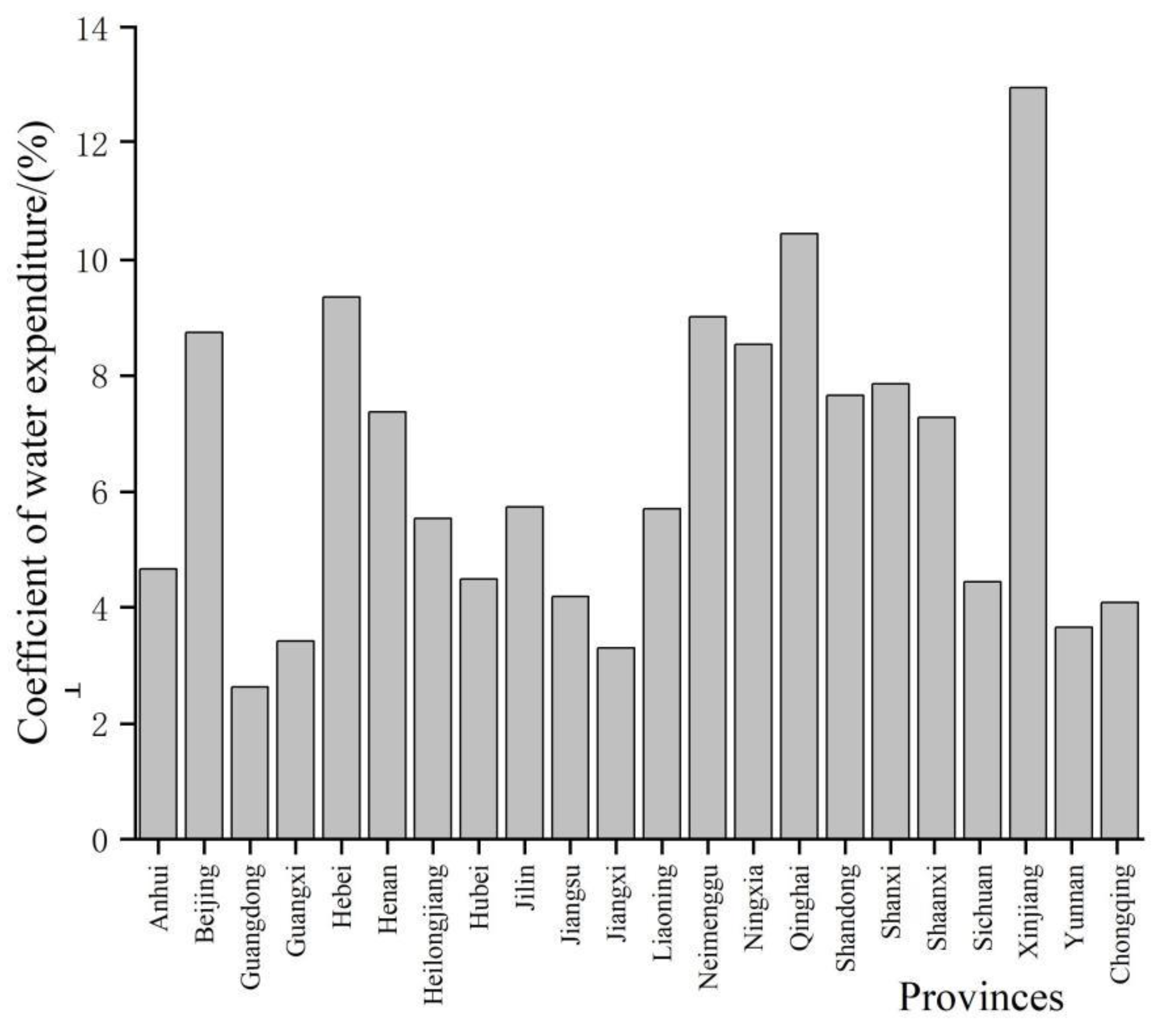
The WEC in each province was concentrated at 2.62–12.95% (Figure 1), with the highest value of 12.95% in the Xinjiang Uygur Autonomous Region, followed by Qinghai Province with 10.44%, and with the lowest value of 2.62% in Guangdong Province. The higher WEC values were concentrated in north China and northwest China, while the lower values were concentrated in south China and central China, reflecting the impact of water resources on WEC. The highest WEC was 5.95% in the Xinjiang Uygur Autonomous Region, and the lowest was 0.49% in Chongqing Province.

3.3.4. AWPA

The AWPA was between 617.300 yuan/hm² (89.555 $/hm²) and 2121.207 yuan/hm² (307.733 $/hm²;

Table 14. AWPA.

Province	Output p /yuan·hm−2	Precipitation r /mm	Water Consumption /m³·hm−2	AWPA /yuan·hm−2	AWPA /$·hm−2	AWPA /yuan·m−3	AWPA /$·m−3	Current Water Price /yuan·hm−2
Anhui	19,425.00	935.80	3750.00	904.336	131.196	0.241	0.0350	326.250
Beijing	14,085.00	506.00	2460.00	1229.488	178.368	0.500	0.0725	376.380
Guangdong	23,565.00	1993.60	11,130.00	617.300	89.555	0.055	0.0080	576.812
Guangxi	20,190.00	1602.70	11,805.00	687.851	99.790	0.058	0.0084	637.470
Hebei	14,085.00	442.70	2550.00	1316.210	190.949	0.516	0.0749	739.500
Henan	16,365.00	529.10	2355.00	1205.425	174.877	0.512	0.0743	706.500
Heilongjiang	18,585.00	728.30	6030.00	1026.765	148.958	0.170	0.0247	331.650
Hubei	20,715.00	893.50	5145.00	927.115	134.501	0.180	0.0261	318.990
Jilin	18,585.00	679.30	5160.00	1063.893	154.344	0.206	0.0299	232.200
Jiangsu	23,565.00	798.50	5205.00	984.354	142.805	0.189	0.0274	484.521
Jiangxi	20,190.00	1710.00	7125.00	665.489	96.546	0.093	0.0135	399.000
Liaoning	18,585.00	687.20	9000.00	1057.638	153.437	0.118	0.0171	927.000
Inner Mongolia	18,585.00	279.50	4065.00	1673.380	242.765	0.412	0.0598	455.280
Ningxia	17,595.00	345.70	10,590.00	1499.813	217.585	0.142	0.0206	958.395
Qinghai	13,740.00	374.00	7170.00	1433.710	207.995	0.200	0.0290	891.231
Shandong	15,315.00	558.90	2535.00	1170.653	169.832	0.462	0.0670	726.282
Shanxi	16,545.00	458.10	2835.00	1297.626	188.253	0.458	0.0664	765.450
Shaanxi	13,740.00	759.40	4305.00	999.047	144.936	0.232	0.0337	559.650
Sichuan	20,220.00	953.20	5475.00	896.598	130.074	0.164	0.0238	459.900
Xinjiang	16,380.00	174.70	8295.00	2121.207	307.733	0.256	0.0371	895.860
Yunnan	23,985.00	1008.00	5730.00	874.380	126.850	0.153	0.0222	525.728
Chongqing	20,385.00	1106.80	4875.00	830.954	120.550	0.170	0.0247	453.375

). The two provinces of Xinjiang and Inner Mongolia had the highest AWPA, amounting to 2121.207 yuan/hm² (307.733 $/hm²) and 1673.380 yuan/hm² (242.765 $/hm²), respectively. The lowest AWPA was 617.300 yuan/hm² (89.555 $/hm²) in Guangdong and 687.851 yuan/hm² (99.790 $/hm²) in Jiangxi. The reason for this is that the WEC was negatively correlated with the amount of precipitation and the output value per unit area. Under the influence of geographical factors, the precipitation and output value per unit area were relatively low in these two provinces, which led to a high average WEC and a higher AWPA than other provinces. Similarly, the precipitation and the output value per unit area of Guangdong and Jiangxi provinces were relatively high, and the average WEC of water users was low; thus, their AWPA was low.

The highest AWPA values were 0.516 yuan/m³ (0.0749 $/m³) and 0.512 yuan/m³ (0.0743 $/m³) in Hebei and Henan provinces, respectively, and the lowest were 0.055 yuan/m³ and 0.058 yuan/m³ in Guangdong and Guangxi provinces, respectively. From the river basin perspective, Qinghai, Tibet, Sichuan, Yunnan, Chongqing, Hubei, Hunan, Jiangxi, Anhui, Jiangsu, etc., in the Yangtze River Basin could bear a water price in the range of 0.164–0.241 yuan/m³ (0.024–0.034 $/m³). As can be seen from Table 13, the current irrigation terminal water price level in the Yangtze River Basin is between 0.062 and 0.124 yuan/m³ (0.009–0.018 $/m³). This shows that there are possibilities for adjusting the water prices. In the Yellow River Basin of Gansu, Ningxia, Inner Mongolia, Shaanxi, Shanxi, Henan, and Shandong, the AWPA was 0.142–0.516 yuan/m³ (0.018–0.075 $/m³), with an average value of 0.345 yuan/m³ (0.05 $/m³). The current water price level is 0.09–0.300 yuan/m³ (0.013–0.131 $/m³), with an average value of 0.188 yuan/m³ (0.027 $/m³). The price of water is completely within the range of AWPA.

4. Discussion

In this section, we will discuss the following three aspects: the consistencies and differences compared to previous studies, the limitations of the methods used, and the policy implications.

4.1. Comparison of Results

(1) WEC and AWPA

The WEC was high in northwest regions, such as Xinjiang and Gansu, while it was the lowest in Guangdong and Jiangxi provinces, with the highest AWPA per unit area in Xinjiang and Inner Mongolia, and the lowest for Hubei. The WEC and AWPA of less developed regions and water-scarce regions were higher than for the developed and water-rich regions. This phenomenon is consistent with the findings of Du [32].

Previous studies [15,33,34] have reported that AWPA is closely related to crop income and expenditures. AWPA is generally calculated as the water price that makes up for 5–15% of the crop output value or 10–13% of net income. This method comprehensively takes into account precipitation, the output value per unit area, and other factors. It was calculated that the WEC of food crops in each region ranged from 2.62% to 12.95%, and for cash crops was about 5%. The obtained results are compared with the previous results in

Table 15. Comparison of results.

	Previous Results		Results of This Study
Area	WEC (%)	AWPA (yuan/m3)	WEC (%)	AWPA (yuan/m3)
Xinjiang	10	0.0742	12.9	0.26
Henan (people victory irrigation area)	8–10	-	7.4	0.51
Shanxi (Linfen)	15 (of net benefit)	0.44	7.8	0.46
Shanxi (Lvliang)	15 (of net benefit)	0.37	7.8	0.46

. The AWPA of Linfen and Luliang in Shanxi [10] has been reported as 0.44 yuan/m³ (0.064 $/m³) and 0.37 yuan/m³ (0.054 $/m³), respectively, which is close to the results of this study (0.46 yuan/m³). Regarding the WEC in Henan Province (i.e., the proportion of output value), the result of this study was 7.4%, which is slightly lower than the previous results of 8–10% reported in [35]. As for the WEC in Xinjiang, the result of this study was 12.9%, which is slightly higher than the result of 10% from a previous study. The bearing capacity of this study was 0.26 yuan/m³, which is three times higher than the value reported in a previous study [9].

Based on the above results, the WEC and AWPA obtained in this study differ slightly from those obtained in previous studies. On the one hand, the value of WEC in previous studies is subjective, and lacks a comprehensive consideration due to personal influence factors. On the other hand, with the rapid development of economy, scientific, and technological levels, the relevant data have undergone major changes, and there is a lack of recent results for comparison.

(2) Contribution of influencing factors

Many researchers believe that the psychological effect is the main factor that influences the behavior of water consumers. Since psychological factors are difficult to quantify, only precipitation and economic factors were considered in this study. The explanation rate of the model was 70.8%, of which precipitation factors accounted for 45.2% and economic factors accounted for 25.6%. However, this does not mean that the rate of contribution of psychological factors to the WEC is lower than that of precipitation. This is because there is a certain correlation among the distribution of water resources, economic development, and psychological factors. Thus, 29.4% can be understood as the influence of partial psychological factors and other factors on WEC. For example, Lan et al. [36] suggested that the willingness of people to pay is inversely proportional to local precipitation and positively proportional to their income. The additional quantification and analysis of the contribution rate of psychological factors is needed and will be determined in future research.

4.2. Limitations

Grey situation decision making is an important part of modern decision-making theory and methods. It is focused on resolving the incommensurability and contradictions between multiple objectives [37,38]. This study used the grey decision principle to comprehensively assess the fitting effect of each regression model, adopting an equal weight assignment method for each indicator by referring to relevant studies [39,40,41]. Finally, this study used a log-linear model to analyze the relationship among WEC, precipitation, and output value. However, the weight of evaluation indicators in this method has always been the focus of debate, as it has a strong subjectivity. There is still space for existing research on how to objectively assign weight and balance decision making [42,43,44].

This study made a systematic assessment of the AWPA in China, focusing on making up for the shortcomings of previous methods, such as high subjectivity and large errors. The method we used is simple and has a wide application range. Meanwhile, the limitations of this method cannot be ignored. For example, a large amount of data is needed for calculation and fitting, which is not suitable for areas with limited data availability. In addition, this study only selected typical crops to calculate the AWPA and WEC. The crop structure in the study is relatively simple, so it is necessary to conduct further reasonable research according to the actual situation of local crops.

4.3. Policy Implications

Agricultural water price affordability and water price reform are closely related to local resource endowment and economic development. In areas with serious water shortage, the water expenditure coefficient is high, and the agricultural water price reform is more active; however, the agricultural reform process will undoubtedly be limited by economic development [45]. Therefore, we put forward the following policy implications from the perspective of the AWPA or WEC of each region, combined with local economic conditions and resource endowments.

(1) There is space for price adjustment in all regions. Therefore, the reform of agricultural water price should be further strengthened, while appropriate investment should be made to some local underdeveloped regions, and subsidies should be given to areas with a large capital gap, so as to ensure people’s livelihood and properly handle the relationship between the reform of agricultural water price and the alleviation of agricultural burden and poverty alleviation.

(2) The reform of agricultural water price should be carried out by category. For example, south China is rich in water resources and economically developed, and its WEC is low, resulting in a lack of motivation for agricultural water price reform. Therefore, it is necessary to strengthen publicity and guidance, and correspondingly adopt evaluation and accountability mechanisms and incentive mechanisms. In central China, the WEC is low, and the reform of agricultural water price is slow. This is likely because local water resources are relatively rich and the economy is underdeveloped, resulting in a lack of urgency for water saving and more capital investment. Therefore, special investment policies and measures, such as a strengthening evaluation, can be implemented to promote the agricultural reform process.

5. Conclusions

Through the grey situation decision-making theory, we chose the log-linear model to analyze the relationship among WEC, precipitation, and output value. This study also improved the way the value of WEC was assigned, which solved the problems of strong subjectivity and the limited evaluation scope of previous studies. Finally, the AWPA in different regions was calculated. In addition, the LMG method was used to measure the relative importance of each influencing factor, and for the first time the contribution degree of precipitation and output value to the water expense coefficient was given. The main conclusions are as follows:

(1) The contribution rate of precipitation to WEC is 45.2%, while the contribution rate of the output value is 25.6%;

(2) Overall, the AWPA in China is clearly higher than the current water price, and there is enough space for price adjustment. The AWPA is between 0.06 yuan/m³ and 0.52 yuan/m³. The WEC in each province is concentrated between 2.620% and 12.950%, with the highest value of 12.950% in Xinjiang Province, and the lowest value of 2.620% in Guangdong Province. This reflects the impact of water resources and economic development on WEC and AWPA. The calculated results are consistent with the reality and the method is reasonable.

(3) The AWPA can fully cover the current irrigation water price (0.05–0.30 yuan/m³). The AWPA in the Yellow River Basin is higher than that in the Yangtze River Basin; however, the space for adjustment in the Yellow River Basin is slightly smaller than that in the Yangtze River Basin.

References

- Wang, L.; Simayi, Z.; Yang, S. Research on economic bearing capacity of farmers to agricultural irrigation water prices in the ebinur lake basin. Sustainability 2019, 11, 2155. [Google Scholar] [CrossRef] [Green Version]
- Latinopoulos, D. Multicriteria decision-making for efficient water and land resources allocation in irrigated agriculture. Environ. Dev. Sustain. 2009, 11, 329–343. [Google Scholar] [CrossRef]
- Johansson, R.C.; Tsur, Y.; Roe, T.L.; Doukkali, R.; Dinar, A. Pricing irrigation water: A review of theory and practice. Water Policy 2002, 4, 173–199. [Google Scholar] [CrossRef]
- Li, X.R. The formation mechanism of agricultural water price in foreign countries and its enlightenment to China. Water Resour. Dev. Manag. 2019, 11, 71–75. [Google Scholar] [CrossRef]
- Jiang, W.L. Research on agricultural water price carrying capacity. China Water Resour. 2003, 11, 41–43. [Google Scholar] [CrossRef]
- Wang, H.; Ruan, B.Q.; Shen, D.J. Theory and Practice of Water Price for Sustainable Development; Beijing Science Press: Beijing, China, 2003. [Google Scholar] [CrossRef]
- Tang, Z. Analysis on the bearing capacity of farmers to irrigation water price in Zhangye City. Yellow River 2010, 32, 86–88. [Google Scholar] [CrossRef]
- Liao, Y.S.; Bao, Z.Y.; Huang, Q.W. Irrigation price reform and farmers’ affordability. Water Resour. Dev. Res. 2004, 12, 29–34. [Google Scholar] [CrossRef]
- Nian, Z.L.; Wang, M.Y. Analysis of water price bearing capacity of agricultural water users in Xinjiang. Water Econ. 2010, 28, 42–44. [Google Scholar] [CrossRef]
- Zhao, Y.Y.; Luo, P.; Chu, G.H. Analysis of farmers’ affordability of irrigation water price in hilly and mountainous areas. China Rural Water Hydropower 2014, 11, 147–150. [Google Scholar] [CrossRef]
- Parween, F.; Kumari, P.; Singh, A. Irrigation water pricing policies and water resources management. Water Policy 2020, 23, 130–141. [Google Scholar] [CrossRef]
- Lou, Y.P. Thoughts on econometric model methods. Chin. E-Commer. 2013, 15, 1. [Google Scholar] [CrossRef]
- Yang, M.H.; Cao, L.H.; Zhao, D. Research on the dynamic multi-objective agricultural water price setting model. People’s Yellow River 2018, 40, 155–159. [Google Scholar] [CrossRef]
- Jiang, Y.J.; Jiang, S.X. On the reform of agricultural water price in Jiangxi province. Price Monthly 2014, 11, 1–6. [Google Scholar] [CrossRef]
- Chen, J.; Chu, L.L.; Chen, D. Research on farmers’ psychological affordability of irrigation water price based on CVM. Water Econ. 2008, 5, 39–41. [Google Scholar] [CrossRef]
- Mitchel, L.R.; Carson, R. Using Surveys to Value Public Goods: The Contingent Valuation Method; Resources for the Future: Washington, DC, USA, 1989. [Google Scholar] [CrossRef]
- Aydogdu, M.H.; Bilgic, A. An evaluation of farmers’ willingness to pay for efficient irrigation for sustainable usage of resources: The GAP-Harran plain case, Turkey. J. Integr. Environ. Sci. 2016, 13, 175–186. [Google Scholar] [CrossRef] [Green Version]
- Wu, M.Y.; Yang, K.; Liu, L. Evaluation of reclaimed water based on grey situation decision making and combination weighting method. J. Water Resour. Water Eng. 2018, 29, 111–117. [Google Scholar] [CrossRef]
- Liu, S.F.; Lin, Y. Grey information: Theory and practical applications. Kybernetes 2006, 34, 89–92. [Google Scholar] [CrossRef]
- Jiang, S.Q. Research on Grey Relational Decision Model Based on General Grey Number and Its Application. Ph.D. Thesis, Nanjing University of Aeronautics and Astronautics, Nanjing, China, 2018. [Google Scholar]
- Guo, Y.; Liu, P.F. Damage assessment of airfield target based on grey relational analytic hierarchy process. Sichuan Ordnance J. 2014, 8, 55–58. [Google Scholar] [CrossRef]
- Wu, Y.; Li, W.; Ma, D.Z. Comprehensive evaluation of different maize varieties by DTOPSIS method based on entropy weighting. J. Maize Sci. 2019, 27, 32–41. [Google Scholar] [CrossRef]
- Wang, H.S.; Guo, C.F.; Tian, Y.G. Application of weighted grey situation decision in ship-aircraft cooperative submarine search. Ordnance Ind. Autom. 2015, 34, 33–35. [Google Scholar] [CrossRef]
- Grömping, U. Relative importance for linear regression in R: The package relaimpo. J. Stat. Softw. 2006, 76, 925–933. [Google Scholar] [CrossRef]
- Long, G.; Cao, X. Grey situation decision method comprehensive evaluation of potato varieties (or lines). J. Anhui Agric. Sci. 2009, 37, 11925–11927. [Google Scholar] [CrossRef]
- Zhang, Z.; Wang, L. Advanced Statistics Using R; ISDSA Press: Granger, IN, USA, 2017. [Google Scholar]
- Li, H.W.; Wu, Y.P.; Liu, S.G. Regional contributions to interannual variability of net primary production and climatic attributions. Agric. For. Meteorol. 2021, 303, 108384. [Google Scholar] [CrossRef]
- Ding, Y.B.; Gong, X.L. Attribution of meteorological, hydrological and agricultural drought propagation in different climatic regions of China. Agric. Water Manag. 2021, 255, 106996. [Google Scholar] [CrossRef]
- Shi, P.J.; Chen, Y.Q.; Ma, H. Contribution rate of relative oxygen content in near-surface atmosphere over the Tibetan Plateau. Chin. Sci. Bull. 2021, 64, 715–724. [Google Scholar] [CrossRef] [Green Version]
- Zhang, N. Research on Grey Situation Group Decision Model and Its Application. Ph.D. Thesis, Nanjing University of Aeronautics and Astronautics, Nanjing, China, 2016. [Google Scholar]
- Chen, D. Study on Irrigation Water Price and Farmers’ Affordability in Seasonal Water Shortage Irrigated Areas in Southern China. Ph.D. Thesis, Hohai University, Nanjing, China, 2007. [Google Scholar]
- Du, L.J.; Liu, C.S. Preliminary study on the calculation of farmers’ irrigation water cost bearing capacity. Water Resour. Hydropower Technol. 2011, 42, 59–62. [Google Scholar] [CrossRef]
- Guo, Q.L.; Feng, Q.; Yang, Y.S. Research on water price of sustainable development in the middle reaches of Heihe River. Yellow River 2007, 29, 65–66. [Google Scholar] [CrossRef]
- Zheng, T.H.; Zhang, C. Agricultural Water Price Comprehensive Reform Pilot Training Handout; China Water and Hydropower Press: Beijing, China, 2008. [Google Scholar]
- Zhuo, H.W.; Wang, W.M.; Song, S. Research on farmers’ ability to bear agricultural water price. China Rural Water Hydropower 2005, 11, 1–5. [Google Scholar] [CrossRef]
- Lan, M.; Wang, C.C. Assessing the impact of water price reform on farmers’ willingness to pay for agricultural water in northwest China. J. Clean. Prod. 2019, 234, 1072–1081. [Google Scholar] [CrossRef]
- Zeng, L.; Zhang, C.Z.; Lu, S.S. Application of grey situation decision in evaluation of new rice varieties. J. Anhui Agric. Sci. 2013, 41, 1466–1468. [Google Scholar] [CrossRef]
- Wang, H.H.; Zhu, J.J.; Fang, Z.G. Information aggregation method for multi-stage linguistic evaluation based on grey relational degree. Control Decis. 2013, 28, 109–114. [Google Scholar] [CrossRef]
- Wu, X.Z.; Ruan, P.J.; Pan, G.Y. Application of grey situation decision in comprehensive evaluation of maize varieties. J. Mt. Agric. Biol. 2001, 20, 407–411. [Google Scholar] [CrossRef]
- Li, W.Y.; Wei, Y.; Kong, F.N. Application of DTOPSIS method in comprehensive evaluation of strawberry varieties. Chin. J. Plant Physiol. 2018, 54, 925–930. [Google Scholar] [CrossRef]
- Deng, J.L. Grey Prediction and Decision; Huazhong University of Science and Technology Press: Wuhan, China, 2002. [Google Scholar]
- Zhu, J.J.; Liu, S.F. Aggregation method for multi-stage multivariate judgment preference in group decision making. Control Decis. 2008, 23, 730–734. [Google Scholar] [CrossRef]
- Xu, Z.S. A method based on the dynamic weighted geometric aggregation operator for dynamic hybrid multi-attribute group decision making. Int. J. Uncertain. Fuzziness Knowl. Based Syst. 2009, 17, 15–33. [Google Scholar] [CrossRef]
- Qi, J.S.; Xia, L.K.; Huang, B. Application of DTOPSIS method and grey situation decision method based on entropy weight in maize varieties regional experiment. Crops 2021, 1, 60–67. [Google Scholar] [CrossRef]
- Jiang, W.L.; Feng, X.; Liu, Y. Analysis of regional differences in comprehensive reform of agricultural water price in China. Prog. Sci. Technol. Water Resour. Hydropower 2020, 40, 1–5. [Google Scholar] [CrossRef]