
Simultaneous Estimation of a Contaminant Source and Hydraulic Conductivity Field by Combining an Iterative Ensemble Smoother and Sequential Gaussian Simulation

Abstract
:1. Introduction
2. Problem Formulation
3. Methodology
- Step 1
- Set iteration counter i = 1.
- Step 2
- Generate input ensemble from the prior distribution.
- (a)
- Based on directly measured hydraulic conductivities (hard data) generated Ne realizations of hydraulic conductivity field; the hydraulic conductivity value at pilot points was obtained from Ne realizations of the hydraulic conductivity field.
- (b)
- An initial ensemble of contaminant source parameters was generated by sampling from priori distribution of contaminant source parameters (the location and strength of contaminant source for each stress period).
- Step 3
- Generate output ensemble by evaluating the forward model.
- Step 4
- Obtain the update ensemble using ILUES algorithm.
- Step 5
- Set i = i + 1. If , stop; otherwise, let , go to Step 3.
4. Illustrative Example
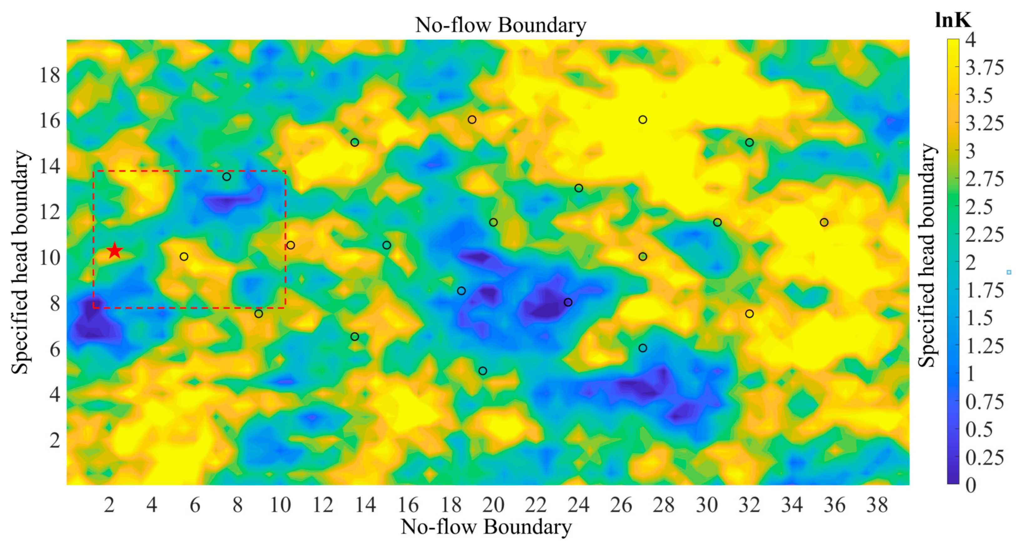
4.1. Problem Description
4.2. Assessment Criteria
5. Results and Discussions
5.1. Scenario 1
5.2. Scenario 2
5.3. Scenario 3
5.4. Scenario 4
6. Conclusions
- In this study, the iterative local updating ensemble smoother (ILUES) and sequential gaussian simulation (SGSIM) in geostatistics were combined to realize the simultaneous inversion of contaminant sources and hydraulic conductivity field. As an efficient data assimilation method, the ILUES algorithm was adopted to construct the framework for solving groundwater inverse problems. Specifically, the inversion of hydraulic conductivities was converted to the estimation of hydraulic conductivity at pilot points;
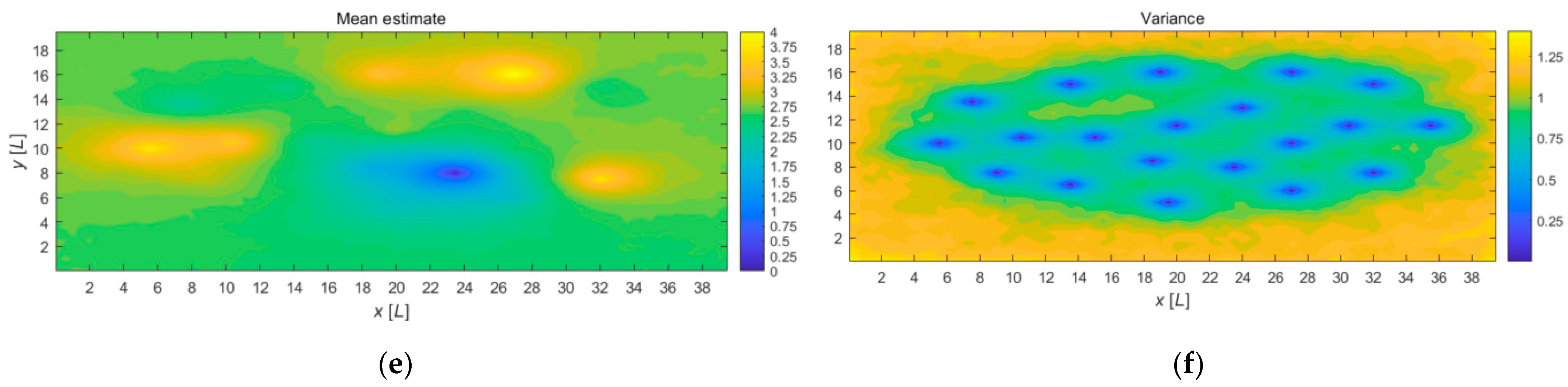
- With the increasing ensemble size, our proposed method can obtain more accurate estimation of both source characteristics and the hydraulic conductivity field. Furthermore, too large an ensemble size may result in heavy computational burden, and the sensitivity of estimation results to the ensemble size becomes weak. For this study, the ensemble size of 2000 is sufficient to provide satisfactory results;
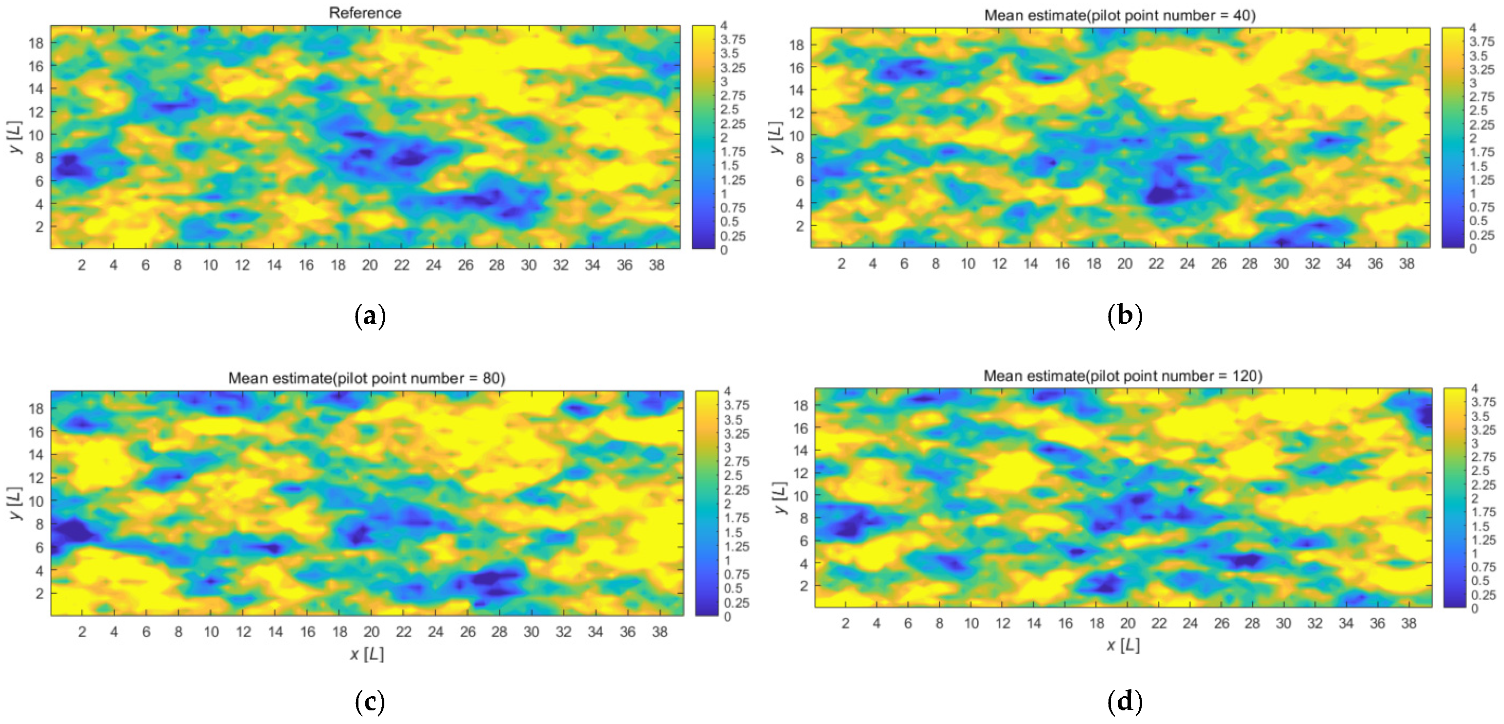
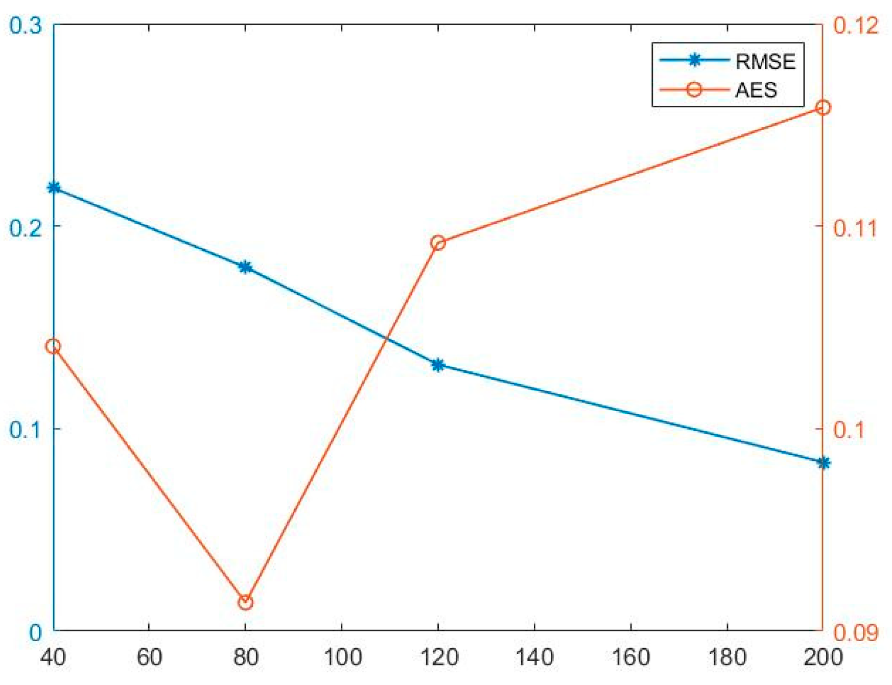
- With the increasing number of pilot points, the RMSE metric decreases monotonically, but the AES metric characterizing the uncertainty or confidence of the estimation tends to first decrease and then increase. Perhaps it can be explained that the elevated number of pilot point introduce noises while bringing more additional information. For this study, the pilot point number of 80 might be a reasonable choice for this study;
- The temporal distribution of measurements influences the identification of contaminant source parameter and hydraulic conductivities. To some extent, the proposed method performs better with the increase in the observations. Specially, the propose method performs better with the increase in the overlapping degree of monitoring time and pollution occurrence. For this study, the inversion results by assimilating the hydraulic head and contaminant concentration data collected every 4 days clearly outperforms that by assimilating the data collected in the last 10 days.
Author Contributions
Funding
Data Availability Statement
Conflicts of Interest
References
- Lee, S.; Carle, S.F.; Fogg, G.E. Geologic heterogeneity and a comparison of two geostatistical models: Sequential Gaussian and transition probability-based geostatistical simulation. Adv. Water Resour. 2007, 30, 1914–1932. [Google Scholar] [CrossRef]
- Bailey, R.T.; Baù, D. Estimating geostatistical parameters and spatially-variable hydraulic conductivity within a catchment system using an ensemble smoother. Hydrol. Earth Syst. Sci. 2012, 16, 287–304. [Google Scholar] [CrossRef] [Green Version]
- Cao, Z.; Li, L.; Chen, K. Bridging iterative Ensemble Smoother and multiple-point geostatistics for better flow and transport modeling. J. Hydrol. 2018, 565, 411–421. [Google Scholar] [CrossRef]
- Bailey, R.; Baù, D. Ensemble smoother assimilation of hydraulic head and return flow data to estimate hydraulic conductivity distribution. Water Resour. Res. 2010, 46. [Google Scholar] [CrossRef]
- Erdal, D.; Cirpka, O.A. Joint inference of groundwater–recharge and hydraulic–conductivity fields from head data using the ensemble Kalman filter. Hydrol. Earth Syst. Sci. 2016, 20, 555–569. [Google Scholar] [CrossRef] [Green Version]
- Zhang, J.; Lin, G.; Li, W.; Wu, L.; Zeng, L. An Iterative Local Updating Ensemble Smoother for Estimation and Uncertainty Assessment of Hydrologic Model Parameters with Multimodal Distributions. Water Resour. Res. 2018, 54, 1716–1733. [Google Scholar] [CrossRef]
- Zhou, H.; Gómez-Hernández, J.; Li, L. Inverse methods in hydrogeology: Evolution and recent trends. Adv. Water Resour. 2014, 63, 22–37. [Google Scholar] [CrossRef] [Green Version]
- Evensen, G. The Ensemble Kalman Filter: Theoretical formulation and practical implementation. Ocean Dynam. 2003, 53, 343–367. [Google Scholar] [CrossRef]
- Franssen, H.J.H.; Kinzelbach, W. Ensemble Kalman filtering versus sequential self-calibration for inverse modelling of dynamic groundwater flow systems. J. Hydrol. 2009, 365, 261–274. [Google Scholar] [CrossRef]
- Houtekamer, P.L.; Zhang, F. Review of the Ensemble Kalman Filter for Atmospheric Data Assimilation. Mon. Weather Rev. 2016, 144, 4489–4532. [Google Scholar] [CrossRef]
- Leeuwen, P.; Evensen, G. Data assimilation and inverse methods in terms of a probabilistic formulation. Mon. Weather Rev. 1996, 124, 2898–2913. [Google Scholar] [CrossRef]
- Ju, L.; Zhang, J.; Meng, L.; Wu, L.; Zeng, L. An adaptive Gaussian process-based iterative ensemble smoother for data assimilation. Adv. Water Resour. 2018, 115, 125–135. [Google Scholar] [CrossRef]
- Li, L.; Stetler, L.; Cao, Z.; Davis, A. An iterative normal-score ensemble smoother for dealing with non-Gaussianity in data assimilation. J. Hydrol. 2018, 567, 759–766. [Google Scholar] [CrossRef]
- RamaRao, B.S.; LaVenue, A.M.; Marsily, G.D.; Marietta, M.G. Pilot Point Methodology for Automated Calibration of an Ensemble of conditionally Simulated Transmissivity Fields: 1. Theory and Computational Experiments. Water Resour. Res. 1995, 31, 475–493. [Google Scholar] [CrossRef]
- Harbaugh, A.W.; Banta, E.R.; Hill, M.C.; McDonald, M.G. MODFLOW-2000, The U.S. Geological Survey Modular Ground-Water Model—User Guide to Modularization Concepts and the Ground-Water Flow Process; Open-File Report; U.S. Geological Survey: Reston, VI, USA, 2000. [Google Scholar]
- Zheng, C.; Wang, P.P. MT3DMS: A Modular Three-Dimensional Multispecies Transport Model for Simulation of Advection, Dispersion, and Chemical Reactions of Contaminants in Groundwater Systems; Documentation and User’s Guide; Engineer Research and Development Center: Vicksburg, MS, USA, 1999. [Google Scholar]
- Alcolea, A.; Carrera, J.; Medina, A. Pilot points method incorporating prior information for solving the groundwater flow inverse problem. Adv. Water Resour. 2006, 29, 1678–1689. [Google Scholar] [CrossRef]
- Deutsch, C.V.; Journel, A.G. GSLIB:* Geostatistical Software Library and Users Guide; Oxford University Press: Oxford, UK, 1998. [Google Scholar]


| Parameter | Units | Value |
|---|---|---|
| Grid size | m × m | 0.5 × 0.5 |
| Aquifer thickness | m | 1.0 |
| Effective porosity | none | 0.30 |
| Longitudinal dispersivity | m | 2.0 |
| Transverse dispersivity | m | 0.6 |
| Simulation time | day | 40 |
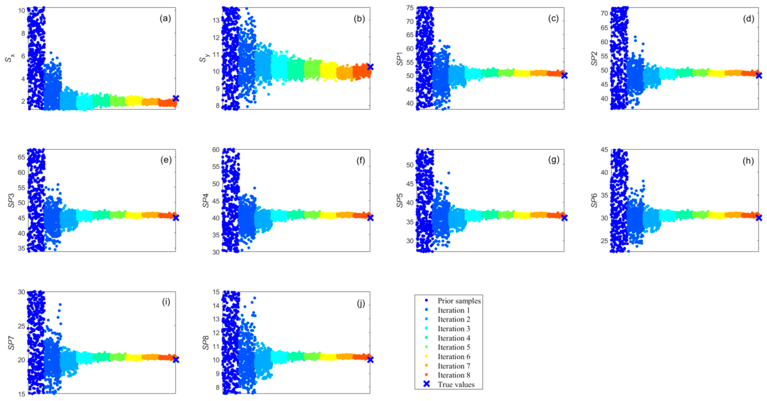
| Contaminant Parameter | Prior Range | Actual Value |
|---|---|---|
| Sx (m) | [1.25–10.25] | 2.25 |
| Sy (m) | [7.75–13.75] | 10.25 |
| (kg/d) | [35–75] | 50 |
| (kg/d) | [35–75] | 48 |
| (kg/d) | [30–70] | 45 |
| (kg/d) | [30–60] | 40 |
| (kg/d) | [25–55] | 36 |
| (kg/d) | [22–45] | 30 |
| (kg/d) | [15–30] | 20 |
| (kg/d) | [7–15] | 10 |
| Scenario No. | Case No. | Conditioned K | Conditioned h+C | Number of pp (Np) | Method | Ensemble Size |
|---|---|---|---|---|---|---|
| Scenario 1 | Case 1 | 20 | − | − | SGSIM | − |
| Scenario 2 | Case 2.1 | 20 | 220 | 80 | SGSIM-ILUES | 500 |
| Case 2.2 | 20 | 220 | 80 | SGSIM-ILUES | 1000 | |
| Case 2.3 | 20 | 220 | 80 | SGSIM-ILUES | 2000 | |
| Scenario 3 | Case 2.3 | 20 | 220 | 80 | SGSIM-ILUES | 2000 |
| Case 3.1 | 20 | 220 | 40 | SGSIM-ILUES | 2000 | |
| Case 3.2 | 20 | 220 | 120 | SGSIM-ILUES | 2000 | |
| Scenario 4 | Case 2.3 | 20 | 220 | 80 | SGSIM-ILUES | 2000 |
| Case 4.1 | 20 | 220 * | 80 | SGSIM-ILUES | 2000 | |
| Case 4.2 | 20 | 120 | 80 | SGSIM-ILUES | 2000 |
Publisher’s Note: MDPI stays neutral with regard to jurisdictional claims in published maps and institutional affiliations. |
© 2022 by the authors. Licensee MDPI, Basel, Switzerland. This article is an open access article distributed under the terms and conditions of the Creative Commons Attribution (CC BY) license (https://creativecommons.org/licenses/by/4.0/).
Share and Cite
Jiang, S.; Zhang, R.; Liu, J.; Xia, X.; Li, X.; Zheng, M. Simultaneous Estimation of a Contaminant Source and Hydraulic Conductivity Field by Combining an Iterative Ensemble Smoother and Sequential Gaussian Simulation. Water 2022, 14, 757. https://doi.org/10.3390/w14050757
Jiang S, Zhang R, Liu J, Xia X, Li X, Zheng M. Simultaneous Estimation of a Contaminant Source and Hydraulic Conductivity Field by Combining an Iterative Ensemble Smoother and Sequential Gaussian Simulation. Water. 2022; 14(5):757. https://doi.org/10.3390/w14050757
Chicago/Turabian StyleJiang, Simin, Ruicheng Zhang, Jinbing Liu, Xuemin Xia, Xianwen Li, and Maohui Zheng. 2022. "Simultaneous Estimation of a Contaminant Source and Hydraulic Conductivity Field by Combining an Iterative Ensemble Smoother and Sequential Gaussian Simulation" Water 14, no. 5: 757. https://doi.org/10.3390/w14050757