
Assessing the Performance of LISFLOOD-FP and SWMM for a Small Watershed with Scarce Data Availability


1
IKT-Institute for Underground Infrastructure, Exterbruch, 45886 Gelsenkirchen, Germany
2
Department of Urban Water Management, Hydrology and Hydraulic Engineering, Faculty of Civil Engineering, Campus Mülheim, University of Applied Sciences Ruhr West, Duisburger Str. 100, 45479 Mülheim an der Ruhr, Germany
3
Department of Urban Water Management and Environmental Engineering, School for Infrastructure and Environment, Faculty of Civil and Environmental Engineering, Ruhr-Universität Bochum, Universitätsstraße 150, 44801 Bochum, Germany
4
School of Energy, Construction and Environment & Centre for Agroecology, Water and Resilience, Coventry University, Coventry CV1 5FB, UK
*
Authors to whom correspondence should be addressed.
Water 2022, 14(5), 748; https://doi.org/10.3390/w14050748
Submission received: 28 January 2022
/
Revised: 22 February 2022
/
Accepted: 23 February 2022
/
Published: 26 February 2022
(This article belongs to the Special Issue Urban and River Flooding: Theory, Experimental and Numerical Models, and Applications in Hydraulic Engineering)
Abstract
:Flooding events are becoming more frequent and the negative impacts that they are causing globally are very significant. Current predictions have confirmed that conditions linked with future climate scenarios are worsening; therefore, there is a strong need to improve flood risk modeling and to develop innovative approaches to tackle this issue. However, the numerical tools available nowadays (commercial and freeware) need essential data for calibration and validation purposes and, regrettably, this cannot always be provided in every country for dissimilar reasons. This work aims to examine the quality and capabilities of open-source numerical flood modeling tools and their data preparation process in situations where calibration datasets may be of poor quality or not available at all. For this purpose, EPA’s Storm Water Management Model (SWMM) was selected to investigate 1D modeling and LISFLOOD-FP was chosen for 2D modeling. The simulation results obtained with freeware products showed that both models are reasonably capable of detecting flood features such as critical points, flooding extent, and water depth. However, although working with them is more challenging than working with commercial products, the quality of the results relative to the reference map was acceptable. Therefore, this study demonstrated that LISFLOOD-FP and SWMM can cope with the lack of these variables as a starting point and has provided steps to undertake to generate reliable results for the need required, which is the estimation of the impacts of flooding events and the likelihood of their occurrence.
Keywords:
urban flood; numerical modeling; SWMM; LISFLOOD-FP; hydrodynamics; stormwater; microscale modeling1. Introduction
In recent years, the number of floods occurring in urban environments has increased significantly [1,2]. Urban floods generally happen as a combination of meteorological and hydrological extremes, such as extreme rain events, and are characterized by high-intensity flows combined with short response times, leading to severe losses [3,4]. The flooding consequences can be tangible or intangible—for example, immediate death, injury, contaminated water harms, possession losses, damaged homes, financial worries, forced move, and fear of vacant homes being burgled [5]. In addition to climate change, rapid land development, coupled with inadequate and aging infrastructure, likely leads to frequent urban flooding in the future [6]. According to recent “flood list news” [7], severe events have caused flooding in Developing Countries (DCs) such as Afghanistan, Ethiopia, Iran, Kenya, and Somalia. However, even developed countries are not free from these events: in August 2021, flooding caused the death of at least 22 people in Tennessee, USA [8]; in July 2021, flooding after heavy rain caused more than 180 fatalities in Germany [9].
Among the methodologies employed to prevent or mitigate flood losses, hydrodynamic modeling has shown promising results [10,11,12,13]. Such models are numerical models based on fundamental equations of hydrodynamics that aim to simulate the rainfall runoff and its following inundation processes [14]. Hydrodynamic models can be classified based on their dimensionality as “0D”, “1D”, “2D”, “3D”, and combinations of them. To date, the models predominantly used in urban flood modeling are 1D, 2D, and coupled 1D/2D models [15,16].
One-dimensional models are mainly employed when a highly “detailed resolution” is not required, for rapid analysis or in the case of having a “dominant flow direction” [17,18]. These models regularly use the 1D representations of the Saint-Venant Equations (SVEs). In urban flood modeling, they are predominantly used to simulate the sewerage system flows. The only outcome of the 1D sewer network modeling is the floodwater volume at each maintenance hole or drainage inlet, while other flooding features are unclear [19].
Two-dimensional models provide details of the water-flow propagation without considering the sewerage system, usually by relying on 2D SVEs [19]. They discretize the surface into a continuous hydraulic cell mesh and the size of these cells influences the accuracy of results and the computation time [20]. The simulation results present the inundation extent and the flow dynamics, in particular velocities and depths. Since the model does not account for sewerage networks, the flood risk can be underestimated or overestimated [18].
The dual drainage method was introduced due to the need for an approach capable of reflecting the interaction between the surface and the sewerage network bidirectionally. A 1D/2D model of an urban system represents the sewerage system in one dimension and the surface in two dimensions, with flow exchanges happening through maintenance holes or drainage inlets [21,22,23]. This kind of model can predict water levels and flow velocities in two-directional components, and overflow volumes, so it comes the closest to real conditions [18].
Hydrodynamic modeling is a popular choice because of economic motivations and the amount of information it provides; however, it cannot replace experimental techniques. Instead, they complete each other. Experimental evidence is needed to confirm the modeling results [24]. Although progress has been made in dataset productions to calibrate and validate hydrodynamic models, a lack of information still exists. In some areas, there is no access to flow data recording equipment, and in areas where these are available, the expenses of maintaining and optimizing such devices and regularly controlling them can make the collecting calibration data infeasible or unreliable [25]. In particular, in DCs, obtaining detailed hydrological and hydraulic data is challenging; consequently, approaches that do not demand detailed data for generating acceptable results are of interest [26]. The lack of resources in urban flood modeling is not limited to hydraulic and hydrological calibration data, but also many do not have access to advanced commercial software products [4]. Furthermore, the smaller the watershed considered, the greater the problems in accurately modeling its characteristics. High levels of heterogeneity typically characterize small watersheds (geological and hydrological); thus, flow pathways may be sensitive to prevailing local climactic conditions and primary physical watershed characteristics. Within this field, the hydrological watershed pathways are delineated into surface flow (runoff) and subsurface flow, with subsurface flow comprising lateral soil water flow (interflow) and groundwater flow (baseflow). Flood risk assessments are primarily undertaken at the macroscale or mesoscale; however, a microscale modeling is needed for a detailed assessment of crucial elements. Microscale modeling aims to conduct hazard and risk assessments at the scale of individual facilities or buildings, which is feasible thanks to recent advances in flood simulation, making modeling with up to 10 cm data resolution possible. In such analyses, flood hazard assessment relies on detailed spatial models to solve the 2D SVEs. In general, there are three methods to present the impact of buildings on the surface runoff movements in flood modeling; the first method shows the effect of buildings using porosity parameters, which allows low-resolution data to be used and reduces modeling time, but it is not recommended for microscale modeling. In the second method, called building block, a building is represented by increasing the height of the DEM cells to the height of the roof of the building. In the third method, called building hole, the area in which a building is located is not considered in modeling, and instead, a hole with closed-boundary conditions is created in the model. One of the purposes of microscale modeling is the evaluation of the flood protection measures and their efficacy. This approach can provide an acceptable illustration of small topographic variations and small-scale structural elements. This simulation approach allows the user to accurately represent the surface components, buildings details, and changes in terrain elevation and define a specific roughness coefficient for each surface element. This method’s advantage is that the roughness coefficient calibrations become critical [27,28].
To address the gap highlighted, this paper aims at assessing the performance of two existing numerical tools, LISFLOOD-FP and SWMM, in a small watershed with scarce data. Their outcomes were combined with observations made in the field and simulations were made at the scale of a building (microscale) [27], aiming to assess urban flood modeling at different scales while facing resource paucity and providing some suggestions for future approaches within similar situations. Thus, the approaches developed in this study could be extremely useful for countries or municipalities in which data availability is scarce.
2. Methodology
2.1. Case Study
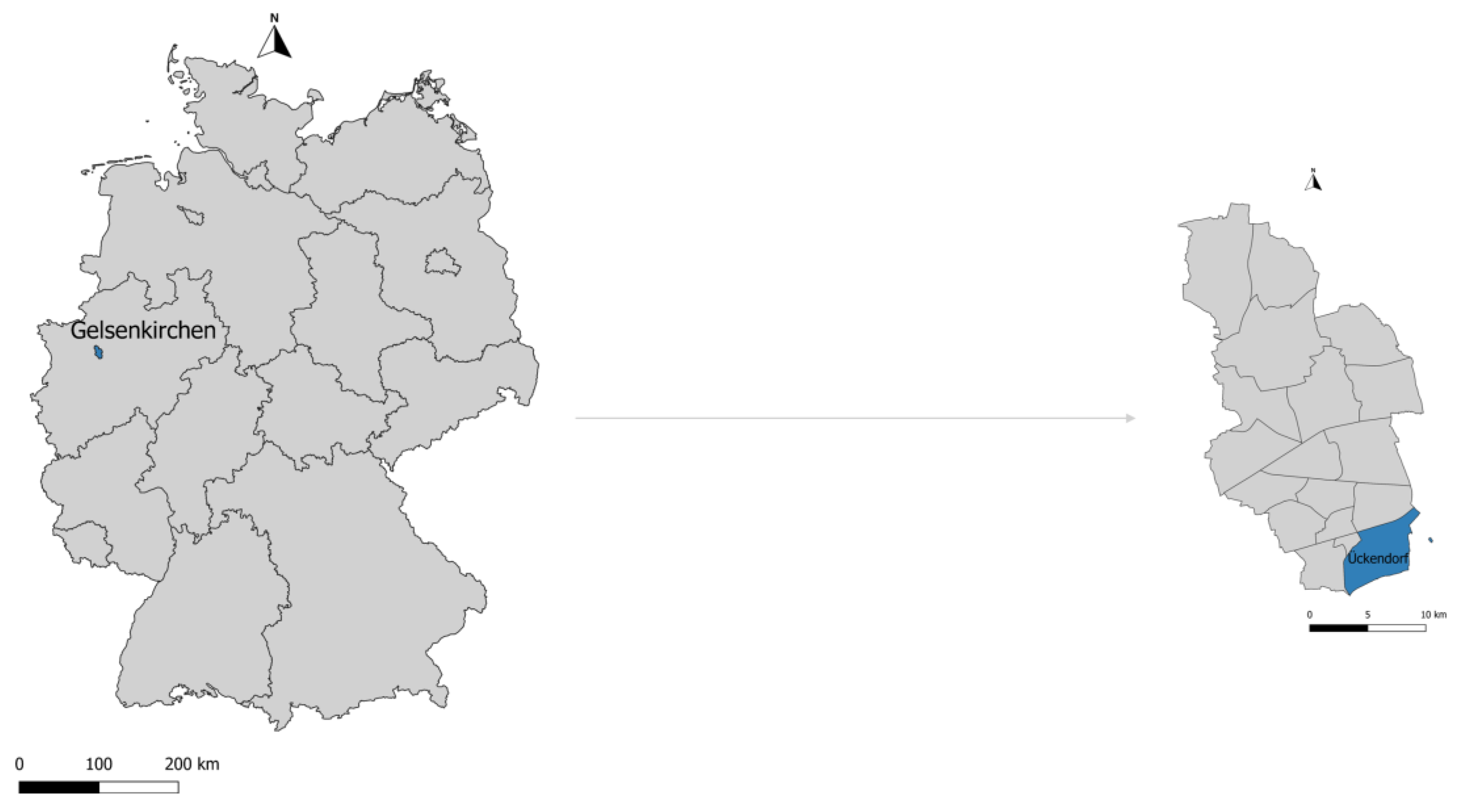
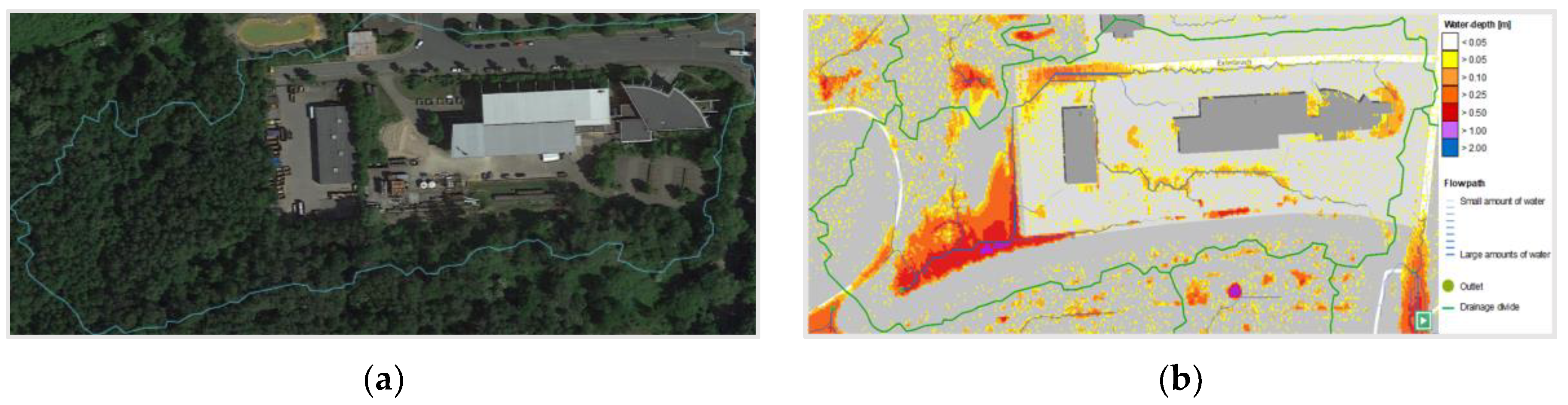
A single watershed located Southeast of Gelsenkirchen, Germany, in a region called Ueckendorf (Figure 1), has been investigated in this work (Figure 2a). The selected watershed of 3.98 hectares lies between latitudes 51°30′29.9772″ N and 51°30′35.6904″ N and longitudes 7°07′52.255″ E and 7°08′11.526″ E, with an average altitude of 54.57 m above mean sea level. It receives around 813 mm of annual rainfall, and its temperature range varies from −9.1 °C to 40.0 °C, based on the most recent statistics [29]. Apart from the official flood hazard map [30], no details of previous floods in the area were available (Figure 2b); therefore, this has been identified as the most suitable case to represent the lack of datasets needed for calibration and validation.
To assess the potential of the freeware products within data scarcity for the site selected, the official flood hazard map produced for a 2D rainfall-runoff simulation for a 100-year rain event was selected as the reference.
2.2. Numerical Models Adopted
SWMM and LISFLOOD-FP are both robust models identified in the literature for modeling urban floods as freeware products [34]; therefore, they have been selected for this study as freeware alternatives, especially considering the financial limitations that many countries or operators may have on top of data scarcity. Their performance and reliability in the case of scarce data availability have been assessed.
2.2.1. SWMM
The SWMM developed by the USA’s environmental protection agency, commonly referred to as SWMM, was first introduced in 1971. SWMM is broadly considered as an efficient 1D sewerage system model. For runoff quantity and quality simulation, SWMM employs 1D SVEs:
where x is distance, t is time, A is flow cross-section area, Q is flow rate, H is hydraulic head of water in the conduit (Z + Y), Z is conduit invert elevation, Y is conduit water depth, Sf is friction slope, and g is the gravitational acceleration.
SWMM is incapable of simulating surface runoff and only provides users with a conceptual representation of the surface by discretizing the study area into smaller hydrological units called subcatchments and predicts the rainfall-runoff process of each of them without the ability of surface routing.
2.2.2. LISFLOOD-FP
Originally, Bates and De Roo [35] developed the 2D raster-based hydraulic model LISFLOOD-FP. This model simulates a shallow-water wave using an explicit finite difference scheme. LISFLOOD-FP solves two equations to handle the continuity of momentum between cells and continuity of mass in each cell. In fact, the 1D momentum equation is solved for each face of each grid cell (Equation (2)). The continuity equation for each cell is:
where Δt is time step, Q is the flow between cells, h is the water depth at each cell center, A is the water surface or cell area, and i and j are spatial indices in x and y directions, respectively [36]. The following equation describes the momentum equation to calculate the flow between two cells:
where Δx is the cell width, g is gravitational acceleration, qt is flow from the previous time step Qt divided by cell width Δx, S is the water surface slope between cells, n is Manning’s roughness coefficient, and hflow is the depth between cells through which water can flow, defined by the water depths and cell elevations.
LISFLOOD-FP can demonstrate flooding development and produce a maximum flood extent estimation. The model accounts for spatially uniform precipitation, infiltration, and evaporation and does not allow for a flexible cell size, so it uses a uniform mesh throughout the domain and uses DEM cells as the mesh to represent the floodplain [35,37]. This model provides users with different solvers to simulate the flood wave propagation. In the current paper, two of the solvers offered by LISFLOOD-FP were used [4,38]:
- The “acceleration” solver neglects the convective acceleration term;
- The “Roe” solver solves the full shallow-water equations. Despite being the most comprehensive solver, it has been reviewed only for a limited number of scenarios.
2.3. Data Collection and Manipulation
Several variables have been considered when building both models. Table 1 gives an overview of sources from which the data were collected.
Due to the unavailability of the necessary information to calibrate the model, great care was spent preparing the input datasets which were gathered from reliable sources (Table 1), and were then validated by numerous site surveys and observations as well as taking advantage of Geographic Information System (GIS) tools such as QGIS software and Google Maps, which are freely available.
The primary data for building the SWMM model was sewerage system dimensions and locations. Dimensions were extracted from a CAD map and augmented and validated by onsite data investigation; both the CAD map and the measurement tool used in onsite data investigation have an accuracy of ±0.005 m. The sewerage system model was then characterized by losses and Manning’s coefficient of the conduits [40]. The location of sewerage system elements was validated by overlaying the CAD map on the watershed DEM with a vertical accuracy of ±0.2 m and no horizontal inaccuracy [44], using QGIS. The raw LiDAR data with a vertical accuracy of ±0.15 m and a horizontal accuracy of ±0.3 [43] were used to build the subcatchments, which were then individually characterized by depression storage depths [40], Manning’s coefficient [40], infiltration parameters [40] and the impervious ratio [40]. The watershed includes rooftops, driveways, vegetation, and forests. The dominant soil type of the watershed surface layer is loess, which is a clastic predominantly silt-sized sediment, over deep to very deep boulder clay [42,46]; in the hydrologic soil classification offered by the natural resource conservation, loess is assigned to group B; information of soil characteristics was used to estimate infiltration parameters. The classical Horton method was selected to take the infiltration losses into account; this method is the most suitable for heavy storms. It must be noted that SWMM does not calculate infiltration losses for impervious areas [40]. Table 2 shows the selected depression storage depths, the selected surface Manning n values and infiltration parameters.
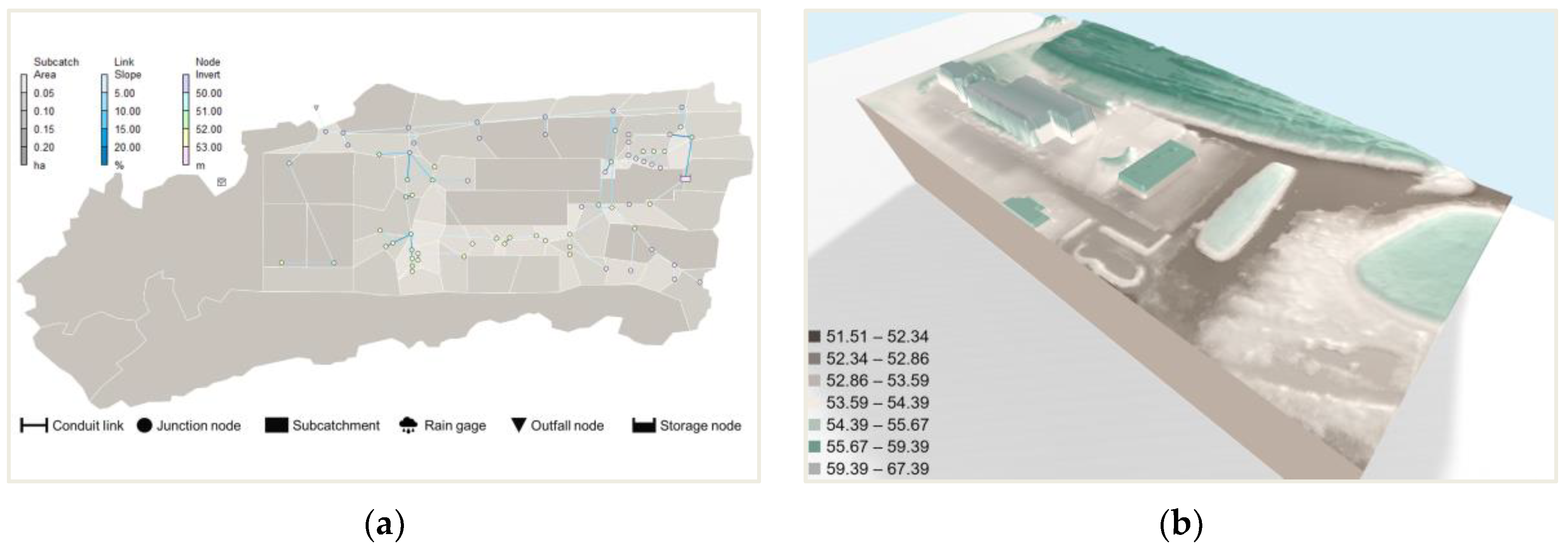
A land-use map and Google Maps were used to estimate the impervious ratio. Loss coefficients were set for square edge connections according to onsite data investigations [39]. The total precipitation depth was set to 55.00 mm according to the Euler-type II and the duration of event was selected to be one hour with time steps of five minutes. The precipitation model was built based on the KOSTRA-DWD 2010R report for the study area. This software contains the precipitation depths according to the German Weather Service specifications; the reference period of the reports are 1951 to 2010 [47]. This 100-year rain event was chosen since it corresponds to the selected rain event used by the city of Gelsenkirchen to create the official flood hazard map so that the results are comparable with it. Figure 3a displays the final SWMM model.
The main input of the LISFLOOD-FP model is the surface grid. The DEM of the study area were used as the primary grid; this grid was calibrated and validated using Google Maps and on-site measurements and photographs, resulting in the creation of a “height-corrected DEM” (Figure 3b). Manning’s coefficient of the surface was calculated automatically by employing QGIS. A uniform precipitation is also needed for setting up the LISFLOOD-FP model. DEM and precipitation model used in LISFLOOD-FP models are the same as the ones used for the SWMM model. Not all the calculation methods provided by the LISFLOOD-FP support an infiltration calculation, and when they do, a uniform infiltration rate is assumed across the floodplain; therefore, if applicable, the infiltration rate of the impervious area was preferred over the infiltration rate of the forests. The reason for this decision is the fact that in such heavy rain events, the pervious area starts behaving imperviously, and on the other hand, the main interest of the present thesis is urban areas where the surface is mostly impervious.
3. Results
3.1. Model Validation without Calibrating Data
3.1.1. SWMM
As discussed in Section 2.1 and Section 2.3, no data on the sewerage system performance were available, making a traditional calibration impossible. However, Huber and Cannon [45] have previously demonstrated that uncalibrated models can deliver valuable results provided that the hypotheses made during the model development are realistic. Moreover, for large events, only subcatchment properties, mainly the area and percentage of the impervious area, are dominant [40]. Therefore, the watershed discretization into subcatchments was carried out manually, since it provides the most accurate representation of the floodplain [37], combining the results of an automatic watershed delineation using QGIS and the results of the Thiessen polygon method on the sewerage system. These two delineations were combined manually based on the flow directions calculated using QGIS. The results of this combination were then validated and adjusted by several site surveys on dry (to check for possible obstructions that could divert the flow from its natural path) and wet days (to observe the surface runoffs’ natural patterns). The resulting model consists of 63 discrete SWMM subcatchments with uniform properties throughout each (Figure 3a). The discretized study area was then built in QGIS as a vector layer, which enabled an exact calculation of the area, maximum flow path length and slope for each subcatchment. Imperviousness ratios were calculated manually using Google Earth. The average calculated impervious percentage was 45.52%.
Geographical locations, elevations, and depths of the maintenance holes and drainage inlets (nodes) were controlled and validated by an onsite data investigation; the node lids were manually removed for the field measurements (node depths, node dimensions, the initial water depth of the nodes, conduit diameter, conduits’ direction toward the next node, and conduits’ inlet and outlet offsets from the ground surface). The node ground elevations were taken from the site plan and were compared with DEM elevation values; no deference was observed. Using Pythagoras’ theorem and the elevation of pipe fittings, the exact lengths of conduits were calculated.
3.1.2. LISFLOOD-FP
Two models were built and compared with each other for validating 2D models:
- Using raw DEM as the surface grid: aiming to select the most suitable inputs based on reference map values;
- Using the “height-corrected DEM” (Figure 3b) as the surface grid: aiming to select the most suitable surface grid based on field observations.
Raw DEM
In order to choose the optimal LISFLOOD-FP solver and Manning values, several simulations were run, and their results were compared with the reference map.
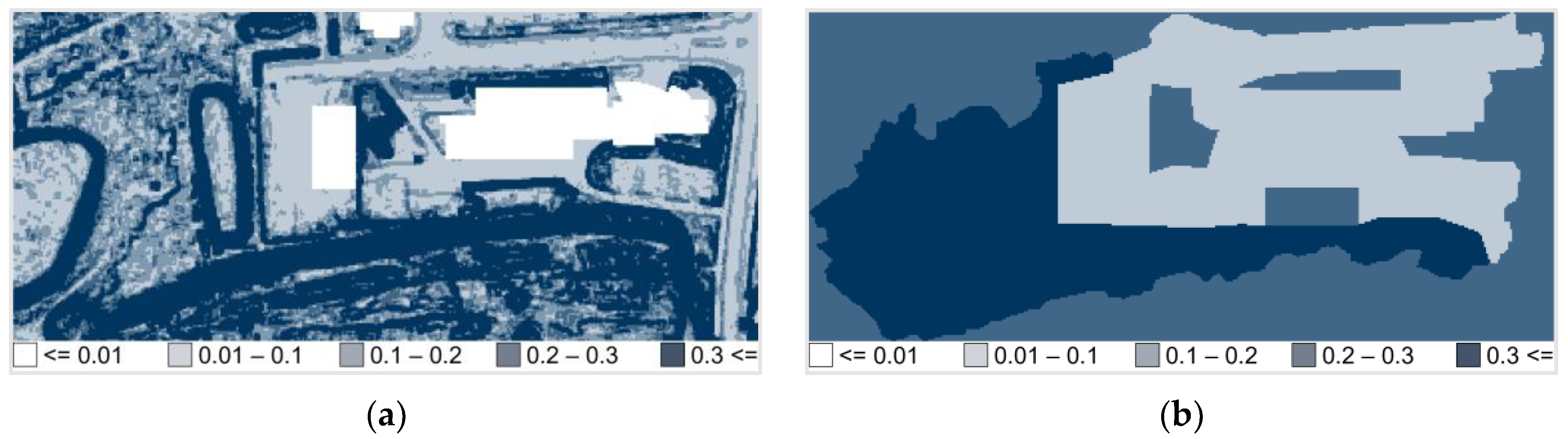
The calibration of the 2D models is often carried out by adjusting the roughness coefficient values; since such parameters were immeasurable, they had to be inferred by calibration. In order to achieve realistic roughness coefficient values without calibration data, using detailed, high-resolution DEM, which allows having a spatially distributed roughness coefficient, is recommended [48,49], using two sets of roughness coefficient values. One was computed automatically using QGIS [50] (Figure 4a), and the other one was generated using suggested values in the literature [40] (Figure 4b).
In addition to Manning values, a decision had to be made between LISFLOOD-FP solvers; consequently, four different maps were generated, combining both roughness values with both LISFLOOD-FP solvers.
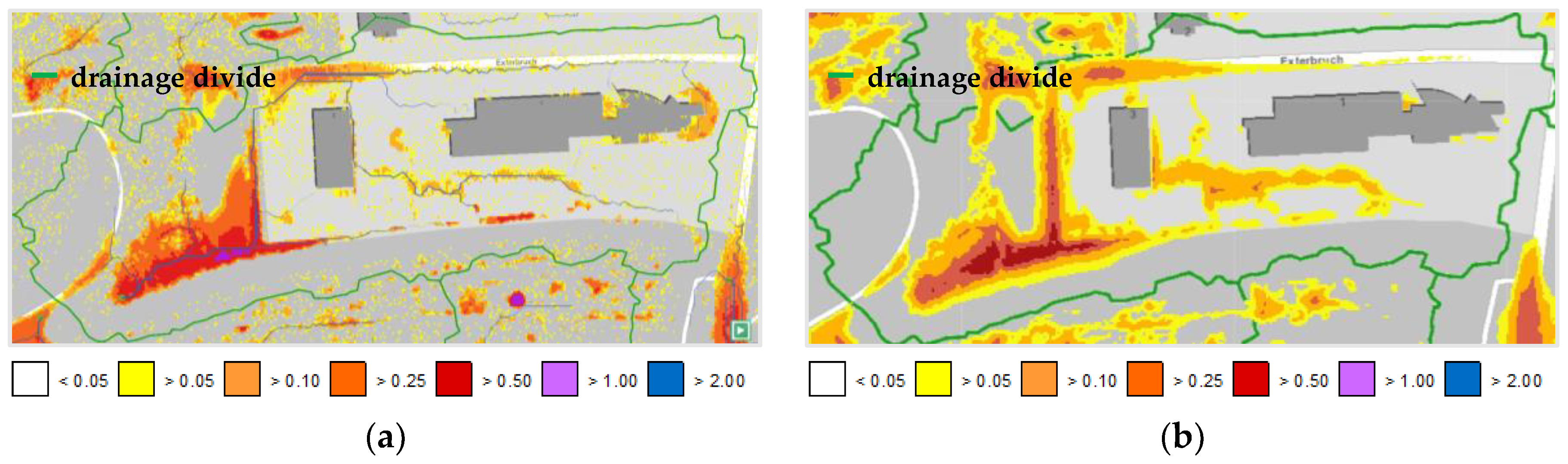
Figure 5 displays the flood map generated using the Roe solver, and the suggested roughness values from the literature [40] are on the right and on the left the reference map is shown. The results show an increase in the flood extent in the watershed’s non-urbanized area and a slight decrease in the water depths.
Figure 6 displays the flood map generated using the Roe solver, and the DEM-base roughness coefficient values are shown on the right and on the left the reference map is shown. The results show an increase in the flood extent and a decrease in the water depths.
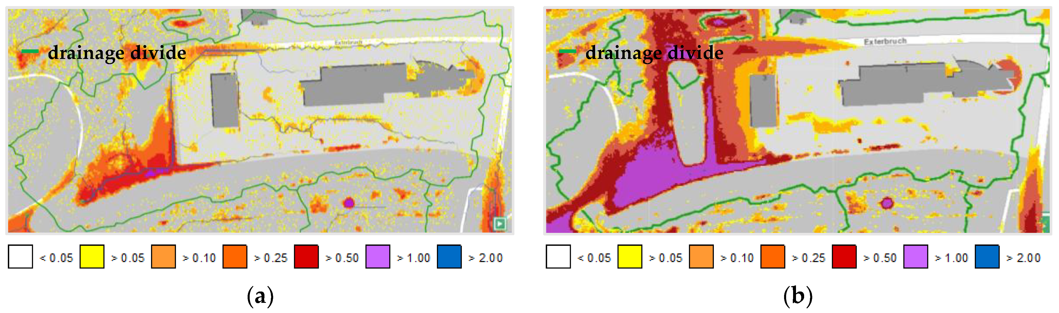
Figure 7 displays the flood map generated using the acceleration solver, and suggested roughness values from the literature are shown on the right and on the left the reference map is shown. The results show a significant increase in both flood extent and water depths.
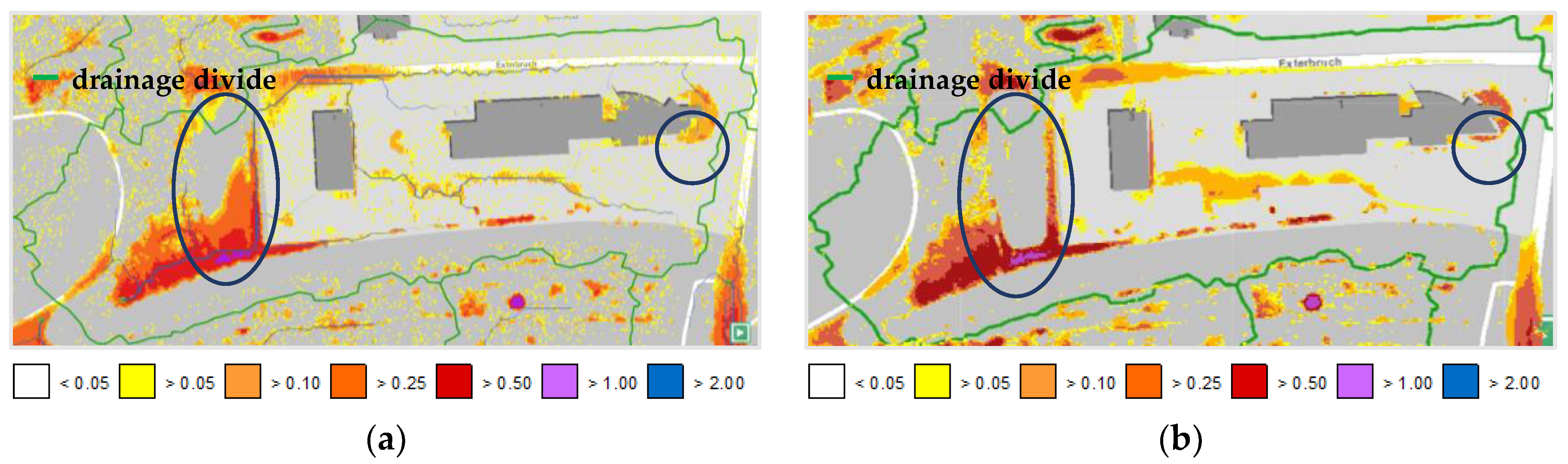
Figure 8 displays the flood map generated using the acceleration solver, and the DEM-base roughness coefficient is shown on the right and on the left the reference map is shown. As shown in the pictures, the predicted and reference maximum flooding depths and extents are very similar.
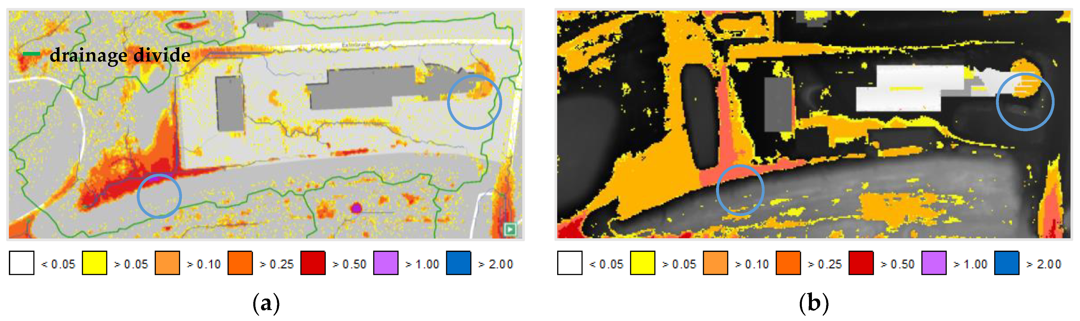
The two spots specified on each picture are the most apparent differences between the two maps; the one on the left is caused by the different GIS projections of the two maps; by overlaying the water depth layer on the original DEM file, this can clearly be seen (Figure 9a).
The other difference is in the artificial pond location; the water depth in the simulated map is higher than the reference map and can be explained by the existing water in the pond (Figure 9b).
The simulation results show that the acceleration solver combined with the DEM-base roughness values can deliver the most accurate results; accordingly, this approach was chosen for the rest of the work.
Height-Corrected DEM
Figure 10 shows the flood map generated by using height-corrected DEM as the surface grid and the reference map side by side. It can be seen that the predicted flood depth and extent are not similar to the reference map predictions. There is a decrease in the calculated water depth and an increase in the flood extent, especially in the watershed downstream.
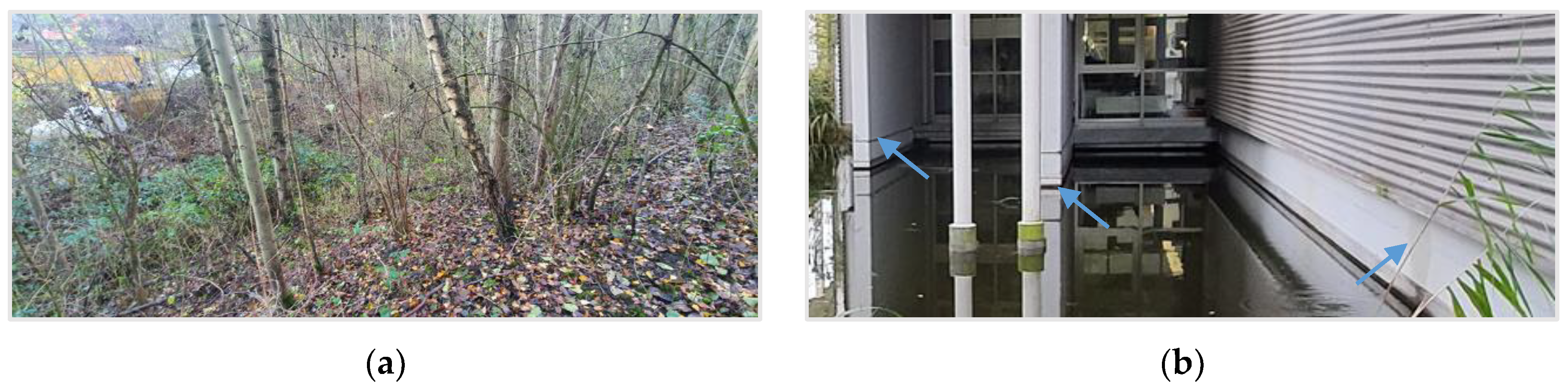
A comprehensive field investigation was conducted to find out which surface model provides the most realistic results. Two significant differences between the reference map and the map generated by the LISFLOOD-FP are marked (Figure 10). The left spot has a water depth between 1 and 2 m in the reference map, which indicates a significant difference in water depth between this spot and its surroundings. This difference is reasonable considering that the DEM cells in this spot lay about 1.5 m below its surrounding cells (thus, a sudden change in elevation on the surface occurs, which should be easy to see). Figure 11a is a picture of this spot, showing that the elevation changes smoothly, and there is no hole with around 1.5 m depth where the water would be stuck and collected; consequently, the water will flow all over the surface, resulting in a smaller depth and a larger extent. The second area specified on the right side of the maps (Figure 10) is where the artificial pond lies. Figure 11b shows the pond’s front view. As demonstrated in the photo, there are only three walls in the pond and not a solid part of the building.
Once the field survey was carefully carried out, all the differences between the two maps could be explained by these two reasons. In conclusion, using height-corrected DEM leads to more accurate results.
3.2. Model Performance
3.2.1. SWMM
Figure 12a shows the results after the model precipitation ends; SWMM estimates a total of 11.5 mm infiltration and 34.2 mm surface runoff for the entire rain duration. As expected, subcatchment number 62 has the maximum runoff with a total depth of 216.04 mm.
As reported by SWMM, 19 of the 70 junctions overflowed during the simulated precipitation. The maximum overflow rate was observed 24 min after the start of precipitation, applicable to all the 19 flooded junctions (the precipitation model reached its maximum intensity after 20 min). The maximum overflow rate occurred at J5, which collects the surface runoff of its allocated subcatchment (subcatchment 45) plus rainwater drained towards it by a downspout (Figure 12b). As an obvious result, this junction has the maximum total flood volume of around 20 m3.
Since no ground truth is available, the results’ plausibility can be judged by rational weighing of the predictions: the surface runoff in the urbanized part of the watershed starts almost as soon as the precipitation hits its peak, while at this point the non-urbanized part of the watershed is not flooded. In the non-urbanized area, surface runoff starts towards the end of the precipitation, while at this point there is no significant runoff in the urbanized area. These results can be justified on the one hand by the infiltration role in the non-urbanized area, and on the other hand, by the sewerage system constantly collecting the surface water in the urbanized area causing the excess surface runoff to be drained back to the drainage system after the precipitation intensity starts to decline.
3.2.2. LISFLOOD-FP
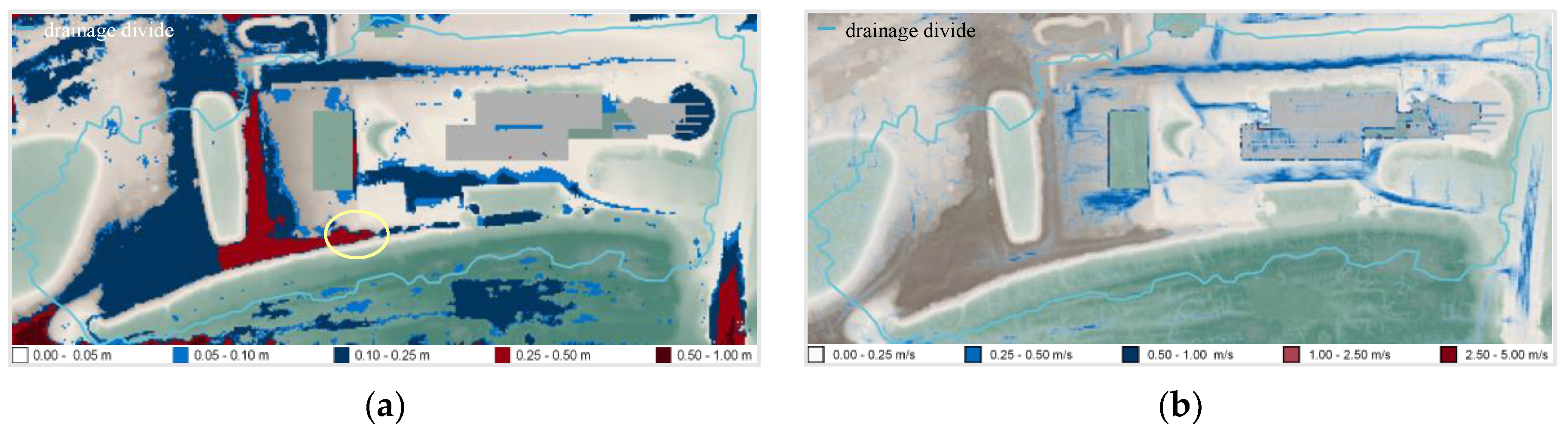
Figure 13a shows the results after the model precipitation ends. LISFLOOD-FP estimates the maximum water depth to be 301 mm (shown by the yellow outline).
Figure 13b displays the simulation outcomes for the maximum water velocities. The maximum velocities along the x-axis and y-axis are 2.42 m/s and 3.29 m/s, respectively. The map shows that the flow moves with a higher speed on smooth surfaces with uniform slopes, such as streets. The maximum velocities occur at the rooftop edges due to the sudden change in height; these kinds of high-velocity flows appear in single cells, whereas the relatively high-velocity flows on street surfaces happen in a series of neighboring cells.
3.3. Microscale Modeling
In this section, spots with the maximum runoff in each model have been chosen for a microscale analysis under the same conditions presented in Section 2, and the new outcomes of model validations (Section 3.1). The results were unacceptable and a considerable difference between the obtained result and the original result was observed (for SWMM a 100-percent continuity error and no surface runoff, and for LISFLOOD-FP the 55 mm precipitation turned into a uniform surface runoff of 50 mm and a uniform infiltration of 5 mm). Even before implementing this step, it was obvious that isolating a part of the watershed without considering the effect of its environment is not the correct way to assess the capability of SWMM and LISFLOOD-FP for microscale modeling. In an ideal world, where datasets would all be free access, an entire hydrological unit could be necessary to examine the capability of the models without any issue. On the other hand, an imaginary watershed model which is small yet complete can also be necessary and useful when these datasets are not available. To achieve this, the widths and the length of the understudy area and its components were multiplied by 0.1, since only the parameters in the X&Y direction were downsized, and so it was possible for the downsized model to use the same rain intensity and infiltration, considering that these parameters only deal with the Z direction, which stays unchanged. The purpose of this is to be able to compare the results of downsized models with the original models.
3.3.1. SWMM
Downsizing the subcatchments was carried out simply by downsizing the surface dimensions. Difficulties arose while working on the drainage system. Initially, the height and cross-sectional area of the nodes, as well as the length and cross-sectional area of the conduits, were multiplied by 0.1. However, this led to unreasonable results. As an alternative solution, only the radius of the conduits and nodes were multiplied by 0.1, although this method does not visually reduce the length and width of the initial model but since the model is conceptual, results would be comparable to the original ones. This reduces the drainage system’s capacity by 0.01, while the slope and height of the pipes and nodes do not change.
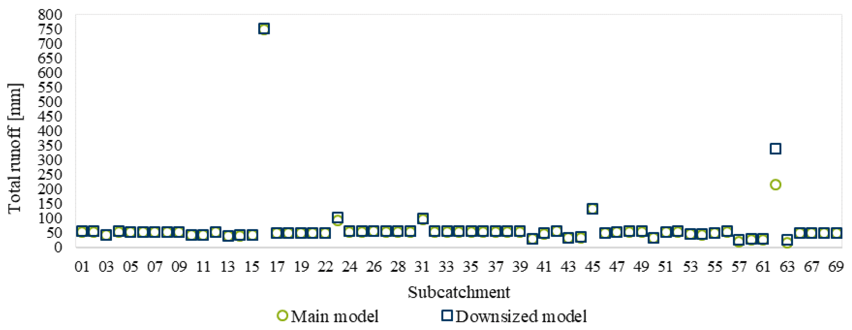
The comparison between the downsized model and the original model, shows that the predicted infiltration values in the two models are exactly equal, and the peak runoff volume value is exactly 0.01 of the peak runoff volume value in the initial model, meaning that the same peak runoff depth was predicted. Unlike these predictions, the total runoff depth was not exactly equal between the two models. Figure 14 shows the runoff depth recorded for both models. As shown in the diagram, subcatchment numbers 23, 57, 62, and 63 have the most significant difference in the amount of runoff depth predicted by the main model and runoff depth predicted by the downsized model. It is noteworthy that all four subcatchments are located in pervious areas, and there is not much difference in the urbanized regions.
According to the SWMM report, 25 of the 70 nodes overflow within the course of the simulation, including all the 19 flooded junctions of the original model. The extra six nodes have one thing in common: a field investigation was not possible for them. This implies that the smaller the modeling area, the higher the sensitivity to data accuracy. The downsized model’s peak flooding time was the same as the original model, 24 min after the model rainfall starts, for all nodes.
Other predictions for the drainage system had a notable difference compared to the original model, and no particular pattern for these differences was detected. Of course, the drainage system is a closed system, and the above-mentioned dissimilarities to the original model affect other acquired results; additionally, it was not possible to minimize all drainage system components by exactly 0.1; as a result, a numerical comparison between the original model’s predicted values and the downsized model is not logical in this case.
Despite all the hypotheses and inaccuracies made during the downsizing of the model, the downsized model accurately identified critical points so that closer and more accurate investigations could be carried out in real-time cases. Moreover, predicted flooding peak times were also the exact same as the ones for the original model in Section 3.2.1 (24 min after the rainfall begins).
3.3.2. LISFLOOD-FP
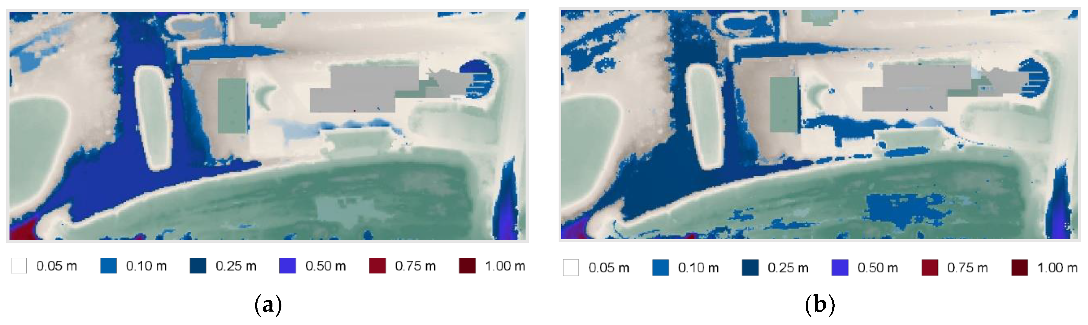
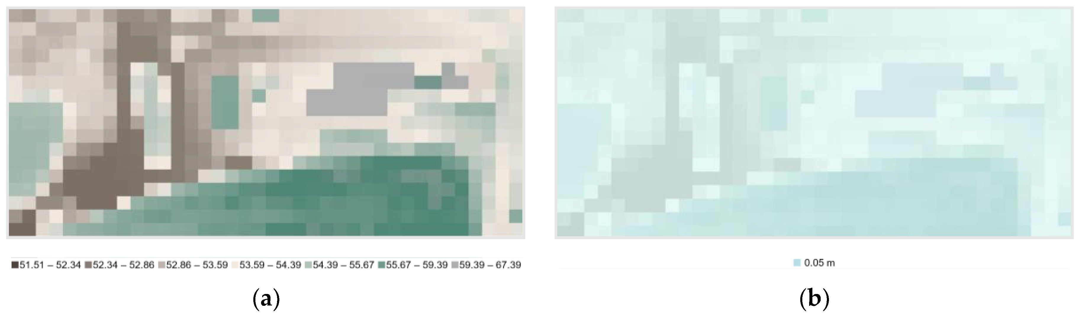
In order to downsize the study area, the length and width of the corrected DEM were reduced by ten times. The resulting DEM had a resolution of 1 cm, a length of 37.6 m and a width of 16.7 m. Attempts were made not to change cell heights, but in the process, some inevitable impreciseness occurred. The downsized model elevation varied from 51.53 m to 67.31 m, while the original watershed elevation varied from 51.51 m to 67.39 m. Figure 15 shows the result of the downsized model next to the result of the original model. As can be seen in this figure, the downsized model has been able to acceptably predict the flood extent. There is a slight difference in the flood depth, which may be due to impreciseness in the downsizing process.
The downsized watershed results predict an average of 5.23 cm water depths for the entire area after the precipitation ends, whereas the original model results suggest an average water depth of 5.05 cm after the precipitation ends.
Figure 16 shows the result of repeating all the steps for a second time. This time, the DEM of the downsized watershed had a resolution of one meter.
Although a one-meter DEM resolution is enough for modeling relatively large areas, it resulted in strongly unrealistic predictions for the microscale model (Figure 16a). The simulation result of the downsized watershed with one-meter DEM predicts a uniform water depth of 5 cm for the entire domain (Figure 16b).
4. Discussion
4.1. Are the Results of These Products Rational?
The comparison between the results of the LISFLOOD-FP and the reference map shows that the results obtained for the two-dimensional LISFLOOD-FP surface model are reasonable. It allows the conclusion that both models behave quite similarly in terms of water level and flood extent, provided the calculation method and input data are appropriately selected. This is a very positive outcome, as the free model compares well to the one used for the flood map (more expensive and sophisticated one).
The evaluation of the runoff predicted by the SWMM is not as easy as the LISFLOOD-FP. Because the SWMM has mainly been designed to model the drainage system and the calculation of surface runoff in such a small watershed, it depends highly on the watershed division method. However, the quality of the results of the SWMM also rationally corresponds to the reference map. The highest runoff amount was predicted for subcatchment 62, exactly the same area predicted by the LISFLOOD-FP and the reference map as the most critical location. Additionally, in the urbanized area, the predicted runoff depth for subcatchments that do not directly access the drainage system or receive runoff from adjacent subcatchments is higher than other subcatchments. Although these results obtained by the SWMM model correspond to the reference map and the site observation results, it is noteworthy that these results depend largely on the watershed division method. In fact, in this project, the watershed is divided according to the frequent observations of the watershed on rainy days and also the use of QGIS to accurately discretize the surface and predict the surface flow paths so that non-numerical results obtained for the watershed were predictable before the running of the model.
For the entire watershed, the SWMM has calculated an average maximum water depth of 34.2 mm, while the average maximum water depth calculated by the LISFLOOD-FP is 59.1 mm. Considering that the first model transfers a part of the generated runoff by the drainage system, the difference of two centimeters can be justified for the runoff produced by these two models.
The results of the SWMM model for the drainage system are conceptually in accordance with the observations made. Nodes that are downstream relative to their adjacent nodes, as well as nodes that have less capacity than the runoff volume they collect, overflow. Nevertheless, due to the lack of observational data, it is impossible to statistically assess the flooding volume.
This model could also show the effect of soil infiltration reasonably. In impervious urban environments, the highest flow rate occurs after precipitation reaches its maximum, but in non-urban environments, the highest flow rate occurs when the soil’s infiltration capacity is depleted.
4.2. Are the Input Parameters of these Products Adjustable to Achieve Realistic Results?
Most of the input data of both models are adjustable and allow the user to calibrate them. However, some input data that can have a significant effect on the results cannot be adjusted.
In the SWMM, all the data used in this research are adjustable except for some node specifications. In the SWMM model, the program does not provide any capability to consider node covers; this may not have much effect in simulating large areas. However, it should be considered when examining small watersheds in great detail. There is also no option to define pipe fittings, and the junction option must be used to create them in the model. In order to prevent flooding in pipe fitting junctions, a surcharge depth higher than the maximum expected hydraulic depth in the whole system should be set. This type of node modeling causes minor inaccuracies in the depth of the nodes as well as the length of the conduits. Furthermore, the entrance area of the junctions is not adjustable for each junction, but the SWMM model considers a single adjustable value as the area for all junctions.
The LISFLOOD-FP model is an uncomplicated model that, in some cases, does not allow the users to make changes. In this model, precipitation, as well as infiltration, are considered uniformly throughout the modeling area. Due to the small size of the area studied and the high intensity of the selected rain model, these two inefficiencies did not negatively affect the model results. However, they could cause inaccuracies when modeling large regions and spatially non-uniform precipitations. Another noteworthy point in this model is that the cell dimensions are unchangeable and uniform and depend on the DEM resolution. On the one hand, it causes an increase in the number of cells required to achieve comparable accuracy to models that allow having a non-uniform grid; consequently, it causes an increase in computing time to achieve the desired accuracy, and on the other hand, when only a part of the domain has better resolution and demands more data accuracy, but the high-resolution DEM is not available for the other parts of the domain, the high-resolution DEM must be resampled so that its resolution matches with the resolution of the rest of the domain, which can lead to a decrease in the result’s accuracy.
4.3. Are the Models User-Friendly?
In order to build a model of the drainage network, i.e., junctions and conduits, the software is very efficient and easy to work with, but to prepare subcatchments, it is necessary to use other GIS software products, which means that in addition to this model, the user must work with another software. Alternatively, the user may define the subcatchments according to personal knowledge, which, to some extent, increases the probability of inaccuracy. The software manual also does not provide sufficient and applicable information on the practical methods of dividing the domain into subcatchments. In this study, the watershed division, defining them in the model, and determining the parameters of each subcatchment was the most time-consuming part of the whole work. The most significant advantage is the fact that the software is open source, yet it can easily compete with other 1D models.
A LISFLOOD-FP model is simple to create and run since it has a relatively straightforward design, diverse simulation methods, is computationally efficient, and acceptable to non-professionals. Similar to the SWMM, the model is open source and provides the possibility to achieve acceptable results for researchers who cannot access or afford commercial products. LISFLOOD-FP gives the user the option to choose between different SWE simplifications based on their modeling goals. The DEM data need pre-processing, which requires the user to employ GIS products. Some error warnings will not be notified to the user and just ignored by the LISFLOOD-FP; for instance, if the model does not recognize some parameters, there will be no warnings. As a result, in case of a typo in one of these parameters, it will be ignored instead of being addressed by the program, which can cause severe problems with interpreting the results.
4.4. Are These Products Time Consuming in Terms of Pre-Processing, Computational, and Post-Processing Time?
In general, building one-dimensional models is more time consuming than building two-dimensional models because the latter only needs the reconstruction of the overland surface where water could run; however, for the one-dimensional models, more details are requested (slope, roughness, dimensions, angles, connections, etc.). The lack of access to a GIS module in SWMM makes it necessary to use another software, which greatly increases the surface data preparation time. In order to calculate the parameters of each subcatchment, such as width, area, and slope, it was necessary to use QGIS. In addition to the time required to prepare this data and transfer it from the QGIS to this model was time consuming, and to prevent errors during data transfer, it was necessary to check and control this step several times.
The calculation time for this model is very short, and due to modeling a small area, it is not possible to comment much on it because, in the simulation of small domains, the calculation time is not a serious issue; instead, the accuracy of the input data is much more critical.
The SWMM model results are not easily understandable or usable by the general public and require further processing (no hazard map would be generated). The software itself does not carry out this processing, but other methods and software products must be used to draw a general conclusion from the outputs. Although this step is not undertaken in this study because it was not intended to be, it could be time consuming; additionally, transferring data from one software to another can be time consuming and a source of error.
The similarity between the LISFLOOD-FP and the SWMM is that both models need a GIS product to prepare the inputs; working with this model also requires a very basic understanding of programming concepts, which are relatively simple to learn. Although the model itself provides an executable to see the simulation results, the executable is of very low quality and is practically unusable due to repeated errors. Moreover, the results provided by this model are in particular text file formats, so that the QGIS was needed to gain a visual understanding of them. However, it can be said that if the user has sufficient knowledge of the selected GIS product, the pre-processing and post-processing are basic and not time consuming. If the outcomes do not need further analysis and a simple overview of flooding hotspots is enough for the user, the executable meets the user’s need.
4.5. Are These Products Suitable for Microscale Modeling?
This question’s answer depends more on the input data and their accuracy and level of detail than on the software used. In the first software review, it was observed that when a minimal area without considering the surrounding conditions was examined, or even when the inflows from the rest of the watershed were added to the model, the results obtained did not reflect the reality. Nevertheless, when investigating a region with the same surface area but encompassing an entire watershed and sewershed, meaning that it has a complete drainage system, upstream, downstream, and outlet, the answers are much closer to reality. From these outcomes, it can be concluded that for modeling a small environment, the accuracy of the data, as well as the surrounding conditions that affect this environment, must be considered.
The results obtained from the LISFLOOD-FP are the same as the SWMM, with the one difference that the results showed that in the two-dimensional model when a complete watershed but with a very small surface area is modeled, the obtained results are very similar to the results shown in the reference map, and there is little difference in the results obtained for these two models in terms of flood depth and extent.
It is noteworthy that when downsizing the original model, the resolution of the model also increased, while when the same step was undertaken without increasing the resolution of the DEM, the results were significantly different from the original model. In general, it can be concluded from the results obtained that for this watershed, as the area becomes smaller, the accuracy of the data, the details of the watershed, and the environmental conditions become more effective.
4.6. Are the Freeware Products Suitable for the Commercial Companies?
Choosing the right model depends first and foremost on the purpose of the research. If the user necessarily requires using a 1D/2D model, unfortunately, freeware products are not a robust option, although much effort has been made in this area and in many cases an in-house model has been developed by researchers across various institutions. However, if the requirements are met by using one-dimensional or two-dimensional models, the user’s needs can be met by applying a few adjustments.
Since freeware products are sometimes time consuming due to the lack of direct access to some features such as a GIS module or due to having no or very basic customer services, and due to the need for basic knowledge in related fields from time to time, the commercial sectors should consider whether it is better to pay for the human resources or spend on a commercial software product. Additionally, regardless of which software is chosen, it is better to collect all the data with the necessary accuracy and details, i.e., to provide the same or better accuracy as desired for the outputs for the inputs and to avoid uncertainties caused by making modeling assumptions and using recommended values instead of collecting the required data.
5. Conclusions
Gathering detailed hydrological and hydraulic data that can be used for the assessment of existing and new drainage systems, as well as for the creation of flood maps, can be challenging, particularly for users in DCs. As a consequence, there is a strong need to identify tools and approaches that do not demand detailed data for generating reliable results. To address this issue, this paper aimed to compare the performance of two existing free tools, LISFLOOD-FP and SWMM, for a specific case scenario of a small watershed with scarce data available. Their outcomes were validated with observations made in the field and simulations were made at the scale of a building (microscale), aiming to assess urban flood modeling at different scales while facing resource paucity and providing some suggestions for future approaches within similar situations. The major outcomes obtained with this study can be summarized as follows.
- Free numerical tools can compete with paid commercial ones; however, the pre- and post-processing times are typically longer, and it should also be mentioned that these products can be used for 2D models, without reaching the accuracy that more realistic and robust 1D/2D paid models are able to achieve. Freeware products make some simplifications in their modeling approach such as taking a uniform infiltration or precipitation into account, which can lead to inaccuracies; however, this study demonstrated that this limitation can be solved by discretizing the study area manually by the user;
- This work has shown that by putting extra attention and effort into collecting even limited, targeted and specific input data, reasonable results can still be generated, especially if what is needed should have been used for the calibration process;
- Finally, generating essential information about a specific area or at the microscale is dependent on the resolution of the provided input data, and this is valid for both freeware and commercial tools. However, this study demonstrated that, even with an initial lack of input datasets, freeware products are able to produce high-resolution results, even if not at a large scale but at local points.
Flood modeling is a crucial tool in developing policies for flood risk management. The data paucity, the lack of access to resources and the missing high-resolution data to be used in models are all issues affecting DCs, especially in Asia and Africa, rather than developed countries such as the Netherlands, United Kingdom and the United States. The cause for this uncertain situation of information could be due to reasons linked with a lack of funds or political influence. Parameters such as flood depth, inundation extent, inundation time and water flow velocity are crucial, together with topographical data, and should also be of a high-resolution and offer the spatial domain for assessing flood risk. This study demonstrated that LISFLOOD-FP and SWMM can cope with the lack of these variables as a starting point and has provided steps to undertake to generate reliable results for the need required, which is the estimation of the impacts of flooding events and the likelihood of their occurrence.
Author Contributions
Conceptualization, F.S., M.G. and M.R.; methodology, F.S., M.G. and M.R.; software, F.S.; validation, F.S.; formal analysis, F.S., M.G. and M.R.; investigation, F.S., M.G. and M.R.; resources, F.S. and M.G.; data curation, F.S. and M.R.; writing—original draft preparation, F.S. and M.R.; writing—review and editing, F.S., M.G., J.H. and M.R.; visualization, F.S.; supervision, M.G. and M.R.; project administration, M.G. All authors have read and agreed to the published version of the manuscript.
Funding
This research received no external funding.
Institutional Review Board Statement
Not applicable.
Informed Consent Statement
Not applicable.
Data Availability Statement
To access the datasets, please contact Farzaneh Sadeghi.
Acknowledgments
The authors would like to kindly thank Professor Bert Boessler for his support, his technical contribution and his assistance during the entire study. He is an inspiration to all of us.
Conflicts of Interest
The authors declare no conflict of interest.
References
- Rubinato, M.; Nichols, A.; Peng, Y.; Zhang, J.; Lashford, C.; Cai, Y.; Lin, P.; Tait, S. Urban and river flooding: Comparison of flood risk management approaches in the UK and China and an assessment of future knowledge needs. Water Sci. Eng. 2019, 12, 274–283. [Google Scholar] [CrossRef]
- Rubinato, M.; Luo, M.; Zheng, X.; Pu, J.H.; Shao, S. Advances in modelling and prediction on the impact of human activities and extreme events on environments. Water 2020, 12, 1768. [Google Scholar] [CrossRef]
- Jha, A.K.; Bloch, R.; Lamond, J. Cities and Flooding: A Guide to Integrated Urban Flood Risk Management for the 21st Century; Abhas, K., Jha, R., Lamond, J., Eds.; World Bank: Washington, DC, USA, 2012; ISBN 978-0821388662. [Google Scholar]
- Wu, X.; Wang, Z.; Guo, S.; Lai, C.; Chen, X. A simplified approach for flood modeling in urban environments. Hydrol. Res. 2018, 49, 1804–1816. [Google Scholar] [CrossRef]
- Convery, I.; Bailey, C. After the flood: The health and social consequences of the 2005 Carlisle flood event. J. Flood Risk Manag. 2008, 1, 100–109. [Google Scholar] [CrossRef]
- Galloway, G.E.; Reilly, A.; Ryoo, S.; Riley, A.; Haslam, M.; Brody, S.; Highfield, W.; Gunn, J.; Rainey, J.; Parker, S. The Growing Threat of Urban Flooding: A National Challenge; University of Maryland: College Park, MD, USA, 2018. [Google Scholar]
- FloodList. Available online: https://floodlist.com/news (accessed on 12 September 2021).
- Beden, N.; Ulke Keskin, A. Flood map production and evaluation of flood risks in situations of insufficient flow data. Nat. Hazards 2021, 105, 2381–2408. [Google Scholar] [CrossRef]
- Bosseler, B.; Salomon, M.; Schlüter, M.; Rubinato, M. Living with urban flooding: A continuous learning process for local municipalities and lessons learnt from the 2021 events in Germany. Water 2021, 13, 2769. [Google Scholar] [CrossRef]
- Rubinato, M.; Shucksmith, J.; Saul, A.J.; Shepherd, W. Comparison between InfoWorks hydraulic results and a physical model of an urban drainage system. Water Sci. Technol. 2013, 68, 372–379. [Google Scholar] [CrossRef] [PubMed] [Green Version]
- Rubinato, M.; Martins, R.; Kesserwani, G.; Leandro, J.; Djordjević, S.; Shucksmith, J. Experimental calibration and validation of sewer/surface flow exchange equations in steady and unsteady flow conditions. J. Hydrol. 2017, 552, 421–432. [Google Scholar] [CrossRef]
- Rubinato, M.; Martins, R.; Shucksmith, J.D. Quantification of energy losses at a surcharging manhole. Urban Water J. 2018, 15, 234–241. [Google Scholar] [CrossRef] [Green Version]
- Martins, R.; Kesserwani, G.; Rubinato, M.; Lee, S.; Leandro, J.; Djordjević, S.; Shucksmith, J.D. Validation of 2D shock capturing flood models around a surcharging manhole. Urban Water J. 2017, 14, 892–899. [Google Scholar] [CrossRef]
- Ming, X.; Liang, Q.; Xia, X.; Li, D.; Fowler, H.J. Real--time flood forecasting based on a high--performance 2--D hydrodynamic model and numerical weather predictions. Water Resour. Res. 2020, 56, e2019WR025583. [Google Scholar] [CrossRef]
- Kharat, D.B. Practical Aspects of Integrated 1D2D Flood Modelling of Urban Floodplains Using LiDAR Topography Data. Ph.D. Thesis, Heriot-Watt University, Edinburgh, UK, 2009. [Google Scholar]
- Di Baldassarre, G. Floods in a Changing Climate: Inundation Modelling, 1st ed.; Cambridge University Press: Cambridge, UK, 2017; ISBN 9781108446754. [Google Scholar]
- Martins, R.D. Development of a Fully Coupled 1D/2D Urban Flood Model. Ph.D. Thesis, University of Coimbra, Coimbra, Portugal, 2015. [Google Scholar]
- Bulti, D.T.; Abebe, B.G. A review of flood modeling methods for urban pluvial flood application. Model. Earth Syst. Environ. 2020, 6, 1293–1302. [Google Scholar] [CrossRef]
- Leandro, J. Advanced Modelling of Flooding in Urban Areas: Integrated 1D/1D and 1D/2D Models. Ph.D. Thesis, University of Exeter, Exeter, UK, 2008. [Google Scholar]
- Ochoa-Rodríguez, S. Urban pluvial flood modelling: Current theory and practice: Review document related to Work Package 3—Action 13; RainGain: London, UK, 2013. [Google Scholar]
- Leandro, J.; Chen, A.S.; Djordjević, S.; Savić, D.A. Comparison of 1D/1D and 1D/2D coupled (sewer/surface) hydraulic models for urban flood simulation. J. Hydraul. Eng. 2009, 135, 495–504. [Google Scholar] [CrossRef]
- Henonin, J.; Russo, B.; Mark, O.; Gourbesville, P. Real-time urban flood forecasting and modelling—A state of the art. J. Hydroinf. 2013, 15, 717–736. [Google Scholar] [CrossRef]
- Kesserwani, G.; Lee, S.; Rubinato, M.; Shucksmith, J. (Eds.) Experimental and Numerical Validation of Shallow Water Flow around a Surcharging Manhole. In Proceedings of the 10th Urban Drainage Modelling Conference, Mont-Sainte Anne, QC, Canada, 20–23 September 2015; UDM2015.org. pp. 145–154. [Google Scholar]
- Garcıa-Navarro, P.; Brufau, P.; Burguete, J.; Murillo, J. The shallow water equations: An example ofhyperbolic system. Monogr. Real Acad. Cienc. Zaragoza 2008, 31, 89–119. [Google Scholar]
- Rubinato, M.; Lashford, C.; Goerke, M. Advances in experimental modelling of urban flooding. In Water-Wise Cities and Sustainable Water Systems: Concepts, Technologies, and Applications; Xiaochang, C., Guangtao, F., Wang, X.C., Fu, G., Eds.; IWA Publishing: London, UK, 2020; pp. 235–257. ISBN 9781789060768. [Google Scholar]
- Norallahi, M.; Seyed Kaboli, H. Urban flood hazard mapping using machine learning models: GARP, RF, MaxEnt and NB. Nat. Hazards 2021, 106, 119–137. [Google Scholar] [CrossRef]
- Bermúdez, M.; Zischg, A.P. Sensitivity of flood loss estimates to building representation and flow depth attribution methods in micro-scale flood modelling. Nat. Hazards 2018, 92, 1633–1648. [Google Scholar] [CrossRef] [Green Version]
- Ernst, J.; Dewals, B.J.; Detrembleur, S.; Archambeau, P.; Erpicum, S.; Pirotton, M. Micro-scale flood risk analysis based on detailed 2D hydraulic modelling and high resolution geographic data. Nat. Hazards 2010, 55, 181–209. [Google Scholar] [CrossRef]
- Wetterdienst.de. Klima Gelsenkirchen—Wetterdienst.de. Available online: https://www.wetterdienst.de/Deutschlandwetter/Gelsenkirchen/Klima (accessed on 12 September 2021).
- Stadt Gelsenkirchen. Starkregengefahrenkarte: © GeoBasis-DE / BKG 2021 | © Stadt Gelsenkirchen (2021), Datenlizenz Deutschland – Zero – Version 2.0 (www.govdata.de/dl-de/zero-2-0) | © Stadt Gelsenkirchen (2021), Datenlizenz Deutschland - Namensnennung - Version 2.0 (www.govdata.de/dl-de/by-2-0) | © con terra GmbH. Calculated by Ingenieurbüro Dr. Pecher AG, Erkrath. Available online: https://gdi.gelsenkirchen.de/mapapps/resources/apps/UN_003/index.html?lang=de#/ (accessed on 5 September 2021).
- Bundesamt für Kartographie und Geodäsie-2021. Verwaltungsgebiete 1:5,000,000 (Ebenen), Stand 01.01. (VG5000 01.01.): © GeoBasis-DE/BKG (2022). Data Licence Germany—Attribution—Version 2.0. Available online: https://daten.gdz.bkg.bund.de/produkte/vg/vg5000_0101/aktuell/vg5000_01-01.utm32s.shape.ebenen.zip (accessed on 20 February 2022).
- Opendata.Gelsenkirchen.de. Verwaltungsgrenzen der Stadt Gelsenkirchen (WMS & WFS): © 2022 Ministerium für Wirtschaft, Innovation, Digitalisierung und Energie des Landes Nordrhein-Westfalen. Data licence Germany—Attribution—Version 2.0. Available online: https://gdi.gelsenkirchen.de/karten/GB_Geobasis/Verwaltungsgrenzen/download/Verwaltungsgrenzen_SHP.zip (accessed on 20 February 2022).
- Google Maps. Google Satellite: CRS: EPSG:3857–WGS 84/Pseudo-Mercator–Projected: Kartendaten © 2020 GeoBasis-DE/BKG (©2009). Available online: https://mt1.google.com/vt/lyrs=s&x=%7Bx%7D&y=%7By%7D&z=%7Bz%7D (accessed on 3 October 2020).
- Néelz, S.; Pender, G. Benchmarking of 2D Hydraulic Modelling Packages; Environment Agency: Bristol, UK, 2010; ISBN 978-1-84911-190-4. [Google Scholar]
- Bates, P.; Roo, A. A simple raster-based model for flood inundation simulation. J. Hydrol. 2000, 236, 54–77. [Google Scholar] [CrossRef]
- Neal, J.; Schumann, G.; Bates, P. A subgrid channel model for simulating river hydraulics and floodplain inundation over large and data sparse areas. Water Resour. Res. 2012, 48. [Google Scholar] [CrossRef]
- Wu, Z.; Ma, B.; Wang, H.; Hu, C. Study on the improved method of urban subcatchments division based on aspect and slope—Taking SWMM model as example. Hydrology 2020, 7, 26. [Google Scholar] [CrossRef]
- Bates, P.; Dabrowa, A.; Fewtrell, T.; Neal, J.; Trigg, M. LISFLOOD-FP User Manual; University of Bristol: Bristol, UK, 2013. [Google Scholar]
- Elger, D.F.; LeBret, B.A.; Crowe, C.T.; Roberson, J.A. Engineering Fluid Mechanics, 11th ed.; International Student Version; Wiley: Singapore, 2016; ISBN 9781119249221. [Google Scholar]
- James, W.; Rossman, L.; James, R. User’s Guide to SWMM 5 13th Edition: Based on Original USEPA SWMM Documentation; CHI Press: Guelph, ON, Canada, 2010. [Google Scholar]
- itwh GmbH. KOSTRA-DWD 2010R; Deutsche Wetterdienst: Offenbach am Main, Germany.
- BGR. Bodenatlas. Available online: https://geoviewer.bgr.de/mapapps4/resources/apps/bodenatlas/index.html?lang=de&tab=boedenDeutschlands (accessed on 19 September 2021).
- Mirgel, M.; Wruck, O. 3D-Messdaten. Available online: https://www.bezreg-koeln.nrw.de/brk_internet/geobasis/hoehenmodelle/3d-messdaten/index.html (accessed on 6 September 2021).
- Mirgel, M.; Wruck, O. Digitales Geländemodell. Available online: https://www.bezreg-koeln.nrw.de/brk_internet/geobasis/hoehenmodelle/digitale_gelaendemodelle/gelaendemodell/index.html (accessed on 6 September 2021).
- Mirgel, M.; Wruck, O. ab 2003: Digitale Topographische Karte 1: 10,000. Available online: https://www.bezreg-koeln.nrw.de/brk_internet/geobasis/topographische_karten/historisch/ab-2003/index.html (accessed on 19 September 2021).
- Frechen, M. Loess in Europe: Guest editorial. E&G Quaternary Sci. J. 2011, 60, 3–5. [Google Scholar] [CrossRef]
- Itwh—Institut für Technisch-Wissenschaftliche Hydrologie GmbH. KOordinierte STarkniederschlags-Regionalisierungs-Auswertungen. © 2021 itwh GmbH. Available online: https://itwh.de/en/software-products/desktop/kostra-dwd-2010r/ (accessed on 21 February 2022).
- Bates, P.D. Remote sensing and flood inundation modelling. Hydrol. Process. 2004, 18, 2593–2597. [Google Scholar] [CrossRef]
- Mukolwe, M.M. Flood Hazard Mapping. Available online: https://ebookcentral.proquest.com/lib/gbv/detail.action?docID=4824779 (accessed on 19 September 2021).
- QGIS Documentation. 24.2.1. Raster Analysis. Available online: https://docs.qgis.org/3.16/en/docs/user_manual/processing_algs/gdal/rasteranalysis.html#gdalroughness (accessed on 12 September 2021).

Figure 2.
Study area: (a) Google Maps view [33]; (b) official flood map provided by the city of Gelsenkirchen [30].

Figure 3.
(a) Final model implemented in SWMM; (b) final surface model used in LISFLOOD-FP.

Figure 4.
Manning’s n values: (a) Roughness coefficient automatic generated by QGIS; (b) roughness coefficient based on suggested values in the literature.
Figure 4.
Manning’s n values: (a) Roughness coefficient automatic generated by QGIS; (b) roughness coefficient based on suggested values in the literature.

Figure 5.
Predicted flood extent and depth after the precipitation: (a) reference flood map [30]; (b) simulation using the Roe solver with the suggested roughness values in the literature.
Figure 5.
Predicted flood extent and depth after the precipitation: (a) reference flood map [30]; (b) simulation using the Roe solver with the suggested roughness values in the literature.

Figure 6.
Predicted flood extent and depth after the precipitation: (a) reference flood map [30]; (b) simulation using Roe solver with the DEM-base roughness coefficient values.
Figure 6.
Predicted flood extent and depth after the precipitation: (a) reference flood map [30]; (b) simulation using Roe solver with the DEM-base roughness coefficient values.

Figure 7.
Predicted flood extent and depth after the precipitation: (a) reference flood map [30]; (b) simulation using an acceleration solver, and the SWMM manual roughness coefficient values.
Figure 7.
Predicted flood extent and depth after the precipitation: (a) reference flood map [30]; (b) simulation using an acceleration solver, and the SWMM manual roughness coefficient values.

Figure 8.
Predicted flood extent and depth after the precipitation: (a) reference flood map [30]; (b) simulation using acceleration solver, and the DEM-base roughness coefficient values.
Figure 8.
Predicted flood extent and depth after the precipitation: (a) reference flood map [30]; (b) simulation using acceleration solver, and the DEM-base roughness coefficient values.

Figure 9.
Predicted flood extent and depth after the precipitation: (a) flood map on the surface model which was used for the simulation; (b) existing water in the artificial pond.
Figure 9.
Predicted flood extent and depth after the precipitation: (a) flood map on the surface model which was used for the simulation; (b) existing water in the artificial pond.

Figure 10.
Predicted flood extent and depth after the rain event: (a) reference flood map [30]; (b) simulation using acceleration solver, and the DEM-base auto-generated roughness coefficient values on the height-corrected DEM.
Figure 10.
Predicted flood extent and depth after the rain event: (a) reference flood map [30]; (b) simulation using acceleration solver, and the DEM-base auto-generated roughness coefficient values on the height-corrected DEM.

Figure 11.
Significant differences between the reference map and the map generated by the LISFLOOD-FP: (a) the area for which the DEM data were incorrect; (b) the front view of the structure in the pond.
Figure 11.
Significant differences between the reference map and the map generated by the LISFLOOD-FP: (a) the area for which the DEM data were incorrect; (b) the front view of the structure in the pond.

Figure 12.
(a) Calculation results after the model precipitation ends; (b) calculation results 24 min after the precipitation starts.
Figure 12.
(a) Calculation results after the model precipitation ends; (b) calculation results 24 min after the precipitation starts.

Figure 13.
(a) Flood hazard map of understudy watershed for a 100-year rain event with a duration of one hour generated by LISFLOOD-FP; (b) maximum predicted water velocities for a 100-year rain event.
Figure 13.
(a) Flood hazard map of understudy watershed for a 100-year rain event with a duration of one hour generated by LISFLOOD-FP; (b) maximum predicted water velocities for a 100-year rain event.

Figure 14.
The total runoff amount predicted by the original model compared to the total runoff amount predicted by the downsized model.
Figure 14.
The total runoff amount predicted by the original model compared to the total runoff amount predicted by the downsized model.

Figure 15.
Comparison of the downsized model with the original model: (a) flood hazard map of the downsized model for a 100-year rain event with a duration of one hour generated by LISFLOOD-FP; (b) flood hazard map of the original model for a 100-year rain event with a duration of one hour generated by LISFLOOD-FP.

Figure 16.
Downsizing the model without increasing the DEM resolution: (a) DEM of the downsized watershed with a resolution of one meter; (b) predicted hazard map for the downsized watershed with a DEM resolution of one meter.
Figure 16.
Downsizing the model without increasing the DEM resolution: (a) DEM of the downsized watershed with a resolution of one meter; (b) predicted hazard map for the downsized watershed with a DEM resolution of one meter.


Table 1.
An overview of data sources.
| Data | Provider |
|---|---|
| Sewerage system | site-specific surveying, Computer-Aided Design (CAD) maps |
| Losses | engineering fluid mechanics [39] |
| Depression storage depth | user’s guide to SWMM [40] |
| Manning’s coefficient | user’s guide to SWMM [40], QGIS |
| Infiltration parameter | user’s guide to SWMM [40] |
| Precipitation | KOSTRA-DWD 2010R software [41] |
| Soil characteristics | federal institute for geosciences and natural resources [42] |
| Light Detection and Ranging (LiDAR) data | Cologne’s regional administration’s official website [43] |
| Digital Elevation Model (DEM) | Cologne’s regional administration’s official website [44] |
| Land use | Cologne’s regional administration’s official website [45] |
Table 2.
Depression storage depths, roughness coefficient and infiltration parameters.
| Surface Type | Depression Storage | Manning’s Coefficient | Maximum Infiltration Rate | Minimum Infiltration Rate | Decay Const |
|---|---|---|---|---|---|
| Rooftop | 1.30 mm | 0.012 | - | - | - |
| Driveway | 1.30 mm | 0.011 | - | - | - |
| Vegetation | 5.08 mm | 0.24 | 101.6 mm/h | 7.62 mm/h | 3 h−1 |
| Forest | 7.62 mm | 0.40 | 203.2 mm/h | 7.62 mm/h | 3 h−1 |
Publisher’s Note: MDPI stays neutral with regard to jurisdictional claims in published maps and institutional affiliations. |
© 2022 by the authors. Licensee MDPI, Basel, Switzerland. This article is an open access article distributed under the terms and conditions of the Creative Commons Attribution (CC BY) license (https://creativecommons.org/licenses/by/4.0/).
Share and Cite
MDPI and ACS Style
Sadeghi, F.; Rubinato, M.; Goerke, M.; Hart, J. Assessing the Performance of LISFLOOD-FP and SWMM for a Small Watershed with Scarce Data Availability. Water 2022, 14, 748. https://doi.org/10.3390/w14050748
AMA Style
Sadeghi F, Rubinato M, Goerke M, Hart J. Assessing the Performance of LISFLOOD-FP and SWMM for a Small Watershed with Scarce Data Availability. Water. 2022; 14(5):748. https://doi.org/10.3390/w14050748
Chicago/Turabian StyleSadeghi, Farzaneh, Matteo Rubinato, Marcel Goerke, and James Hart. 2022. "Assessing the Performance of LISFLOOD-FP and SWMM for a Small Watershed with Scarce Data Availability" Water 14, no. 5: 748. https://doi.org/10.3390/w14050748
Note that from the first issue of 2016, this journal uses article numbers instead of page numbers. See further details here.