A Machine-Learning Approach for Prediction of Water Contamination Using Latitude, Longitude, and Elevation

Abstract

One of the significant issues that the world has faced in recent decades has been the estimation of water quality and location where safe drinking water is available. Due to the unexpected nature of the mode of water contamination, it is not easy to analyze the quality and maintain it. Some machine-learning techniques are used for predicting contaminating factors but there is no technique that can predict the contamination using latitude, longitude, and elevation. The main aim of this paper is to put factors such as water body location and elevation, which are used as inputs, into the different machine-learning techniques that predict the contamination. The results are reviewed and analyzed according to groundwater contamination and the chemical composition of the groundwater location. Non-changeable factors such as latitude, longitude, and elevation are used to predict pH, temperature, turbidity, dissolved oxygen hardness, chlorides, alkalinity, and chemical oxygen demand. Such a study has not been conducted in the past where location-based factors are used to predict the water contamination of any area. This research focuses on creating a relationship between the location base factors affecting the water contamination in a given area.

1. Introduction

There is no living creature on the planet that can live without water. Water is regularly contaminated, however, due to the industry’s annual growth in response to rising demand, and hazardous waste is released into rivers and lakes by these sectors. Every year, millions of people die, enormous amounts of money is lost, and agricultural land deteriorates due to water pollution. Several studies have found that the quality of groundwater in most nations has worsened dramatically in recent years. Due to this, the groundwater quality is deteriorating day by day [1]. Identifying the “quality defining parameters” of water, which play a role in identifying water contamination, is a straightforward, successful, and reasonable method to assess water quality for various purposes.

Water as a resource is freely accessible. Industrialization, use of pesticides and antiseptics, and use of composts in the horticultural land all have added up to making accessible water more contaminated. Due to rapid advancement in the industrial segment, like climatic air, water has become contaminated. Corrosive rain and corrosive fog have been experienced in numerous places. The degree of contamination has expanded so much that today a structural designer cannot consider utilizing water for development and restoring purposes without knowing its quality [2].

Water is considered a valuable global resource [3,4,5,6]. There are two primary sources of water in India: surface (ground) water and underground water. This paper focuses on groundwater. Groundwater is the water that exists under the Earth’s crust in the capillary pores of rocks and soils, as well as in the cracks of rock formations. When a unit of rock or an undistributed deposit supplies a useable amount of water, it is called an aquifer. The water table is the depth at which soil pores, cracks, and cavities in rock become totally saturated with water. Groundwater is refilled from the surface, and it can naturally release at springs and seeps, forming oases or wetlands. Extraction wells are frequently built and operated to extract groundwater for agricultural, municipal, and industrial purposes. The main source of ground water for this particular study has been the borewells at different locations in Noida.

Variations in the availability of groundwater resources and highly diversified hydro geological settings of different parts of the country, call for a relatable approach for evolving suitable ground water management strategies [7,8,9,10]. An integrated approach can acquire effective management of available groundwater resources [11]. One of the most significant risks for groundwater quality in agricultural areas is pollution by nitrate and pesticides, and agriculture tools undoubtedly intensify the problem [12,13].

Due to rapid industrialization, our natural resources such as water have become highly contaminated, and this leads to the need for a detailed study on the contamination in the region, which would help us in many ways, such as:

• Access to these data by the Government can help it shape policies and laws, which would look towards preventing contamination.
• The general public can become aware of the drinkability of the water in their area, which would help them know whether they need water purifiers at their homes or not.
• The study can help in the further analysis and development in the field of water contamination prevention.

The region taken into consideration for this study is a city known as Noida and nearby areas in the northern part of India. It has been seen that the groundwater level and quality are falling at high speed in this region. Currently, to prevent further deterioration, Government needs to plan for maintaining the ground water quality. Apart from just acquiring, Government needs to have security central repositories for storing compressed data about water contamination along with biological information about the organisms in water [14,15,16]. These repositories can be used for applying different machine-learning algorithms for not only predicting the contamination, but also for the disease causes due to water contamination [17,18,19,20,21,22]. This study can also be used to create water quality records of groundwater in different parts of India where pollution levels are higher and new construction sites cause an increase in water contamination.

Mapping the water contamination factors to non-changeable parameters is a big concern as data related to this kind of work are very limited. There is hardly any data analyzed in the past that can be fruitful for predicting water contamination based on changeable parameters. The output of this paper will result in defining a baseline to map the location according to the data fed into it, which, in turn, could help us find the levels of contamination in that area [23,24].

This work deals with the use of physical parameters that can predict the contaminating factors with certain accuracy for different models used [25,26]. The paper deals with using machine-learning methodologies to predict the contamination factors of underground water. The Water quality index is used to find the contamination of the area based on polluting parameters.

2. Related Work

Some research has been undertaken in past years related to water contamination. Frank J. studied the effects of contaminated water on children’s birth in his paper, “Public Drinking Water Contamination and Birth Outcomes” in 1995. He found that different disorders were observed due to exposure to certain kinds of substances in the drinking water of pregnant women [27]. Osmani S.A. studied the machine-learning approach with multi-objective optimization on different datasets using different techniques in his paper, “An integrated approach of machine algorithms with multi-objective optimization in performance analysis of event detection” in 2020, to obtain the best result for stimulation [28]. Hart B.W. used a mixed integration programming formulation where sensors were placed in water distribution centers of the municipality. In the paper, “Sensor Placement in Municipal Water Networks with Temporal Integer Programming Models” in 2006, 86.5% accuracy was found [29]. Blackburn B.G. studied water-borne disease outbreaks due to the drinking water in the United States. In his paper, “Surveillance for Waterborne-Disease Outbreaks Associated with Drinking Water—the United States in 2001–2002”, he showed the pattern over 2001–2002 [30]. Brunkard J.M. Studied outbreaks in 24 states of the USA and Puerto Rico, from Jan 2007 to December 2008 in his paper, “Surveillance for Waterborne Disease Outbreaks Associated with Drinking Water—United States” in 2007–2008,and found the deficiencies caused by it at different places [31]. Canary “https://software.sandia.gov/trac/canary” (accessed on 21 January 2022), first made publicly available in May of 2009 is a water quality event detection tool [32] that was used in the above study. Deb K. used the multi-objective genetic algorithm NSA-2 in his paper, “A Fast and Elitist Multi-objective Genetic Algorithm” in 2002. She concluded that these algorithms also face difficulties in highly generic problems [33]. Cristo C. studied the identification of pollution sources in his paper, “Pollution Source Identification of Accidental Contamination in Water Distribution Networks” in 2008, and proposed a methodology for obtaining water contamination locations using water quality measures in the distribution network [34]. Hasan J. reviewed an early warning system in his review paper, “Safeguarding The Security Of Public Water Supplies Using Early Warning Systems: A Brief Review”, to study the contamination events in the source water or the distribution system using EWS technology [35]. Smitha K. studied contamination classification in her paper, “Contaminant classification using cosine distances based on multiple conventional sensors” in 2015. She proposed a new cosine distance classification method and performed real-time independent containment classifications [36]. Che H. demonstrated correlative relationships between different types of conventional water quality sensors in his paper, “Contamination event detection using multiple types of conventional water quality sensors in source water” in 2014.He observed that the method detects contamination 9 min after introducing a lead nitrate solution [37,38]. Liu S. worked on understanding the failure of methods in identifying the existence of containment in his paper, “Why conventional detection methods fail in identifying the existence of contamination events” in 2015. They concluded that conventional methods work well for sudden spike-like variation and the PE method works better than MED and LPF on actual event data [39]. Liu S. performed multivariate-based event detection in his paper, “A multivariate based event detection method and performance comparison with two baseline methods” in 2016 and detected it with an accuracy of 95% with a 2% false alarm rate [40]. Masky S. used fuzzy set theory with genetic algorithms for treatment of precipitation uncertainty in rainfall in his paper, “Treatment of precipitation uncertainty in rainfall-runoff modeling: a fuzzy set approach” in 2004, and concluded output uncertainty due to uncertain temporal distribution of precipitation being significantly dominant over the uncertainty [41].

3. Methodology

With the increase in industrialization, safe groundwater has become a significant issue because of our drainage systems, which are polluting the water near us. The water that is supposed to be pure for drinking, is becoming hazardous for health. The concept of groundwater vulnerability was introduced in 1970 based on the assumption that the physical environment provides natural protection to groundwater.

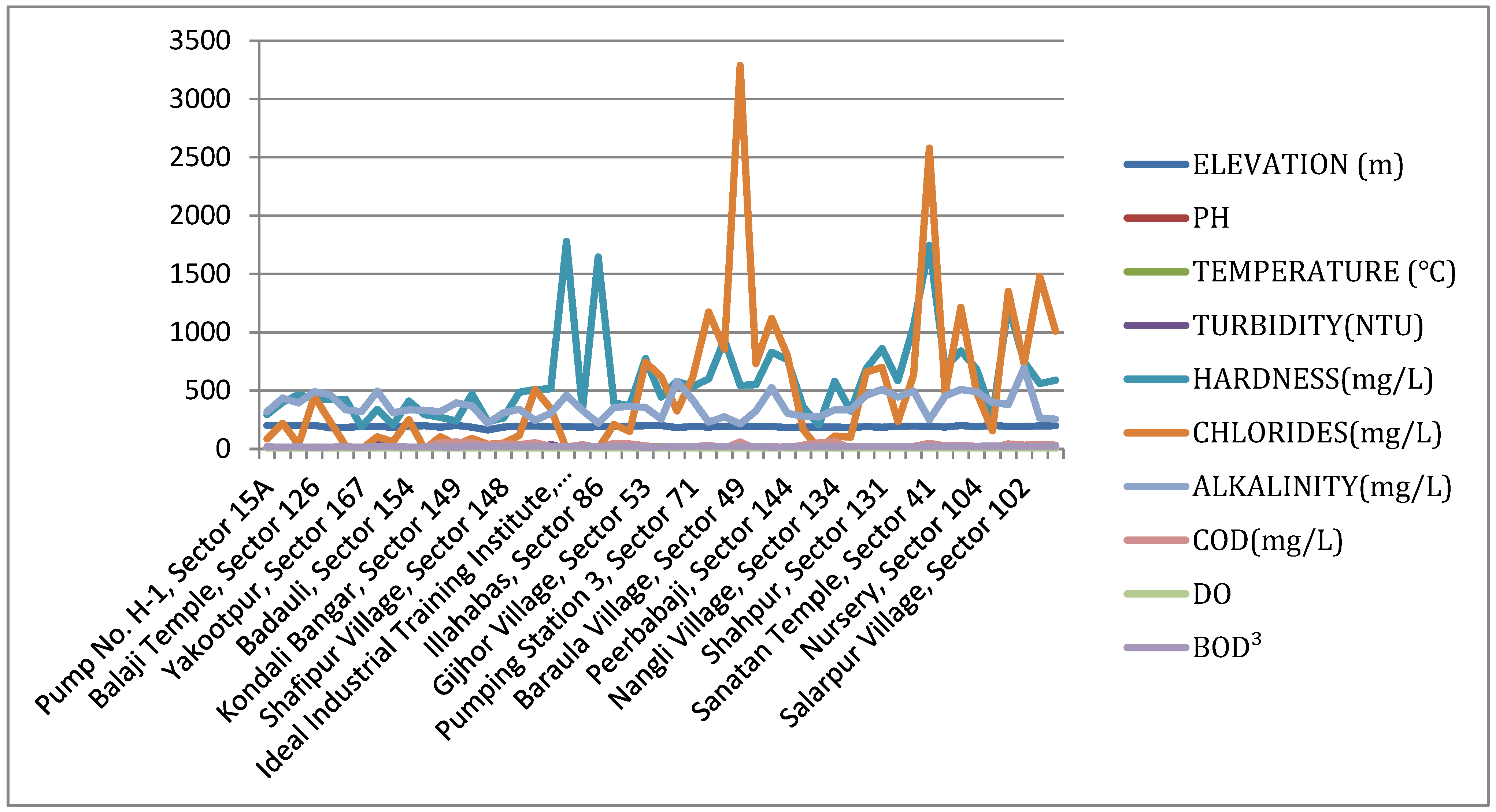
3.1. Data Acquisition

The data used in this paper have been collected by the Department of Computer Science, JSS Academy of Technical Education, Noida, by visiting different locations of Noida and some places of Delhi. One liter of water sample from each site was collected, and the coordinates and elevation were marked using GPS handsets and smart phones. The collected water samples from the water bodies were tested in the laboratories of JSS Academy of Technical Education, Noida. Different tests were then conducted to find the properties of the water sample, which were then placed in an Excel sheet for further preprocessing, and apply various machine-learning techniques. Mapping the location parameters with the water quality parameters was performed during the collection process.

Table 1. Dataset of the study and testing results of water samples collected from different locations of Noida.

Location	Latitude (N)	Longitude (E)	Elevation (m)	pH	Temperature (°C)	Turbidity (NTU)	Hardness (mg/L)	Chlorides (mg/L)	Alkalinity (mg/L)	COD (mg/L)	DO	BOD3	Acidity	Chlorine
Pump No. H-1, Sector 15A	28°34′34.7″	77°18′29.9″	203	8.74	15	9	295	84.97	319	16	6.4	18	NIL	NIL
AsagarpurJagirVilage, Sector 128	28°31′17″	77°20′58.2″	201	8.2	11.3	0	400	219.93	435	10.66	7.6	15.3	NIL	NIL
Hindustan Petroleum, Near Jaypee Hospital	28°30′20.9″	77°21′56.2″	198	8	16.2	0	465	34.98	395	10.66	6.8	18	NIL	NIL
Balaji Temple, Sector 126	28°32′11″	77°20′22.9″	202	8.35	15.5	0	430	449.86	490	10.66	8.4	14.4	NIL	NIL
Ankit Nursery, Sector 131	28°30′46.27″	77°21′09.12″	181	8.04	13.9	1	425	234.92	465	5.33	5.6	16.2	NIL	NIL
Green Beauty Farm, Sector 135	28°28′58.74″	77°22′59.48″	185	8.36	14.3	3	425	24.99	335	10.66	6.8	18	NIL	NIL
Yakootpur, Sector 167	28°28′32.94″	77°25′2.11″	192	8.68	14.6	3	190	0	320	10.66	6	15.3	NIL	NIL
Gulavali, Sector 162	28°28′5.37″	77°26′5″	193	8.2	14.3	56	340	104	495	5.33	5.6	19.8	NIL	NIL
Jhatta Village, Sector 159	28°27′52.09″	77°26′54.14″	186	8.6	14.3	4	205	59.98	310	16	5.6	19.8	NIL	NIL
Badauli, Sector 154	28°27′20.43″	77°27′39.94″	195	8.23	13.6	2	410	250	335	16	6.4	17.1	NIL	NIL
KambuxpurDerin Village, Sector 155	28°26′40.84″	77°27′19.39″	199	8.63	13.7	2	295	0	330	16	7.6	16.2	NIL	NIL
GujjarDerin, Kambuxpur, Sector 155A	28°27′0.77″	77°27′11.08″	186	8.51	13.3	3	270	104.96	320	53.33	6.4	16.2	NIL	NIL
KondaliBangar, Sector 149	28°26′17.01″	77°28′40.27″	201	8.33	13.7	3	240	34.98	395	58.66	8	14.4	NIL	NIL
GarhiSamastpur, Sector 150	28°25′46.9″	77°28′29.85″	186	8.06	14.2	5	470	89.97	370	53.33	3.2	26.1	NIL	NIL
Momnathal, Sector 150	28°36′33.69″	77°21′36.24″	163	8.90	17.4	3	235	39.98	220	32	6.4	18.9	NIL	NIL
Shafipur Village, Sector 148	28°26′51.99″	77°29′17.81″	188	7.95	18.4	17	265	49.98	310	42.6	5.6	23.4	NIL	NIL
MohiyapurVillage, Sector 163	28°28′42.06″	77°26′0.61″	196	7.57	18.1	2	485	114.96	340	37.33	5.6	21.6	NIL	NIL
Nalgadha, Sector 145	28°28′56.25″	77°26′24.5″	197	7.87	17.4	2	510	509.84	245	53.33	6.8	19.8	NIL	NIL
Ideal Industrial Training Institute, Sector 143	28°29′40.35″	77°25′31.13″	189	7.52	16.5	38	515	344.89	305	21.33	4.8	23.4	NIL	NIL
Shahdara, Sector 141	28°30′17.25″	77°25′03.87″	191	7.1	16.9	4	1780	0	460	16	6.4	23.4	NIL	NIL
Hindon Flood Plain, Kulesara, Sector 140	28°30′43.61″	77°25′47.52″	188	8.27	15.6	6	335	30	330	37.33	6.8	18	NIL	NIL
Allahabad, Sector 86	28°31′16.56″	77°24′33.91″	189	7.79	16.1	5	1645	0	220	10.66	6.8	20.7	NIL	NIL
SaiDham Colony, Sector 88	28°32′09.68″	77°25′36.11″	194	7.94	15.4	1	395	210	355	48	6.8	19.8	NIL	NIL
Kakrala Village, Sector 80	28°33′03.11″	77°24′38.26″	196	8.11	15.8	9	370	150	365	42.66	6	19.8	NIL	NIL
Gijhor Village, Sector 53	28°35′24.07″	77°21′47.86″	198	7.54	18.6	1	775	744.77	355	26.66	8.4	15.3	NIL	NIL
Sarfabad, Sector 73	28°35′20.83″	77°23′08.45″	200	8.28	17.7	1	445	619.81	255	10.66	8	17.1	NIL	NIL
Sorkha Village, Sector 118	28°34′49.64″	77°24′22.11″	183	7.67	17.8	19	580	324.9	580	21.33	6.4	18.9	NIL	NIL
Pumping Station 3, Sector 71	28°35′35.91″	77°22′33.01″	193	7.6	18.8	1	535	614.81	420	16	5.2	22.5	NIL	NIL
Pump House, Sector 122	28°35′39.79″	77°23′21.22″	187	7.65	18.1	0	600	1174.64	230	32	6	20.7	NIL	NIL
19, Block H, Sector 116	28°34′08.65″	77°23′45.80″	194	7.97	18.6	1	935	854.73	275	5.33	6	21.6	NIL	NIL
Baraula Village, Sector 49	28°33′59.25″	77°22′12.96″	194	7.54	18.7	21	545	3288.98	215	58.66	6.4	19.8	NIL	NIL
Pumping Station, Sector 35	28°34′50.46″	77°21′11.94″	193	7.83	17.5	1	550	729.77	325	0	6.8	20.7	NIL	NIL
Pumping Station 3, Sector 34	28°35′07.80″	77°21′23.59″	192	7.58	17.3	6	830	1119.65	525	21.33	8	15.3	NIL	NIL
Peerbabaji, Sector 144	28°29′26.73″	77°26′02.80″	183	8.45	17.3	20	765	799.75	305	10.66	6.8	18	NIL	NIL
Dallupura Village, Sector 164	28°28′57.49″	77°25′47.42″	189	8.65	16.6	0	360	164.95	280	32	8	17.1	NIL	NIL
Dostpur, Mangrauli, Sector 167	28°29′01.19″	77°24′57.37″	186	8.78	16.6	50	205	0	275	53.33	6.4	19.8	NIL	NIL
Nangli Village, Sector 134	28°29′52.94″	77°22′53.76″	188	8.55	16.7	0	580	109.97	335	64	7.2	18	NIL	NIL
Bakhtawarpur, Sector 127	28°32′03.14″	77°21′13.73″	185	8.31	14.1	6	325	99.97	335	5.33	6	20.7	NIL	NIL
Sultanpur Village, sector 128	28°31′17.97″	77°22′06.05″	190	7.75	16.7	0	690	659.8	460	10.66	5.6	20.7	NIL	NIL
Shahpur, Sector 131	28°30′56.37″	77°22′04.54″	186	7.91	15.1	0	860	699.78	510	16	6	19.8	NIL	NIL
Sadarpur, Sector 45	28°33′02.93″	77°21′02.22″	194	8.01	13.5	7	585	234.93	445	0	5.2	21.6	NIL	NIL
Chhalera, Sector 44	28°33′02.49″	77°21′02.57″	195	7.78	16.0	0	1055	634.8	495	21.33	7.2	16.2	NIL	NIL
Sanatan Temple, Sector 41	28°33′53.91″	77°21′36.79″	194	7.97	16.3	1	1745	2579.2	250	48	3.6	20.7	NIL	NIL
Shiv Mandir, Sector 31	28°34′37.29″	77°20′48.62″	187	7.74	16.5	0	695	479.85	455	26.66	6	21.6	NIL	NIL
NaglaCharanDass, Noida Phase-2	28°32′25.47″	77°24′25.02″	200	7.95	16.3	4	840	1214.62	510	32	6	21.6	NIL	NIL
Nursery, Sector 104	28°32′13.48″	77°21′54.55″	190	7.85	16.4	1	685	484.85	490	21.33	4.4	23.4	NIL	NIL
Pumping Station, Sector 80	28°33′15.36″	77°24′23.03″	201	8.12	17.4	0	290	154.95	400	10.66	4.4	25.2	NIL	NIL
Shiv Mandir, Sector 93	28°31′35.64″	77°22′35.64″	192	7.80	17.3	1	1230	1349.58	380	42.66	5.2	22.5	NIL	NIL
Salarpur Village, Sector 102	28°32′50.20″	77°22′56.28″	192	7.48	18.0	0	750	729.77	695	32	4.8	23.4	NIL	NIL
GarhiChaukhandi, sector 121	28°35′58.99″	77°23′41.18″	197	8.01	17.2	0	560	1479.54	265	37.33	5.2	21.6	NIL	NIL
Pumping Station, Block-G, Sector 63	28°35′58.94″	77°23′41.32″	199	7.92	17.7	0	590	1009.69	255	32	4.4	24.3	NIL	NIL

shows the snapshot of data collected from different locations in Noida and Delhi. Figure 1 presents a graphical representation of the data with different factors of the samples collected from different locations in Noida and Delhi.

The different parameters that were tested are as follows:

3.1.1. Temperature

Temperature is the physical property that expresses the coldness or hotness of water and can be further described as thermal energy measurement. Due to variance in temperature, other parameters, including chemical and physical properties, change. It broadly affects parameters including pH and oxidation as follows:

• pH: For an increase in temperature, the ratio of ionization to its molecule increases, hence increasing the toxicity of water by increasing the chemical content.
• Toxicity: A rise in temperature leads to an increase in solubility of compounds, which increases toxicity.
• Metabolic rate: It has been observed that metabolic rates of aquatic plants increase, whereas fishes such as salmon and trout decrease because they prefer colder temperatures. It does not affect the temperature but shows how metabolic rates change with the change in temperature.
• Dissolved oxygen: Increase in temperature results in an increase in solubility of oxygen and other gases. Thus, lakes and streams with lower temperatures can hold more dissolved oxygen than warmer water. As dissolved oxygen increases too much, it increases bacteria and algae, which results in contamination.

Temperature [42] plays a vital role in shaping the physical property of water as it also affects the other parameters, which leads to harm to the aquatic life of the water body.

3.1.2. pH

It is a measurement of the concentration of hydrogen ions in water, indicating the sample’s acidity. It is measured on a scale of 0 to 14, with 7 being the midpoint and is neutral, whereas a pH [42] above 7 is alkaline and becomes more alkaline as it reaches 14; a pH [43] below 7 is acidic and becomes more acidic as it reaches 0 value. pH with a value of 7; hence, non-acidic and non-alkaline is considered as perfectly drinkable water. A key water-quality metric is pH (negative base-10 logarithm of hydrogen ion activity). It is easily tested on-site, and it determines the solubility and mobility of numerous dissolved metals, as well as the sorts of gases and minerals with which groundwater has interacted as it travels from the recharge zone to the sample site. The pH of water varies due to the following factors:

• Bedrock and soil composition affect the pH as rocks such as limestone neutralize the acid, whereas rocks such as granite do not affect the pH, resulting in deviation of the pH from the required level of 7.
• Plant growth and organic material in the water body release carbon dioxide when they decompose, which combines with water forms carbonic water and converts the water to slightly acidic.
• Acid rain pollutes the water because they contain nitrogen oxides (NOx) (x could be 2 or 3 depending on if it is dioxide or trioxide) and sulfur dioxide (SO₂) along with water vapor, thus increasing the acidity of the water.
• Iron sulfide, a mineral found in and around coal, combines with water to form sulfuric acid, a strong acid; hence, coal mine drainage severely affects the pH of the water.

The pH of groundwater reacting with sandstones ranges between 6.5 and 7.5, but the pH of groundwater running through limestone strata can reach 8.5. The pH of water is essential for aquatic life and drinkability, and even a slight change in pH affects the drinkability of the water. Non-neutral water consumption is hazardous for health. Pure water has a neutral pH of 7.0 at normal temperature. The pH of rain that has balanced with atmospheric carbon dioxide is around 5.6. The pH of streams and lakes in rainy areas is usually between 6.5 and 8.0. Ground water that has come into touch with decomposing organic matter can have a pH as low as 4.0, and water that has interacted with iron sulfide minerals in coal or shale can have an even lower pH. Groundwater pH normally varies from 6.0 to 8.5 in the absence of coal or iron sulfide minerals, depending on the kind of soil and rock affected.

3.1.3. Chlorides

Chlorides [44] are salts formed due to the intermixing of metal with gaseous chlorine, and can be used to disinfect surfaces. They are present in molecules such as magnesium chloride (MgCl₂) and sodium chloride (NaCl). Content in drinking water does not cause harm, but a high amount, the sodium associated with it causes health concerns such as diarrhea. There are many sources from which chloride can enter the drinking water.

• Agricultural waste increases the chloride content in water.
• Rocks that contain chloride content.
• Waste water from wastewater treatment plants also has a high amount of chloride content in them.
• The industrial waste also contains high amounts of chloride.

High levels of it also affect aquatic lives because of the toxicity it causes. However, guidelines suggest the chloride content should be less than 250 mg/L, and more than this will make water unfit for drinking and also affect aquatic life.

3.1.4. Dissolved Oxygen

Dissolved oxygen is the oxygen dissolved [43] in water by diffusion from the surrounding air. Photosynthesis by aquatic plants and some bacteria are responsible for oxygen as it splits oxygen from the water and carbon dioxide. Phytoplanktons in oceans supply a total of three-fourths of oxygen on earth. Good water quality requires adequate dissolved oxygen, and a level below 5.0 mg/L puts aquatic life under stress and is also not fit for drinking. Biologically, the oxygen level is more important for water quality than are fecal coli form levels, and it also affects properties such as odor, clarity, and taste. It is affected by a change in temperature, such as higher temperatures.

This lowers the dissolved oxygen level of water, because as the temperature rises, the maximum level of dissolved oxygen that a water body can have, decreases, resulting in the growth of algae and bacteria in water, and hence contaminating the water body.

3.1.5. Alkalinity

Water can neutralize the acid present in the water, which is the reverse of alkalinity [45]. This occurs naturally in water due to the soil or the rocks present on the water body’s floor [46]. They are present as compounds of hydroxyl, carbonates, bicarbonates, and phosphates, silicates, etc. It has health benefits such as bone-strengthening, but high levels may lead to metabolic alkalosis, confusion, muscle twitching, etc. They also cause harm to aquatic life because they make the water alkaline, which is not be suitable for certain types of marine life to exist. The alkalinity of water must be between 20 and 200 mg/L to be considered fit for drinking purposes.

A decrease in temperature affects the alkalinity of the water body. By increasing its alkalinity, the water is made unfit for drinking.

3.1.6. Chemical Oxygen Demand (COD)

The quantity of dissolved oxygen required to oxidise chemical organic compounds such as petroleum is known as chemical oxygen demand (COD) [47]. It is used to characterize different types of water such as industrial waste, sewage, etc. It is a quality measure used to determine the amount of inactive organic and biologically active substances in a water body. The COD limit must be less than 250 mg/L to be fit to be discharged in a water body. Higher COD levels mean more oxidizable organic material to remain in water samples [48], which causes dissolved oxygen levels to drop down and, as a result, causes anaerobic conditions that are not fit for drinking nor for aquatic life to be sustained. Suppose that the COD of the water body was more than 250 mg/L, in this case, the water body would have a harmful amount of inactive, organic, and biologically active substances, making the water unfit for drinking.

3.1.7. Hardness

It is the amount of dissolved magnesium and calcium that is present in water in dissolved form. Traditionally the water can have reactions with soap [49]. Hard water is also constituted of other cations such as aluminum, iron, manganese, zinc, barium, etc. The source of the addition of these substances in water is sedimentary rocks such as chalk and limestone. Magnesium and calcium are both present in ground water [50] and running water, usually in concentrations of 100 mg/L for calcium and between negligible and 100 mg/L for magnesium. They both are essential minerals that benefit our body, but inadequate concentrations of calcium cause health issues such as kidney stones, hypertension, obesity, stroke, etc. Magnesium causes coronary heart disease, metabolic syndrome, etc. Hence, adequate amounts of these metals are needed in dietary needs. However, an excess of these can cause decreased absorption of food in the intestines due to a reaction, in the case of calcium, whereas excessive magnesium causes diarrhea [51,52]. The water with 0–17.1 mg/L of hardness is called soft water and is perfect for drinking purposes. Hard water also affects the functioning of the liver and can also result in hair loss.

3.1.8. Turbidity

The cloudiness or opaqueness of water samples is due to suspended particles such as clay-, silt-, iron-, and magnesium-like chemicals [53]. There are more if the water is more opaque, whereas there are less if the water is clear, as light is more scattered if the suspended particles are present in massive amounts, indicating that the turbidity is high. Low turbidity suggests that there are fewer pathogens present in the water. Upon consumption, high turbid water can cause endemic gastrointestinal disease, and crystal-clear water has turbidity below 1 NTU, which means drinking water must have turbidity below 1 NTU. More than the permissible limit of turbidity contaminates the water by making it unfit for human consumption and poses a danger to the aquatic life of the water body.

3.1.9. BOD (Biological Oxygen Demand)

The quantity of oxygen required to eliminate waste organic matter from water during the decomposition process by aerobic bacteria is measured by BOD (those bacteria that live only in an environment containing oxygen). The breakdown of waste organic stuff by live bacterial organisms that require oxygen to function stabilizes or renders it unobjectionable. BOD is a measure of organic contamination in water that is commonly used in wastewater treatment plants.

3.1.10. Acidity

Acidic groundwater is a serious environmental and social issue that arises as a result of changes in the ground and hydrological systems, such as the building of deep flood control channels, and wet and dry seasons. By analyzing the pH of water acidity can be found.

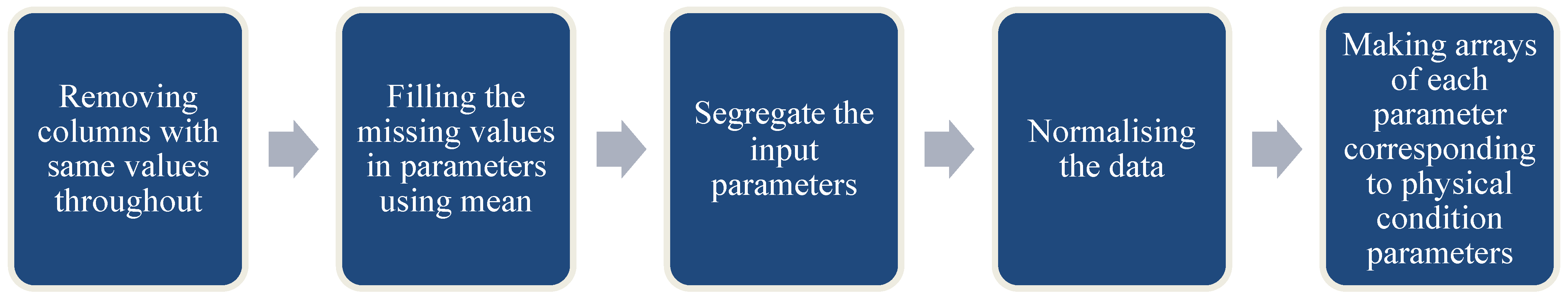
3.2. Data Pre-Processing

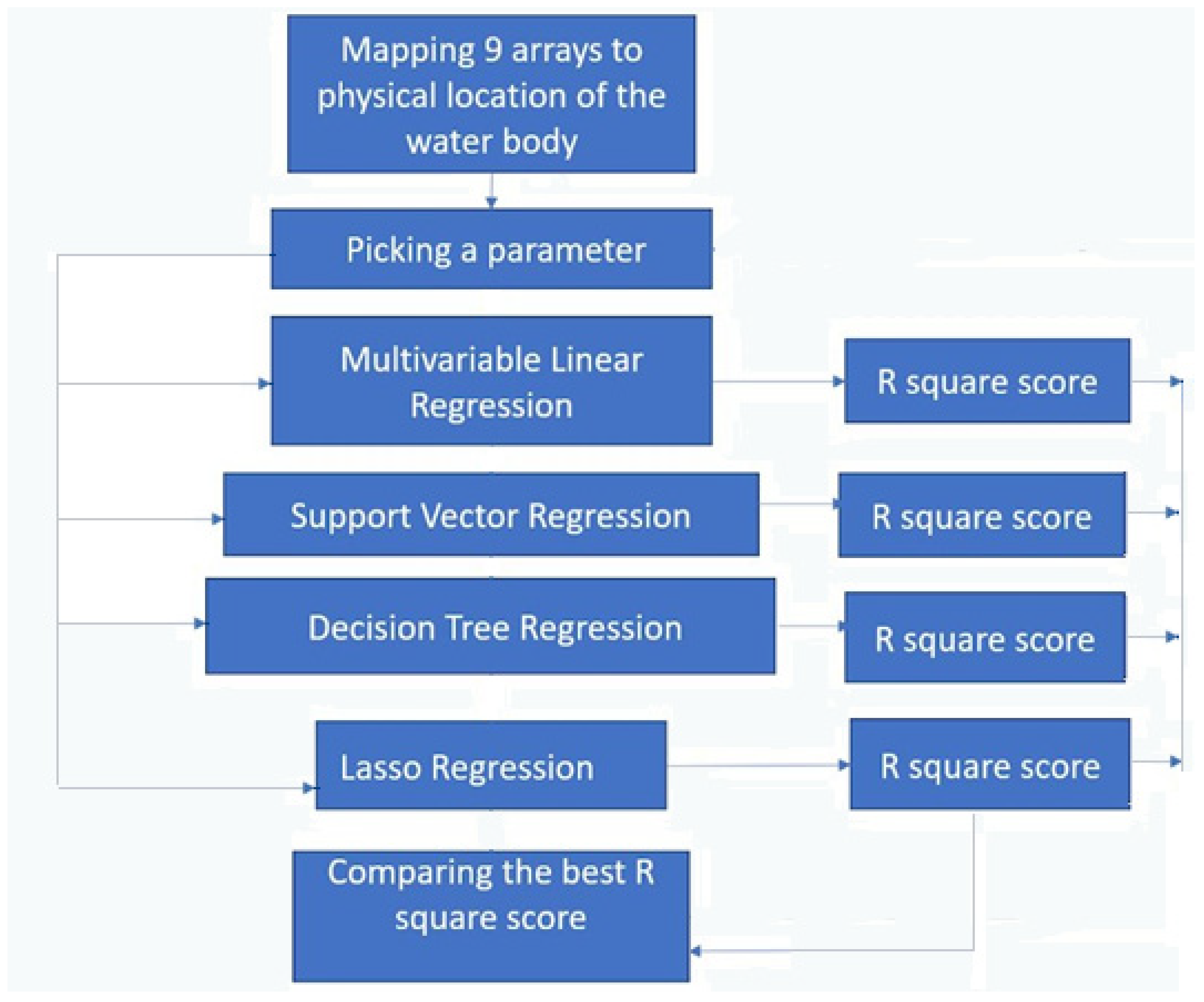
The problem encountered with the whole system was the unavailability of data at some coordinates, which was later dealt with by understanding the role of each parameter in the algorithm. The parameters were to be predicted using the present physical parameters such as latitude, longitude, and elevation. At first, the non-affecting parameters were removed where the location was removed, as they did not give us any unique number. The latitude and longitude were used instead of the location. After this, the redundant parameters that were not showing any results were also removed from the data. Different arrays were made to match the physical parameters to the changeable parameters. The number of changeable parameters was equated, keeping in account the instances of a particular parameter. Figure 2 shows the flow chart of data pre-processing.

3.3. Processing

After pre-processing, latitude, longitude, elevation were used to predict pH, temperature, turbidity, hardness, chlorides, dissolved oxygen, alkalinity, chemical oxygen demand, etc. Parameters are differentiated into physical parameters (which cannot be changed) and changeable parameters. Physical parameters were then mapped one by one to each changeable parameter in an array, which resulted in nine arrays. These nine arrays were then fed into the machine-learning models that are being used in this paper.

Four models were used while considering that the input label will consist of the latitude, longitude, and elevation. In contrast, the features consist of the parameters such as pH, temperature, turbidity, hardness, chlorides, alkalinity, dissolved oxygen, chemical oxygen demand, biological oxygen demand, etc. Then the division of data was made into the train sets and test sets.

Next, the data were fed into the Multivariable linear regression model, Support vector regression, Decision tree regression, and Lasso regression for results.

After that, R² scores were checked for each algorithm to find out the best-suited algorithm for the dataset that we could use for classifications and usage in the future. The R² score is a statistical measure to find the goodness of the fitted data (in the algorithm) [54]. It is on a scale of 0 to 1, where close to 1 signifies better fit and close to 0 indicates a bad fit, but as we have multiplied it with a factor of 100 for a better scale, the scale is now between 0 and100.

$${\mathrm{R}}^2=(1-(\mathsf{\Sigma }(y_i-f_i{)}^2-\mathsf{\Sigma }(f_i-\overline{y}\left)\right))\times 100$$

(1)

y_i = observed data that need to be predicted; f_i = output of the data corresponding to y_i; $\overline{y}$ = Mean of the observed data.

The training and test datasets were fed into all four algorithms, and then the results were fed into the R² algorithms to understand the fitness of the algorithm. Figure 3 shows the flow chart of methodology.

3.4. Algorithms Used

The data, after pre-processing, were fed into the Multivariable linear regression model, Support vector regression, Decision tree regression, and Lasso regression for results.

3.4.1. Multivariable Linear Regression

Generally, the multiple regression model is an extension to linear regression, which comprises multiple iterations of the same linear regression data [55]. This improves the accuracy of the model. Given a dataset ${\left\{y_i, x_{i1},\dots \dots , x_{ip}\right\}}_{i=1}^n$ of n statistical sites, a linear regression model will assume the yi based on the factors x.

y = β₀ + β_1×1 + β_2×2 + … + β_k×k + ∈

(2)

where ∈ is error, β_i are slope constants, and y and x_i are output and input variables.

This algorithm is fed with the training dataset such that the input x is fir in the Equation (2), which then makes a random value of the β_i and maps it with the actual y. This process keeps iterating up to multiple times until the set of β_i is not found with the least possible error. Those β_i are then placed in Equation (2) to predict the output y. We can map the parameters using this algorithm.

3.4.2. Support Vector Regression

This is the most common regression technique for the classification of a water-based regression model. It is well known for its accuracy, and the nature of classification is simple. The procedure involves making a hyper plane that exists between the classes; it maximizes the distinction by making a significant difference in the parameter assignment. These results in low mismatch ratios. Training of the SVR performed by solving [56]:

$$\mathrm{minimize}\frac{1}{2}{\Vert w\Vert }^2$$

(3)

$$\mathrm{subject}\mathrm{to}|y_i-\langle w,x_i\rangle -b\le \epsilon$$

(4)

$$y=wx+b$$

(5)

where x_i is a training sample with a target yi. $\langle w,x_i\rangle +b$ is the prediction for the sample. ϵ is a free parameter that serves as a threshold that all the predictions have to be within an ϵ range of the accurate prediction.

In this, we feed the x_i to the Equation (4) such that the Equation (3) is minimized, and after finding the suitable w, it is then provided to the equation of the hyper plane (5). The result of the hyper plane equation is the predicted value of y, which is afterward used in R² score. We can map the parameters using this algorithm.

3.4.3. Decision Tree Regression

Decision trees construct regression or arrangement models as a tree structure [57]. It divides a dataset into primary subsets while simultaneously a related decision tree is steadily evolved. The conclusive outcome is a tree with decision hubs and leaf hubs. This algorithm is used for both classification and regression. It is the regression model that uses entropy to select as the main parameter within the variables. After this, it makes a top to bottom line tree to determine all the decisions in the classification regression tree.

A decision tree is constructed top-down from a root hub and includes dividing the information into subsets that contain occurrences with comparable qualities (homogenous). In this, it utilizes standard deviation to ascertain the homogeneity of a numerical example. In the event that the numerical model is totally homogeneous, its standard deviation is zero.

Gini index = 1 − Σp²

(6)

p_i is the probability of happening of event p_i.

In this, the predicted outcome is a real number and not a class. In the process of making the tree, the data need to be classified level-wise, which is performed by using the concept of Gini impurity or Information gain. The objective is to figure out the minor Gini impurity feature as the root node, giving us a better solution. To compute the Gini impurity for class Items set, once the data are fed into it, it will make a decision tree based on the entropies of the probability of each. It will then decide the following most probable answer based on the regression of the data.

3.4.4. Lasso Regression

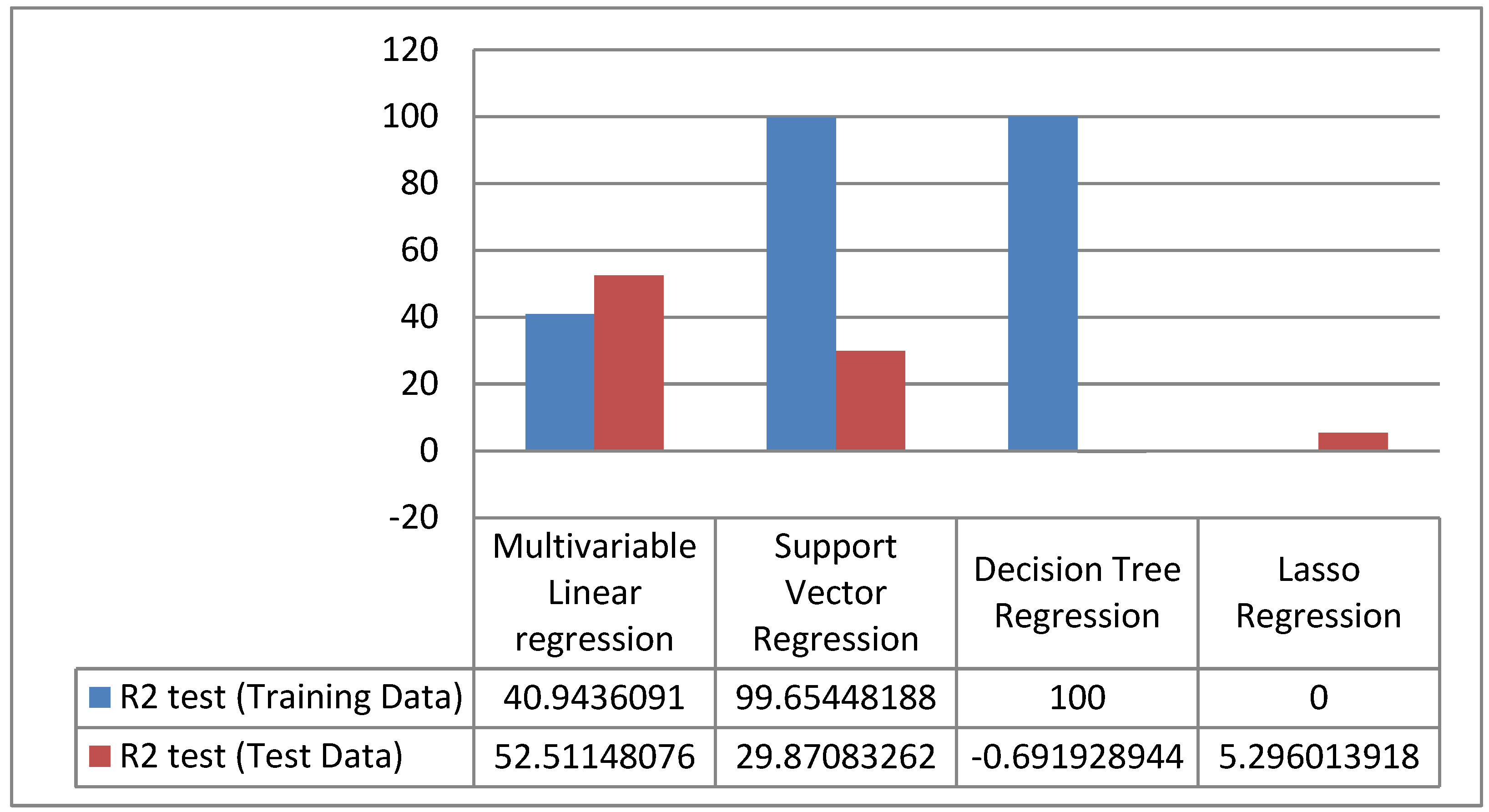
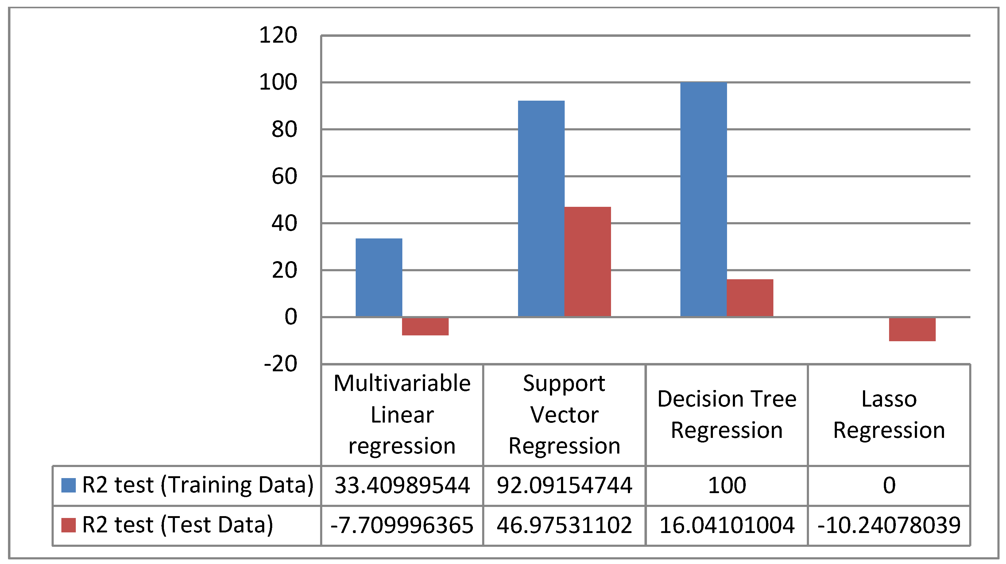
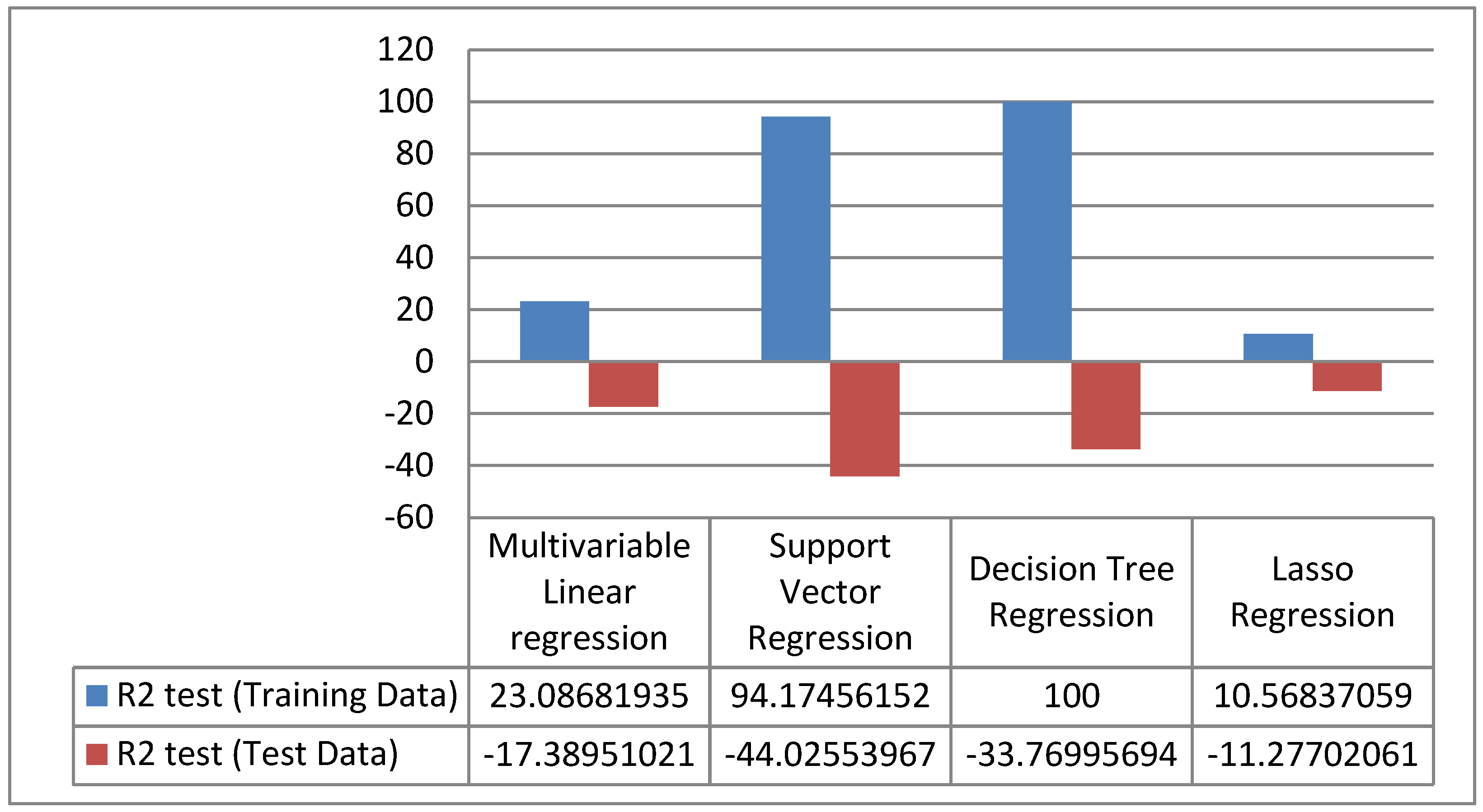
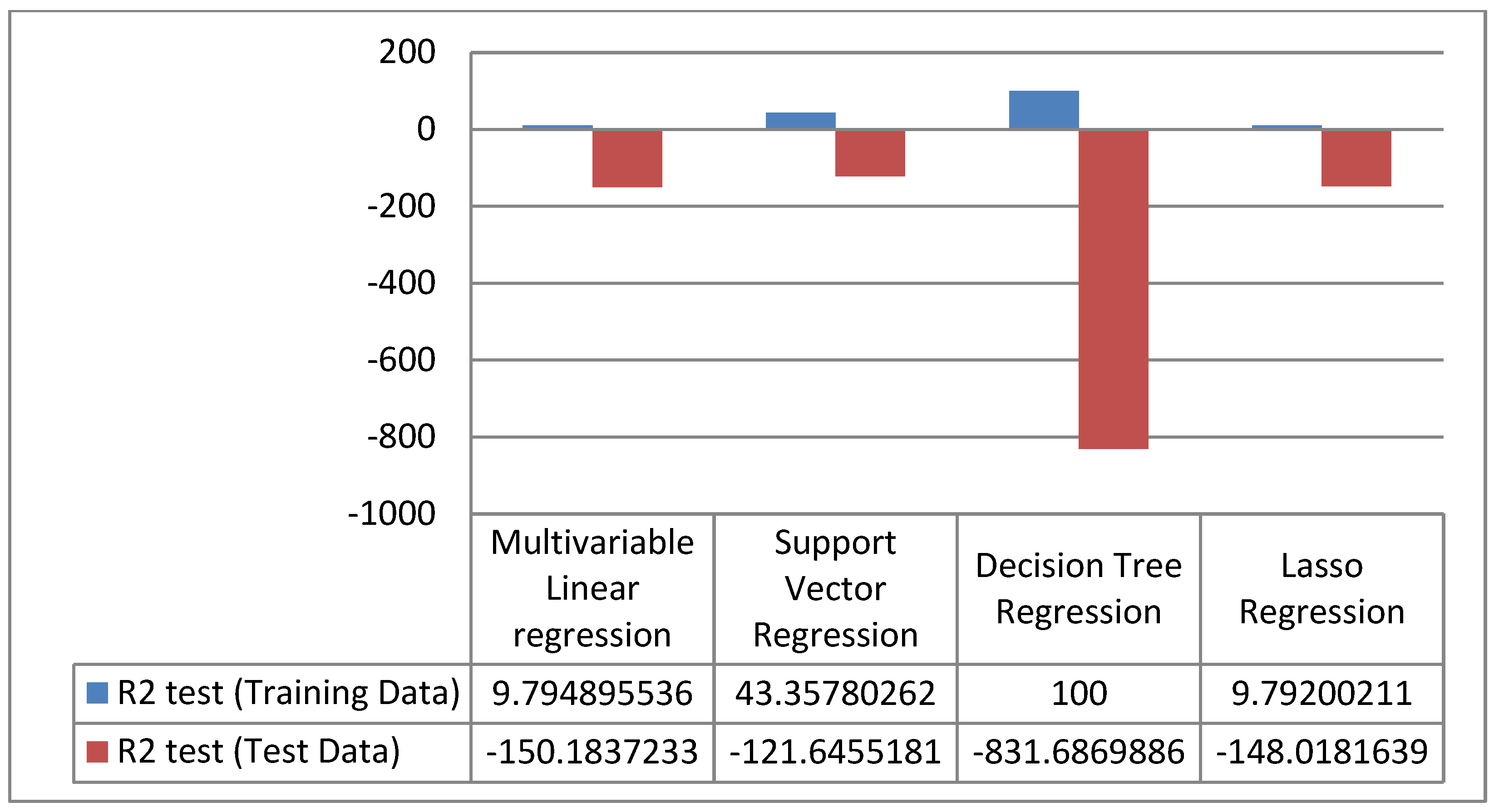
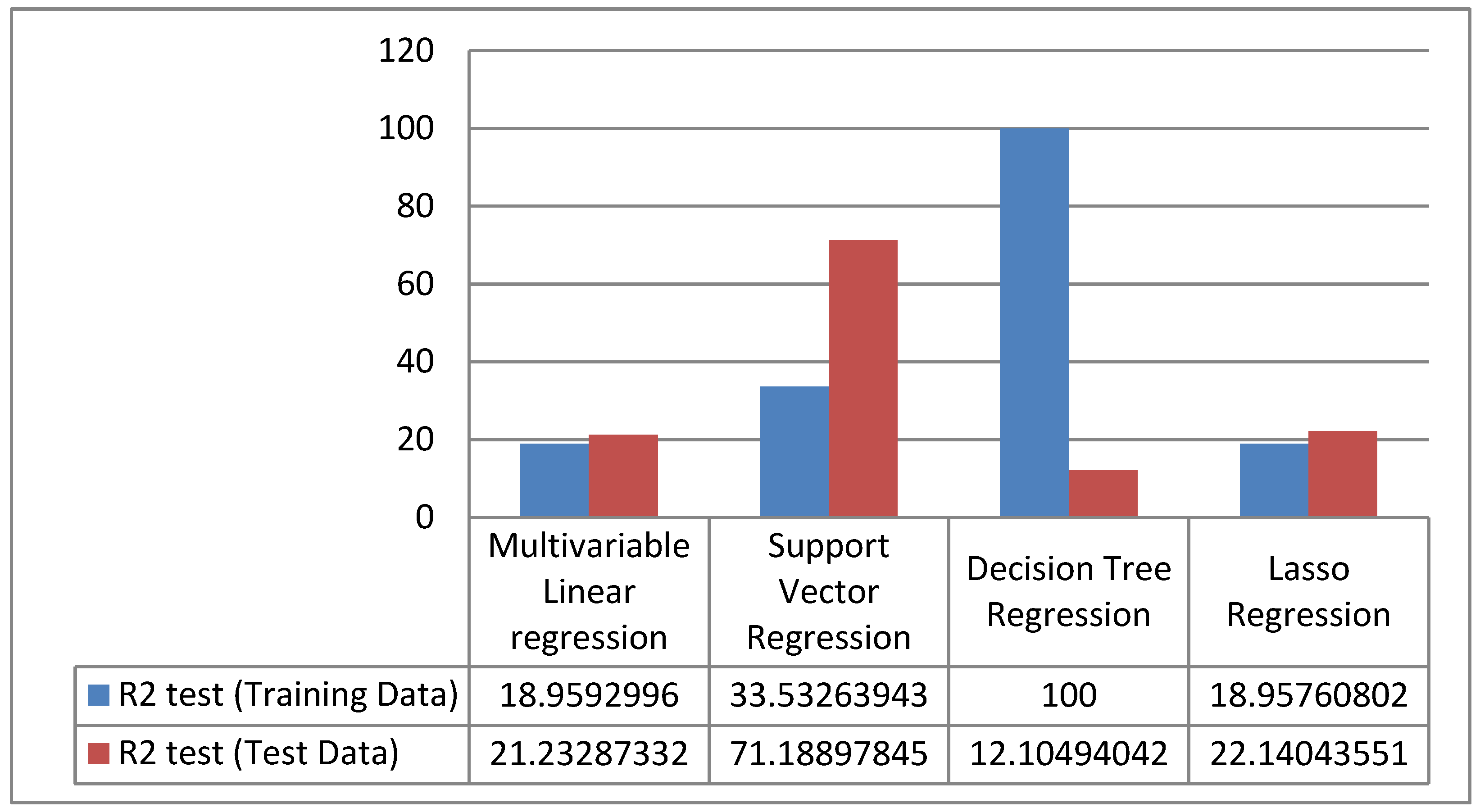
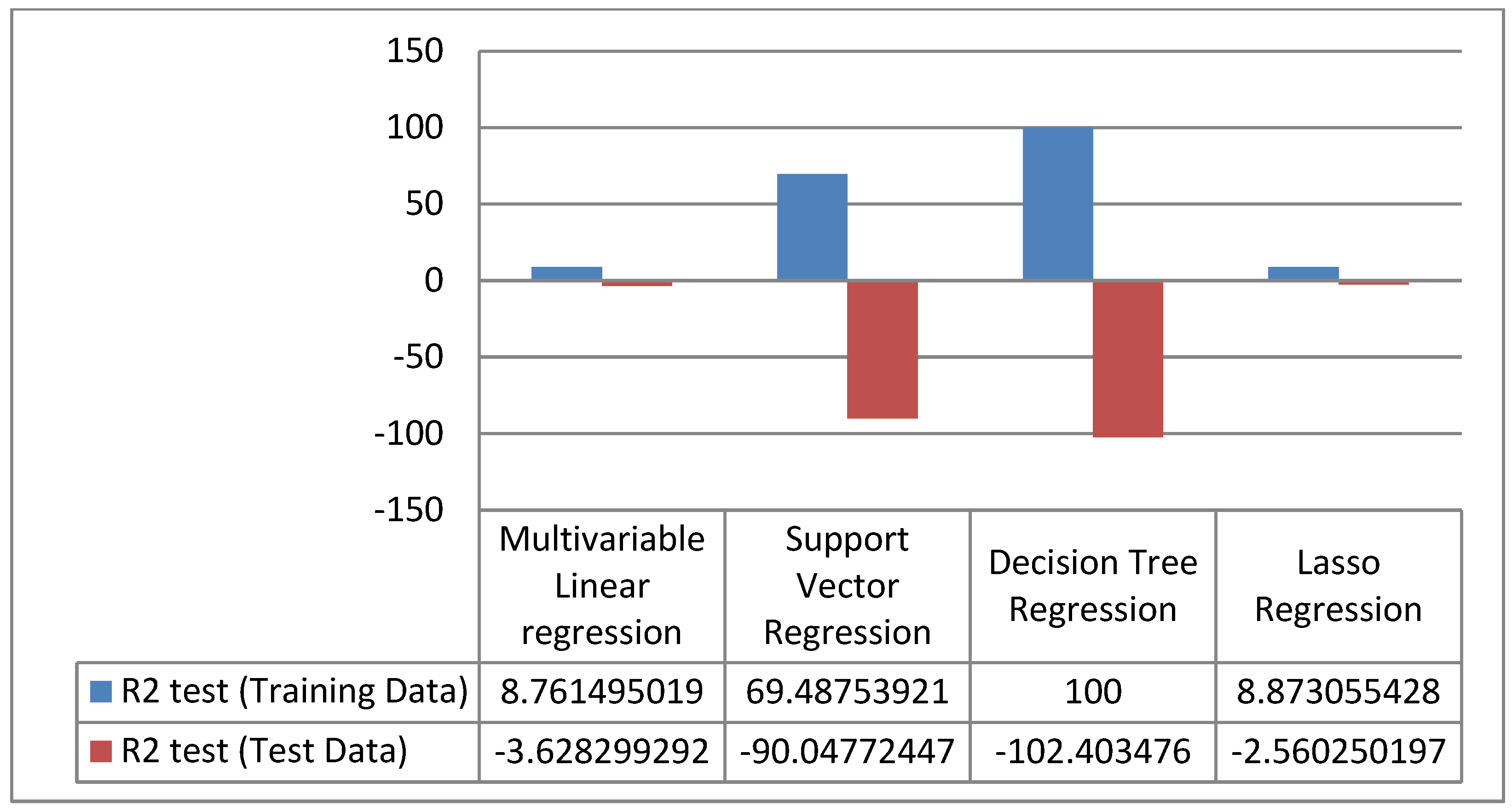
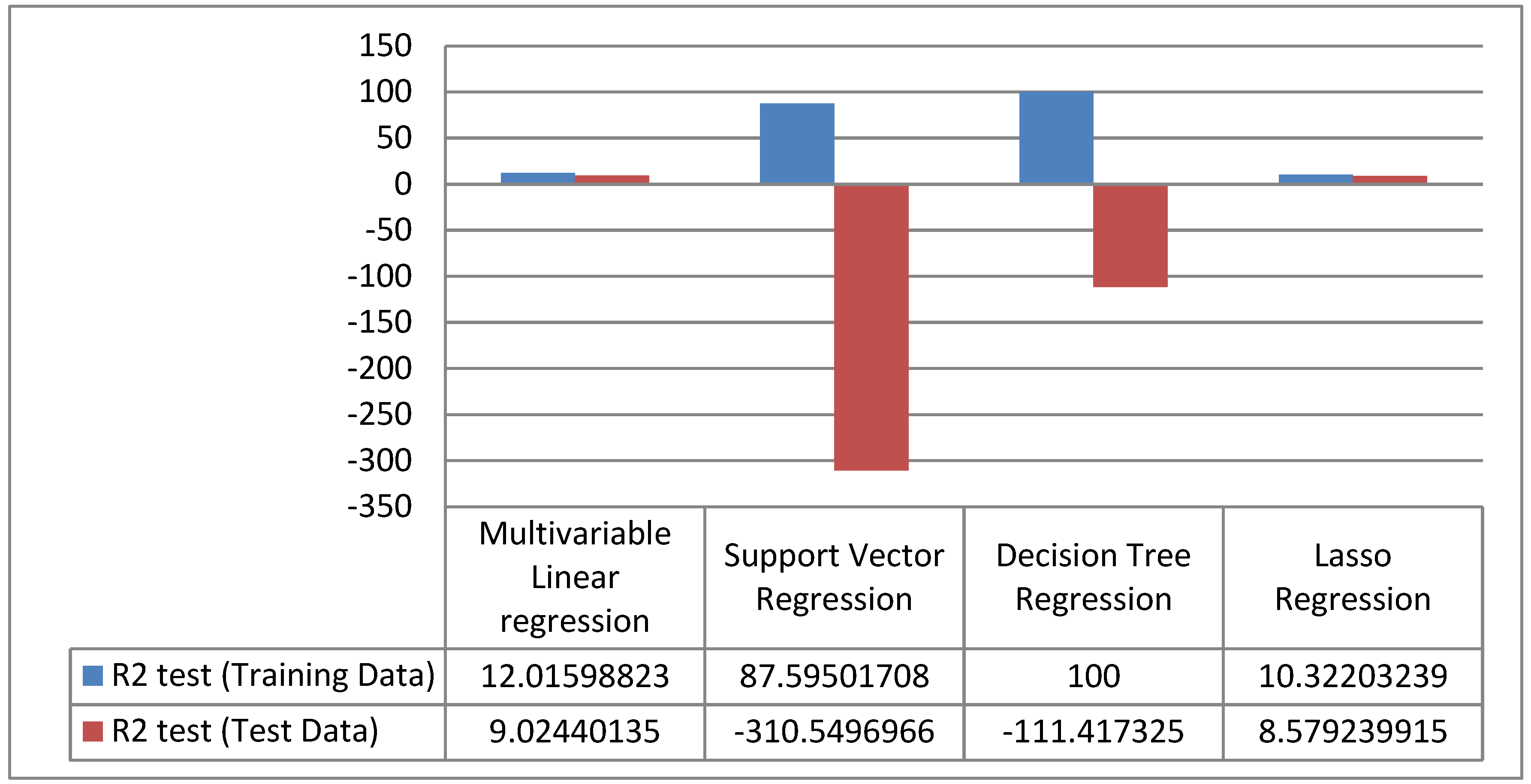
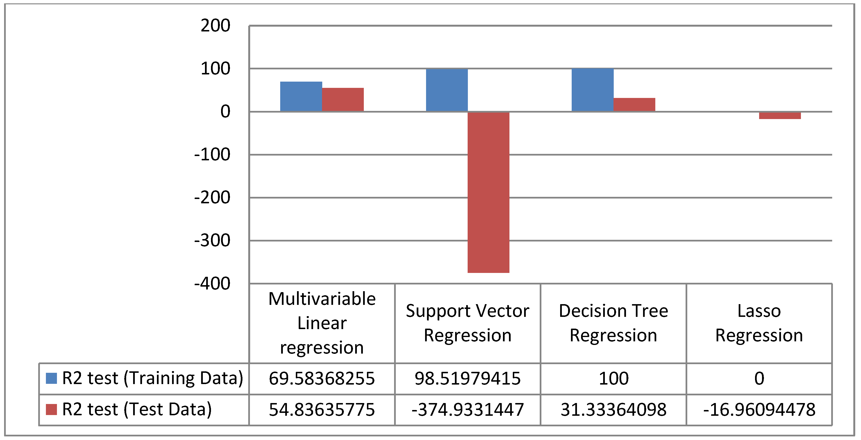
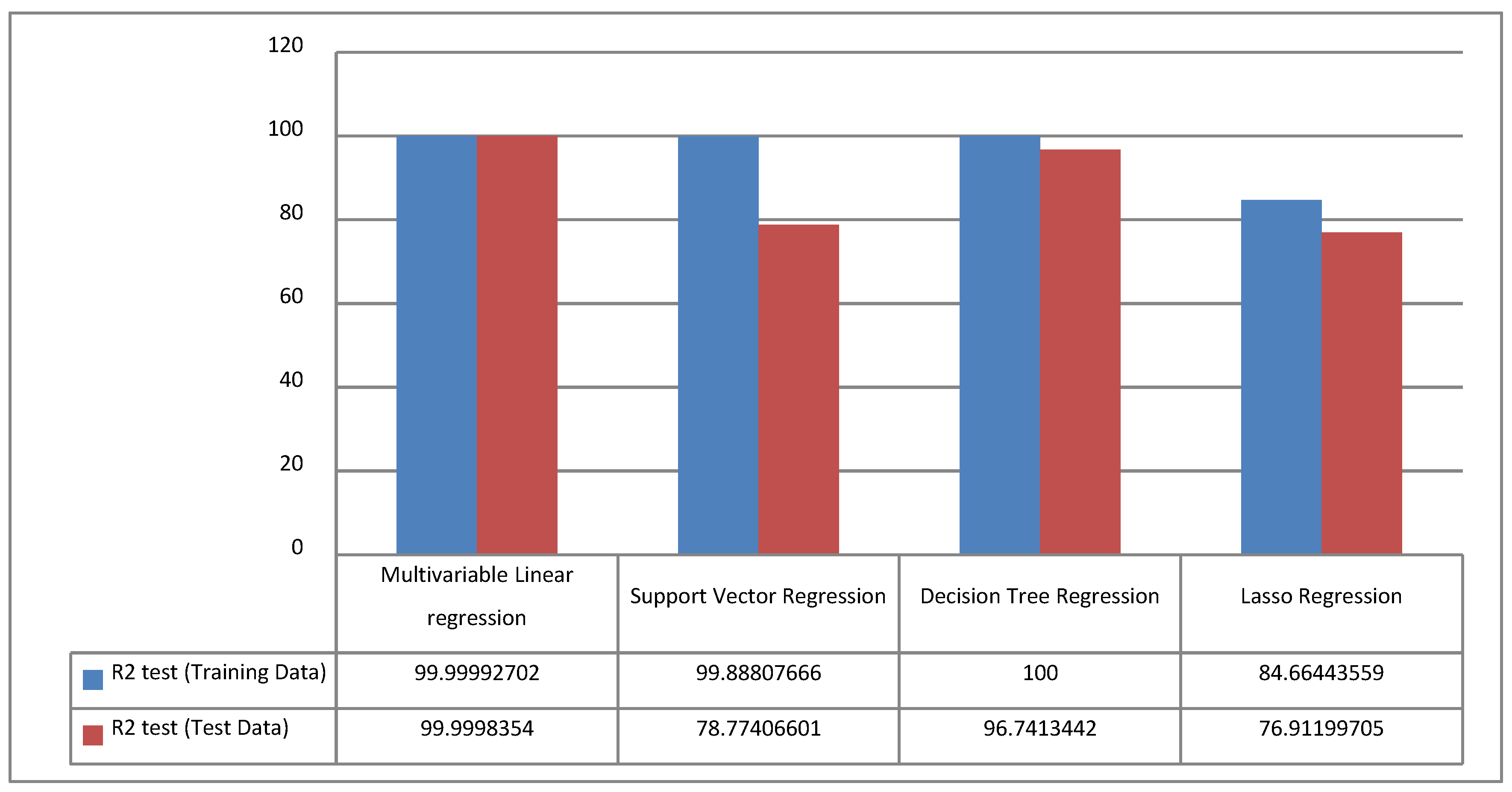
Lasso (least absolute shrinkage and selection operator) is a regression analysis method that performs variable selection and regularization to improve the prediction accuracy [58]. Lasso regression is a sort of linear regression that utilizes shrinkage. Shrinkage is the place information esteems are contracted towards an essential issue, similar to the mean. The lasso methodology empowers straightforward, meager models (for example, models with fewer parameters). This specific sort of regression is appropriate for models indicating significant levels of multicollinearity or when you need to robotize certain pieces of model choice, similar to variable determination/parameter enhancement. For lasso, this equation needs to be solved:

$$\begin{array}{c}min\\ {\beta }_o,\beta \end{array}\left\{{\displaystyle \sum }_{i=1}^N\left(y_i-{\beta }_o-x_i^T\beta \right){ }^2\right\}\mathrm{subject}\mathrm{to}{\displaystyle \sum }_{j=1}^p\left|{\beta }_j\right|\le t$$

(7)

where ${\Vert \beta \Vert }_p={\left({\displaystyle \sum }_{i=1}^N{\left|{\beta }_i\right|}^p\right)}^{1/p}$ is the standard L^p norm, and 1N is N × 1 vector of ones? t is a specified parameter that determines the regularization amount.

When data are fed into the regression algorithm, it works like linear regression by using random parameters, shrinking the cost function, and using those coefficients in the equation. The cost function that decides the parameters is the least for best coefficients in the equation. The results in lasso regression are then used to find its R² scores, which then determine the following most probable answer based on the regression of the data.

4. Results

After collecting the results of the tested samples, the properties of water as parameters were found and were ready to be used for machine-learning algorithms. It was observed that machine learning could be used to find the contaminating parameters using the physical parameters as input parameters. Since the physical parameters are non-changeable for a location, they were mapped with the changeable parameters to yield output and predict the contaminating factors. So, after implementing four regressions on the dataset, we obtained the results that helped us conclude that Multivariable linear regression works the best in most cases. As we increase the instance count in the dataset, the results start to improve even further. The current effects on those parameters are:

Figure 4 shows the R² results for temperature. From this, we can conclude that Multivariable linear regression showed the best results.

Figure 5 shows the R² results for pH. From this, we can conclude that Support vector regression showed the best results.

Figure 6 shows the R² results for turbidity, which we were unable to conclude because of less correlation among the data.

Figure 7 shows the R² results for the hardness of the water, which we were unable to conclude because of less correlation among the data.

Figure 8 shows the R² results for Chlorides. From this, we can conclude that Support vector regression showed the best results.

Figure 9 shows the R² results for alkalinity, which we were unable to conclude because of less correlation among the data.

Figure 10 shows the R² results for COD. From this, we can conclude that Multivariable linear regression showed the best results, and it will improve as the dataset size increases.

Figure 11 shows the R² results for DO. From this, we can conclude that Multivariable linear regression showed the best results, and it will improve as the dataset size increases.

Figure 12 shows the R² results for BOD. From this, we can conclude that Multivariable Linear regression showed the best results, and it will improve as the dataset size increases.

The statistical analysis of the data was performed after splitting them into two parts, namely, training data and test data. Thus, they show different results on each parameter and model. The data were divided into 80% for training part, and 20% is the test part, and all of them showed their respective R² scores.

5. Discussion

The main aim of this research was to create a relationship between the location-based factors with the factors affecting the water contamination in a given area. Some research has been conducted in the past where water contamination has been found in an area for a given time line, but no study was available where water contaminants are predicted using the location coordinates. In simple words, it can be stated that if we have the data of n locations in a particular area, this study can help to predict the water contaminants of the (n + 1)th location without physically testing the water sample of that location.

The research started with water samples collection from different locations in Noida and few in Delhi. The samples so collected were tested in the lab for finding out the different attributes of the water sample. These data were unique and had never been collected, analyzed, or used for any past study. The studies that had been carried out till now had not gone into the micro level. Moreover, in previous research, samples of all locations were collected over a time period, which makes our approach completely different, meaning that we did not collect samples for each and every location. If we had the data for n locations, we could predict the water contamination of (n + 1)th location.

This research aimed to find water factors of the contamination using a machine-learning approach where the physical parameters were used in algorithms to predict the contamination. These physical factors were mapped with each contaminating factor such that the input of the physical factor would predict one contaminating factor. R² scores for temperature in Multivariable linear regression training was 40.94, and testing was 52.51; in Support vector regression training was 99.65 and testing was 29.87; in Decision tree regression training was 100.0 and testing was −0.69; and in Lasso regression training was 0.0 and testing was 5.29. So, from this, we can conclude that Multivariable linear regression showed the best results.

R² scores for pH in Multivariable linear regression training was 33.40, and testing was −7.70; in Support vector regression training was 92.09 and testing was 46.97; in Decision tree regression training was 100.0 and testing was 16.04; and in Lasso regression training was 0.0 and testing was −10.24. So, from this, we can conclude that Support vector regression showed the best results.

R² scores for turbidity in Multivariable linear regression training was 23.08,and testing was −17.38; in Support vector regression training was 94.17andtesting was −44.02; in Decision tree regression training was 100.0 and testing was −33.76; and in Lasso regression training was 10.56 and testing was −11.27. So, from this, we were unable to conclude because of less correlation among the data.

R² scores for hardness in Multivariable linear regression training was 9.79, and testing was −150.18; in Support vector regression training was 43.35 and testing was −121.64; in Decision tree regression training was 100.0 and testing was −831.68; and in Lasso regression training was 9.79 and testing was −148.01. So, from this, we were unable to conclude because of less correlation among the data.

R² scores for chlorides in Multivariable linear regression training was 18.95, and testing was 21.23; in Support vector regression training was 33.53 and testing was 71.188; in Decision tree regression training was 100.0 and testing was 12.10; and in Lasso regression training was 18.95 and testing was 22.14. So, from this, we can conclude that Support vector regression showed the best results.

R² scores for alkalinity in Multivariable linear regression training was 8.76, and testing was −3.62; in Support vector regression training was 69.48 and testing was −90.04; in Decision tree regression training was 100.0 and testing was −111.41; and in Lasso regression training was 10.32 and testing was −2.56. So, from this, we were unable to conclude because of less correlation among the data.

R² scores for chemical oxygen demand in Multivariable linear regression training was 12.01, and testing was 9.02; in Support vector regression training was 87.59501708185957 and testing was −310.54; in Decision tree regression training was 100.0 and testing was −0.69; and in Lasso regression training was 0.0 and testing was 8.579239914991078. So, from this, we can conclude that Multivariable linear regression showed the best results and will improve as the dataset size increases.

R² scores for dissolved oxygen in Multivariable linear regression training was 69.58, and testing was 54.83; in Support Vector Regression training was 98.51 and testing was −374.93; in Decision tree regression training was 100.0 and testing was 31.33; and in Lasso regression training was 0.0 and testing was −16.96. So, from this, we can conclude that Multivariable linear regression showed the best results and will improve as the dataset size increases.

R² scores for biological oxygen demand in Multivariable linear regression training was 99.99, and testing was 99.99, in Support vector regression training was 99.88 and testing was 78.77; in Decision tree regression training was 100.0 and testing was 96.74; and in Lasso regression training was 84.66 and testing was 76.91. So, from this, we can conclude that Multivariable linear regression showed the best results and will improve as the dataset size increases.

6. Conclusions

The dataset used in this paper was collected through ground survey and analyzed through lab testing. This paper not only aimed at predicting water contamination using location coordinates, but also proposed a new method for predicting the water contamination level of a particular area. To forecast the pH, temperature, turbidity, hardness, chlorides, alkalinity, COD, DO, and BOD in groundwater, regression models (such as MVLR, SVR, DTR, and LR models) were created.

pH, temperature, turbidity, hardness, chlorides, dissolved oxygen, alkalinity, chemical oxygen demand, and other parameters were predicted using latitude, longitude, and elevation after pre-processing. Physical parameters (which cannot be modified) and changeable parameters were the two types of parameters used. After that, physical parameters were mapped one by one to each changeable parameter in an array, yielding a total of nine arrays. These nine arrays were then loaded into the machine-learning models employed in this study.

Four models were used, with the input label consisting of latitude, longitude, and elevation. The features consisted of pH, temperature, turbidity, hardness, chlorides, alkalinity, dissolved oxygen, chemical oxygen demand, and biological oxygen demand, among other factors. The data were then divided into train sets and test sets.

The data were then sent into the Multivariable linear regression model, Support vector regression model, Decision tree regression model, and Lasso regression model for analysis.

The suggested technique, which uses the regression models, has provided valuable data that decisionmakers can utilize to help manage reservoir water quality. Instead of forecasting, we focused on water quality prediction in this study. Different lead-time forecasts in water quality can be produced in future research to aid local authorities with water quality management. Soft computing approaches, such as the merging fuzzy optimum model with genetic programming, support vector machine, and the particle swarm optimization training algorithm for a neural network, can enhance reservoir water quality prediction.

References

1. Krishnan, K.S.D. Multiple Linear Regression-Based Water Quality Parameter Modeling to Detect Hexavalent Chromium in Drinking Water. In Proceedings of the 2017 International Conference on Wireless Communications, Signal Processing and Networking (WiSPNET), Chennai, India, 22–24 March 2017; IEEE: Piscataway, NJ, USA, 2017; pp. 2434–2439. [Google Scholar]
2. Aho, M.I.; Akpen, G.D.; Ekwule, O.R. Predictive regression models of water quality parameters for river Amba in Nasarawa State, Nigeria. Intl. J. Innov. Eng. Sci. Res. 2018, 2, 24–33. [Google Scholar]
3. Ahmed, U.; Mumtaz, R.; Anwar, H.; Shah, A.A.; Irfan, R.; García-Nieto, J. Efficient Water Quality Prediction Using Supervised Machine Learning. Water 2019, 11, 2210. [Google Scholar] [CrossRef] [Green Version]
4. Shrestha, A.K. The Correlation and Regression Analysis of Physicochemical Parameters of River Water fortheEvaluationofPercentageContributiontoElectricalConductivity, Hindawi. J. Chem. 2018, 2018, 8369613. [Google Scholar] [CrossRef]
5. Daud, M.K. Drinking water quality status and contamination in Pakistan. BioMedRes 2017, 2017, 7908183. [Google Scholar] [CrossRef]
6. Shafi, U. Surface Water Pollution Detection using Internet of Things. In Proceedings of the 15th International Conference on Smart Cities:Improving Quality of Life Using ICT &IoT(HONET-ICT), Islamabad, Pakistan, 2 August 2019; pp. 92–96. [Google Scholar]
7. Pant, R.R. Spatiotemporal variations of hydrogeochemistry and its controlling factors in the Gandaki river basin, Central Himalaya Nepal. Sci. Total. Environ. 2018, 622–623, 770–782. [Google Scholar] [CrossRef]
8. Khatunm, M. Phytoplankton assemblage with relation to water quality in Turag River of Bangladesh. Casp. J. Environ. Sci. 2020, 18, 31–45. [Google Scholar]
9. Rose-Rodrígue, R. Water and fertilizers use efficiency in two hydroponic systems for tomato production. Hortic. Bras. 2020, 38, 47–52. [Google Scholar] [CrossRef]
10. Trombadore, O. Effective Data Convergence, Mapping, and Pollution Categorization of Ghats at Ganga River Front in Varanasi; Springer: Berlin/Heidelberg, Germany, 2020; Volume 27, pp. 15912–15924. [Google Scholar]
11. Bapa, G. Evaluation of Physico-chemical characters of Singhia and Budhi rivers in Sunsari and Morang industrial corridor, Nepal. Int. J. Adv. Res. Biol. Sci. 2014, 1, 104–112. [Google Scholar]
12. Paudyal, R.; Kang, S.; Sharma, C.; Tripathee, L.; Sillanpää, M. Variations of the Physicochemical Parameters and Metal Levels and Their Risk Assessment in Urbanized Bagmati River, Kathmandu, Nepal. J. Chem. 2016, 2016, 1–13. [Google Scholar] [CrossRef]
13. Tripathi, B. Studies on the physicochemical parameters and correlation coefficient of the river Ganga at Holy Place, Allahabad. J. Environ. Sci. Toxicol. Food Technol. 2014, 8, 29–36. [Google Scholar]
14. Banerjee, K.; Prasad, R.A. Reference based inter chromosomal similarity based DNA sequence compression algorithm. In Proceedings of the 2017 International Conference on Computing, Communication and Automation (ICCCA), Greater Noida, India, 5–6 May 2017; pp. 234–238. [Google Scholar]
15. Banerjee, K.; Bali, V. Design and Development of Bioinformatics Feature Based DNA Sequence Data Compression Algorithm. EAI Endorsed Trans. Pervasive Health Technol. 2020, 19, 5. [Google Scholar] [CrossRef] [Green Version]
16. Banerjee, K.; Prasad, R.A. A new technique in reference based DNA sequence compression algorithm: Enabling partial decompression. In Proceedings of the AIP Conference Proceedings American Institute of Physics, Roorkee, India, 17 February 2015. [Google Scholar]
17. Yadav, N.; Banerjee, K.; Bali, V. A Survey on Fatigue Detection of Workers Using Machine Learning. Int. J. E-Health Med. Commun. 2020, 11, 1–8. [Google Scholar] [CrossRef]
18. Iwendi, C.; Maddikunta, P.K.R.; Gadekallu, T.R.; Lakshmanna, K.; Bashir, A.K.; Piran, M.J. A metaheuristic optimization approach for energy efficiency in the IoT networks. Softw. Pract. Exp. 2020, 51, 2558–2571. [Google Scholar] [CrossRef]
19. Patel, H.; Singh Rajput, D.; Thippa Reddy, G.; Iwendi, C.; Kashif Bashir, A.; Jo, O. A review on classification of imbalanced data for wireless sensor networks. Int. J. Distrib. Sens. Netw. 2020, 16, 1550147720916404. [Google Scholar] [CrossRef]
20. Iwendi, C.; Khan, S.; Anajemba, J.H.; Bashir, A.K.; Noor, F. Realizing an efficientIoMT-assisted patient diet recommendation system through machine learning model. IEEE Access 2020, 8, 28462–28474. [Google Scholar] [CrossRef]
21. Iwendi, C.; Jalil, Z.; Javed, A.R.; Reddy, T.; Kaluri, R.; Srivastava, G.; Jo, O. Keysplitwatermark: Zero watermarking algorithm for software protection against cyber-attacks. IEEE Access 2020, 8, 72650–72660. [Google Scholar] [CrossRef]
22. Iwendi, C.; Bashir, A.K.; Peshkar, A.; Sujatha, R.; Chatterjee, J.M.; Pasupuleti, S.; Jo, O. COVID-19 patient health prediction using boosted random forest algorithm. Front. Public Health 2020, 8, 357. [Google Scholar] [CrossRef]
23. Banerjee, K.; Kumar, S.; Tilak, L.N.; Vashistha, S. Analysis of Groundwater Quality Using GIS-Based Water Quality Index in Noida, GautamBuddh Nagar, Uttar Pradesh (UP), India. In Applications of Artificial Intelligence and Machine Learning; Springer: Berlin/Heidelberg, Germany, 2021; pp. 171–187. [Google Scholar]
24. Banerjee, K.; Kumar, M.S.; Tilak, L.N. Delineation of Potential Groundwater Zones using Analytical Hierarchy Process (AHP) for GauthamBuddh Nagar District, Uttar Pradesh, India; Materials Today: Amsterdam, The Netherlands, 2021; Volume 44, pp. 4976–4983. [Google Scholar]
25. Kumar, N.; Mishra, B.; Bali, V. A novel approach for blast-induced fly rock prediction based on particle swarm optimization and artificial neural network. In Proceedings of the International Conference on Recent Advancement on Computer and Communication, Paris, France, 22–23 June 2018; Springer: Berlin/Heidelberg, Germany, 2018; pp. 19–27. [Google Scholar]
26. Malhotra, S.; Bali, V.; Paliwal, K.K. Genetic programming and K-nearest neighbour classifier based intrusion detection model. In Proceedings of the 2017 7th International Conference on Cloud Computing, Data Science & Engineering–Confluence, Noida, India, 12–13 January 2017; pp. 42–46. [Google Scholar] [CrossRef]
27. Frank, J. Public Drinking Water Contamination and Birth Outcomes. Am. J. Epidemiol. 1995, 141, 850–862. [Google Scholar]
28. Osmani, S.A. An Integrated Approach of Machine Algorithms with Multi-Objective Optimization in Performance Analysis of Event Detection; Springer: Warsaw, Poland, 2020. [Google Scholar]
29. Hart, B.W. Sensor Placement in Municipal Water Networks with Temporal Integer Programming Models. J. Water Resour. Plan. Manag. 2006, 132, 1943–5452. [Google Scholar]
30. Blackburn, B.G. Surveillance for Waterborne-Disease Outbreaks Associated with Drinking Water–United States, 2001–2002; Division of Healthcare Quality Promotion, National Center for Infectious Diseases, CDC: Singapore, 2004; pp. 23–45.
31. Brunkard, J.M. Surveillance for Waterborne Disease Outbreaks Associated with Drinking Water–United States, 2007–2008; Division of Healthcare Quality Promotion, National Center for Infectious Diseases, CDC: Singapore, 2011; pp. 38–68.
32. CANARY, Sandia National Laboratoris. Available online: https://software.sandia.gov/trac/canary (accessed on 21 January 2022).
33. Deb, K. A Fast and Elitist Multi-objective Genetic Algorithm. IEEE Trans. Evol. Comput. 2002, 6, 182–197. [Google Scholar] [CrossRef] [Green Version]
34. Cristo, C. Pollution Source Identification of Accidental Contamination in Water Distribution Networks. J. Water Resour. Plan. Manag. 2008, 134, 1943–5452. [Google Scholar] [CrossRef]
35. Hasan, J.; States, S.; Deininger, R. Safeguarding the Security of Public Water Supplies Using Early Warning Systems: A Brief Review. J. Contemp. Water Res. Educ. 2009, 129, 27–33. [Google Scholar] [CrossRef] [Green Version]
36. Smitha, K. Contaminant classification using cosine distances based on multiple conventional sensors. Environ. Sci. Process. Impacts 2015, 17, 581. [Google Scholar]
37. Liu, S.; Che, H.; Smith, K.; Chen, L. Contamination event detection using multiple types of conventional water quality sensors in source water. Environ. Sci. Process. Impacts 2014, 16, 2028–2038. [Google Scholar] [CrossRef]
38. Liu, S.; Butler, D.; Memon, F.A.; Makropoulos, C.; Avery, L.; Jefferson, B. Impacts of residence time during storage on potential of water saving for grey water recycling system. Water Res. 2010, 44, 267–277. [Google Scholar] [CrossRef] [PubMed] [Green Version]
39. Liu, S.; Li, R.; Smith, K.; Che, H. Why conventional detection methods fail in identifying the existence of contamination events. Water Res. 2016, 93, 222–229. [Google Scholar] [CrossRef]
40. Liu, S.; Smith, K.; Che, H. A multivariate based event detection method and performance comparison with two baseline methods. Water Res. 2015, 80, 109–118. [Google Scholar] [CrossRef]
41. Masky, S. Treatment of Precipitation Uncertainty in Rainfall-Run Off Modelling: A Fuzzy Set Approach; Elsevier Science: Amsterdam, The Netherlands, 2004; Volume 27, pp. 889–898. [Google Scholar]
42. Maskey, S. Reatment of precipitation uncertainty in rainfall-runoff modelling: A fuzzy set approach. Adv. Water Res. 2004, 27, 889–998. [Google Scholar] [CrossRef]
43. Leite, C. Toxic impacts of rutile titanium dioxide in Mytilusgalloprovincialis exposed to warming conditions. Chemosphere 2020, 252, 126563. [Google Scholar] [CrossRef]
44. Ali, S. Health Effects from Exposure to Sulphates and Chlorides in Drinking Water. Pak. Med. Health Sci. 2012, 6, 648–652. [Google Scholar]
45. Yang, W. Defluoridation of drinking water by combined electrocoagulation: Effects of the molar ratio of alkalinity and fluoride to Al(III). Chemosphere 2008, 74, 1391–1395. [Google Scholar] [CrossRef]
46. Lou, J. Influence of alkalinity, hardness and dissolved solids on drinking water taste: A case study of consumer satisfaction. J. Environ. Manag. 2007, 82, 1–12. [Google Scholar] [CrossRef] [PubMed]
47. Ali, J. Chemical analysis of air and water, Bioassays. Adv. Methods Appl. 2018, 4, 21–39. [Google Scholar]
48. Frimmel, F.H. Sum Parameters: Potential and Limitations. Treatise Water Sci. 2010, 3, 192146. [Google Scholar]
49. Hardness in Drinking-Water Background Document for Development of WHO Guidelines for Drinking-Water Quality. Available online: https://apps.who.int/iris/handle/10665/70168 (accessed on 21 January 2020).
50. Schroeder, H.A. Relations between hardness of water and death rates from certain chronic and degenerative diseases in the United States. J. Chronic Dis. 1960, 12, 586–591. [Google Scholar] [CrossRef]
51. Wasana, H.M.S. Drinking water quality and chronic kidney disease of unknown etiology (CKDu): Synergic effects of fluoride, cadmium, and hardness of water. Environ. Geo. Health 2016, 38, 157–168. [Google Scholar] [CrossRef]
52. Paaijmans, K.P. The Effect of Water Turbidity on the Near-Surface Water Temperature of Larval Habitats of The Malaria Mosquito Anopheles Gambiae; Springer: Berlin/Heidelberg, Germany, 2007; Volume 52, pp. 747–753. [Google Scholar]
53. Smith, D.G. Turbidity Suspended Sediment, and Water Clarity: A Review; Wiley Online Library: Hoboken, NJ, USA, 2001; Volume 37, pp. 1085–1101. [Google Scholar]
54. Draper, N.R. The Box-Wetz Criterion Versus R2. J. R. Stat. Soc. 1984, 147, 100–103. [Google Scholar]
55. Chandra, D.S. Estimation of water quality index by weighted arithmetic water quality index method: A model study. Int. J. Civ. Eng. 2017, 8, 1215–1222. [Google Scholar]
56. Reddy, T. Characterisation of the primary heat replacement element event for a horizontal electric water heater. In Proceedings of the IEEE 2020 International SAUPEC/RobMech/PRASA Conference, Cape Town, South Africa, 29–30 January 2020. [Google Scholar]
57. Quan, Q. Research on water temperature prediction based on improved support vector regression. New Trends Brain-Comput. Interface 2020, 2020, 1–10. [Google Scholar] [CrossRef]
58. Xiang, Z. An application of contingent valuation and decision tree analysis to water quality improvements. Mar. Pollut. Bull. 2007, 55, 591–602. [Google Scholar]
Figure 1. Distribution of Factors from different locations of Noida and Delhi.
Water 14 00728 g001
Figure 2. Data pre-processing.
Water 14 00728 g002
Figure 3. Methodology used.
Water 14 00728 g003
Figure 4. R2 result for Temperature.
Water 14 00728 g004
Figure 5. R2 result for pH.
Water 14 00728 g005
Figure 6. R2 result for Turbidity.
Water 14 00728 g006
Figure 7. R2 result for Hardness.
Water 14 00728 g007
Figure 8. R2 result for Chlorides.
Water 14 00728 g008
Figure 9. R2 result for Alkalinity.
Water 14 00728 g009
Figure 10. R2 result for COD.
Water 14 00728 g010
Figure 11. R2 result for DO.
Water 14 00728 g011
Figure 12. R2 result for BOD.
Water 14 00728 g012