A Technical Note on the Application of a Water Budget Model at Regional Scale: A Water Manager’s Approach towards a Sustainable Water Resources Management

Abstract

Evaluating the quantitative status of groundwater has always represented an attractive method of modelling development for scientific research purposes and, at the same time, an essential planning tool for water managers. Today, in addition to the traditional modelling and management applications, the quantification of groundwater resources increasingly aims at evaluating effective water bodies’ health. In fact, the founding principles introduced by the most recent international directives in terms of water protection are specifically addressed to natural ecosystems’ protection complying with different socio-economic conditions. In this context, Acea Ato2, a water utility operating in central Italy, here proposes the implementation of an analytical water budget model for the assessment of the groundwater potential recharge status throughout its managed area.

1. Introduction

The assessment of groundwater resources’ quantitative status has always represented an interesting topic of discussion both for scientific researchers and water managers. Even today, the traditional topic regarding groundwater resources’ quantification represents an attractive field of study, primarily focused on planning responsible strategies for preserving the natural ecosystems and promoting practices related to sustainable water exploitation. In fact, the perspective offered by an appropriate quantification of the hydrological cycle’s components constitutes a concrete opportunity for the preservation of natural ecosystems in relation to different socio-economic conditions.

In recent decades, increasing awareness about sustainable water resource management inspired the principles of several laws and regulations, first among all the Water Framework Directives (WFDs, 2000/60/EC) issued by the European Commission (EC). Certainly, the main purpose introduced by WFD is regular and systematic groundwater monitoring, in order to maintain environmental flows, support stream ecology, and promote sustainable water resource exploitation. This approach is systematically taken up by the later European directives and the subsequent Italian decrees, including (i) Ministerial Decree 28/07/2004, which defines the guidelines for the water balance setup at the basin scale, (ii) Legislative Decree 152/2006, which fully transposes the WFD, and (iii) Legislative Decree 30/2009, which establishes a close link between the water bodies and the anthropogenic influence within hydrogeological complexes.

Simultaneously, the European Commission has also outlined further strategies concerning water protection, such as the Blueprint strategy and the European Green Deal, which introduce the promotion of a European water accounting system through the development of standardized tools. With this aim, in 2015, the EC published a technical document on the application criteria introduced by the WFD [1] for supporting the water budget modelling.

In actuality, water budget models have not yet been systematically applied as tools for water resource management or, consequently, for groundwater status monitoring. In fact, water managers and practitioners usually prefer to adopt methodologies based on experiences gained at the local scale (i.e., catchment). In turn, this leads to the drawback that a strictly local-scale approach is not often suitable for wider spatial scale (i.e., regional) modelling. Moreover, the reliability associated with a water budget model is strictly connected to the information available (i.e., climatic, land use, hydrogeological, etc.) and their quality in terms of spatial and temporal distribution over a given domain (i.e., hydrogeological basin or administrative district).

In the context of water-resource modelling, two main procedures are applied for the evaluation of the water budget: (a) The inverse hydrological budget (I.H.B.) approach [2], conducting a simplified analytical model that, by means of a physical schematization, makes use of equations based on the traditional hydrological literature [3]; and (b) physical-based modelling (i.e., numerical models) that simulates the individual sub-processes involved in a specific phenomenon studied [4]. In the first case, the main difficulty is carrying out model calibration and transferring a methodology originally meant for one specific territory to a different one [5]. In the second case, the uncertainties are mainly related to the definition of model parameters and their connections with the simulated process [4].

Actually, while all models are an extreme simplification of the real world [6], we must recognize that, although the physical-based model is still a model of study and can provide valuable support in experimentation, it can prove useless in the resolution of complex applicative cases. Particular cases include where existing data are not detailed and, consequently, reliable knowledge of the model parameters over the domain of interest is limited [7]. At the same time, it is noted, in the last decades, different studies based on the application of numerical models have successfully attempted to solve complex applicative cases [8].

However, it is widely endorsed that for practical case studies, simplified analytical approaches are more suitable to implement and facilitate the comprehension of the processes covered [9,10]. Furthermore, one of their important advantages relies on the fact few parameters are required to explain the hydrological phenomena, accordingly with the parsimony philosophy in modelling [11]. Secondly, adopting analytical models offers a further consistent advantage, namely the application of straightforward tools made affordable by open-source environments such as R or Python programming languages [12,13,14]. Indeed, there are several applications of the analytical water budget model, readily shared and reproducible by the whole scientific community [15,16,17].

Finally, it is remarkable that simplified analytical water budget models represent a useful early approach both for decision-makers and water managers, allowing for readily monitoring the water resources’ status over a large area, in order to rationalize interventions aimed at minimizing inconvenience for users [18].

In this context, Acea Ato2, which is a water utility that has been supplying fresh water to the city of Rome (Italy) and the surrounding areas for over 100 years, here proposes the application of a simplified analytical water budget model in order to plan sustainable water resource exploitation.

The primary purpose of this study is to investigate a well-grounded methodology in order to quantify the potential recharge of the aquifers managed by Acea Ato2. The potential recharge assessment is based on a simple analytical water budget model, time-continuous and grid-based, coded in R (an open-source environment). Furthermore, in order to provide continuous monitoring of the rainfall trends and potential recharge status of the aquifers with respect to the historical reference conditions, a spatial analysis of the widespread Standardized Precipitation Index (SPI) [3,19] and a frequency distribution of the normalized annual infiltration rate (I_N) have been implemented, respectively.

In this paper, Section 2 provides the main technical criteria and general definitions behind the analytical water budget models. Subsequently, the framework of the proposed water budget model is reported. Moreover, two different standardized indices are introduced, in order to be used as trigger factors for the early detection of potential crisis events. Then, once the area of study is described, the results provided by the application of the model to the case study of Acqua Marcia springs are discussed. In conclusion, the main advantages and limitations of the methodology are presented.

2. Materials and Methods

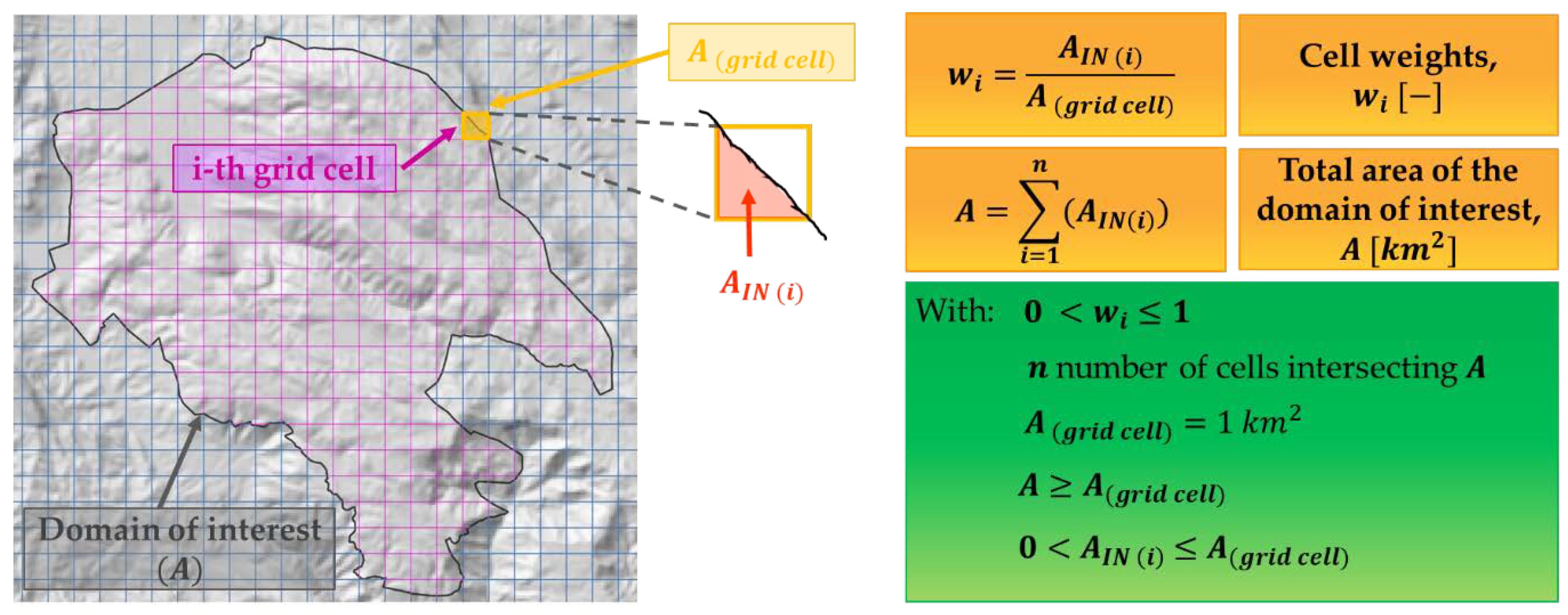
2.1. General Modelling Definitions

Traditionally, the definition of the water budget equation is based on the general principle of conservation of mass in a closed system [20]. In the specific case, for a selected continuous time interval ∆t, the total inflow into a given hydrological control unit (HCU) is equal to the outflow from the HCU, and can be expressed by the following relation:

$$\mathrm{IN} = \mathrm{OUT} + \mathsf{\Delta }\mathrm{S}$$

(1)

where:

• IN represents the inflow of water (i.e., precipitation) into the control hydrological unit in a given ∆t;
• OUT represents the outflow (i.e., evapotranspiration, runoff, infiltration) from the control hydrological unit in a given ∆t;
• ΔS represents the change in storage within the hydrological control unit in a given ∆t (positive if the outflow is less than the inflow, and negative otherwise).

Equation (1), depending on the study’s objectives and the scale of analysis (i.e., spatial and temporal scale), can be further discretized by reflecting the various components of the hydrological cycle. In fact, not all components are always necessary or of equal importance (i.e., some components may be of reduced or even negligible importance) in line with the purpose of the study and the spatial domain of interest.

Certainly, a further discriminating aspect for selecting Equation (1)’s components is determined by the availability and representativeness of the input data. Indeed, in situ monitoring networks are rarely designed to provide information homogeneously distributed over a territory, but often they reflect monitoring needs with purely site-specific logic. In actuality, the availability of sufficiently representative spatial and temporal input data represents a fundamental requirement in implementing a reliable water budget model.

Supplementary considerations on the competing factors in Equation (1) can be introduced considering the distinction between measured (i.e., precipitation, temperature, etc.) or analytically determined variables (i.e., evapotranspiration, solar radiation, etc.). According to WFD, these considerations could be accompanied by a further element of influence, namely the potential effects of the dynamism of the natural and anthropogenic processes. In such terms, the WFD identifies four main categories: (i) Climate change, which has direct consequences on precipitation and temperature [21]; (ii) water consumption, mainly influenced by the water demand variations in industrial, agricultural, and domestic sectors; (iii) the resilience of the infrastructure system, determined by the socio-economic, administrative factors or characteristics of a territory; and (iv) land-use changes, induced by the evolution of the anthropogenic footprint on a territory and its planning path.

As already mentioned, the definition of the modelling features (i.e., spatial scale, time scale, and simulation period) related to setting up a water budget framework are not determinable a priori. In fact, the choice of such characters depends on the study aim and on which responses are expected from the model itself [1].

For example, if the monitoring of drought phenomena is the target, it is preferable to implement a long-term (at least more than 20 years) water budget model with a wide spatial perspective (regional or inter-regional scale). As it is well known, climate processes are characterized by spatial migration during the temporal evolution, also propagating through the hydrological cycle with a signal periodicity peculiar to each component [22,23,24]. Hence, it is reasonable to consider that long series of precipitation and temperature values significantly characterize the interpretation of these phenomena [25].

On the other hand, in order to reproduce an adequate model capable of describing, for example, phenomena related to groundwater recharge (i.e., surface runoff, infiltration, etc.) over a specific hydro-geological unit, it is advisable to (i) refer to an adequate time discretization of the Δt factor in Equation (1) (i.e., daily scale) and (ii) consider the influence of the previous states to provide a continuous time evaluation of the different variables during the selected ∆t. Then, in order to capture the variation of the variables of interest, a sufficiently representative period (greater than 20 years) consisting in a sequence of a specific time interval (i.e., hydrological year, solar year, wet/dry season, multi-year period, etc.) must be implemented [1].

Finally, for proper interpretation of the water budget tool, the question that a user should ask about a given model is “How reliable is it?”. This question is not able to draw an immediate response; in fact, it is widespread as uncertainties and model reliability are affected by various factors. As mentioned, for a determined environmental system, the availability and the quality of the hydrological data, the knowledge of the geological and socio-economic boundary conditions, the schematization of the phenomena under study, etc., must be considered.

Furthermore, building a model without uncertainties is impossible by definition. The uncertainties related to a model within certain limits may possibly be reduced, but they need to be recognized, thereby the model’s outcomes remain adequately circumscribed within the assumptions made. In this respect, the performance of a water budget model should be defined a priori as a compromise between the responses to which one wishes to strive and the degree of reliability achievable.

Finally, it is worth noting that water budget models are generally developed to cover the following scopes of application:

• Producing different water resource management scenarios in order to assess (ex ante) their potential impact on water use, demand, and availability;
• Learning (ex-post) from the effects of mitigation actions implemented in the past to counteract possible drought and water-scarcity events.

In order to pursue these objectives, it is necessary to transfer advanced water management tools to decision-makers capable of supporting future planning that contemplates different possible environmental, climatic, and socio-economic scenarios [3,26,27].

To this end, it is possible to regard the water budget tool as part of a broader strategy, aiming at a paradigm shift in water resource management, turning towards a risk management strategy rather than facing emergencies.

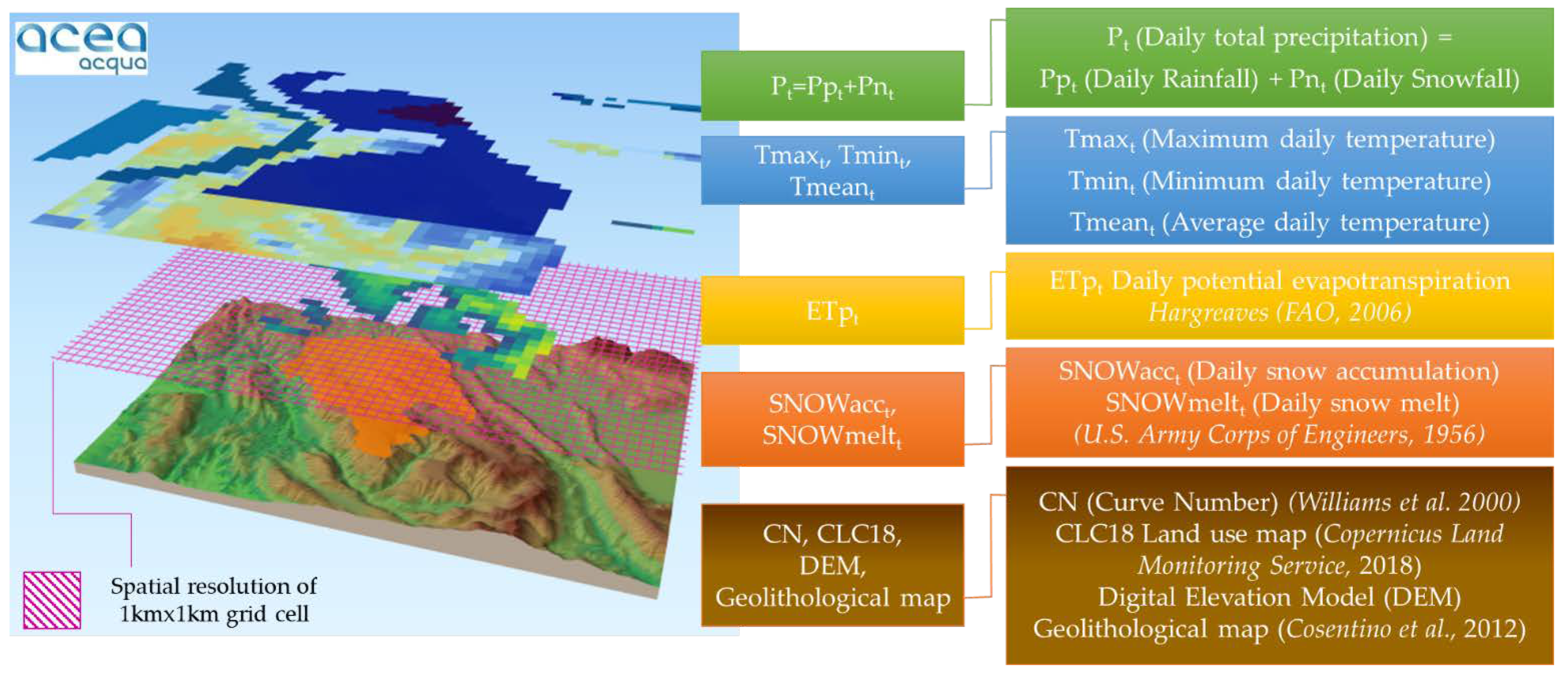
2.2. Framework of the Proposed Water Budget Model

In the following paragraphs, the technical criteria will be schematically described, in accordance with the WFD [28], implemented by Acea Ato2 for the assessment of the quantitative status of potential groundwater resources.

The proposed methodology follows a simple analytical approach, time-continuous and spatially distributed (grid-based), aimed at evaluating the groundwater resource status in the whole territory under management.

It is well known that reliable assessment of the water budget requires a modelling tool that allows continuous evaluation of the variables over time [29].

In light of the above, the first step in the development of a water budget model is the analytical definition of the hydrological cycle’s components to be taken into account. Traditionally, at the daily scale, the I.H.B. equation can be expressed as follows:

$${\mathrm{I}}_{\mathrm{t}}={\mathrm{P}}_{\mathrm{t}}-{\mathrm{ETp}}_{\mathrm{t}}-{\mathrm{R}}_{\mathrm{t}}$$

(2)

where ${\mathrm{I}}_{\mathrm{t}}$ is the daily infiltration [mm] at the current time step ($\mathrm{t}$), ${\mathrm{P}}_{\mathrm{t}}$ is the cumulative daily precipitation [mm], ${\mathrm{ETp}}_{\mathrm{t}}$ is the daily potential evapotranspiration [mm], and ${\mathrm{R}}_{\mathrm{t}}$ is the daily surface runoff [mm].

It goes without saying that, with reference to Equation (2), the accuracy of the proposed model is strictly dependent on the precipitation and temperature ($\mathrm{T}$) data available and on the knowledge of their spatial distribution over the domain of interest. In this respect, Acea Ato2 disposes of the hydrological time series processed by meteorological experts. Such time series are elaborated from measurements collected by ground-based instruments, subsequently integrated with radar observations, and finally spatialized over the entire managed territory using geo-statistical techniques. These time series exhibit a 30-year record length (since January 1990), a daily time step, and a 1 km spatial resolution (square regular cells).

Considering that mountain snowfields act as natural reservoirs for the water-supply system, storing precipitation, it is of utmost importance to first classify the precipitation occurring via rainfall (P_p) and snowfall (P_n), and then to incorporate the snowmelt and snow-accumulation processes in the I.H.B. model adopted. For this purpose, a criterion based on the average air temperature is implemented [30,31].

The ETp_t component is estimated indirectly from temperature, following here the Hargreaves empirical formulation [31,32].

The daily surface runoff component (R_t) is here evaluated by the Curve Number (CN) methodology modified by Williams [29]:

$${\mathrm{R}}_{\mathrm{t}}=\frac{{\left({\mathrm{P}}_{\mathrm{t}}-{\mathrm{Ia}}_{\mathrm{t}}\right)}^2}{\left({\mathrm{P}}_{\mathrm{t}}-{\mathrm{Ia}}_{\mathrm{t}}+{\mathrm{S}}_{\mathrm{t}}\right)}$$

(3)

where:

• ${\mathrm{Ia}}_{\mathrm{t}}$ is the initial losses [mm], i.e., the fraction of precipitation intercepted by the vegetation, filling in the surface cavities, etc.; the surface runoff occurs only when the daily precipitation is greater than the intercepted fraction. ${\mathrm{Ia}}_{\mathrm{t}}$ is usually assumed to be 0.2${\mathrm{S}}_{\mathrm{t}}$;
• ${\mathrm{S}}_{\mathrm{t}}$ is the retention coefficient [mm]. ${\mathrm{S}}_{\mathrm{t}}$ is the function of several parameters representing the soil type and its saturation, land use, and slope.

According to the original methodology [33], the coefficient $\mathrm{S}$ [mm] can be expressed as follows:

$$\mathrm{S}=25.4·\left(\frac{1000}{\mathrm{CN}}-10\right)$$

(4)

where the dimensionless parameter $\mathrm{CN}$ assumes values between 0 and 100, and under the same precipitation, as this value increases, the ability of soil to produce surface runoff increases.

Instead, the modified CN methodology proposed by Williams foresees the retention parameter adjustment according to Equation (5). In particular, ${\mathrm{S}}_{\mathrm{t}}$ assumes values within the range of 0 (saturated soil) to ${\mathrm{S}}_{\max }$ (dry soil), assigned as a function of the potential evapotranspiration ETp_t evaluated for the current time step, and of the rainfall (${\mathrm{P}}_{\mathrm{t}-1}$), surface runoff (${\mathrm{R}}_{\mathrm{t}-1}$) and retention coefficient (${\mathrm{S}}_{\mathrm{t}-1}$) related to the previous time step (i.e., previous day):

$${\mathrm{S}}_{\mathrm{t}}={\mathrm{S}}_{\mathrm{t}-1}+{\mathrm{ETp}}_{\mathrm{t}}·\exp \left(\frac{-{\mathrm{BS}}_{\mathrm{t}-1}}{{\mathrm{S}}_{\max }}\right)-{\mathrm{P}}_{\mathrm{t}-1}+{\mathrm{R}}_{\mathrm{t}-1}$$

(5)

$${\mathrm{S}}_{\max }=25.4·\left(\frac{1000}{\mathrm{CN}\left(\mathrm{I}\right)}-10\right)$$

(6)

$${\mathrm{S}}_{\mathrm{t}=0}=25.4·\left(\frac{1000}{\mathrm{CN}\left(\mathrm{II}\right)}-10\right)$$

(7)

where:

$\mathrm{B}$ is the depletion coefficient [dimensionless], theoretically varying from 0 to 2 (here assumed to be 1).

$\mathrm{CN}\left(\mathrm{II}\right)$ is the curve number evaluated according to the degree of saturation of the soil under normal conditions. It is obtained through specific tables provided by the Soil Conservation Service [33], while $\mathrm{CN}\left(\mathrm{I}\right)$ and $\mathrm{CN}\left(\mathrm{III}\right)$ are calculated in dry and saturated soil conditions, respectively.

Since $\mathrm{CN}\left(\mathrm{II}\right)$ values depend on both geological and hydrological soil characteristics (i.e., permeability, soil texture, land use, etc.), here we referred to the latest version of CORINE Land Cover (CLC18) [34] and the regional geolithological map [35] to acquire information on the study area’s land use and to define the relative soil hydrological group, respectively. Subsequently, as suggested by Williams [36], an adjustment to the $\mathrm{CN}\left(\mathrm{II}\right)$ value is introduced with respect to the terrain’s slope: ($\mathrm{CN}\left(\mathrm{II}\right)\mathrm{s}$). The modified value of ($\mathrm{CN}\left(\mathrm{II}\right)\mathrm{s}$) is calculated once a digital elevation model (DEM) is available for the domain of interest.

Referring to the above-mentioned definitions, in Figure 1, the main inputs of the water budget model implemented in the study are depicted.

In favor of simplicity, Figure 2 shows the spatial schematization applied for the evaluation of each model’s component within the i-th grid cell on which any selected domain of interest (A) is discretized. It is worth noting the proposed water budget framework is performed on each cell independently of each other, without considering physical connections between them.

In coherence with the spatial resolution of the hydrological components, geolithological, altimetric, and land use data are spatially discretized within a 1 km grid cell.

It should be pointed out that solving the I.H.B. equation at the daily scale and for the i-th grid cell may generate an analytical drawback in the estimation of the ${\mathrm{I}}_{{\mathrm{t}}_{\left(\mathrm{i}\right)}}$ component (potential daily infiltration computed within the i-th grid cell). In short, during the days with low or absent precipitation, the ${\mathrm{I}}_{{\mathrm{t}}_{\left(\mathrm{i}\right)}}$ component would be less than zero (a physics non sequitur) considering that ${\mathrm{ETp}}_{{\mathrm{t}}_{\left(\mathrm{i}\right)}}$ is always positive. Therefore, at the current state of modelling, the value of infiltration evaluated at the daily scale (or higher) can be considered an objective index for qualitative assessment rather than an actual cumulative volumetric measure. Clearly, in order to ensure model consistency with the physical boundary conditions, as introduced in Equation (8), no percolation in the soil is assumed in the case where I_t(i) manifests a negative value.

$$\{\begin{array}{c}\left({ \mathrm{P}}_{\mathrm{t}}{}_{\left(\mathrm{i}\right)}-{\mathrm{ETp}}_{{\mathrm{t}}_{\left(\mathrm{i}\right)}}-{\mathrm{R}}_{{\mathrm{t}}_{\left(\mathrm{i}\right)}}\ge 0\right)\to { \mathrm{I}}_{{\mathrm{t}}_{\left(\mathrm{i}\right)}}={ \mathrm{P}}_{\mathrm{t}}{}_{\left(\mathrm{i}\right)}-{\mathrm{ETp}}_{{\mathrm{t}}_{\left(\mathrm{i}\right)}}-{\mathrm{R}}_{{\mathrm{t}}_{\left(\mathrm{i}\right)}}\\ \left({ \mathrm{P}}_{\mathrm{t}}{}_{\left(\mathrm{i}\right)}-{\mathrm{ETp}}_{{\mathrm{t}}_{\left(\mathrm{i}\right)}}-{\mathrm{R}}_{{\mathrm{t}}_{\left(\mathrm{i}\right)}}<0\right)\to { \mathrm{I}}_{{\mathrm{t}}_{\left(\mathrm{i}\right)}}=0\end{array}$$

(8)

According to the notation introduced in Figure 2, the daily potential infiltration over a selected domain of interest (I_t(A)) can be estimated by considering ${\mathrm{I}}_{{\mathrm{t}}_{\left(i\right)}}$ values computed for each i-th cell and then performing the following expression within the selected area (A):

$${\mathrm{I}}_{\mathrm{t}\left(\mathrm{A}\right)}=\frac{{\sum }_{\mathrm{i}=1}^{\mathrm{n}}({\mathrm{I}}_{{\mathrm{t}}_{\left(\mathrm{i}\right)}}·{\mathrm{A}}_{\mathrm{IN}\left(\mathrm{i}\right)})}{{\sum }_{\mathrm{i}=1}^{\mathrm{n}}{\mathrm{w}}_{\mathrm{i}}}$$

(9)

Subsequently, as introduced in Equation (10), it is reasonable to calculate the potential infiltration for different time scales I_kt(A) (i.e., decadal, monthly, seasonal, etc.) by aggregating the I_t(A) values over time.

$${\mathrm{I}}_{\mathrm{kt}\left(\mathrm{A}\right)}={\displaystyle \sum }_{\mathrm{j}=1}^{{\mathrm{k}}_{\mathrm{t}}}{\mathrm{I}}_{\mathrm{t}\left(\mathrm{A}\right)}$$

(10)

with:

$${\mathrm{k}}_{\mathrm{t}}= \mathrm{k}·\mathrm{t} \{\begin{array}{c} \mathrm{k}>1\\ \mathrm{k}\in \mathbb{N}\end{array}$$

(11)

As mentioned, in adherence to the water management requirements, one of the primary purposes of the study is to provide straightforward tools for the evaluation of the aquifers’ potential recharge status with respect to the historical reference conditions. With this perspective, for further interpretation of Equation (2), here we propose the introduction of a functional index, defined as the normalized annual infiltration rate (I_N).

The normalized annual infiltration index over a domain of interest and for a selected hydrological year (in this study, defined between 1 September and 31 August), ${\mathrm{I}}_{\mathrm{N}\left(\mathrm{A}\right)}^{*}$, is assessed as the ratio between the infiltration values evaluated for a selected hydrological year ${\mathrm{I}}_{\left(\mathrm{A}\right)}^{*}$ and the long-term infiltration average $\overline{{\mathrm{I}}_{\left(\mathrm{A}\right)}}$ evaluated for the entire time series record length (i.e., 30 years). As a consequence, ${\mathrm{I}}_{\mathrm{N}\left(\mathrm{A}\right)}^{*}$ is defined by the following simple expression:

$${\mathrm{I}}_{\mathrm{N}\left(\mathrm{A}\right)}^{*}=\frac{{\mathrm{I}}_{\left(\mathrm{A}\right)}^{*}}{\overline{{\mathrm{I}}_{\left(\mathrm{A}\right)}}}$$

(12)

By solving Equation (12), an immediate measure of the aquifers’ potential recharge status over a selected domain of interest is provided.

Consequently, comparing the two terms in Equation (12) allows one to propose the ${\mathrm{I}}_{\mathrm{N}\left(\mathrm{A}\right)}^{*}$ ranking with respect to the long-term average condition, as follows:

$${\mathrm{I}}_{\mathrm{N}\left(\mathrm{A}\right)}^{*}=\{\begin{array}{c}\ge 0 Ʌ<1, {\mathrm{I}}_{\left(\mathrm{A}\right)}^{*}<\overline{{\mathrm{I}}_{\left(\mathrm{A}\right)}} \mathrm{below} \mathrm{long}-\mathrm{term} \mathrm{average} \mathrm{condition}\\ =1, { \mathrm{I}}_{\left(\mathrm{A}\right)}^{*}=\overline{{\mathrm{I}}_{\left(\mathrm{A}\right)}} \mathrm{equal} \mathrm{to} \mathrm{long}-\mathrm{term} \mathrm{average} \mathrm{condition}\\ >1, { \mathrm{I}}_{\left(\mathrm{A}\right)}^{*}>\overline{{\mathrm{I}}_{\left(\mathrm{A}\right)}} \mathrm{above} \mathrm{long}-\mathrm{term} \mathrm{average} \mathrm{condition}\end{array}$$

(13)

If, on the one hand, the direct application of the water budget equation plays a key role for the aquifers’ potential recharge status estimation, on the other hand, it is deemed appropriate to introduce further control quantities.

In particular, it is certainly possible to include continuous monitoring of the rainfall trends, here performed through the spatial analysis of the widespread Standardized Precipitation Index (SPI) over the domain of interest [19]. The SPI is a flexible index widely used to identify drought phenomena in terms of the precipitation deficit (or surplus) compared to the long-term climatological average [37].

In this study, monitoring rainfall trends through different aggregation time scales of cumulated precipitation (i.e., SPI scales) has been deemed representative [38]. In particular, referring to the monthly sequence identified by the hydrological year, the selected SPI scales are:

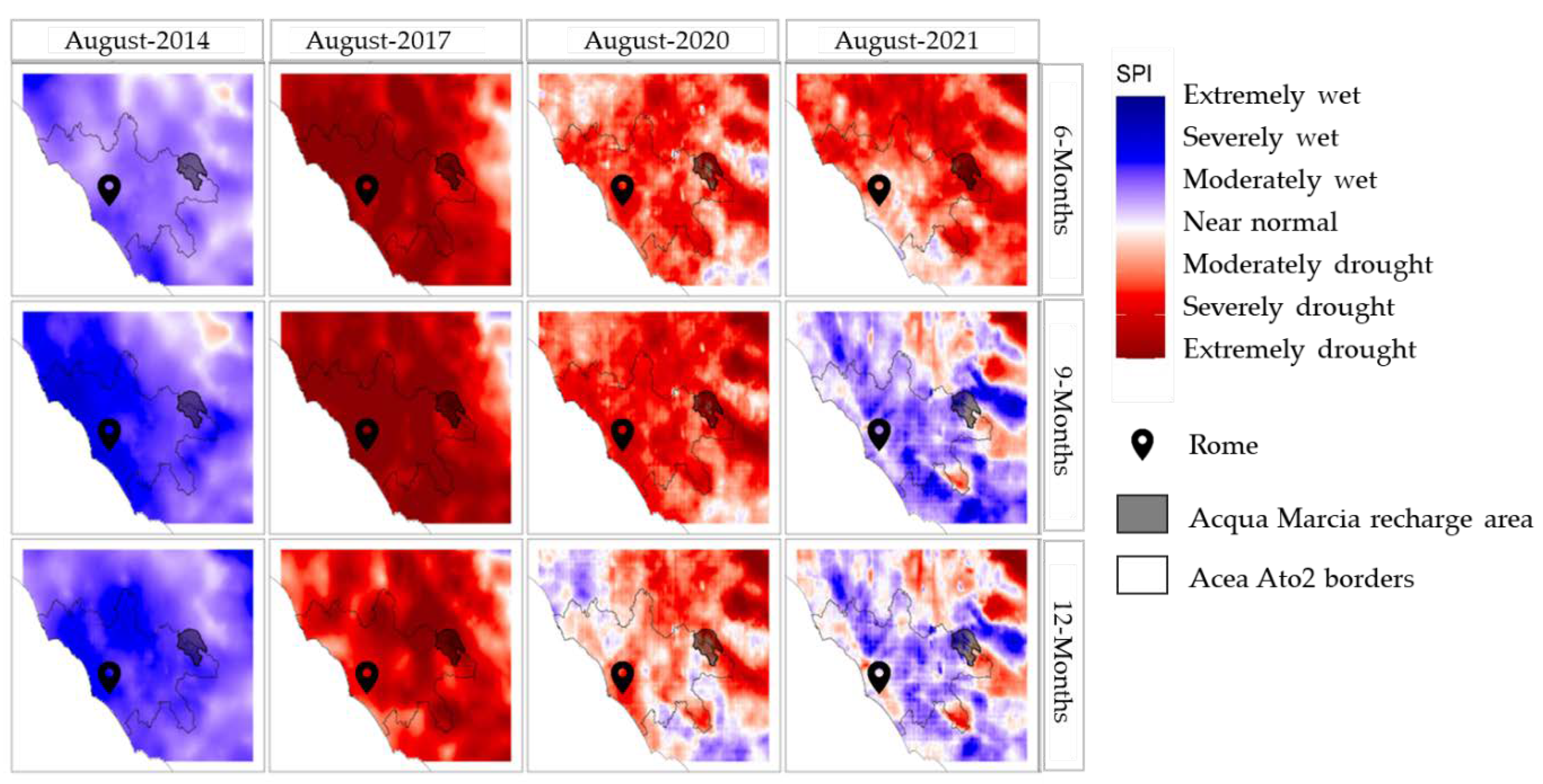
• 6 months, representing the precipitation between March and August (i.e., the cumulative precipitation of the spring–summer seasons);
• 9 months, representing the precipitation between December and August (i.e., the cumulative precipitation of the winter–spring–summer seasons);
• 12 months, corresponding to the cumulative precipitation during the entire hydrological year (September–August), therefore also finally including the autumn season’s precipitation.

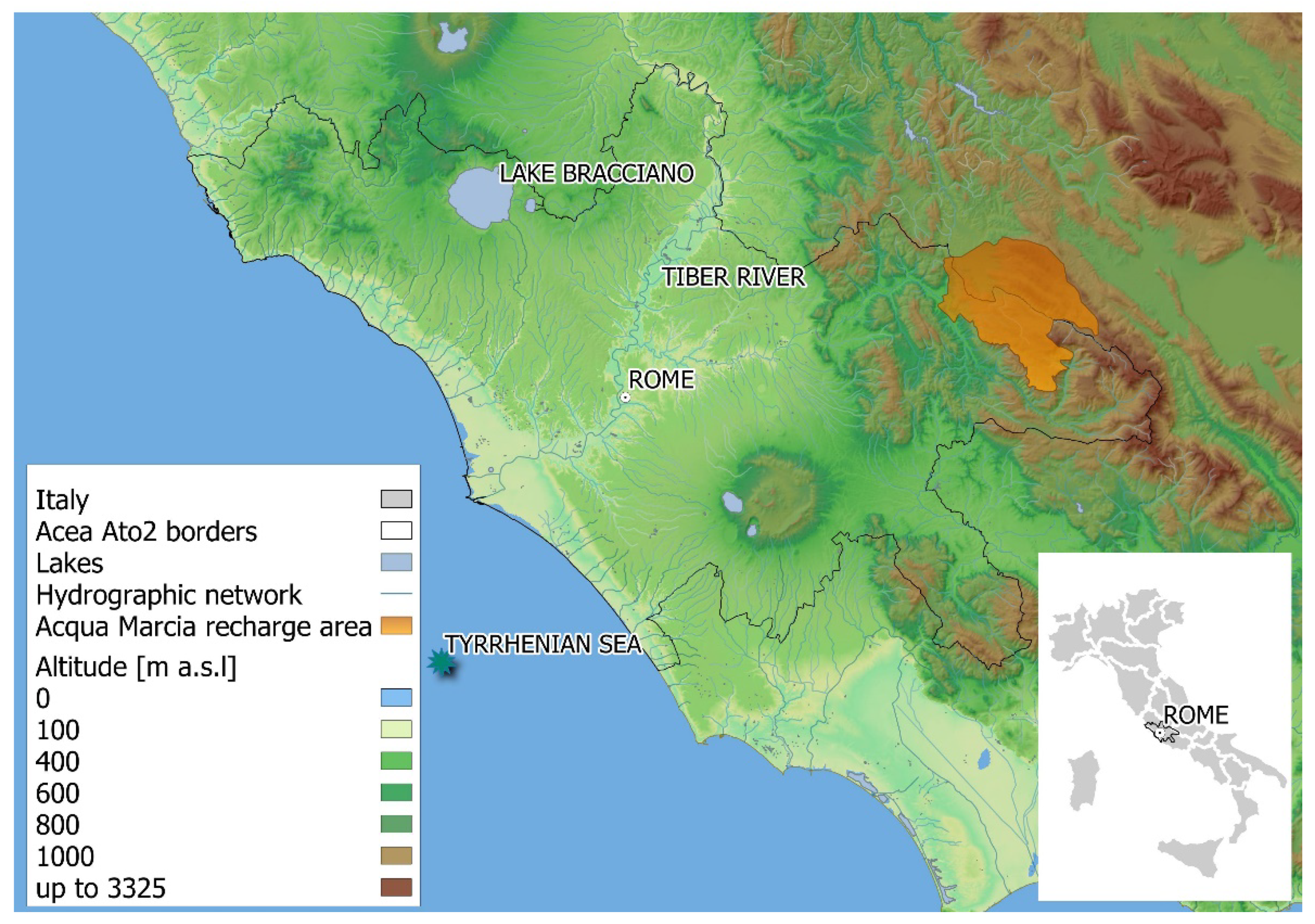
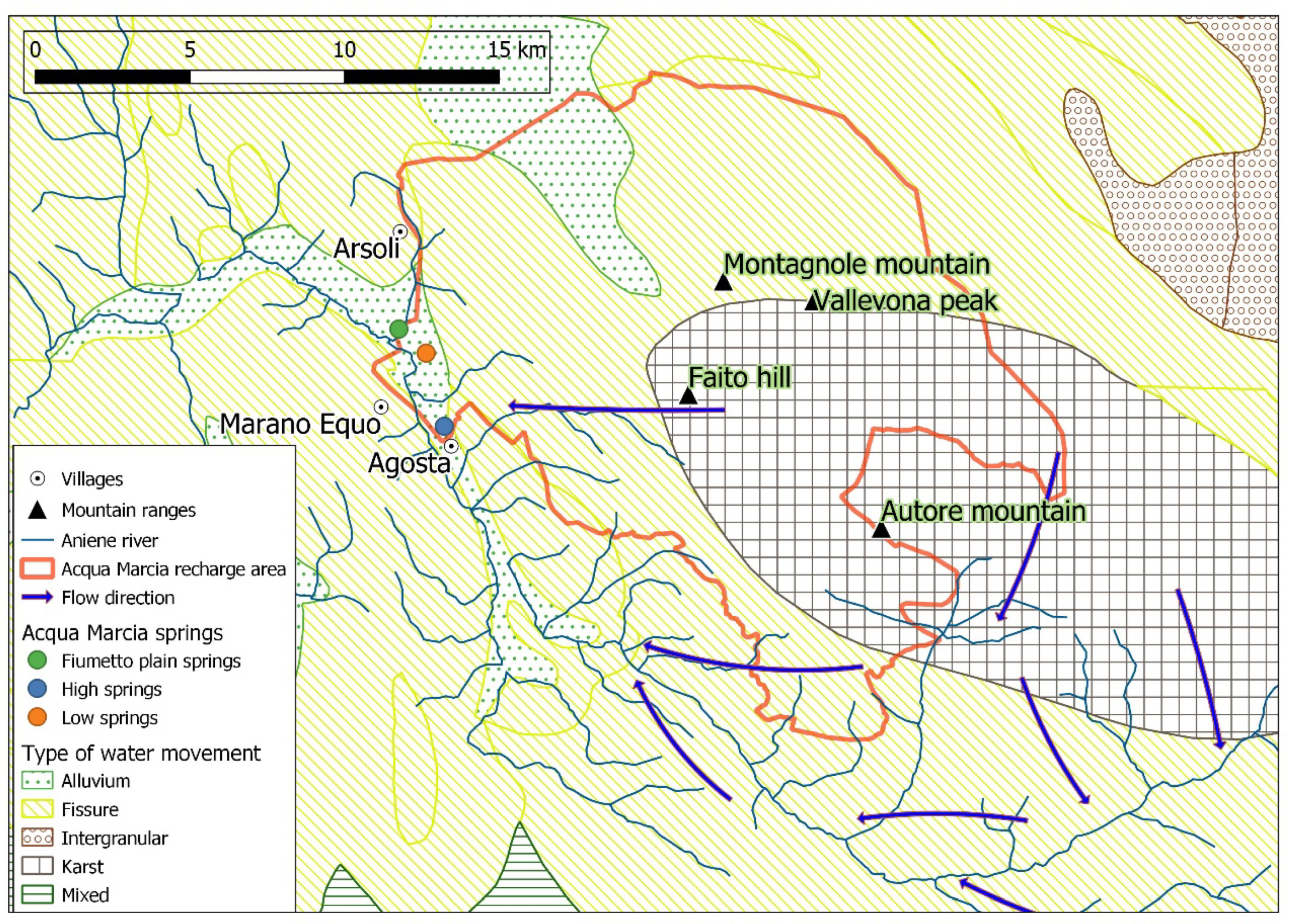
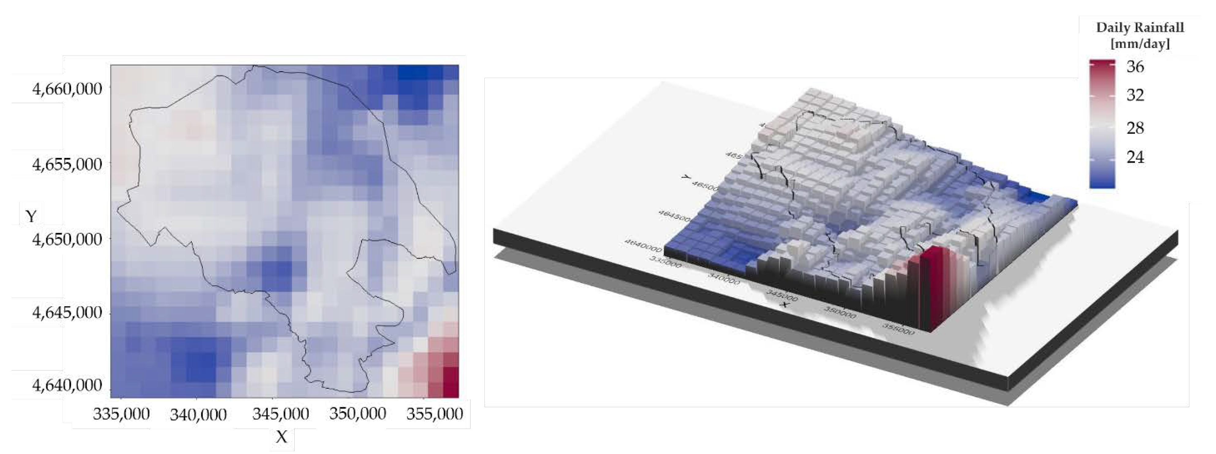
2.3. Study Area

The study area is represented by the management area of Acea Ato2, located in central Italy. The total area is about 5.400 km² in which more than 15.000 km of the water distribution network is deployed. The area is characterized by hilly zones and is bordered by the Tyrrhenian Sea and the Apennine ridge, to the West and East, respectively.

The central Italy Apennine area is of particular interest, in the panorama of karst carbonate aquifers in the Mediterranean context, for the distribution of water resources, as over 4 million users are fed by the springs located there (Figure 3).

The aquifers of central Italy generally consist of very diffuse karst hydrostructures [39]. Consequently, the different springs’ hydrograph phases are more responsive to the long-term driving forces compared to the effects provided by single and recent events [38].

In the current study, among the managed aquifers of Acea Ato2, the Acqua Marcia springs that supply a historical aqueduct of Rome have been selected as the case study.

The Acqua Marcia springs are located 50 km from Rome, fed by Apennine hydrostructures situated in the Latium-Abruzzi platform ridge over the protected area of the Simbruini Mountains (from the Latin sub imbribus, under the rains) and bordered by the middle valley of the Aniene river (Figure 4).

The Acqua Marcia hydrosystem is composed of different groups of springs, classifiable in reference to the altitude of the water emergences:

(a)

High springs, located at a water table level between 329 m and 326 m asl at the base of the hilly relief where the village of Agosta is settled;

(b)

Low springs, with a water table level between 324 m and 321 m asl, near the Marano Equo village;

(c)

Fiumetto plain springs, located between 322 and 321 m asl, within the Arsoli valley.

These springs are fed by meteoric inflows that produce net infiltration values of about 890 mm/year [38,40], in a recharge area of about 250 km².

The spring discharge produced by the Acqua Marcia hydrosystem, with an annual average value of about 5 m³/s, feeds an aqueduct system composed of two conduits that run parallel to the Aniene river valley. The two conduits are named I and II Marcio pipelines, and the latter was built around the end of the 19th century while the former is relatively more recent and was constructed between 1924 and 1928.

The Acqua Marcia aqueduct system conveys approximately 25% of the water resource demand of the city of Rome, representing the second-largest aqueduct system (after the Peschiera-Capore aqueduct system) of the water distribution network managed by Acea Ato2.

3. Application of the Methodology to the Case Study Acqua Marcia Springs

In the current section, the main results of the proposed methodology are presented, carried out for the entire reference period (January 1990–August 2021) and applied to the case study of the Acqua Marcia springs.

Practically, the water budget equation (i.e., Equation (2) and those following) can be evaluated once (i) the polygonal shapefiles (aquifer recharge areas, catchment areas, administrative units, etc.), (ii) rainfall and temperature time series (Network Common Data Form- NetCDF format) (Figure 5), and (iii) raster data (grid format) with information related to hydrogeological groups, CN(II) values, and ground elevation (i.e., DEM) are available.

In order to compare the potential recharge status of the Acqua Marcia springs with respect to the long-term infiltration average, Figure 6 reports the cumulative frequency distribution of the normalized annual infiltration rate (I_N(A)).

By analyzing the frequency distribution of I_N(A) values reported in Figure 6, the following considerations can be introduced:

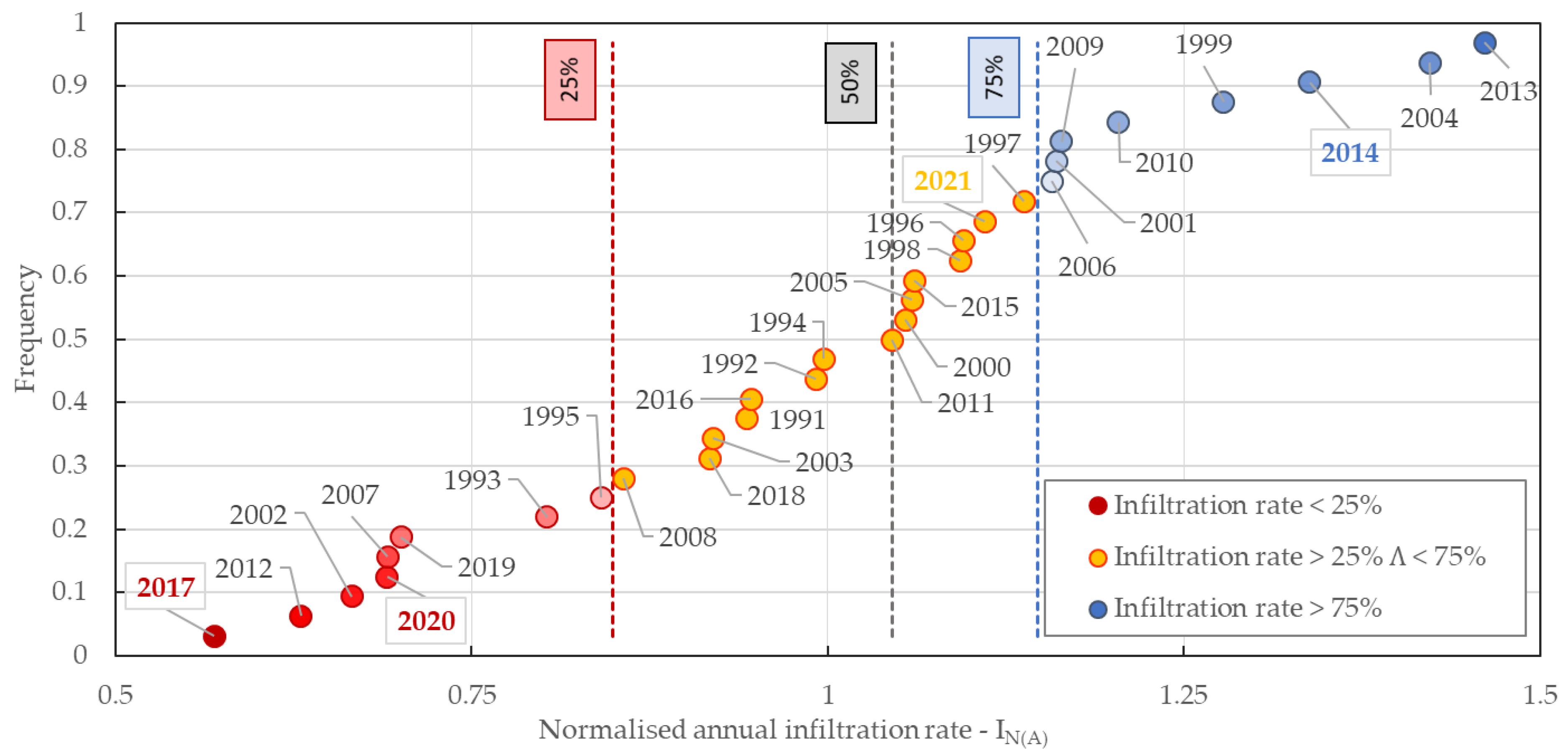
• Modest negative asymmetry in the distribution of the frequency values can be appreciated, and the mean value tends to be slightly lower than the 50th percentile;
• An appreciable range (slightly less than ±0.5) around the normalized mean value affected the frequency distribution. This implies that the infiltration rates representative of extremely dry (or wet) hydrological years can differ by up to approximately 50% from the long-term average condition;
• I_N(A) values included in the lower tail of the frequency distribution are representative of the most-severe drought events of the last 30 years, which occurred in the second decade of the 2000s;
• I_N(A) values included in the upper tail of the frequency distribution mainly occurred during the first decade of the 2000s;
• I_N(A) values calculated for the last 20 years show a wide dispersion, including both the upper and the lower values of the whole sample.

It is well known that a proper climatic phenomena interpretation over an area is conditioned by the adoption of an adequate scale of analysis in both spatial and temporal terms [23,41].

In this regard, in order to reproduce a wide spatial perspective, Figure 7 depicts the SPI values calculated for each cell within the entire managed area of Acea Ato2 and the surrounding territory.

As previously introduced, SPI values shown in Figure 7 refer to three selected time scales (i.e., 6, 9, 12 months) and are evaluated in correspondence with four different hydrological years introduced as comparison conditions.

In particular, the hydrological years of interest have been selected on the basis of the I_N(A) percentile classes (as defined in Figure 6). The following hydrological years were selected:

• 2014, I_N(A) > 75th percentile;
• 2017 and 2020, I_N(A) < 25th percentile;
• 2021, 50th percentile < I_N(A) < 75th percentile.

Figure 7 suggests both extremely wet periods (hydrological year 2014) and extremely dry periods (hydrological year 2017) tend to homogeneously involve wide geographical areas and are prolonged over several hydrological years.

Moreover, referring to the 12-month SPI scale, what emerges is that a lack of, or reduced, contribution of the late autumn and winter precipitation (both liquid and snowy) can seriously affect the groundwater recharge status, as occurred during the hydrological year 2020. Alternatively, although a reduced amount of spring rainfall occurs, an abundant inflow rate during the autumn and winter seasons (such as during the hydrological year 2021) succeed in mitigating possible water-scarcity events.

4. Discussion and Conclusions

In the present study, Acea Ato2, a water utility operating in central Italy (Latium region), proposes a simple analytical water budget model for assessing the potential recharge of the managed aquifers. In this context, the evaluation of the groundwater resources’ status embraces the wider environmental and socio-economic objectives outlined by the Water Framework Directive issued by the European Commission.

The proposed methodology is coded in R (an open-source environment), and requires a time series of precipitation and temperature spatially distributed over the domain of interest as main inputs. In this respect, Acea Ato2 disposes of daily time series with a 30-year record length, spatially distributed within the entire managed area and the surrounding territory with a 1 km resolution (square regular cells).

In addition to the hydrological time series, in this study, we use open-input geographical data (raster and shapefile) that require limited pre-processing operations. In this regard, it can be pointed out that the use of open data and open-source software environments allows any other users (i.e., water managers) to facilitate the reproducibility of the methodology [15,16].

Furthermore, a practical advantage of the adopted water budget framework is that it requires a reduced number of inputs, in accordance with the parsimony philosophy [11]. Moreover, a simple and parsimonious methodology is functional in terms of (i) any users’ level of expertise, (ii) whether the existing data in a territory do not suffice to develop a detailed model, and (iii) whether the study’s aim involves a wide range of spatial and temporal scales [9].

On the other hand, it is worth noting that the level of detail and uncertainty incorporated into any water budget model depends on the study’s objectives and the data availability. In fact, the proposed approach may lead to high uncertainties because of errors accumulated in all terms of the water budget equation [42].

Likely, the potential evapotranspiration is the term that includes the greatest uncertainty in its evaluation. In fact, considering that ETp’s in situ measurements often are not sufficiently widespread, usually the ETp is indirectly calculated through other variables. In this work, to evaluate the ETp, the empirical expression of Hargreaves is applied, although its representativeness for the climatic zone under study needs to be further investigated. The choice of the Hargreaves formulation is motivated by its nature of being easy to implement for the proposed framework and parsimonious in terms of required inputs (i.e., daily series of maximum and minimum temperature are requested) [25]. Furthermore, at the current modelling status, ETp is used instead of the actual evapotranspiration. For further model improvement, the crop coefficient should be introduced to consider the vegetative influence on evapotranspiration.

Obviously, the uncertainty inherent in the water budget’s equation terms affects the potential infiltration assessment. In particular, considering that ETp always assumes positive values, solving the water budget equation during days with low or absent precipitation could lead to negative values of the I_t component. This finds rationale since part of the rainfall that reaches the soil is temporarily stored (bucket effect) in the zone identified by the vegetation root system (i.e., root zone) [20,43]. In the root zone, different processes take place: Water absorption due to rain and snowmelt, depletion due to evapotranspiration processes, and possible runoff when the soil is saturated. Although this constitutes an issue to be addressed, in adherence to the goals established in this study, from a water manager’s point of view, the current I_t evaluation already represents a convenient compromise to quantify the potential groundwater recharge status.

Although it should be considered that the simplified formulation of the water budget framework does not allow for capturing the whole complexity of hydrological processes (i.e., climatic, hydrological and hydrogeological), here they are evaluated on the basis of a spatially distributed and time-continuous framework.

In this regard, it is worth noting that the proposed water budget framework is performed cell by cell, without considering physical connections between them. This leads to a discontinuous assessment of the inflow and the outflow volumes. These divergences become more significant when hydrodynamics processes over an area are governed by surface water flows [4]. Indeed, the current model transposes the assumptions that the major rate of the potential infiltration within the domain of interest is due to groundwater system exchanges [40].

Simultaneously, among the aspects related to time-continuous modelling, it is notable to mention the impact of land-use change over time, as it directly affects the surface water runoff and absorption (and therefore infiltration) capacity of the soil. In fact, at the current state, the proposed framework does not include an input able to reproduce land-use change over the time. In fact, for the sake of simplicity, here we refer to the latest version of CLC18 over the entire selected period of observation. Consequently, in a forthcoming release of the study, it would be advisable to model and evaluate the effects induced by the evolution of the anthropogenic footprint on the study area. However, it should also be considered that the managed aquifers of Acea Ato 2 are mainly located in areas prone to severe land-use restrictions. Hence, as the first hypothesis, it is reasonable to consider the land-use change over the observation period and its effects on the water budget evaluation almost negligible.

In light of the present investigation carried out, it was found that the proposed water budget model could successfully cover several water managers targets. At the same time, in order to improve the actual model, we need to deal with the above-mentioned gaps, data gaps, and issues, and these should be addressed on an ongoing basis. In fact, within the limits of the simplifications introduced, the model can provide an initial understanding of the hydrological processes and support stakeholders in water resource management.

In this regard, the current study reports the preliminary results offered by the adopted water budget model, relative to the case study of the Acqua Marcia springs. Apart from computing the water budget equation, the aim of the study is to provide interpretative tools to determine the potential groundwater recharge status. Hence, in order to conduct continuous monitoring of the rainfall trends and the potential recharge status of the aquifers with respect to the historical reference conditions, here we have implemented, respectively, spatial analysis of the SPI and the normalized annual infiltration rate (I_N).

Besides the analytical and interpretative aspect of the phenomena, what emerges from the application of the proposed methodology is that for a rational and integrated understanding of water systems:

• It is essential to implement studies with a long-term duration and a wide spatial perspective. In fact, in order to perform appropriate monitoring of water resources and in particular to intercept potential drought events in advance, it is necessary, on one hand, according to the traditional methodological approach, to determine the frequency, duration, and spatial domain over which the phenomena extend [44]; on the other hand, it must be considered that the climate processes tend to propagate through the hydrological cycle [22,24], gradually influencing the different components (i.e., precipitation, soil moisture, infiltration, groundwater recharge, and spring flows). In this regard, several authors ([23,45] among others) argue that the propagation of the drought signal reaches the groundwater components often slowly or not at all, but when this occurs, drought produces severe and long-lasting consequences.
• It is desirable that water managers, practitioners, and public authorities refer to the same robust and well-grounded methodologies, because relying on the same methodology allows readily monitoring and reliably quantifying the water resources’ status in an area.

Although the proposed methodology is to be considered in a preliminary stage, in conclusion, we maintain that from a water manager’s perspective, it represents a reliable approach to rationalize medium- and long-term interventions aimed at reducing the vulnerability of the water supply system and to support the sustainability of withdrawals.

References

1. EU Commission. Guidance Document on the Application of Water Balances for Supporting the Implementation of the WFD. 2015. Available online: http://www.emwis.org/initiatives/pawa/background/guidance-document-application-water-balances-supporting-implementation-wfd (accessed on 3 October 2019).
2. Borzì, I.; Bonaccorso, B.; Aronica, G.T. The Role of DEM Resolution and Evapotranspiration Assessment in Modeling Groundwater Resources Estimation: A Case Study in Sicily. Water 2020, 12, 2980. [Google Scholar] [CrossRef]
3. Viaroli, S.; Mastrorillo, L.; Lotti, F.; Paolucci, V.; Mazza, R. The groundwater budget: A tool for preliminary estimation of the hydraulic connection between neighboring aquifers. J. Hydrol. 2018, 556, 72–86. [Google Scholar] [CrossRef]
4. Preziosi, E.; Romano, E. Dall’analisi idrostrutturale allo studio modellistico di acquiferi regionali. Ital. J. Eng. Geol. Environ. 2009, 1, 183–198. [Google Scholar]
5. Mineo, C.; Ridolfi, E.; Napolitano, F.; Russo, F. The areal reduction factor: A new analytical expression for the Lazio Region in central Italy. J. Hydrol. 2018, 560, 471–479. [Google Scholar] [CrossRef]
6. Beven, K. Changing ideas in hydrology—The case of physically-based models. J. Hydrol. 1989, 105, 157–172. [Google Scholar] [CrossRef]
7. Konikow, L.F.; Bredehoeft, J.D. Ground-water models cannot be validated. Adv. Water Resour. 1992, 15, 75–83. [Google Scholar] [CrossRef]
8. Gondwe, B.R.; Merediz-Alonso, G.; Bauer-Gottwein, P. The influence of conceptual model uncertainty on management decisions for a groundwater-dependent ecosystem in karst. J. Hydrol. 2011, 400, 24–40. [Google Scholar] [CrossRef]
9. Borzì, I.; Bonaccorso, B. Quantifying Groundwater Resources for Municipal Water Use in a Data-Scarce Region. Hydrology 2021, 8, 184. [Google Scholar] [CrossRef]
10. Braca, G.; Bussettini, M.; Ducci, D.; Lastoria, B.; Mariani, S. Evaluation of national and regional groundwater resources under climate change scenarios using a GIS-based water budget procedure. Rend. Lincei. Sci. Fis. E Nat. 2019, 30, 109–123. [Google Scholar] [CrossRef]
11. Koutsoyiannis, D. Seeking Parsimony in Hydrology and Water Resources Technology. In Proceedings of the European Geosciences Union General Assembly 2009, Vienna, Austria, 19–24 April 2009; Geophysical Research Abstracts: Vienna, Austria, 2009; Volume 11, p. 11469. [Google Scholar]
12. R Core Team. R: A Language and Environment for Statistical Computing; R Foundation for Statistical Computing: Vienna, Austria, 2020; Available online: https://www.R-project.org/ (accessed on 4 February 2020).
13. Slater, L.J.; Thirel, G.; Harrigan, S.; Delaigue, O.; Hurley, A.; Khouakhi, A.; Prosdocimi, I.; Vitolo, C.; Smith, K. Using R in hydrology: A review of recent developments and future directions. Hydrol. Earth Syst. Sci. 2019, 23, 2939–2963. [Google Scholar] [CrossRef] [Green Version]
14. Van Rossum, G.; Drake, F.L. Python 3 Reference Manual; CreateSpace: Scotts Valley, CA, USA, 2009. [Google Scholar]
15. Vorobevskii, I.; Kronenberg, R.; Bernhofer, C. Global BROOK90 R package: An automatic framework to simulate the water balance at any location. Water 2020, 12, 2037. [Google Scholar] [CrossRef]
16. Li, X.; Vernon, C.R.; Hejazi, M.I.; Link, R.P.; Feng, L.; Liu, Y.; Rauchenstein, L.T. Xanthos–a global hydrologic model. J. Open Res. Softw. 2017, 5, 1–7. [Google Scholar] [CrossRef] [Green Version]
17. Rossi, M.; Donnini, M. Estimation of regional scale effective infiltration using an open source hydrogeological balance model and free/open data. Environ. Model. Softw. 2018, 104, 153–170. [Google Scholar] [CrossRef]
18. Zini, L.; Calligaris, C.; Treu, F.; Zavagno, E.; Iervolino, D.; Lippi, F. Groundwater sustainability in the Friuli Plain. Acqua Mundi 2013, 4, 41–54. [Google Scholar]
19. McKee, T.B.; Doesken, N.J.; Kleist, J. The relationship of drought frequency and duration to time scales. In Proceedings of the 8th Conference on Applied Climatology, Anaheim, CA, USA, 17–22 January 1993; Volume 17, pp. 179–183. [Google Scholar]
20. Chow, V.T. Handbook of Applied Hydrology; McGraw-Hill: New York, NY, USA, 1965. [Google Scholar]
21. Panagoulia, D.; Dimou, G. Sensitivities of groundwater-streamflow interaction to global climate change. Hydrol. Sci. J. 1996, 41, 781–796. [Google Scholar] [CrossRef] [Green Version]
22. Mineo, C.; Passaretti, S.; Varriale, A. Drought risk analysis and spring discharge forecasting: A coupled method for an optimal fresh water management, ICNAAM 2020. In Proceedings of the 18th International Conference of Numerical Analysis and Applied Mathematics, Rhodes, Greece, 17–23 September 2020. [Google Scholar]
23. Van Loon, A.F. Hydrological drought explained. Wiley Interdisciplinary Reviews. Water 2015, 2, 359–392. [Google Scholar]
24. Changnon, S.A., Jr. Detecting Drought Conditions in Illinois; Circular 169; Illinois State Water Survey: Champaign, IL, USA, 1987. [Google Scholar]
25. Mariani, S.; Braca, G.; Romano, E.; Lastoria, B.; Bussettini, M. Linee Guida Sugli Indicatori di Siccità e Scarsità Idrica da Utilizzare Nelle Attività Degli Osservatori Permanenti per gli Utilizzi idrici—Stato Attuale e Prospettive Future; Technical Report. 2018. Available online: http://www.isprambiente.gov.it/files2018/notizie/LineeGuidaPubblicazioneFinaleL6WP1_concopertina.pdf (accessed on 18 April 2019).
26. Peres, D.J.; Modica, R.; Cancelliere, A. Assessing future impacts of climate change on water supply system performance: Application to the Pozzillo Reservoir in Sicily, Italy. Water 2019, 11, 2531. [Google Scholar] [CrossRef] [Green Version]
27. Sappa, G.; De Filippi, F.M.; Iacurto, S.; Grelle, G. Evaluation of minimum karst spring discharge using a simple rainfall-input model: The case study of Capodacqua di Spigno Spring (Central Italy). Water 2019, 11, 807. [Google Scholar] [CrossRef] [Green Version]
28. Mineo, C.; Passaretti, S.; Varriale, A.; Cosentino, C. A grid based model for a continuous time evaluation of water balance: A water manager’s perspective on the estimation of the status of water resources, IDRA2020. In Proceedings of the XXXVII Convegno Nazionale di Idraulica e Costruzioni Idrauliche, Reggio Calabria, Italy, 14–16 June 2021. [Google Scholar]
29. Williams, J.R.; Arnold, J.G.; Srinivasan, R. The APEX Model; BRC Report No. 00–06; Blackland Research and Extension Center, Texas Agricultural Experiment Station; Texas A & M University System: Temple, TX, USA, 2000. [Google Scholar]
30. U.S. Army Corps of Engineers. Snow Hydrology; North Pacific Division: Portland, OR, USA, 1956.
31. Percopo, C.; Brandolin, D.; Canepa, M.; Capodaglio, P.; Cipriano, G.; Gafà, R.; Iervolino, D.; Marcaccio, M.; Mazzola, M.; Mottola, A.; et al. Criteri tecnici per l’analisi dello stato quantitativo e il monitoraggio dei corpi idrici sotterranei. ISPRA Man. E Linee Guid. 2017, 157, 1–108. [Google Scholar]
32. Food and Agricolture Organization (FAO). Crop Evapotranspiration (guidelines for computing crop water requirements). FAO Irrig. Drain. 2006, 56, 1–300. [Google Scholar]
33. USDA SCS (Soil Conservation Service). Section 4, Hydrology. In SCS National Engineering Handbook; USDA: Washington, DC, USA, 1972. [Google Scholar]
34. Cover, C.L. Copernicus Land Monitoring Service. European Environment Agency (EEA); European Union. Available online: https://land.copernicus.eu/pan-european/corine-land-cover/clc2018 (accessed on 14 June 2018).
35. Cosentino, D.; Pasquali, V. Carta Geologica Informatizzata Della Regione Lazio; Università degli Studi Roma Tre—Dipartimento di Scienze Geologiche, Regione Lazio—Agenzia Regionale Parchi—Area Difesa del Suolo: Roma, Italy, 2012. [Google Scholar]
36. Williams, J.R.; Singh, V. The EPIC model. Computer models of watershed hydrology. Water Resour. Publ. Highl. Ranch Colo. 1995, 25, 909–1000. [Google Scholar]
37. Mineo, C.; Moccia, B.; Lombardo, F.; Russo, F.; Napolitano, F. 2019 Preliminary analysis about the effects on the SPI values computed from different best-fit probability models in two Italian regions. In Proceedings of the International Conference on Urban Drainage Modelling, Palermo, Italy, 23–26 September 2018; Mannina, G., Ginebra, S., Eds.; Springer International Publishing: New York, NY, USA, 2019; pp. 958–962. [Google Scholar] [CrossRef]
38. Romano, E.; Del Bon, A.; Petrangeli, A.B.; Preziosi, E. Generating synthetic time series of springs discharge in relation to standardized precipitation indices. Case study in Central Italy. J. Hydrol. 2013, 507, 86–99. [Google Scholar] [CrossRef]
39. Fiorillo, F. Spring hydrographs as indicators of droughts in a karst environment. J. Hydrol. 2009, 373, 290–301. [Google Scholar] [CrossRef]
40. Boni, C.F.; Bono, P.; Capelli, G. Schema idrogeologico dell’Italia centrale: Carta Idrogeologica dell’Italia centrale (Scala 1:500.000), Carta Idrologica dell’Italia centrale (Scala 1:500.000), Carta dei Bilanci Idrogeologici e delle Risorse Idriche sotterranee (Scala 1:000.000). Mem. Soc. Geol. Ital. 1986, 35, 991–1012. [Google Scholar]
41. Braca, G.; Bussettini, M.; Lastoria, B.; Mariani, S.; Piva, F. Il Bilancio Idrologico Gis BAsed a scala Nazionale su Griglia regolare—BIGBANG: Metodologia e stime. Rapporto sulla disponibilità naturale della risorsa idrica. Rapp. ISPRA 2021, 339, 1–181. [Google Scholar]
42. Scanlon, B.R.; Healy, R.W.; Cook, P.G. Choosing appropriate techniques for quantifying groundwater recharge. Hydrogeol. J. 2002, 10, 18–39. [Google Scholar] [CrossRef]
43. Romano, N.; Palladino, M.; Chirico, G.B. Parameterization of a bucket model for soil-vegetation atmosphere modelling under seasonal climatic regimes. Hydrol. Earth Syst. Sci. 2011, 15, 3877–3893. [Google Scholar] [CrossRef] [Green Version]
44. Romano, E.; Guyennon, N.; Duro, A.; Giordano, R.; Petrangeli, A.B.; Portoghese, I.; Salerno, F. A Stakeholder Oriented Modelling Framework for the Early Detection of Shortage in Water Supply Systems. Water 2018, 10, 762. [Google Scholar] [CrossRef] [Green Version]
45. Stockinger, M.P.; Bogena, H.R.; Lücke, A.; Diekkrüger, B.; Cornelissen, T.; Vereecken, H. Tracer sampling frequency influences estimates of young water fraction and streamwater transit time distribution. J. Hydrol. 2016, 541, 952–964. [Google Scholar] [CrossRef]
Figure 1. Schematic representation of the main inputs of water budget model implemented in the study.
Water 14 00712 g001
Figure 2. Fundamental elements of the spatial framework applied for the proposed water budget model.
Water 14 00712 g002
Figure 3. Location of the managed area of Acea Ato2 and the Acqua Marcia springs recharge area.
Water 14 00712 g003
Figure 4. Framework of the main hydrogeological features for the Acqua Marcia case study. Data source: Digital Dataset of European Groundwater Resources—European Union Joint Research Center. https://esdac.jrc.ec.europa.eu/ESDB_Archive/GroundWater/docs/EUGWFR.pdf, accessed on 31 August 2021.
Water 14 00712 g004
Figure 5. Representation of cumulative daily precipitation (31/08/2020) (NetCDF format), spatially distributed over the recharge area of Acqua Marcia springs (Coordinate system WGS84-EPSG:4326).
Water 14 00712 g005
Figure 6. Cumulative frequency distribution of the normalized annual infiltration rate (IN(A)), calculated over the Acqua Marcia recharge area.
Water 14 00712 g006
Figure 7. SPI values calculated for each cell within the entire managed area of Acea Ato2 and the surrounding territory, in correspondence with four hydrological years introduced as comparison conditions, 2014, 2017, 2020, and 2021.
Water 14 00712 g007
Publisher’s Note: MDPI stays neutral with regard to jurisdictional claims in published maps and institutional affiliations.