
Bathymetric and Capacity Relationships Based on Sentinel-3 Mission Data for Aswan High Dam Lake, Egypt
by
 , , and
Hickmat Hossen
1 ,
,
Marwa Khairy
1,* ,
,
Shenouda Ghaly
2,
Andrea Scozzari
3,*,
Abdelazim Negm
4,* and
and
Mohamed Elsahabi
1 1
Civil Engineering Department, Faculty of Engineering, Aswan University, Aswan 81528, Egypt
2
Civil Engineering Department, Arab Academy for Science Technology & Maritime Transport, Aswan 1029, Egypt
3
Institute of Information Science and Technologies (CNR-ISTI), National Research Council of Italy, 56124 Pisa, Italy
4
Water and Water structures Department, Faculty of Engineering, Zagazig University, Zagazig 44519, Egypt
*
Authors to whom correspondence should be addressed.
Water 2022, 14(5), 711; https://doi.org/10.3390/w14050711
Submission received: 12 January 2022
/
Revised: 10 February 2022
/
Accepted: 17 February 2022
/
Published: 23 February 2022
(This article belongs to the Section Hydrology)
Abstract
:Aswan High Dam Lake (AHDL) is one of the most relevant hot spots at both local and global levels after construction of the Grand Ethiopian Renaissance Dam (GERD) was announced. The management of AHDL is a vital task, which requires the input of reliable information such as the lake bathymetry, water level, and the water surface area. Traditional, bathymetric methods are still very expensive and difficult to operate. Nowadays, satellite data and remote sensing techniques are easily accessible. In particular, datasets produced by operational missions are freely and globally available, and may provide efficient and inexpensive solutions for the retrieval of quantitative parameters concerning strategic water bodies, such as AHDL. This work identifies the performance of Sentinel-3A optical imagery data in the visible and NIR bands from the two optical instruments SLSTR and OLCI, and proposes the integration with Sentinel-3A radar altimetry from SRAL instrument applied to AHDL. This preliminary and first study investigated the relationship between the reflectance data and in situ data for water depth after a bathymetric campaign in the deep-water region using statistical regression models. These statistical models showed promising results in terms of correlation value (R2 > 0.8) and normalized root mean square errors (NRMSE < 0.4). Also, Heron’s formula was applied to combine optical imagery and Sentinel-3 altimetry water level datasets to estimate water storage variations in AHDL. In addition, equations governing the relationship between water level, water surface area, and water volume were analyzed. The work is very useful for all authorities and stakeholders dealing with large water bodies.
1. Introduction
Remote Sensing (RS) and Geographical Information Systems (GIS) technologies are widely used in the monitoring and management of natural resources such as lakes, due to their advantages of frequent coverage, saving the efforts and cost simply by the frequent and regular maintenance of traditional on-site measurement systems. The new perspective of free and public satellite data is inspiring new observational opportunities in areas where it was not previously possible to support the study of hydrological and hydraulic processes. All these factors make satellite remote sensing an attractive tool for global reservoir monitoring. RS data have been previously used to evaluate the reservoirs’ changes such as changes in the shores of the lake and in its water capacity and erosion/accretion and to study water geomorphology, sediment concentration, water quality, and evaporation management of lakes, etc. [1,2]. RS technology provides access to the monitoring and mapping of water bodies. Several research papers have proposed approaches to mapping water bodies from satellite imagery and have provided useful tools for studying bodies of water with large spatial extensions, such as AHDL [3]. Sentinel-3 is a European satellite constellation carrying wide-swath, medium-resolution, multi-spectral imaging sensors, in addition to a radar altimeter. Sentinel-3 was mainly designed to monitor ocean surface topography, land and sea surface temperature, as well as ocean and land color, thus the main objective of the Sentinel-3 mission is to support operational services, in the frame of ocean forecasting systems, environmental monitoring, and climate monitoring [4]. The satellite hosts four instruments: The Sea and Land Surface Temperature Radiometer (SLSTR), the Ocean and Land Color Instrument (OLCI), a SAR Radar Altimeter (SRAL), and a Microwave Radiometer (MWR). Hundreds of peer-reviewed publications have demonstrated promising remote sensing models to estimate biological, chemical, and physical properties of inland water bodies (see, for example, [5]). Sentinel-3A was launched on 16 February 2016 and its twin Sentinel-3B on 25 April 2018. European Space Agency (ESA) and the European Organization for the Exploitation of Meteorological Satellites (EUMETSAT) provide operational ocean and land observation services and jointly operate the constellation. Until recently, most of these publications focused largely on algorithm development instead of implementing those algorithms to address specific science questions [6]. Over the last three decades, radiometry images have been evaluated as one of the highest potential alternatives to depth estimation for its wide coverage of the area, receptivity, and low cost. Recently, various researchers have used Landsat8, Spot5, Worldview 2, and ERS data for depth retrieval using various algorithms for coastal areas [7,8,9,10]. In this paper, spectral reflectance characteristics of the water have been extracted from radiometric images and correlated with on-site data measurements to analyze spatial and temporal changes of characteristics and water depth. Lyzenga [11] enhances multiple linear regression, which required knowledge of the optical properties of the water at the time of image acquisition. Stumpf [12] developed the Lyzenga methodology by utilizing a ratio transformation using the blue/green spectral bands for estimating depth and assumed that depth driven change is larger than the corresponding benthic albedo-driven change. This method has been adapted and widely applied to the bathymetric mapping of shallow marine environments [13,14]. Hernandez and Armstrong [15] estimated water depth from decades of radiometry images by bottom albedo signal, where it successfully retrieved depth values with a coefficient of determination (R2) of 0.90 for all the depth values sampled and R2 of 0.70 for a deep depth range to 20 m. Mishra [1] estimated water depth for each pixel and it was found that the correlation coefficient between actual depth and estimated depth was 0.94, with Root Mean Square Error (RMSE) of 2.71 m. Based on a polynomial model using high resolution multispectral IKONOS data, the blue and green ratio of wave bands were identified that were constant for all bottom types. The fluctuation in water depths of the lake leading to changes in the surface area as well as the different geometric features of the lake was estimated by classification of the imagery data in spectral reflectance [16]. A few studies applied this method to deep waters in oceans [17,18] and seas [8,19,20]. Satellite altimetry is a remote sensing technique that has been successfully used to derive water level data in oceans and inland water such as reservoirs, rivers, floodplains, and wetlands, providing data for more than 25 years. It was originally developed to measure ocean surface topography and has been used successfully to obtain valuable information for inland hydrology by estimating the variation in lake water levels [21,22,23]. The accuracy of altimetry based water levels can vary from 5 to 80 cm depending on the altimetry data used (i.e., from Topex/Poseidon and ERS-2 to Envisat and Jason-2 [24]. Many applications of satellite radar altimetry to monitor water level and storage variations of inland water bodies are available in the literature. Shafik [25] used a radar altimetry technique in combination with radiometer imagery to estimate stored water volumes and combined this with limited in situ data for deferent water levels; the researcher concludes with an area-level relationship with high correlation coefficient. Abileah [26] used a radar altimetry technique with radiometer imagery over AHD Lake from 1998 to 2004. A good playground in this paper was also found in the water level fluctuation of Toshka basins during the period when the Toshka Lakes were created by diversion of AHDL water. The water volume of the reservoirs derived from the integration of AHDL specific area-level relationship for the periods 1999–2002 and 2005–2009 was found with correlation coefficient (R2 = 0.9985). The water contour was estimated from Landsat images based on a SWIR band, while the water level was from satellite altimetry, and the Heron formula was proposed for estimating water volume variations. In all these works, water level and water surface information were used to estimate stored water volumes, in combination with limited in situ data pertaining few different water levels. Ebaid [27] also applied the Heron method for the period from 2014 to 2015 to estimate water volume variations relative to reference water level for the southern part of AHDL in Egypt. She used available free Landsat and radar altimeter datasets with R2 = 0.98, and RMSE values were 13.2% of the mean volume variation.
The main objective of this study is to evaluate approaches to estimate water depth, surface area, and water volume of AHDL using Sentinel mission data for the first time. Particular attention is given to a feasibility study about inferring water depth from optical observations in this particular deep-water context. The remote sensing resources used in the images are composed by multi-spectral imaging radiometers (in the optical domain) and satellite radar altimetry (in the microwave domain). The data used are open and easily accessible these days, and represent a unique resource for retrospective and present data, offering a great opportunity to experiment some remote monitoring of reservoirs.
The paper is structured in six main sections. After this first introductory section, the primary characteristics of the study area are presented in Section 2; satellite data and in-situ data are commented on in Section 3; Section 4 discusses the methodology for parameters and estimation; results are analyzed and discussed in Section 5; finally, conclusions and future work are presented in Section 6. Main key points of this investigation are the following: (i) assess the capability of Sentinel-3A imagery to estimate depth values in deep waters with Sentinel-3 optical images from both instruments SLSTR and OLCI, validated by bathymetry data from in situ campaigns; (ii) introduce an unsupervised method for Sentinel-3 SLSTR images to estimate water surface area of AHDL; (iii) propose the estimation of water volume variations in AHDL by applying Heron’s algorithm and using level measurements by the Sentinel-3 radar altimetry instrument.
2. Study Area
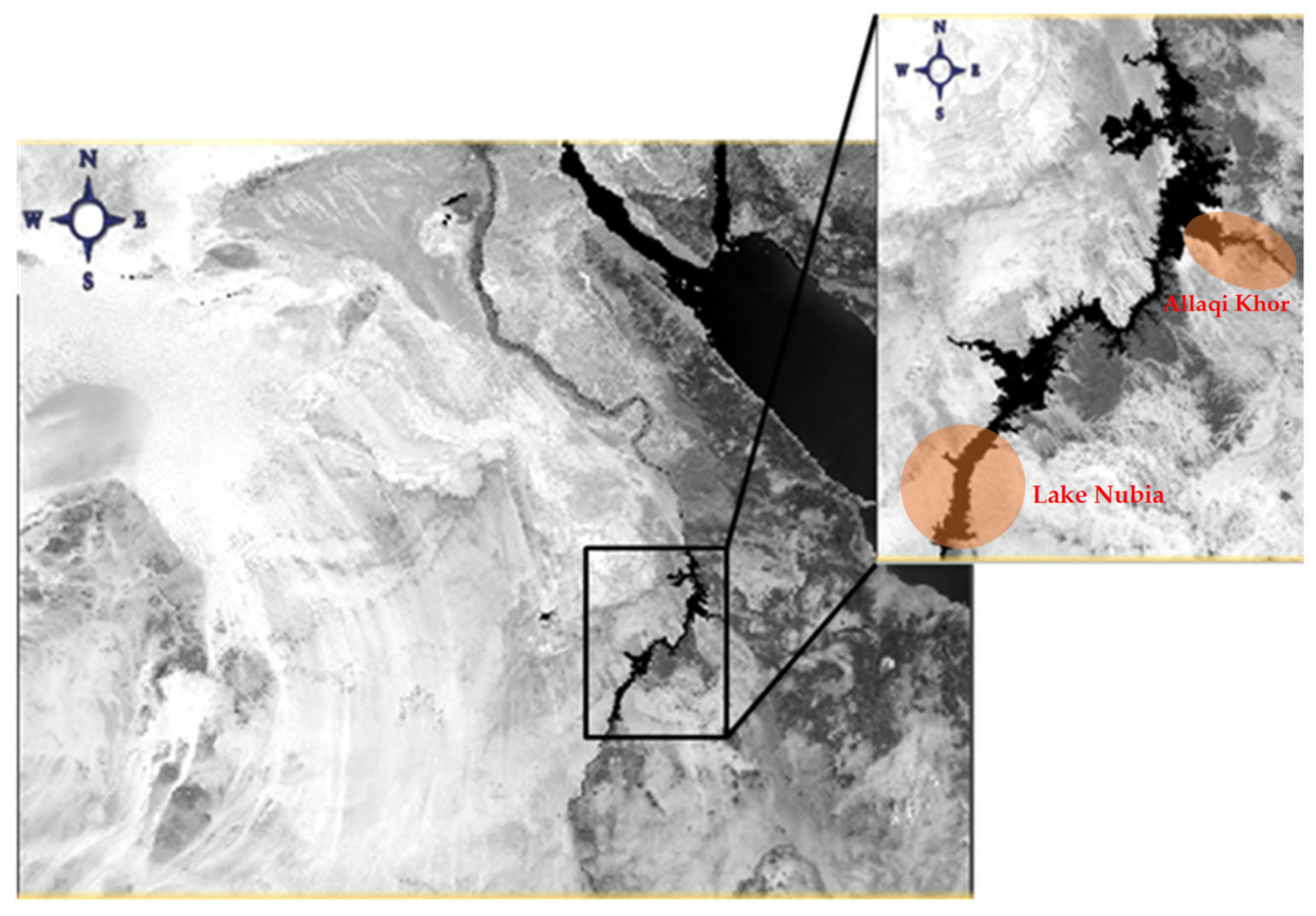
AHDL is the second largest man-made lake in the world. It was formed after the construction of the Aswan High Dam (AHD) in 1971 on the Nile River. It extends about 350 km in the southern part of Aswan (Egypt). It is named Lake Nasser (after Egypt’s president Gamal Abdel-Nasser). The second part of AHD is called Lake Nubia, stretching about 170 km towards in the North of Sudan. The water level ranges from 147 to 182 m above Mean Sea Level (MSL). The surface area of AHDL is variable due to the annual amount of flood entering the lake and the water discharges from it. When the High Dam is nearly full, with a water level of 180 m, the lake surface area could exceed 6276 km2 [28] and the mean depth of the reservoir is 25 m, while the maximum depth reaches up to 110 m at water level of 182 m above MSL. The lake is about 35 km large at its widest point, with a mean width about 10 km, and has a storage capacity of some 164 Billion Cubic Meters (BCM). The geographic boundary is between latitude 21° and 24°30’ north and longitude 31°30’ and 33° east [29], with a shoreline of more than 7800 km in length [30]. The shoreline of the AHDL has numerous embayments which are called Khors. Allaqi Khor is a secondary canal located approximately at 110 km from the upper stream of Aswan High Dam (AHD) on the eastern side of the lake, the depth was greater than 45m. This secondary canal stretches for about 75 km in length. It has a surface area of 500 km² with the largest water storage at 9.76 BCM [31].
3. Data Sets
3.1. Field Data
Two sources originate field data used in this research: the first data type used in this study was collected in a field survey trip in September 2018 with a bathymetric campaign based on a Multi Beam Echo Sounder, focused on the southern part of AHDL (named Lake Nubia), and another field survey trip for Allaqi Khor was in September 2013 (Figure 1). The Multi Beam Echo Sounder is a device that measures the bed levels by transmitting sound pulses into water (Figure 2). The natures of the water stream bed (underwater topography) were obtained from personal communication with the Nile Research Institute (NRI) [32] and with the Ministry of Agriculture and Land Reclamation (MALR), Egypt [33]. It is very difficult to obtain field data from these parties, and due to the difficulty of obtaining and publishing data, the bed levels of Allaqi Khor in 2013 were used to the case study in 2018 after being confirmed by Elsahabi [34] that the bed level is relatively stable due to the stability of the amount of sedimentation and erosion. In addition, the water level difference between the two periods was taken into account.
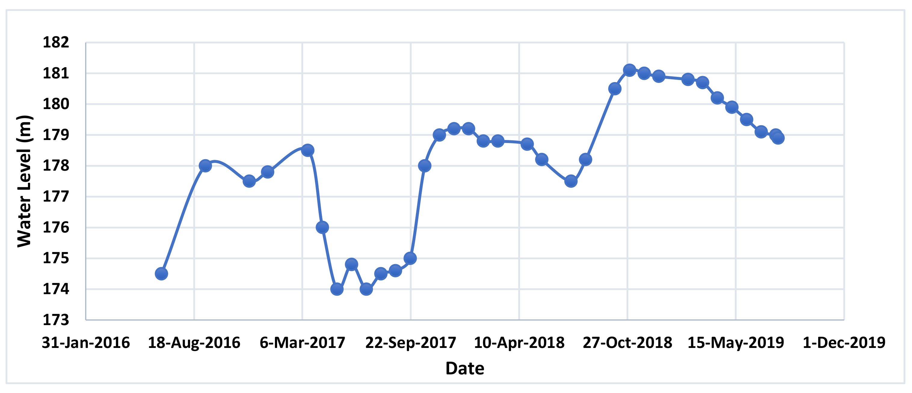
The second data type consisted of daily water level measurements between June 2016 and September 2019 at one gauging station for AHDL. Data were obtained from the Nile Research Institute (NRI) database for assessment. (Figure 3) shows measured water levels’ variation for time interval between 2016 and 2019.
3.2. Optical Images
All satellite images of Sentinel-3 data are available from The European Space Agency Copernicus Open Access Hub (ESA SciHub) [35], which is free to the public. We selected imaging products regarding AHDL in the mentioned time interval (2016 to 2019). Selected products were at processing level L1A. All the data relate to the relative orbit #249 (diurnal), crossing the AHDL for both instruments SLSTR and OLCI.
The moderate spatial resolution is useful for our study area to achieve full coverage of the AHDL in the same swath and relatively manageable memory occupation. The moderate spatial resolution is compensated for by a high radiometric performance for both instruments in terms of noise and quantization error [36], which is fundamental for experimenting on the retrieval of depth from optical measurements. In particular, we used the reflectance of green, red, and NIR bands for both SLSTR and OLCI instruments to estimate the lake’s depth. (Table 1) shows the main specifications of the two instruments, and (Table 2) lists the spectral bands used in this paper [4].
3.3. Altimetry Data
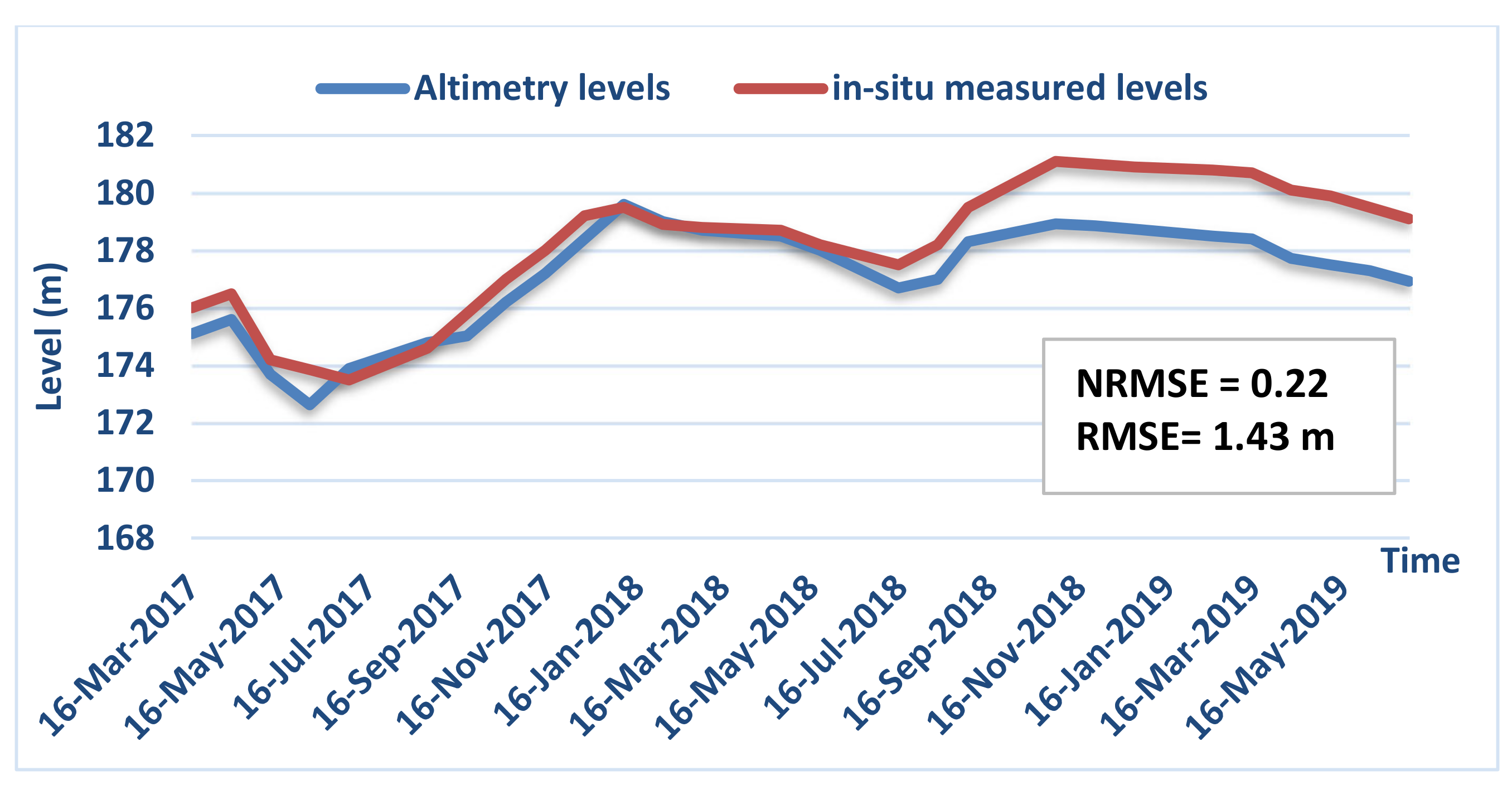
SRAL is the instrument that (hosted by Sentinel-3 satellite) we used for generating the water level time series in this paper. AHDL surface water level time series can be used as an input to Heron’s algorithm to estimate water volume variations in AHDL. The SRAL is a versatile altimeter working with a carrier frequency in the Ku-band (20 GHz) and a chirp (the wave shape of the transmitted signal) band width of 350 MHz. Substantially, the instrument is a nadir-pointing SAR (Synthetic Aperture Radar). Data used in this paper were processed by the ESA GPOD service (Grid Processing on Demand), running the SARvatore processor (SAR Versatile Altimetry Toolkit for Ocean Research and Exploitation). Water levels with respect to the earth reference ellipsoid were calculated with the aid of the SARvatore processor. The nominal track of the relative orbit #249 of Sentinel-3A is shown in (Figure 4), together with the ground projections of the actual measurement points. Water levels have been calculated in terms of “orbit-range” with no corrections, and were taken by the output (L2 level) product of SARvatore. A comparison between in situ water level time series and those of altimetry must be evaluated to check the precision of altimetry measurements, thus the possibility of calibrating altimetry measurements properly. In (Figure 5), both time series are plotted, showing a RMSE = 38 cm. We also demonstrated [37], that the simultaneous acquisition by optical imaging radiometers and SRAL offers the opportunity to cross-calibrate radiometric imagers as “optical altimeters” by estimating the percent coverage of water in coastline pixels. In this paper, we build on the same altimetry dataset. It is worth mentioning that all data from altimetry and radiometric images have been acquired in the same date of day/month/year and same track #249.
4. Methodology
4.1. Water Depth Estimation
In this preliminary study, we investigated the relationship between the reflectance of optical imagery from two instruments, SLSTR and OLCI instruments, hosted by the Sentinel-3A platform and in situ water depth data. Figure 6 present a short summary of the working methodology.
Sentinel-3A platform and in situ water depth data of AHDL offers an opportunity to experiment with empirical algorithms to estimate depth in deep water from optical radiometric measurements. For calibration and validation purposes, this activity is supported by water depth data from a field survey of the study area by echo sounding (SONAR). Figure 2d presents the spatial position of the Nubia Lake dataset that was used to build the bathymetry model (45 points) and the spatial position of the Allaqi Khor dataset that was used to validate the model (22 points). We used correlation techniques between field data and the reflectance of optical imagery for estimating various parameters. The transformation from radiance to reflectance of all bands for both OLCI and SLSTR was carried out with the SNAP software. Spatially co-located depth values were obtained by GIS software. While the scatter analysis of reflectance vs. the true measured water depth was made by MS Excel. The developed relationship between spectral reflectance and depth was a simple regression model based on a polynomial equation of 2nd degree with coefficient of determination > 0.8, which highlights a good relationship between the reflectance and measured field.
4.2. Water Surface Area Estimation
Unsupervised classifications were performed on masked scenes to identify significant patterns in the images. While unsupervised k-means classification was performed by using the SNAP software of Sentinels Scientific Data Hub on creating our data subset that were clipped from the footprint images to extract the study area of SLSTR for period June 2016 to September 2019. The NIR band has been used to mask the land area from the image. The resulting unsupervised classified images showed different classes according to the class number assigned, as the water appears dark and has sharp edges discriminating water from land, which looks relatively bright (Figure 7).
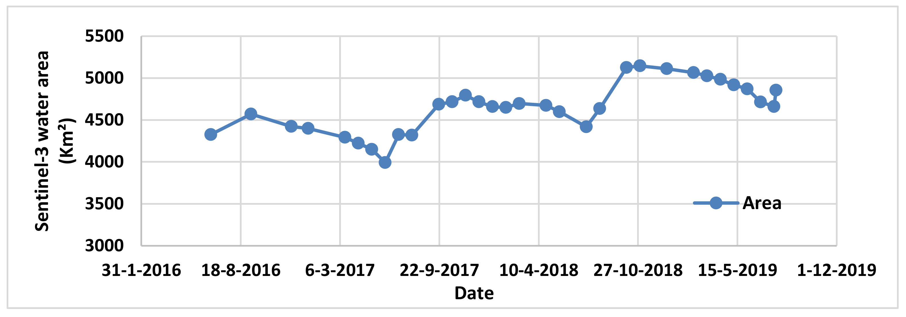
The resulting classification images were opened in QGIS to extract water surface from the image using a raster calculator and mask land area from the images. Figure 8 shows the estimated water surface area of whole AHDL for all-time series. There is no atmospheric correction applied because AHDL is considered to have zero cloud cover, and the atmospheric path delays and extinction are considered constant.
4.3. Water Volume Variations
A combination of satellite products was used to estimate the change in the lake volume from both the variation in the water level and the surface area. This is an empirical relationship between the lake surface (that can be derived from optical images) and water levels (that can be derived from satellite radar altimetry). The volume of a pyramidal frustum was derived 2000 years ago by the Greek mathematician Heron, native of Alexandria (10–70 AD), as follows:
where L1 and L2 are two water levels with corresponding surface areas. A1 and A2 denote the difference in the water levels and the volume between two dates t1 and t2, respectively [38]. This is still the basic formula used by limnologists to estimate the volume of lakes since 2000 years ago. To this end, the lake of interest can be modeled as a simple geometric shape, for which the variation in the water volume (ΔV) between two dates (t1 and t2, respectively) depends on L1 and L2 values taken from altimetry data or in situ gauges; A1 and A2 can be computed as described in Section 4.2. Equation (1) is applicable when the area increases linearly with change in water level; this assumption is valid for small intervals in water level but is not necessarily true over large changes in water level [26].
5. Results and Discussion
5.1. Water Depth Estimation
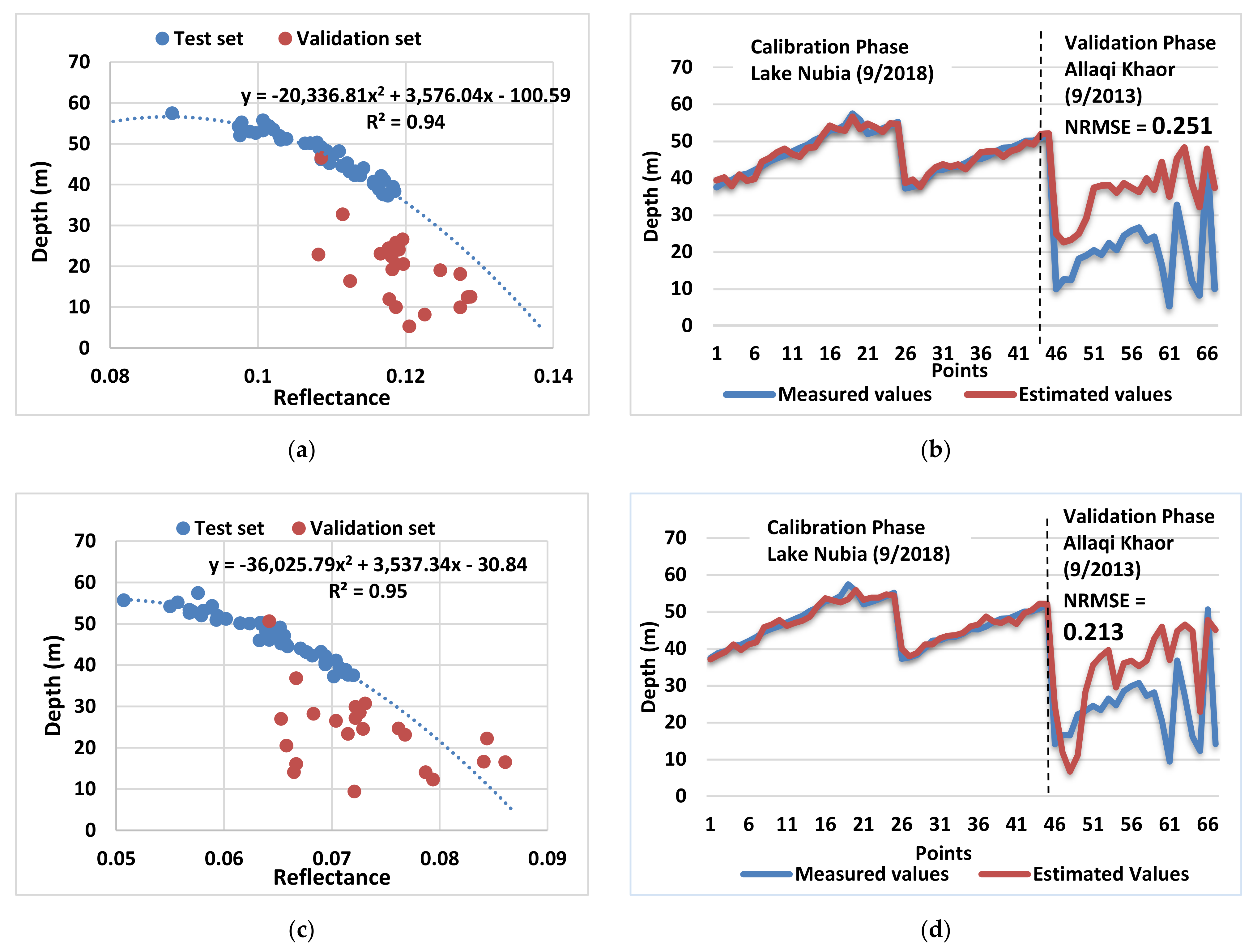
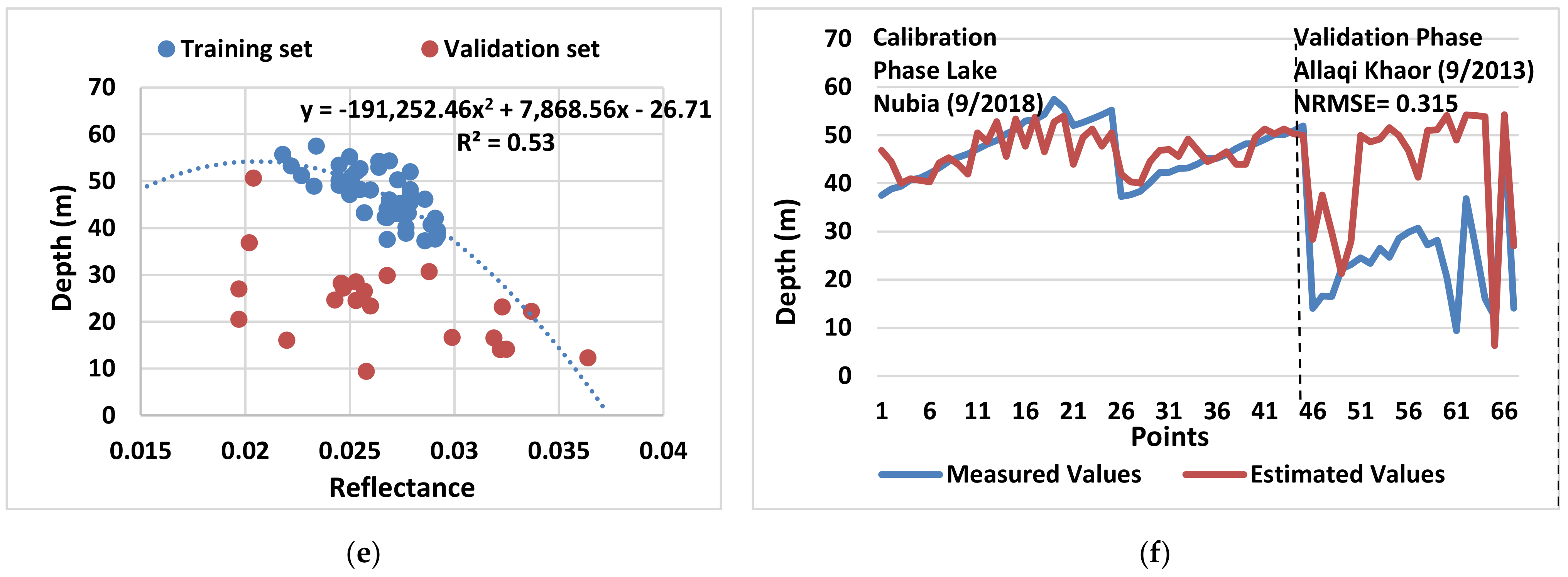
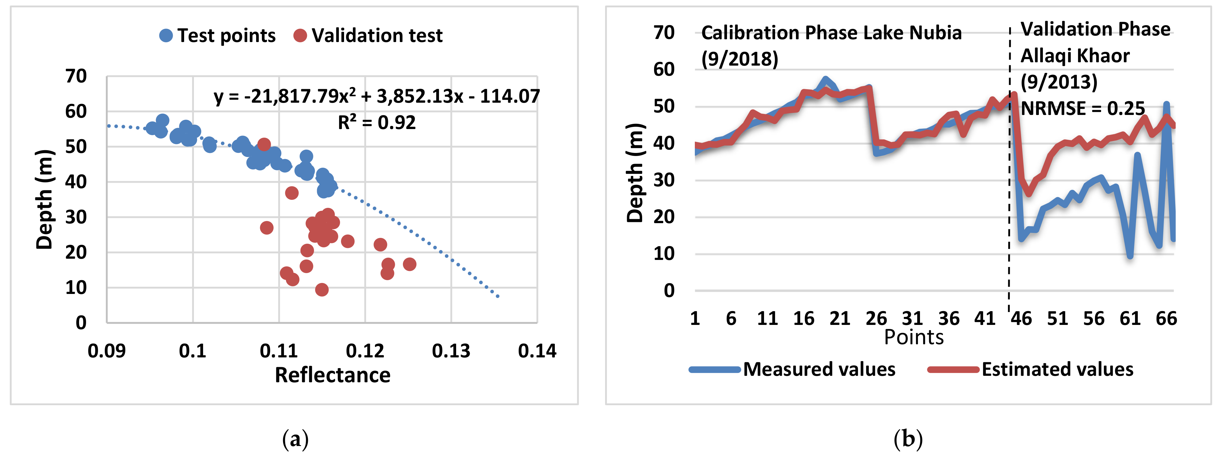
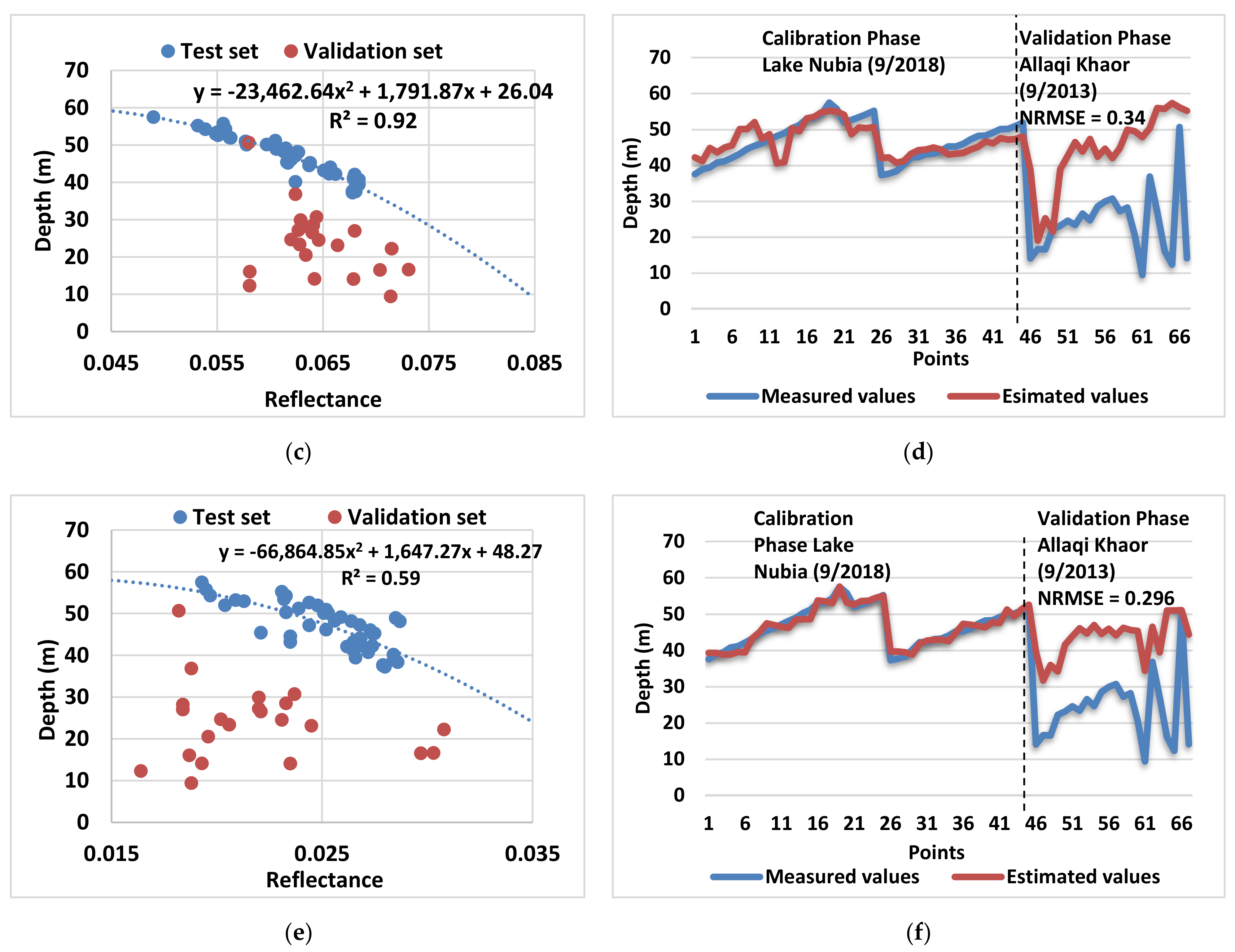
The correlation between the reflectance of all the three bands, green, red, and NIR, for both SLSTR and OLCI with in situ measured depth is presented in (Figure 9 and Figure 10). The datasets were selected relatively far from the edges of the Nubia lake shore and Allaki Khor shore with the aim of avoiding coastal pixels due to the spatial resolution of the imaging sensors. The spatial position of the Nubia Lake dataset was used to build a simple model based on a quadratic equation in the calibration phase. Those points were called “test set” and their number was 45 points, while the spatial position of 22 points assigned to the Khor Allaqi dataset, represented the model’s validity relationship between in situ measured depth and corresponding reflectance from green, red, and NIR band for SLSTR and OLCI instruments in the validation phase; those points are called the “Validation set”. The spatial position of all 67 points was from the Sentinel-3 satellite image on 21 September 2018 of Lake Nubia data and 27 September 2013 of Allaqi Khor data, as well as the water level used to estimate the depth, on the same Lake Nubia data date.
Transformation from radiance to reflectance of all bands for both OLCI and SLSTR was carried out with the SNAP software. The three bands, green, red, and NIR, of two instruments SLSTR and OLCI, hosted by the Sentinel-3A platform, were used to make preliminary study for investigating the relationship between optical measurements (i.e., reflectance, in our case) and in situ measured water depth data. The correlation between in situ depth measurements and the corresponding reflectance values for each band was determined and their relationship could be approximated by a quadratic equation. The green band resulted in a slightly higher accuracy than the red band; R2 of the green band is equal to 0.93 for the SLSTR instrument and 0.92 for the OLCI instrument, while R2 in the red band is equal to 0.95 and 0.92 for SLSTR and OLCI, respectively. The NIR band is characterized by a much lower accuracy of the model (R2 = 0.53 for SLSTR instruments and R2 = 0.59 for OLCI instruments). Armstrong [15] estimated water depth from decades of radiometry images by bottom albedo signal where it successfully retrieved depth values with a coefficient of determination R2 of 0.70 for a deep depth range to 20 m. The RMSE is equal to 10.15 m, 10.55 m, and 15.02 m for green, red, and NIR bands, respectively, of the SLSTR instrument, and NRMSE with in situ measured depths of Allaqi Khor which was used to validate the model is equal to 0.251, 0.213, and 0.315 of green, red, and NIR bands, respectively, while RMSE of the OLCI instrument bands is equal to 11.96 m, 14.5 m, and 16 m for green, red, and NIR bands, respectively, and NRMSE with in situ measured depths of Allaqi Khor is equal to 0.25, 0.34, and 0.296 of green, red, and NIR bands, respectively. Reflectance of the band with higher absorption (green) will decrease with increasing depth relatively faster than reflectance of the band with lower absorption (NIR), because the green and red bands have a good penetration in the water column [14]. The NIR band of the spectrum attenuates more rapidly than the shorter wave length in the visible region, and the green band was found more significant for depth derivation. The promising results obtained in terms of correlation indicate a good relationship between the measured reflectance and depth.
5.2. Water Surface Estimation
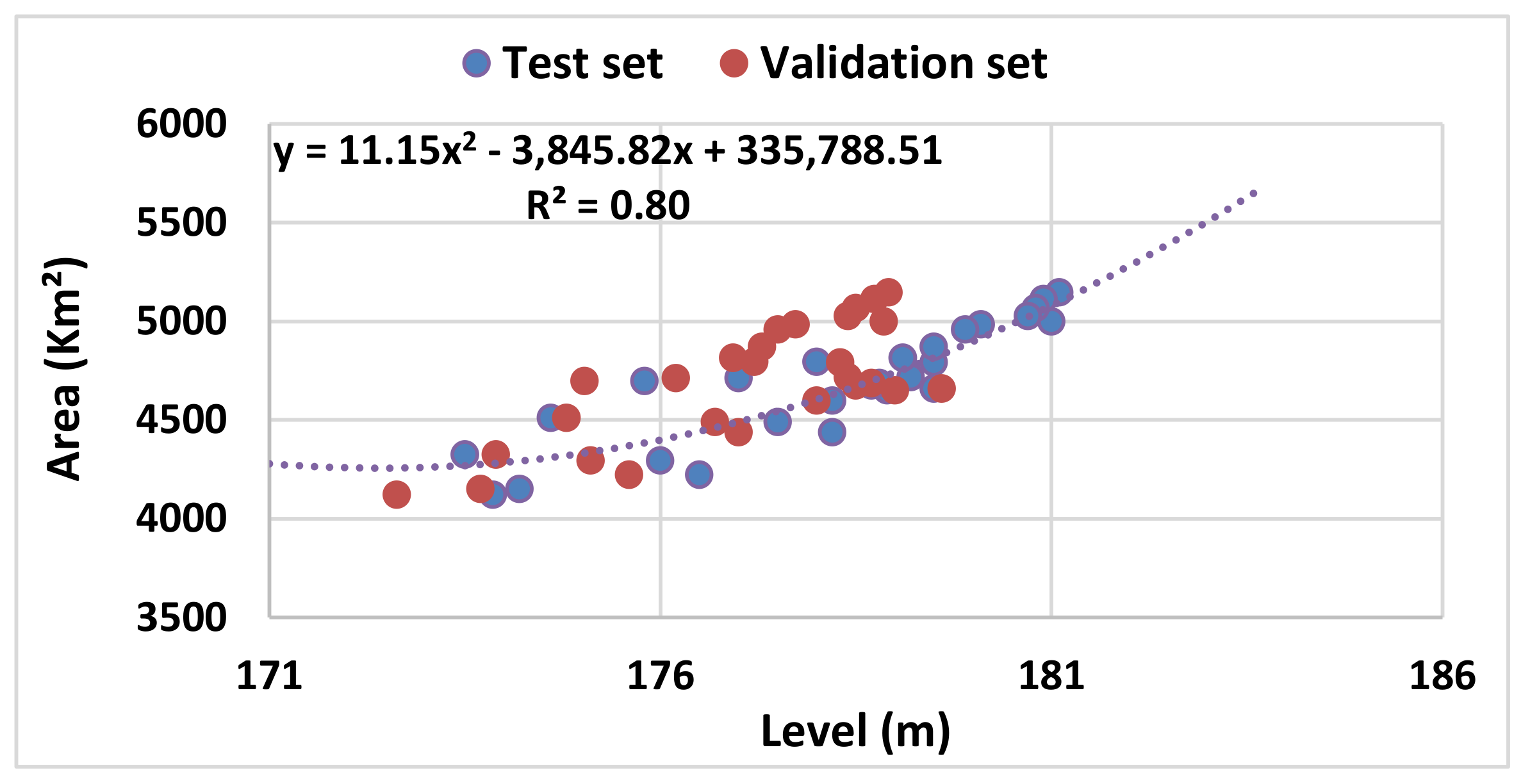
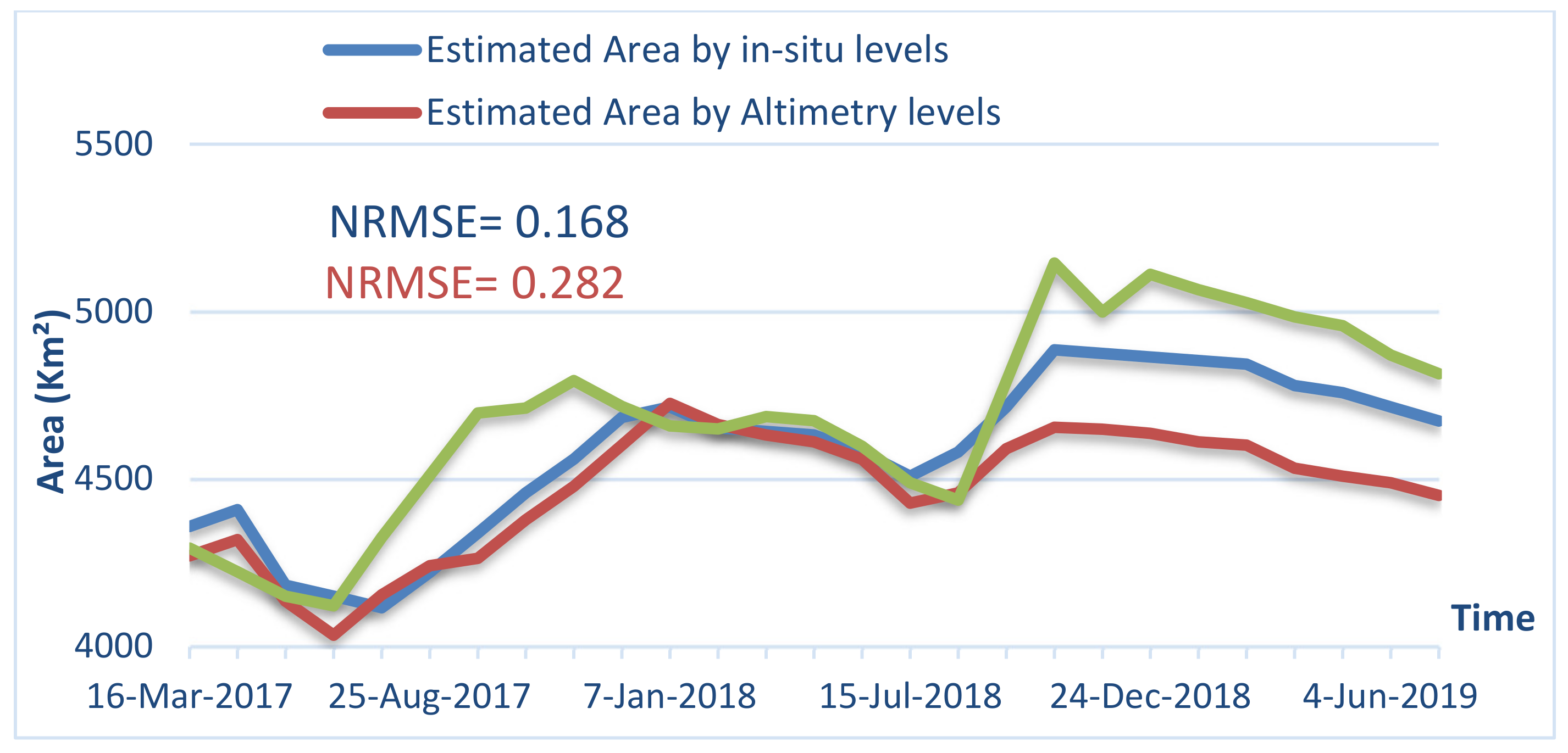
Figure 11 shows the relationship between surface area (in km2) extracted from SLSTR images in the NIR band during the period from June 2016 to July 2019, and: (i) radar altimetry, which is called a “calibration dataset” that represents the relationship between area and level in meters via a quadratic polynomial equation with correlation coefficient equal to 0.81 and (ii) in situ water levels. Validation of the model results was made with the aid of in situ water levels in blue points which called “validation dataset”. The accuracy of the model is evaluated using simple statistical parameters, such as the coefficient of determination R2, which represents the relationship between the AHDL area estimated unsupervised method in Section 4.2 and between the altimeter level. The second parameter used normalized root mean square errors (NRMSE) to measure errors of this simple regression model, as shown in (Figure 12). The curves represent the changes of area over time, the blue curve represents surface area estimated by the model based on in situ measured water level with NRMSE equal to 0.168, the red curve represents surface area estimated by the model based on Sentinel-3 altimetry water level with NRMSE equal to 0.282. Water surface area was estimated by the unsupervised method of Sentinel-3 optical images stimulated by green curve during the period time. These values give us confidence in the extract water surface areas from this simple regression model and the optical satellite images with Sentinel-3 of 300 m resolution. Fawzy [39] used this simple regression model to describe the relation between surface area and level for Klabsha and Allaqi Khors with a second order polynomial equation and resulting correlation coefficient from the equation equal to 0.99. Ablieh [26] used radar altimetry technique with radiometer imagery over AHD Lake’s specific area-level relationship for the periods from 1999 to 2002 and 2005 to 2009 was found with correlation coefficient R2 = 0.9985.
5.3. Water Volume Variations
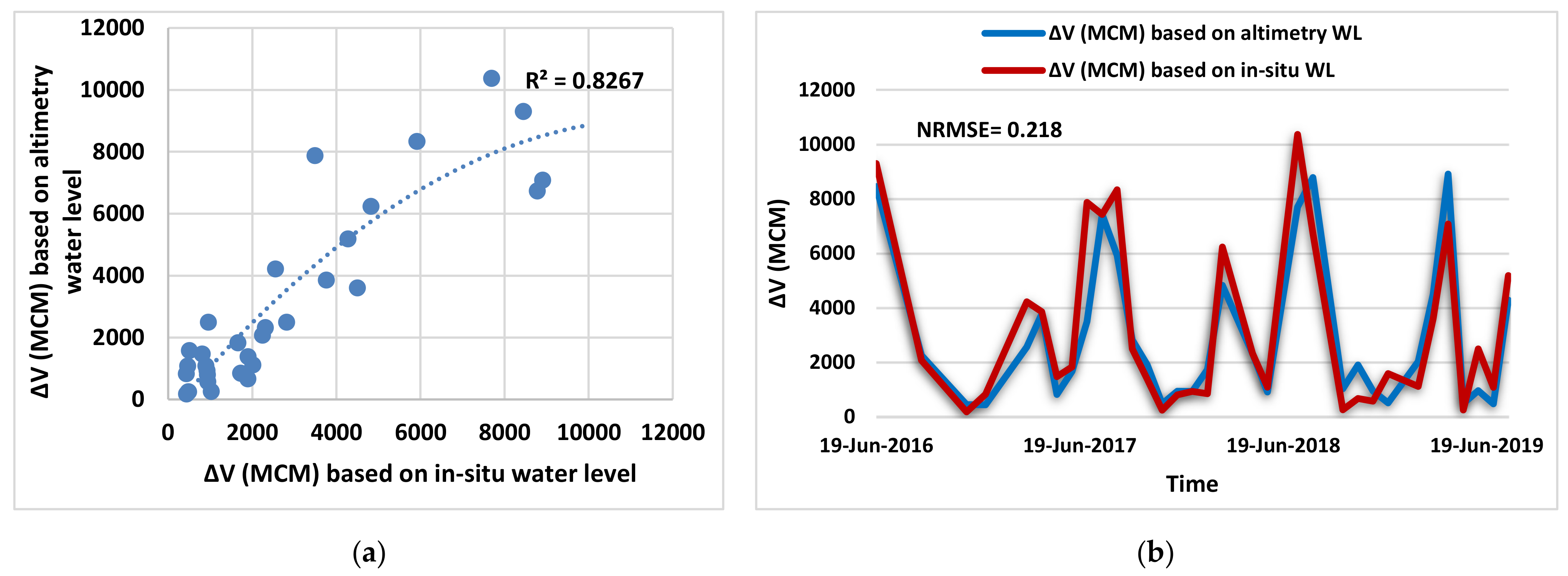
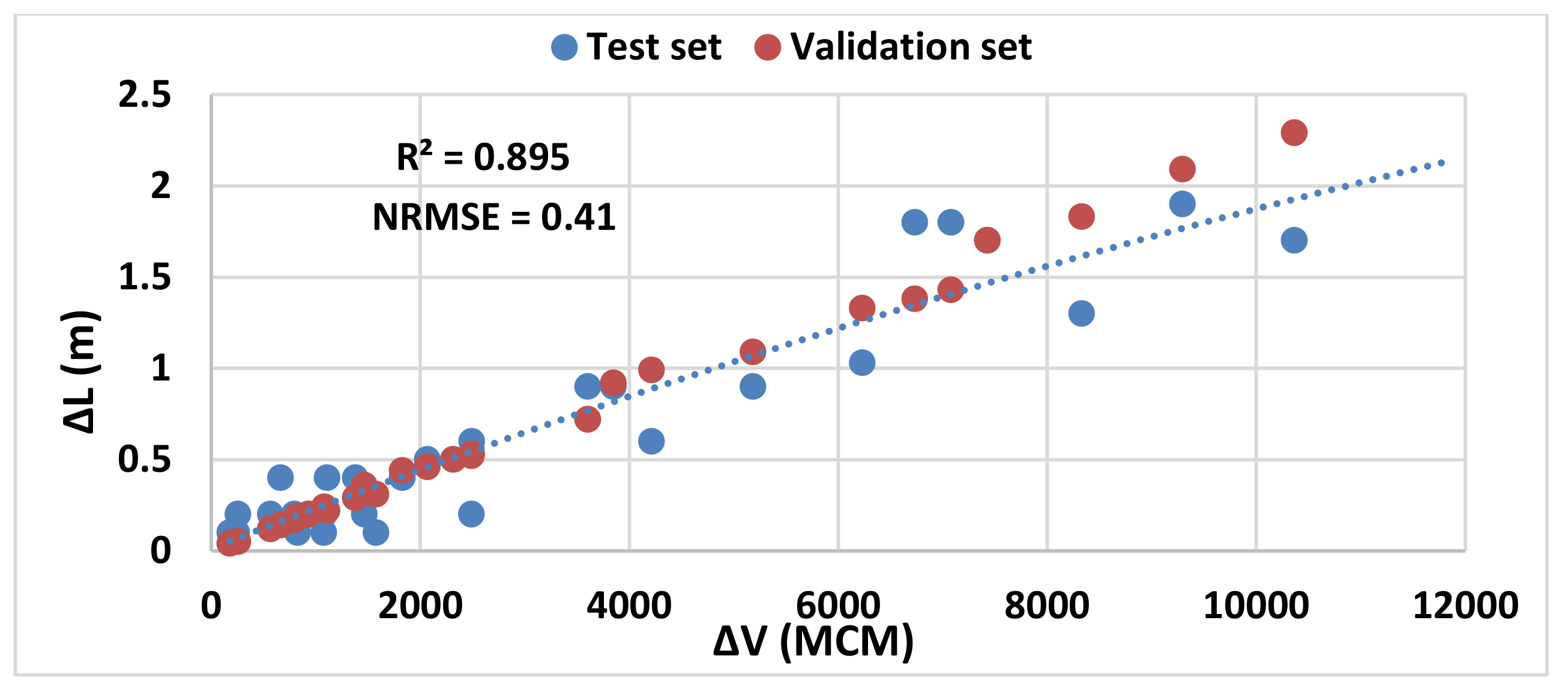
Figure 13 shows the results of estimating water volume variations (∆V) by applying Heron’s formula in Equation (1), based on altimetry water levels and surface areas estimated by satellite images. Validation of the results was made with the aid of in situ water levels. (Figure 13a) shows a scatter plot of the measured ∆V in million cubic meters (MCM) based on altimetry and ∆V based on in situ water levels, and presented the water volume variations above the lowest reference water level. A second order polynomial fitting is plotted in the same figure, and a correlation coefficient R2 = 0.83. An NRMSE value of approximately 12.8% was presented (Figure 13b), and also shows water volume variations over a time period from June 2016 to July 2019. The results are relatively similar to the results of Ebaid [27], who also applied the Heron method for the period from 2014 to 2015 to estimate water volume variations relative to reference water level for the southern part of AHDL in Egypt. She used available free Landsat and radar altimeter datasets with R2 = 0.98 and RMSE values that were 13.2% of the mean volume variation. The (ΔV versus ΔL) relationship in (Figure 14) shows the radar altimetry water levels and the volume variation estimate by Heron’s method (ΔV) during the same period of the previous plot. This is called “Test dataset”. A second order polynomial fitting exhibits a correlation coefficient R2 = 0.89.
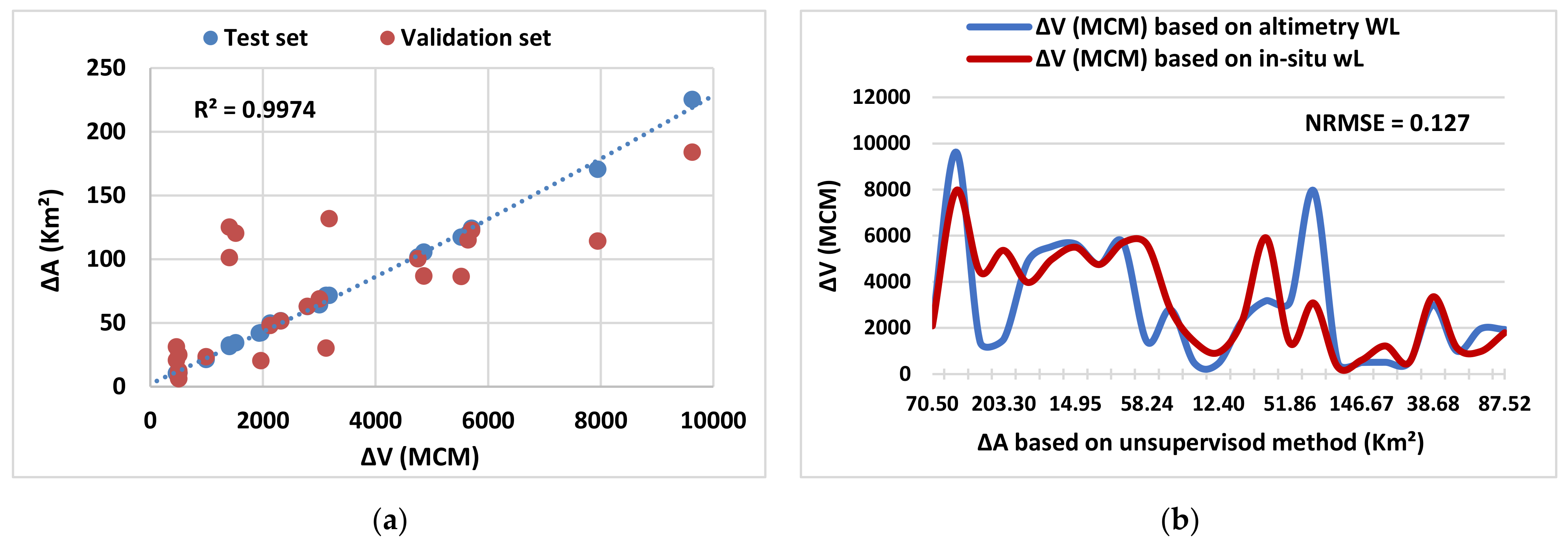
The (ΔV) and (ΔA) relationship in (Figure 15a) shows the variation in water area (ΔA) estimated in Section 5.2 with volume variation estimated by Heron’s method (ΔV) estimated in Section 5.3, and the “Test dataset” represented the ΔV estimated by the radar altimetry water levels again during the same period. In this case, a 2nd order polynomial fitting exhibits an R2 = 0.55, the “Validation dataset” represented the ΔV estimated by the in situ measured levels with NRMSE value 12.8% over the same time period, as shown in (Figure 15b). In addition, the validation of the studies carried out at Lake Mead in U.S.A by [40], Lake IJsselin in the Netherlands, and Lake Tanain in Ethiopia to estimated water volumes of all lakes agreed well with in situ water level R2 ranged from 0.95 to 0.99, and the RMSE was within 4.6 to 13.1% of the mean volumes of in situ measurements, which is consistent with the estimation results of this study on AHDL.
The accuracy of ΔV affected by the relation between water levels and corresponding surface areas, as when water levels increase, the volume variations estimated from Heron methods will increase. Moreover, the surface area deduced from satellite images will increase especially at boundary regions more than the middle stream of the lake, which may cause unreal water volume variations at the lake [31]. The high-water levels may cause errors in estimation of volume variation by applying the 2nd order polynomial relationship between water levels’ variation and volume variation (Figure 14) or between surface areas’ variation and volume variation (Figure 15). The errors also increase with the irregularity of the time period between the variables of the Heron equation, meaning that the duration between two water levels or the water surface must have been regular sequentially, but that is difficult for limited free images clear of cloud over the lake and in situ data measured, obtained from (NRI) [32].
6. Conclusions
This paper investigates techniques based on optical and radar sensing for the retrieval of depth, area, and volume variations in a surface water body. AHDL, one of the most challenging hot spots at both local and global levels, was chosen as a case study to apply the proposed methodology. We determined water depth, surface area, and volume variations over the time series variation in AHDL. For what concerns water depth, we experimented with a combination of optical Sentinel-3 imagery data in the green, red, and NIR bands for both instruments, SLSTR and OLCI, with field survey bathymetric data of Nubia Lake and Allaqi Khor (parts of AHDL). The developed relationship between spectral reflectance and depth was a simple regression model based on a polynomial equation, describing the functional relationship between the optical measurement and the corresponding depth. Promising correlation values were obtained, R2 > 0.8 and NRMSE < 0.4. Additionally, we explored the possible use of the combination of optical imagery and Sentinel-3 altimetry water level to estimate water storage variations in AHDL by using Heron’s algorithm. The developed model has R2 = 0.83 and NRMSE = 0.128. Similarly, the lake’s surface area in relationship with the depth was explored. Preliminary results for AHDL, shown in this paper, represent a promising experience for monitoring the change in depth, area, and volume of AHDL water. Further tests are needed to firmly demonstrate these techniques in order to enhance accuracy. In addition, further improvements are expected when integrating additional data from current and future satellite missions to generalize the relationship model to be valid for all geographic regions of AHDL. We recommend the use of Sentinel-3 satellite data with its moderate resolution to calculate the bathymetric properties of large lakes, but the methodology still needs calibration and verification using large datasets on different lakes for a final confirmation. Additionally, smaller water bodies and rivers may require a higher spatial resolution, suggesting the usage of other missions, such as Sentinel-2. Moreover, and in general, the application of generalizable models leads to a better understanding of their potentialities, for deep water lakes and inland water. Furthermore, improved integration between deduced data from field survey and remote sensing data, such as limnology, hydrology, and ecology, leads to a wider usage of remote sensing models in scientific studies of management water resources.
Author Contributions
H.H., M.K., A.S., A.N. and M.E. shared their thoughts to formulate the idea. M.K. applied the methodology and drafted the first version of the manuscript. H.H. and M.E. supervised M.K during the phases of applying the methodology and writing the first draft of the manuscript. Both A.S. and A.N. provided their comments and revisions until the submission phase of the manuscript. H.H., S.G. and M.E. supervised M.K. during the implementation of the comments and revisions. All authors have read and agreed to the published version of the manuscript.
Funding
This research work received funding from Academy of Scientific Research and Technology (ASRT) of Egypt and the Italian National Research Council (CNR) in the framework of the bilateral CNR-ASRT mobility project titled “Experimentation of the new Sentinel missions for the observation of inland water bodies on the course of the Nile River”.
Institutional Review Board Statement
Not applicable.
Informed Consent Statement
Not applicable.
Data Availability Statement
All data generated or analyzed during this study are included in this published article. The satellite images and altimetry data provision is available to all users via the Sentinel Data Hub https://scihub.copernicus.eu/ accessed on 13 Decembar 2021. Here, you can download the latest installers for SNAP and the Sentinel Toolboxes: https://step.esa.int/main/toolboxes/snap/ accessed on 13 Decembar 2021. Here, you can download the latest installers for https://www.qgis.org/en/site/ accessed on 13 Decembar 2021.
Acknowledgments
The authors acknowledge the financial support from the Academy of Scientific Research and Technology (ASRT) of Egypt and the Italian National Research Council (CNR) via the bilateral CNR-ASRT project titled “Experimentation of the new Sentinel missions for the observation of inland water bodies on the course of the Nile River”.
Conflicts of Interest
The authors declare no conflict of interest.
References
- Mishra, D.R.; Gould, R.W. Preface: Remote sensing in coastal environments. Remote Sens. 2016, 8, 665. [Google Scholar] [CrossRef] [Green Version]
- Sánchez-Carneroab, N.; Ojeda-Zujarb, J.; Rodríguez-Pérezc, D.; Marquez-Perezb, J. Retrieval of near shore bathymetry from Landsat 8 images: A tool for coastal monitoring in shallow waters. Remote Sens. Environ. 2015, 159, 102–116. [Google Scholar]
- Hamed, M.A. Estimation of water quality parameters in Lake AHD using remote sensing techniques. In Proceedings of the Twentieth International Water Technology Conference, IWTC20, Hurghada, Egypt, 18–20 May 2017. [Google Scholar]
- European Space Agency (ESA). Technical-Guides 2020. Available online: https://sentinel.esa.int/web/sentinel/sentinel-technical-guides (accessed on 20 February 2020).
- Topp, S.N.; Pavelsky, T.M.; Jensen, D.; Simard, M.; Ross, M.R.V. Research trends in the use of remote sensing for inland water quality science: Moving towards multidisciplinary applications. Water 2020, 12, 169. [Google Scholar] [CrossRef] [Green Version]
- Maheswari, R.U. Mapping the Under Water Habitat Related to their Bathymetry using Worldview-2 (wv-2) Coastal, Yellow, Rededge, Nir-2 Satellite Imagery in Gulf of Mannar to Conserve the Marine Resource. Int. J. Mar. Sci. 2013, 3, 91–97. [Google Scholar] [CrossRef] [Green Version]
- El-Askary, H.; Abd El-Mawla, S.H.; Li, J.; El-Hattab, M.M.; El-Raey, M. Change detection of coral reef habitat using Landsat-5 TM, Landsat 7 ETM+ and Landsat 8 OLI data in the Red Sea (Hurghada, Egypt). Int. J. Remote Sens. 2014, 35, 2327–2346. [Google Scholar] [CrossRef]
- Jawak, S.D.; Luis, A.J. Spectral information analysis for the semiautomatic derivation of shallow Lake bathymetry using high-resolution multispectral imagery: A case study of Antarctic coastal oasis. Aquat. Procedia 2015, 4, 1331–1338. [Google Scholar] [CrossRef]
- Hafizt, M.; Manessa, M.D.M.; Adi, N.S.; Prayudha, B. Benthic habitat mapping by combining Lyzenga’s optical model and relative water depth model in Lintea Island, Southeast Sulawesi. IOP Conf. Ser. Earth Environ. Sci. 2017, 98, 012037. [Google Scholar] [CrossRef] [Green Version]
- Geyman, E.C.; Maloof, A.C. A simple method for extracting water depth from multispectral satellite imagery in regions of variable bottom type. Earth Space Sci. 2019, 6, 527–537. [Google Scholar] [CrossRef]
- Lyzenga, D.R. Passive remote sensing techniques for mapping water depth and bottom features. Appl. Opt. 1978, 17, 379–383. [Google Scholar] [CrossRef]
- Stumpf, R.P.; Holderied, K.; Sinclair, M. Determination of water depth with high-resolution satellite imagery over variable bottom types. Limnol. Oceanogr. 2003, 48, 547–556. [Google Scholar] [CrossRef]
- Mumby, P.J.; Clark, C.D.; Green, E.P.; Edwards, A.J. Benefits of water column correction and contextual editing for mapping coral reefs. Int. J. Remote Sens. 1998, 19, 203–210. [Google Scholar] [CrossRef]
- Manessa, M.D.M.; Kanno, A.; Sekine, M.; Ampou, E.E.; Widagti, N.; Assyakur, A.R. Shallow-water benthic identification using multispectral satellite imagery: Investigation on the effects of improving noise correction method and spectral cover. Remote Sens. 2014, 6, 4454–4472. [Google Scholar] [CrossRef] [Green Version]
- Hernandez, W.J.; Armstrong, R.A. Deriving bathymetry from multispectral remote sensing data. J. Mar. Sci. Eng. 2016, 4, 8. [Google Scholar] [CrossRef]
- Mostafa, M.M.; Soussa, H.K. Monitoring of Lake AHD Using Remote Sensing: From Pixels to Processes; ITC Faculty Geo-Information Science and Earth Observation: Enschede, The Netherlands, 2006; pp. 8–11. [Google Scholar]
- Jerlov, N.G. Optical classification of ocean water. In Physical Aspects of Light in the Sea; University Hawaii Press: Honolulu, HI, USA, 1964; pp. 45–49. [Google Scholar]
- Green, E.P.; Mumby, P.J.; Edwards, A.J.; Clark, C.D. Remote Sensing Handbook for Tropical Coastal Management; Edwards, A.J., Ed.; UNESCO: Paris, France, 2000. [Google Scholar]
- Jerlov, N.G. Optical Studies of Ocean Water. In Reports of Swedish Deep-Sea Expedition; Elanders Boktryckeri Aktiebolag: Mölnlycke, Sweden, 1951; pp. 73–97. [Google Scholar]
- Spitzer, D.; Dirks, R.W.J. Bottom influence on the reflectance of the sea. Int. J. Remote Sens. 1987, 8, 279–290. [Google Scholar] [CrossRef]
- Birkett, C.M. The contribution of Topex/Poseidon to the global monitoring of climatically sensitive Lakes. J. Geophys. Remote Sens. Environ. 1995, 100, 25179–25204. [Google Scholar] [CrossRef]
- Cazenave, A.; Bonnefond, P.; Do Minh, K. Caspian Sea level from Topex/Poseidon altimetry: Level now falling. Surv. Geophys. 1997, 25, 155–158. [Google Scholar] [CrossRef]
- Crétaux, J.F.; Jelinski, W.; Calmant, S.; Kouraev, A.; Vuglinski, V.; Bergé Nguyen, M.; Gennero, M.C.; Nino, F.; Del Rio, R.A.; Cazenave, A.; et al. SOLS: A Lake database to monitor in the Near Real Time water level and storage variations from remote sensing data. Adv. Space Res. 2011, 47, 1497–1507. [Google Scholar] [CrossRef]
- Muala, E.; Mohamed, Y.A.; Duan, Z.; Van der Zaag, P. Estimation of reservoir discharges from Lake AHD and Roseires Reservoir in the Nile Basin using satellite altimetry and imagery data. Remote Sens. 2014, 6, 7522–7545. [Google Scholar] [CrossRef] [Green Version]
- Shafik, N.M. Updating the Surface Area and Volume Equations of Lake AHD, using Multi Beam System. In Proceedings of the 19th International Water Technology Conference, Sharm El Sheikh, Egypt, 21–23 April 2016. [Google Scholar]
- Abileah, R.; Vignudelli, S.; Scozzari, A. A completely remote sensing approach to monitoring reservoirs water volume. Int. Water Technol. 2011, 1, 63–77. [Google Scholar]
- Ebaid, H.M.; Aziz, M. Integrating Radar Altimeters and Optical Imagery Data for Estimating Water Volume Variations in Lakes and Reservoirs (Case Study: Lake Nasser). J. Geogr. Inf. Syst. 2017, 9, 648–662. [Google Scholar] [CrossRef] [Green Version]
- Jeongkon, K.; Mohamed, S. Assessment of long-term hydrologic impacts of LakeAHD and related irrigation projects in Southwestern Egypt. Sci. J. Hydrol. 2002, 262, 68–83. [Google Scholar]
- Sadek, M.F.; Shahin, M.M.; Stigter, C.J. Evaporation from the reservoir of the high Aswan dam, Egypt: A new comparison of relevant methods with limited data. Theor. Appl. Climatol. 1997, 56, 57–66. [Google Scholar] [CrossRef]
- Hamdan, A.M.; Zaki, M. Long-term estimation of water losses through evaporation from water surfaces of AHD Lake Reservoir, Egypt. Int. J. Civ. Environ. Eng. 2016, 16, 13. [Google Scholar]
- Elba, E.; Farghaly, D. Modeling High Aswan Dam Reservoir Morphology Using Remote Sensing to Reduce Evaporation. Int. J. Geosci. 2014, 2014, 156–169. [Google Scholar] [CrossRef] [Green Version]
- NRI Nile Research Institute. Annual Report of Sedimentation in Lake Nubia—Wadi Halfa Field Trips (1973–2012); National Water Research Center: Cairo, Egypt, 2012; (No regular monitoring mission was conducted after 2012. However, limited monitoring was done and we succeeded to have some observations via personal communications and the reference documented the measurements tools/methods). [Google Scholar]
- MALR The Ministry of Agriculture and Land Reclamation, Egypt. The General Authority for AHDL Development, AHDL levels (1978 to 2010); The Ministry of Agriculture and Land Reclamation: Giza, Egypt, 2010.
- Negm, A.; Elsahabi, M.; Abdel-Fattah, S. Estimating the Sediment and Water Capacity in the Aswan High Dam Lake Using Remote Sensing and GIS Techniques. In The Nile River. Handbook of Environmental Chemistry; Springer: Berlin/Heidelberg, Germany, 2016. [Google Scholar] [CrossRef]
- European Space Agency (ESA). scihub. 2020. Available online: https://scihub.copernicus.eu/dhus/#/home (accessed on 15 January 2020).
- Coppo, P.; Mastrandrea, C.; Stagi, M.; Calamai, L.; Nieke, J. Sea and Land Surface Temperature Radiometer detection assembly design and performance. J. Appl. Remote Sens. 2014, 8, 084979. [Google Scholar] [CrossRef]
- Scozzari, A.; Vignudelli, S.; Negm, A. Lake water level estimated by a purely radiometric measurement: An experiment with the SLSTR radiometer onboard Sentinel-3 satellites. In Proceedings of the IEEE International Instrumentation and Measurement Technology Conference 2020 (I2MTC), Dubrovnik, Croatia, 25–28 May 2020; pp. 1–6. [Google Scholar]
- Taube, C.M. Instructions for winter Lake mapping. In Manual of Fisheries Survey Methods II: With Periodic Updates; Special Report N. 25; Schneider, J.C., Ed.; Department of Natural Resources, Fisheries: Lake Michigan, MI, USA, 2000; pp. 1–8. [Google Scholar]
- Fawzy, A.; Elbahrawy, A.; Sayed, E. Estimate of Hydrologic Characteristics of Major Khors in Lake Nasser. Al-Azhar Univ. Civ. Eng. Res. Mag. (CERM) 2019, 41, 2. [Google Scholar]
- Zheng, D.; Bastiaanssen, W.G.M. Estimating Water Volume Variations in Lakes and Reservoirs from Four Operational Satellite Altimetry Databases and Satellite Imagery Data. Remote. Sens.Environ. 2013, 134, 403–416. [Google Scholar]
Figure 1.
Aswan High Dam Lake, selected area shows Nubia Lake and Allaqi Khor, area clipped from Sentenel-3 image shows most of Egypt and the Red Sea in the footprint (image taken in October 2018).
Figure 1.
Aswan High Dam Lake, selected area shows Nubia Lake and Allaqi Khor, area clipped from Sentenel-3 image shows most of Egypt and the Red Sea in the footprint (image taken in October 2018).

Figure 2.
(a,b) show the use of new survey technology and the multi-beam echo sounder to determine the depth [25]; (c) shows paths of a bathymetric field trip in the study area, and (d) shows the locations of the bathymetry points used in building the bathymetry model.
Figure 2.
(a,b) show the use of new survey technology and the multi-beam echo sounder to determine the depth [25]; (c) shows paths of a bathymetric field trip in the study area, and (d) shows the locations of the bathymetry points used in building the bathymetry model.

Figure 3.
In situ water level of AHDL between 2016–2019 obtained from (NRI) [32].
Figure 3.
In situ water level of AHDL between 2016–2019 obtained from (NRI) [32].

Figure 4.
The nominal track of the relative orbit #249 of Sentinel-3A passes through AHDL.

Figure 5.
Difference between in situ measured water levels and Sentinel-3 satellite altimetry water levels for AHDL in the period between 2016 to 2019.
Figure 5.
Difference between in situ measured water levels and Sentinel-3 satellite altimetry water levels for AHDL in the period between 2016 to 2019.

Figure 6.
Flowchart showing the processing steps used to estimate water depth, area, and volume variations in AHDL by using Sentinel-3.
Figure 6.
Flowchart showing the processing steps used to estimate water depth, area, and volume variations in AHDL by using Sentinel-3.

Figure 7.
Processes of unsupervised k-means classification method for extract water surface of AHDL. (a) showed the optical image of AHDL area after applied K-means unsupervised classified with K = 4 by SNAP; (b) showed the land and water classes by using QGIS; (c) (showed the water surface of AHDL after separate land area.

Figure 8.
Water surface area variation with time series from 2016 to 2019.

Figure 9.
Regression model of SLSTR reflectance and depth; (a) In situ measured depth and reflectance of S1 (Green band) relationship, and result of correlation and polynomial equation (b) Model results validation of S1 (Green band), NRMSE between estimated and in situ measured depth (c) In situ measured depth and reflectance of S2 (Red band) relationship, and results of correlation and polynomial equation (d) Model results validation of S2 (Red band), NRMSE between estimated and in situ measured depth (e) In situ measured depth and Reflectance of S3 (NIR band) relationship, and result of correlation and polynomial equation (f) Model results’ validation of S3 (NIR band), NRMSE between estimated and in situ measured depth.


Figure 10.
Regression model of OLCI reflectance and depth; (a) In situ measured depth and reflectance of Qa6 (Green band) relationship, and result of correlation and polynomial equation (b) Model results’ validation of Qa6 (Green band), NRMSE between estimated and in situ measured depth (c) In situ measured depth and reflectance of Qa8 (Red band) relationship, and result of correlation and polynomial equation (d) Model results validation of Qa8 (Red band), NRMSE between estimated and in situ measured depth (e) In situ measured depth and reflectance of Qa17 (NIR band) relationship, and result of correlation and polynomial equation (f) Model results’ validation of Qa17 (NIR band), NRMSE between estimated and in situ measured depth.


Figure 11.
Scatter plot of the altimetry level and in situ level with corresponding Sentinel-3 derived water areas on the y-axis.
Figure 11.
Scatter plot of the altimetry level and in situ level with corresponding Sentinel-3 derived water areas on the y-axis.

Figure 12.
Estimated surface area of the AHDL over the period between 2016 and 2019, surface area estimated by the in-situ level and altimetry level as input of the model, and surface area estimated by unsupervised method in Section 4.2.
Figure 12.
Estimated surface area of the AHDL over the period between 2016 and 2019, surface area estimated by the in-situ level and altimetry level as input of the model, and surface area estimated by unsupervised method in Section 4.2.

Figure 13.
The results of estimating water volume variations (∆V) by applying Heron’s formula. (a) Relation between estimated ΔV by Sentinel-3 altimetry water level and in situ water level in MCM using Heron method. (b) Water volume variations estimated by Heron method over a time period with NRMSE value between altimetry water level and in situ water level.

Figure 14.
Relation between water level variation in meters and volume variation in MCM of AHDL.

Figure 15.
Relation between water surface area variation and volume variation of AHDL. (a) Result of correlation between estimated ΔV by Sentinel-3 altimetry water level in MCM and ΔA in Km² ”Test set” and “Validation set” estimated ΔV by in situ water level in X axis. (b) Water volume variations estimated by the Heron method over a time period and during variation in water surface area with NRMSE value between test set and validation set.


Table 1.
Main characteristics of the SLSTR and OLCI instruments onboard Sentinel-3 [4].
Table 1.
Main characteristics of the SLSTR and OLCI instruments onboard Sentinel-3 [4].
| SLSTR | OLCI | |
|---|---|---|
| Spatial resolution | 500 m or 1 km per pixel | ~300 m per pixel |
| Sensor | Sea and Land Surface Temperature Radiometer (SLSTR), 11 bands: 3 VNIR bands, 3 SWIR bands, 5 thermal IR bands. | Ocean and Land Color Instrument (OLCI), 21 bands: 16 visible bands, 5 Near-Infrared bands |
| Units | Radiance: (mW.m−2.sr−1.nm−1) Reflectance (N/A) | Radiance (mW.m−2.sr−1.nm−1). Reflectance (N/A). |
| Common usage/purpose | Climate change monitoring, vegetation monitoring, active fire detection, land, and sea surface temperature monitoring. | Maritime, land, atmospheric, and climate change monitoring |
Table 2.
Main characteristics of green, red and NIR bands for both SLSTR and OLCI instruments [4].
Table 2.
Main characteristics of green, red and NIR bands for both SLSTR and OLCI instruments [4].
| Name | Wave Length (nm) | Band Width (nm) | Resolution (m/px) | |
|---|---|---|---|---|
| SLSTR | S1 (Green) | 554.27 | 19.26 | 500 |
| S2 (Red) | 659.47 | 19.25 | ||
| S3 (NIR) | 868 | 20.60 | ||
| OLCI | Oa06 (Green) | 560 | 10 | 300 |
| Oa08 (Red) | 665 | 10 | ||
| Oa17 (NIR) | 865 | 20 |
Publisher’s Note: MDPI stays neutral with regard to jurisdictional claims in published maps and institutional affiliations. |
© 2022 by the authors. Licensee MDPI, Basel, Switzerland. This article is an open access article distributed under the terms and conditions of the Creative Commons Attribution (CC BY) license (https://creativecommons.org/licenses/by/4.0/).
Share and Cite
MDPI and ACS Style
Hossen, H.; Khairy, M.; Ghaly, S.; Scozzari, A.; Negm, A.; Elsahabi, M. Bathymetric and Capacity Relationships Based on Sentinel-3 Mission Data for Aswan High Dam Lake, Egypt. Water 2022, 14, 711. https://doi.org/10.3390/w14050711
AMA Style
Hossen H, Khairy M, Ghaly S, Scozzari A, Negm A, Elsahabi M. Bathymetric and Capacity Relationships Based on Sentinel-3 Mission Data for Aswan High Dam Lake, Egypt. Water. 2022; 14(5):711. https://doi.org/10.3390/w14050711
Chicago/Turabian StyleHossen, Hickmat, Marwa Khairy, Shenouda Ghaly, Andrea Scozzari, Abdelazim Negm, and Mohamed Elsahabi. 2022. "Bathymetric and Capacity Relationships Based on Sentinel-3 Mission Data for Aswan High Dam Lake, Egypt" Water 14, no. 5: 711. https://doi.org/10.3390/w14050711
Note that from the first issue of 2016, this journal uses article numbers instead of page numbers. See further details here.