
Effects of Forest and Agriculture Land Covers on Organic Carbon Flux Mediated through Precipitation
by
 , , , , ,
Gang-Sun Kim
1 ,
,
Sle-gee Lee
2,
Jongyeol Lee
3,
Eunbeen Park
4,
Cholho Song
5,
Mina Hong
4,
Young-Jin Ko
4 and
Woo-Kyun Lee
4,* 1
Department of Land and Water Environment Research, Korea Environment Institute (KEI), Sejong 30147, Korea
2
Forest Resource Research Center, Chonnam National University, Gwangju 61186, Korea
3
Division of Climate Technology Cooperation, Green Technology Center (GTC), Seoul 04554, Korea
4
Department of Environmental Science and Ecological Engineering, Korea University, Seoul 02841, Korea
5
OJEong Resilience Institute (OJERI), Korea University, Seoul 02841, Korea
*
Author to whom correspondence should be addressed.
Water 2022, 14(4), 623; https://doi.org/10.3390/w14040623
Submission received: 30 December 2021
/
Revised: 31 January 2022
/
Accepted: 10 February 2022
/
Published: 17 February 2022
(This article belongs to the Special Issue Implications of Climate Change on the Sustainable Management of the Water–Forest Nexus)
Abstract
:Carbon stored on land is discharged into rivers through water flow, which is an important mechanism for energy transfer from land to river ecosystems. The goal of this study was to identify the relationship between land cover and carbon flux mediated through precipitation. In order to clarify the general relationship, research was conducted on a range of national scales. Eighty-two watershed samples from an area where the urban land cover area was less than 10% and with a water-quality measurement point at an outlet were delineated. Carbon flux and soil organic carbon of the watershed was estimated using the Soil and Water Assessment Tool model, Forest Biomass and Dead Organic Matter Carbon model, and other data. Finally, the data were analyzed to determine the relationship between soil organic carbon and carbon flux. As a result, it was concluded that the carbon flux of the watershed increased with increasing area of the watershed. Under the same area condition, it was revealed that the greater the forest soil organic carbon, the less the carbon flux released from the watershed. Through this study, it was observed that as the above-ground biomass of forest increased, the carbon flux from watershed to river outlet decreased logarithmically.
1. Introduction
Carbon is one of the most important elements in the ecosystem. Ecosystems consist of carbon, and ecosystem energy is transferred in the form of carbon [1]. Plants absorb carbon through photosynthesis, and this forms the basis of terrestrial ecosystems. Some portion of the carbon stored on land is transferred to rivers and this contributes to forming the basis of river ecosystems [2]. Organic carbon transportation in the direction of land-river-ocean is one of the major components of the global carbon cycle, and is an important material circulation mechanism of ecosystems, eventually affecting marine ecosystem biodiversity [3]. In general, released organic carbon is classified as particulate organic carbon (POC) through soil erosion and dissolved organic carbon (DOC) when dissolved in water [4,5]. Understanding the transport of carbon is indispensable for understanding ecosystems. Carbon flux, which is the amount of carbon released from land to rivers during specific times, can be measured at the catchment (watershed) outlet. The carbon in the watershed flows into the rivers, and the carbon that flows into the rivers flows out into the ocean through estuaries [2]. To estimate the amount of carbon released through water, much weather data and complex hydrological models are generally required.
A land cover map shows the types of actual land use or surface structure, and it includes information on various characteristics for each land cover type [6]. Land cover information can be obtained by using remote sensing, and each cover type has unique characteristics [7,8]. If each land cover type has a specific effect on carbon flux, carbon flux from land to rivers can be roughly estimated by using land cover data.
Several studies have been conducted to determine how land cover affects carbon flux. In one study, it was found that the amount of carbon in the watershed differed for each land cover and crop type [9]. Additionally, the flux was analyzed according to rainfall patterns, and it was found that the amount of carbon released varied according to rainfall intensity [9]. In order to understand the role that pastures and agroforestry play in the dissolved organic carbon (DOC) flux, it was found that a grass buffer significantly changed the DOC flux, whereas an agroforestry buffer did not [10]. The study also found that changes in season or agricultural crop type did not significantly affect the DOC flux [10]. Another study analyzed the carbon concentration in different farmed soils, and found that soil particle size changed carbon concentration, whereas rainfall did not significantly alter carbon concentration in areas with agricultural cover [11]. However, as rainfall increased, the amount of carbon runoff increased. How the amount of carbon flux changed in relation to the land cover type and land management by watershed and how it affected water quality was examined [12]. Finally, 34 years’ worth of nutrient circulation patterns in a Eucalyptus forest were analyzed, and it was determined that differences in species were the key variable regarding the change in nutrient patterns [13].
Many of these studies attempted to investigate the effect of land cover and soil carbon on carbon flux. However, since most of these studies were conducted in a specific single or few watersheds and regions, it is difficult to find general relationships that do not reflect the characteristics of the study site. In order to find out the general relationship between land cover and organic carbon flux, studies must be conducted on a number of watersheds.
The goal of this study was to identify land cover and organic carbon flux mediated through precipitation. Unlike other studies, this study attempted to reveal, statistically, the relationship between land cover and carbon flux at the national scale by synthesizing measured and estimated data from sample watersheds. In this study, we did not deal with inorganic carbon, but only organic carbon. Additionally, because total organic carbon (TOC) measurement data, which means the sum of the POC and the DOC, was used in this study, the pattern of POC or DOC was not covered in this paper. The relationships and estimated parameters revealed in this study may be used as a reference for future studies in the same study area (South Korea).
2. Materials and Methods
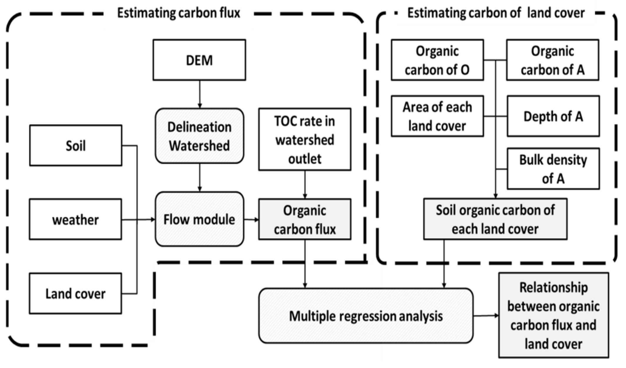
This study was conducted in three steps.
In the first step, applicable sample watersheds were delineated and the carbon flux for each watershed was estimated. In the second step, the land cover area for each watershed was calculated and the SOC for each land cover type was estimated. In the third step, the relationship between the land cover area and SOC in the watershed, and the amount of carbon flux, were analyzed (Figure 1).
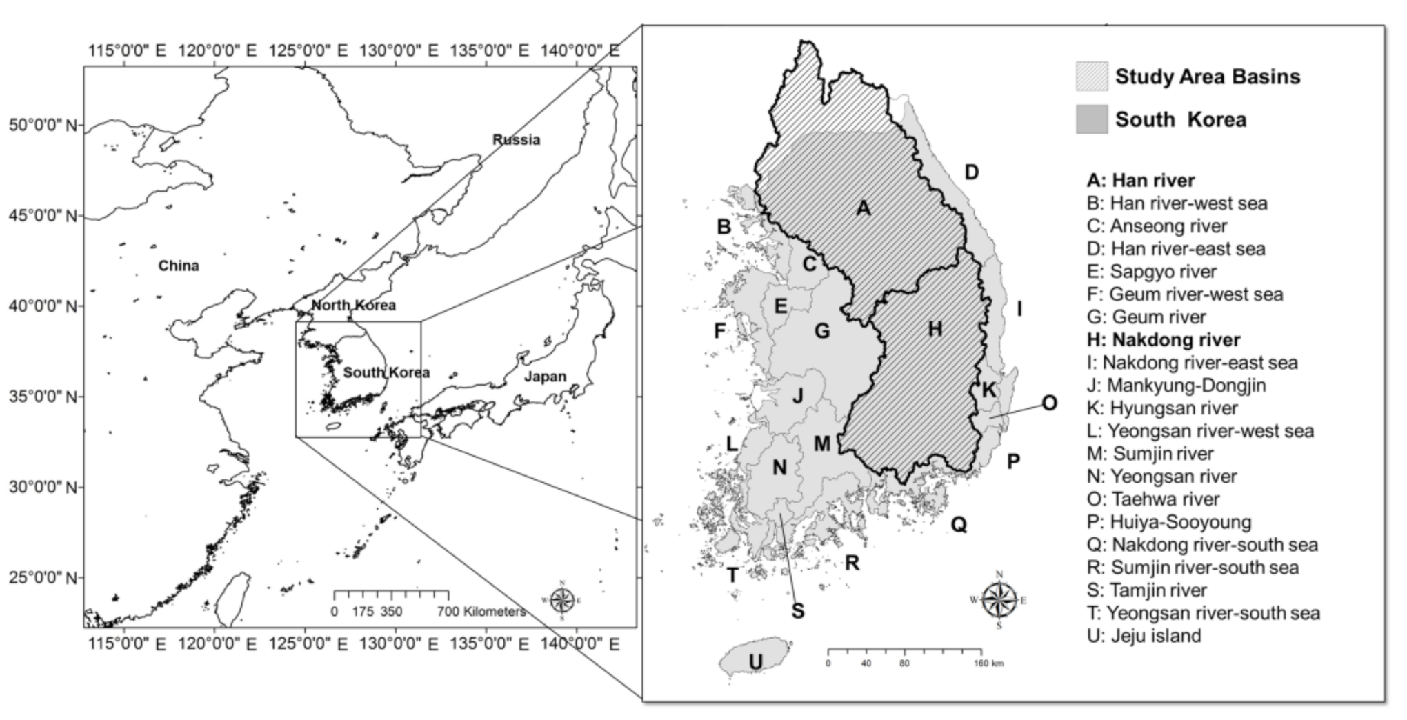
2.1. Study Area and Watershed Samples
To conduct this research, a study site was selected in South Korea. Because South Korea has accumulated land cover, soil, forest, and river data for the entire country, it is easy to study carbon flux on a national scale. To understand the carbon cycle processes from forest to river in South Korea, a study was previously conducted in Gwangneung broadleaved forests, where it estimated the carbon runoff rate of soil organic carbon according to specific trees [14].
The study areas were the Han and Nakdong River basins, the two largest basins in South Korea (Figure 2), with a combined area of 49,337.8 km2, which covers more than half of the total area of South Korea (100,339.5 km2). The total river length involved was 14,417 km, representing approximately 48% of the 29,817 km total river length of South Korea. The flow rate of the two basins is 44 G m3 year−1, which accounted for 58.4% of the total flow rate of 75.3 G m3 year−1 in South Korea. The average annual precipitation in South Korea is 1306.3 mm, and the summer precipitation is 710.9 mm, accounting for 54% of the annual precipitation. By month, the average monthly temperature is 19.7~26.7 °C in August, the hottest month, and −6.9~3 °C in January, the coldest month [15]. As this accounts for more than half of South Korea’s hydrological quantitative factors, the results from these two basins can be considered to represent the overall hydrological trends for South Korea.
The carbon flux from land to rivers could be estimated on a watershed basis. The watersheds were classified by shape type into those with only river outlets and others with both inlets and outlets. It was difficult to analyze the effect of land cover alone in a watershed with inlets because the amount of carbon flux from the inlets must also be taken into account. Therefore, in this study, only watersheds with outlets were considered.
The ability to discharge SOC is a natural environmental factor; therefore, urban land cover was not covered in this study. Moreover, impervious areas cannot release SOC directly, and some studies have noted that if the percentage of impervious areas is more than 10%, it could affect water quality [16,17,18]. In this study, we analyzed the natural ability to discharge SOC based on forest and agricultural land cover in watersheds with an urban area of less than 10%. If the urban area of a potential study site exceeded 10%, the site was excluded from this analysis; after which, a total of 82 watershed samples remained (Table 1). The total area of the watershed sampling sites was 10,773 km2, which was approximately 11% of the total area of South Korea. The smallest sampling area was 12.41 km2 and the largest was 829.18 km2.
2.2. Estimating Carbon Flux of Each Watershed Sample
The carbon flux for each watershed was estimated, using Equation (1). In Equation (1), carbon flux is the amount of carbon released from the watershed in tons/year, flow rate is the amount of water released from the watershed in m3/year, and TOC concentration is the total organic carbon concentration at each watershed outlet in mg/L.
Carbon Flux = Flow Rate × TOC concentration
In South Korea, the Ministry of Land, Infrastructure, and Transport (MoLIT) measures river flow rates, whereas the Ministry of Environment (MoE) measures organic carbon concentration. Each institution has its own monitoring location. Therefore, spatial data compatibility was a challenge in this study.
Because the location of TOC measurement points and flow measurement points were different, it was effective to delineate basins based on one kind of measurement point and to estimate other values of the point using a hydrological model. In the literature on the calibration of hydrological models, flow rate verification is performed first because the factor used to estimate the flow rate also affects the water-quality estimate [19]. In other words, water-quality estimation required more data than did flow-rate estimation, and the water-quality-estimation value could contain more uncertainty than the estimated flow rate value. Therefore, in this study, the watershed samples with water-quality measurement points as outlets were delineated and the flow rates were estimated based on the water-quality measurement points. To estimate the flow rates at these points, the Soil and Water Assessment Tool (SWAT), which is a hydrological modeling tool based on physical parameters, was used. By using the delineating watershed function of Arc-SWAT and a digital elevation model (DEM), watersheds could be delineated, based on the water-quality measurement points.
The SWAT model is a physical hydrological model developed by the US Department of Agriculture (USDA), which is built on predecessor models such as CLEAMS, EPIC, and CREAMS, developed by USDA-ARS (Agricultural Research Service), and has the particular strength of being a long-term simulation tool [20]. There have been many research studies in which the SWAT model was applied, and it has been widely used worldwide. Inputs needed for the SWAT model are meteorological data, such as daily precipitation, maximum/minimum temperature, solar radiation, relative humidity and wind speed, and geographical data, such as land cover, soil mapping, and digitized elevations, derived from a DEM.
The DEM used in this study was the Advanced Spaceborne Thermal Emission and Reflection Radiometer Global DEM provided by the United States National Aeronautics and Space Administration (NASA) and its spatial resolution is 30 m. The simulation results could vary according to spatial resolution. In a previous study, it was stated that a DEM with a resolution of 30 m could be used in the hydrological study [21].
The land cover map was obtained from the MoE, the soil map was obtained from the South Korea Rural Development Administration (RDA), and meteorological data were obtained from the Korea Meteorological Administration (KMA).
The flow rate estimated by the SWAT model was calibrated and validated with flow data from the MoLIT. The SWAT-CUP program was developed for the calibrating SWAT model [22,23]. The SWAT-CUP is a program that tests for optimal parameters by setting and running the parameters according to the algorithm within ranges set by the researcher. In this study, model calibration and validation were performed for the Nakdong River and Han River basins, and monthly average flow rates were used. The model calibration process was continued until the percentage difference between measured and estimated average monthly values was less than 15%, the coefficient of determination was greater than 0.6, and the Nash-Sutcliffe efficiency coefficient (a coefficient widely used to calibrate hydrological models) was greater than 0.5 [19,24].
The results of this study may be influenced by weather extremes. To alleviate this, simulation periods should be long-term, more than 30 years. However, owing to carbon concentration data only being available since 2012, the research period commenced in 2012. The simulation period overall was from 2010 to 2016, and the model commencement period was from 2010 to 2011.
2.3. Estimating Soil Organic Carbon of Each Land Cover Type
Land cover is the observed physical cover on the earth’s surface, classified by use and other characteristics, giving each land cover type specific properties [25]. Each watershed sample was classified as forest, agricultural land, and urban land using the cover map of the MoE. The types “barren”, “grasslands”, and “wetlands” were excluded from this study because the percentage of these land covers was very low, suggesting that these land cover types would not be impressive to sample watersheds.
Forest SOC was estimated using the Forest Biomass and Dead Organic Matter Carbon model (FBDC). The FBDC is a process-based model for estimating forest carbon cycles by calculating dynamics between forest carbon pools, primary dead organic matters, and secondary dead organic matters [26]. The FBDC is effective in studying forests in South Korea and has been used in several previous studies [27,28,29].
The SOC for agricultural land was estimated in different ways for each layer. The amount for the A layer was estimated using soil data from the RDA. The land cover and soil maps were overlaid to extract only the soils of the agricultural land. Then, the SOC value down to 1 m in depth for agricultural land cover was estimated by using Equation (2). In Equation (2), SOC is the SOC for the A layer in k ton; area is measured in km2; depth is measured in mm; bulk density is measured in g mL−1, and OC is organic carbon, in percent.
SOC = Area × Depth × Bulk Density × OC
To obtain estimated values for the O layer, the designation “dead organic matter and live biomass consumption value for fire in a range of vegetation types”, from the IPCC Guidelines for National Greenhouse Gas Inventories tier 1 method was adopted [30]. Because rice fields are the major agricultural land use in South Korea, the value for “rice residue” was used [31].
2.4. Regression Analysis
To elucidate the relationship between land cover and the carbon flux from watershed to rivers, regression analyses were performed. In this study, regression analyses were conducted in two aspects. To begin, we wanted to create an equation that could be used to arithmetically estimate the carbon flux in watershed area.
The second regression analysis was performed between the land cover type SOC and the carbon flux, both divided by the watershed area. Through this analysis, the influence and trend of each land cover type on the carbon flux could be better understood.
3. Results
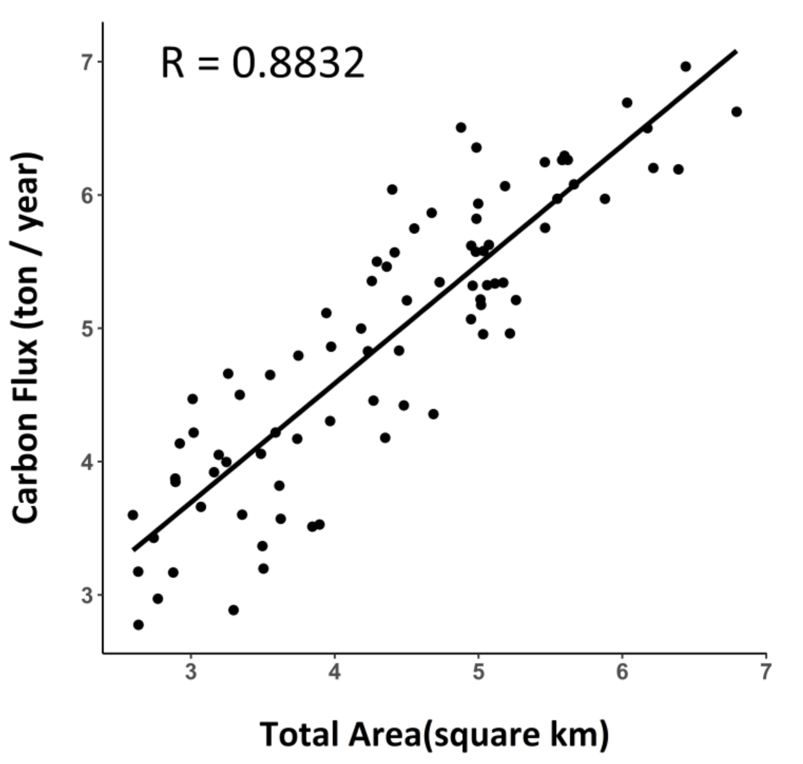
3.1. Relationship between Watershed Area and Carbon Flux
The flow rate of the rivers was derived from the watershed; therefore, it was clear that the larger the watershed area, the larger the carbon flux of the watershed. Pearson correlation analysis was performed between the watershed area and the carbon flux of 82 watershed samples, and it was confirmed that there was a high positive correlation between the two comparative factors (Figure 3). The Pearson correlation coefficient was 0.8832.
It was statistically confirmed that the carbon flux increased as the watershed area increased. Additionally, the carbon flux tended to increase as the SOC increased because the larger the area of the watershed, the greater the amounts of SOC stored in the watershed, and the greater the amount of runoff from the watershed. An empirical model Equation (3) shows the proportional relationship between the watershed area and the carbon flux (Table A1). The coefficient of determination in Equation (3) is 0.7774, and it is considered that Equation (3) has considerable explanatory power. In Equation (3), carbon flux is in ton year−1; watershed area is in km2.
ln (Carbon Flux) = 1.01654 + 0.89271 × ln (Watershed area)
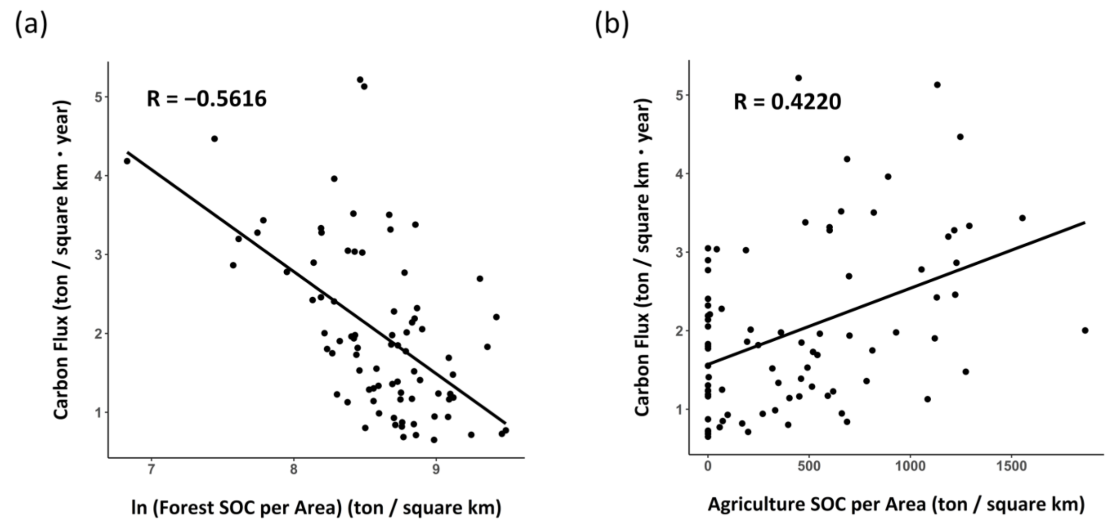
3.2. Relationship between Soil Organic Carbon per Watershed Area of Each Land Cover and Carbon Flux per Watershed Area
Regression analysis was performed between the SOC for each land cover divided by the total watershed area, as well as the amount of carbon flux divided by watershed area. The purpose of this analysis was to investigate the effect of land cover on SOC runoff from land in the same watershed area.
The correlation coefficient between the carbon flux per watershed area and forest SOC per watershed area converted to log form was −0.5616 (Figure 4). As forest SOC increases, carbon flux is thought to decrease nonlinearly. The correlation coefficient between the carbon flux per watershed area and agricultural land SOC per watershed area was 0.422 (Figure 4). In the results of the multiple regression analysis, the coefficient of determination of the whole regression equation was 0.264 (Table 2). The regression coefficient for agricultural land SOC did not meet the significance level of 0.05.
Agricultural land cover seemed to have little or irregular influence on the mechanism of soil carbon runoff; however, forest cover showed a tendency towards decreasing carbon flux as the SOC increased. Considering estimates derived from the two models were used in the analysis and the distribution of scattering could be visualized as a logarithmic decrease, −0.5616, the correlation coefficient, may be reasonable. This result showed that forests can make carbon flux decrease.
3.3. Carbon Flux per Watershed Area in Forest Land Cover
Above ground biomass in forests is an indicator of how well-developed forests are. In addition, one of the largest sources of forest SOC is the above ground part of the forest. Thus, the higher the amount of carbon above ground, the greater the amount of carbon stored in the forest soil, and the lower the carbon flux of the watershed.
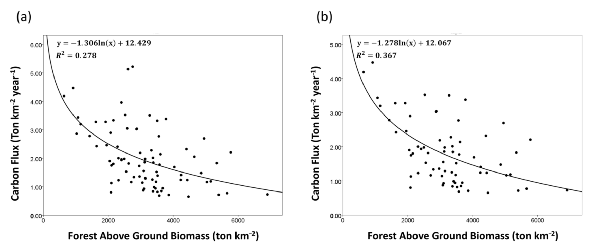
In the previous analysis, it was confirmed that the forest land cover affects the carbon flux, and further analysis was performed on the forest. Regression analysis was performed between the forest above ground biomass, estimated using the FBDC model, and carbon flux. The result showed that the carbon flux decreased logarithmically as the forest above ground biomass increased. The coefficient of determination was 0.278, which was lower than that of the previous analysis using forest SOC. However, considering that the soil and below ground biomass were locations from which the actual organic carbon was released, and that the above ground forest carbon affects soil carbon, the 0.278 coefficient of determination was considered to be reasonable.
In addition, some annual precipitation in data was relatively extreme because the microclimates of each watershed differed. To reduce the influence of precipitation, we conducted further analysis using only data from watersheds with average precipitation from 950 mm to 1300 mm. In this analysis, the coefficient of determination increased to 0.367. Therefore, the forest land cover affects carbon flux depending on the forest above ground biomass, and carbon flux may also vary with precipitation (Figure 5).
Multiple regression analysis was performed using the natural logarithm of forest above ground biomass and the annual precipitation of the watershed. The adjusted coefficient of determination was 0.351, and this indicated that the influence of forest above ground biomass and precipitation accounted for 35% of the annual carbon flux (Table A2).
The results showed that the more SOC and above ground biomass were held by the forests, the more the carbon flux tended to decrease. As the forest above ground biomass increased, carbon flux decreased logarithmically. Annual precipitation factors affecting carbon flux were also considered, and a statistical model equation was derived (Equation (4)). In Equation (4), carbon flux is in ton y−1 km−2, p is annual precipitation of the watershed, in mm; and AGB is forest above ground biomass, in ton km−2.
Carbon Flux = 9.252 + 0.002 × p + (−1.265) × ln (AGB)
4. Discussion
4.1. Carbon Flux and Watershed Area
Statistics can help in understanding the phenomena and provide numerical guidelines when planning. In this study, it was found that the carbon flux and the watershed area were proportional to each other, and Equation (3) is an empirical model that combined the results based on this knowledge. In general, hydrologic models require a lot of data and preparation. Therefore, Equation (3) may be useful when conducting pilot studies, before starting the study of carbon fluxes in watersheds. It was confirmed through several cases that certain estimated values can be helpful for follow-up research on the specific study area, and Equation (3) can be applied when studying a specific watershed in South Korea [14,32]. The same equation can be used to study watersheds in other study area with similar climates. In other countries and climates, the same method can be used to derive the equation.
4.2. Carbon Flux and Forest Carbon Pool
In this study, we found that the more AGBs in forests located in the watershed, the lower the carbon flux in the watershed. In addition, there was no significant effect of agricultural land on carbon flux. The causes of the results in this study have been shown in previous studies. SOC on land is released as particulate organic carbon (POC) and dissolved organic carbon (DOC). POC is carbon in the form of water-insoluble particles, usually released from weathered soil [4]. DOC is a type of carbon that is dissolved in water and its discharge pattern can be influenced by precipitation, catchment characteristics, and soil type [5].
For POC, soil loss occurs more from barren cover than from forest cover areas, because thick forest litter catches the soil, thereby preventing erosion and reducing soil loss [32,33]. In addition, roots or thick litter layers of fallen leaves catch the soil, and also absorb water, reducing runoff in forests.
For DOC, a past study showed that approximately 74% of DOC concentration was accounted for through weather and topographical factors [34]. Because forest development has less influence on the DOC concentration and the amount of outflow water is decreased in well-developed forests, it follows that the amount of DOC released is decreased as the forest develops.
Previous studies that have analyzed forest cover have done so by studying plant species that occupy the forest. In this study, we performed an analysis based on the degree of forest development using the forest model. In well-developed forests, carbon stored in the soil is increased, but carbon flux through precipitation was lower than that in less-developed forests. In other words, the SOC of forests can be regarded as an indicator of carbon release capacity, not just a carbon pool in the carbon flux mechanism.
Finally, in agricultural land, if the soil loss and the lateral runoff of rainwater are the same, the larger the SOC stored, the more carbon was released. Therefore, it seems that the negative effect seen in the forest land cover is special, and the positive effect seen in the agriculture land cover seems reasonable. Rather, the pattern of carbon flux increase according to the SOC of agricultural land is not constant, which seems to be due to the influence of organic matter by human activities other than SOC or the error in the carbon estimation of the agricultural land O layer used in this study.
4.3. Carbon Management and Forests
Since the Paris Agreement, the LULUCF (Land Use, Land-Use Change and Forestry) sector is essential for achieving Nationally Determined Contributions (NDC), which should be developed by countries [35,36]. LULUCF means the increase or decrease of the greenhouse gas that changes according to land use. IPCC Guidelines have been produced, and information by land use type is the basis for carbon stock change and estimation of greenhouse gas emissions and removals [30]. Therefore, a study approaching the carbon cycle from the land cover point of view should be conducted. In South Korea, some studies have been carried out to build a forest LULUCF greenhouse gas inventory [37].
Carbon flux mediated through precipitation, which affects the hydrological runoff associated with DOC and soil erosion associated with POC, and respiration of vegetation and soil are the main mechanisms for carbon emissions from land [3]. Forests can store carbon in vegetation and soil, and as a forest are more developed, it can store more carbon. Moreover, this study found that well-developed forests release less organic carbon through precipitation. This means that a well-developed forest can play a role as carbon reserves. In addition, this study confirmed that the amount of carbon flux from watershed can be quantified using the amount of carbon held by forests. These findings can be used to make effective management plans to achieve LULUCF and NDC goals.
4.4. Limitations
Three key limitations of this study have remained.
First, this study excluded human influence. Because the objective of this study was to estimate the soil carbon runoff coefficient, human influence was excluded to the maximum extent possible, and only watershed samples with less than 10% urban area were studied. Subsequently, quantifying human effects will help estimate the carbon flux accurately. Furthermore, in terms of the environment, human activities such as forest management and increasing atmospheric nitrogen input, which can affect the translocation and transformation of soil organic carbon in the soil–river systems, should be considered.
Second, in forests in their early stages, carbon flux can increase as SOC increases, because early forests are likely to lack the ability to reduce carbon discharge. However, because the barren area in the study area was very small, extracting watershed samples from barren land was impossible.
Third, Equation (4) had low explanatory power. The coefficient of determination of 0.35 was considered to be a reasonable value because the two estimated model values were used, and the logarithmical declining form was revealed. However, the result implies that forest cover and precipitation combined accounted for only 35% of the carbon flux. To explain the remaining balance, natural factors, such as temperature and slope, and artificial factors such as human activity, would need to be included in the analysis. In particular, it is anticipated that the organic carbon content of pollutants coming from human activities could be large because organic materials can be discharged from domestic sewage or agricultural sewage. Therefore, it is expected that the inclusion of human influences is necessary for future research, to determine the influence of urban and agricultural cover on the total carbon flux.
5. Conclusions
In this study, it was found that forest land cover type affected carbon runoff from watershed to rivers, and the relationship was described by regression model equations. The carbon flux from the watershed was estimated using the SWAT model, incorporating water quality data from the MoE. Then, the amount of SOC in the forest was estimated using the FBDC model, and the amount of SOC in agricultural land was estimated using the IPCC carbon inventory methodology with RDA data. Lastly, statistical analyses were performed by integrating the area for each watershed sample, the SOC from each land cover, and the carbon flux of the watershed.
The findings from this study were as follows: (1) As the area of the basin increased, the carbon flux increased. (2) As forests developed and AGB increased, the carbon runoff decreased logarithmically. This was believed to be due to the specific characteristics of forest cover. (3) This study showed that forest land cover had a changeable carbon release capacity, as represented by Equation (4). (4) From the perspective of looking at forests as carbon reservoirs, it was considered to be a key finding that well-developed forests were outstanding carbon storage reservoirs.
The results of this study could be useful for studying land and river ecosystems, and for national carbon management, especially when targeting temperate forests with a temperate climate. To accurately grasp the carbon flux mechanism of the watershed, research should be conducted taking into consideration urban effects and the early stage of forests.
Author Contributions
Conceptualization, G.-S.K. and S.-g.L.; Methodology, G.-S.K., S.-g.L., J.L. and C.S.; Validation, G.-S.K.; Formal Analysis, G.-S.K.; Investigation, S.-g.L., E.P., M.H. and Y.-J.K.; Resources, G.-S.K., S.-g.L. and J.L.; Data Curation, G.-S.K., S.-g.L. and J.L.; Writing-Original Draft Preparation, G.-S.K. and E.P.; Writing-Review and Editing, G.-S.K., S.-g.L. and J.L.; Visualization, G.-S.K.; Supervision, W.-K.L.; Project Administration, W.-K.L.; Funding Acquisition, W.-K.L. All authors have read and agreed to the published version of the manuscript.
Funding
This research was supported by Basic Science Research Program through the National Research Foundation of Korea (NRF) funded by the Ministry of Education (NRF-2021R1A6A1A10045235) and also supported under the NRF’s framework of an international cooperation program (2021K2A9A1A02101519).
Institutional Review Board Statement
Not applicable.
Informed Consent Statement
Not applicable.
Data Availability Statement
Not applicable.
Acknowledgments
This paper is an excerpt from the Master Thesis with the title “Estimating the carbon runoff coefficient from land to river by land cover type in South Korea.” written by Gang Sun Kim as part of his studies at the Department of Environmental Science and Ecological Engineering graduate school of the Korea University (Korea) in August 2018.
Conflicts of Interest
The authors declare no conflict of interest.
Appendix A

Table A1.
Results of regression analysis between watershed area and carbon flux (both variables are converted to natural log form).
Table A1.
Results of regression analysis between watershed area and carbon flux (both variables are converted to natural log form).
| Revised Coefficient of Determination | Degree of Freedom | F | p-Value | |||
|---|---|---|---|---|---|---|
| 0.7774 | 81 | 283.9 | 2.2 × 10⁻¹⁶ | |||
| Variables | Estimate | Std. Error | t-Value | p-Value | VIF | |
| Intercept | 1.01654 | 0.23806 | 4.27 | 5.33 × 10⁻⁵ | - | |
| Watershed area | 0.89271 | 0.05299 | 16.85 | 2 × 10⁻¹⁶ | - | |
Table A2.
Results of multiple regression analysis between the forest above ground biomass and precipitation and carbon flux.
Table A2.
Results of multiple regression analysis between the forest above ground biomass and precipitation and carbon flux.
| Revised Coefficient of Determination | Degree of Freedom | F | p-Value | |||||
|---|---|---|---|---|---|---|---|---|
| 0.351 | 81 | 22.875 | 1.45 × 10⁻⁸ | |||||
| Variables | Estimate | Std. Error | t-Value | p-Value | VIF | |||
| Intercept | 9.252 | 2.012 | 4.598 | 1.61 × 10⁻⁵ | - | |||
| Precipitation | 0.002 | 0.001 | 3.321 | 0.001 | 1.003 | |||
| Natural logarithm of forest above ground biomass | −1.265 | 0.222 | −5.6999 | 1.9956 × 10⁻⁷ | 1.003 | |||
References
- Heimann, M.; Reichstein, M. Terrestrial ecosystem carbon dynamics and climate feedbacks. Nature 2008, 451, 289–292. [Google Scholar] [CrossRef] [PubMed]
- Smith, R.L. Elements of Ecology; Harper & Row: New York, NY, USA, 1986. [Google Scholar]
- Ciais, P.; Sabine, C.; Bala, G.; Bopp, L.; Brovkin, V.; Canadell, J.; Chhabra, A.; DeFries, R.; Galloway, J.; Heimann, M.; et al. Carbon and other biogeochemical cycles. In Climate Change 2013: The Physical Science Basis; Cambridge University Press: Cambridge, UK, 2013; pp. 465–570. [Google Scholar]
- Meybeck, M.; Vörösmarty, C. Global transfer of carbon by rivers. Glob. Change Newsl. 1999, 37, 18–19. [Google Scholar]
- Strohmeier, S.; Knorr, K.-H.; Reichert, M.; Frei, S.; Fleckenstein, J.H.; Peiffer, S.; Matzner, E. Concentrations and fluxes of dissolved organic carbon in runoff from a forested catchment: Insights from high frequency measurements. Biogeosciences 2013, 10, 905–916. [Google Scholar] [CrossRef] [Green Version]
- Comber, A.; Fisher, P.; Wadsworth, R. What is land cover? Environ. Plan. B Plan. Design 2005, 32, 199–209. [Google Scholar] [CrossRef] [Green Version]
- Townshed, J.; Justice, C.; Li, W.; Gurney, C.; McManus, J. Global land cover classification by remote sensing: Present capa-bilities and future possibilities. Remote Sens. Environ. 1991, 35, 243–255. [Google Scholar] [CrossRef]
- Sobrino, J.A.; Raissouni, N. Toward remote sensing methods for land cover dynamic monitoring: Application to Morocco. Int. J. Remote Sens. 2000, 21, 353–366. [Google Scholar] [CrossRef]
- Jacinthe, P.-A.; Lal, R.; Owens, L.; Hothem, D. Transport of labile carbon in runoff as affected by land use and rainfall characteristics. Soil Tillage Res. 2004, 77, 111–123. [Google Scholar] [CrossRef]
- Veum, K.S.; Goyne, K.W.; Motavalli, P.P.; Udawatta, R.P. Runoff and dissolved organic carbon loss from a paired-watershed study of three adjacent agricultural Watersheds. Agric. Ecosyst. Environ. 2009, 130, 115–122. [Google Scholar] [CrossRef]
- Beguería, S.; Angulo-Martinez, M.; Gaspar, L.; Navas, A. Detachment of soil organic carbon by rainfall splash: Experimental assessment on three agricultural soils of Spain. Geoderma 2015, 245-246, 21–30. [Google Scholar] [CrossRef] [Green Version]
- Bachman, M.; Inamdar, S.; Barton, S.; Duke, J.M.; Tallamy, D.; Bruck, J. A Comparative assessment of runoff nitrogen from turf, forest, meadow, and mixed landuse watersheds. JAWRA J. Am. Water Resour. Assoc. 2016, 52, 397–408. [Google Scholar] [CrossRef]
- Turner, J.; Lambert, M. Pattern of carbon and nutrient cycling in a small Eucalyptus forest catchment, NSW. For. Ecol. Manag. 2016, 372, 258–268. [Google Scholar] [CrossRef]
- Kim, S.J.; Kim, J.; Kim, K. Organic carbon efflux from a deciduous forest catchment in Korea. Biogeosciences 2010, 7, 1323–1334. [Google Scholar] [CrossRef] [Green Version]
- Korea Meteorological Agency. Korea Climate Characteristic. Available online: https://www.weather.go.kr/w/obs-climate/climate/korea-climate/korea-char.do (accessed on 27 January 2022).
- Arnold, C.L., Jr.; Gibbons, C.J. Impervious surface coverage: The emergence of a key environmental indicator. J. Am. Plan. Assoc. 1996, 62, 243–258. [Google Scholar] [CrossRef]
- Schueler, T. The importance of imperviousness. Watershed Prot. Tech. 1994, 1, 100–101. [Google Scholar]
- Liu, Z.; Wang, Y.; Li, Z.; Peng, J. Impervious surface impact on water quality in the process of rapid urbanization in Shenzhen, China. Environ. Earth Sci. 2012, 68, 2365–2373. [Google Scholar] [CrossRef]
- Santhi, C.; Arnold, J.G.; Williams, J.R.; Dugas, W.A.; Srinivasan, R.; Hauck, L.M. Validation of the SWAT model on a large river basin with point and nonpoint sources. JAWRA J. Am. Water Resour. Assoc. 2001, 37, 1169–1188. [Google Scholar] [CrossRef]
- Gassman, P.W.; Reyes, M.R.; Green, C.H.; Arnold, J.G. The soil and water assessment tool: Historical development, appli-cations, and future research directions. Trans. Am. Soc. Agr. Biol. Eng. 2007, 50, 1211–1250. [Google Scholar]
- Korea Institute of Construction Technology. A Study on the Improvement of the Supporting System of Water Resources in National GIS Project; Korea Institute of Construction Technology: Goyang-si, Korea, 2002. [Google Scholar]
- Abbaspour, K.C.; Yang, J.; Maximov, I.; Siber, R.; Bogner, K.; Mieleitner, J.; Zobrist, J.; Srinivasan, R. Modelling hydrology and water quality in the pre-alpine/alpine Thur watershed using SWAT. J. Hydrol. 2007, 333, 413–430. [Google Scholar] [CrossRef]
- Abbaspour, K.C. SWAT Calibration and Uncertainty Programs—A User Manual; Swiss Federal Institute of Aquatic Science and Technology: Eawag, Switzerland, 2015. [Google Scholar]
- Nash, J.E.; Sutcliffe, J.V. River flow forecasting through conceptual models part I—A discussion of principles. J. Hydrol. 1970, 10, 282–290. [Google Scholar] [CrossRef]
- Di Gregorio, A. Land Cover Classification System: Classification Concepts and User Manual: LCCS (No. 8); Food and Agriculture Organization of the United Nations (FAO): Rome, Italy, 2005. [Google Scholar]
- Lee, J.; Yoon, T.K.; Han, S.; Kim, S.; Yi, M.J.; Park, G.S.; Kim, C.; Son, Y.M.; Kim, R. Estimating the carbon dynamics of South Korean forests from 1954 to 2012. Biogeosciences 2014, 11, 4637–4650. [Google Scholar] [CrossRef] [Green Version]
- Lee, J.; Tolunay, D.; Makineci, E.; Çömez, A.; Son, Y.M.; Kim, R.; Son, Y. Estimating the age-dependent changes in carbon stocks of Scots pine (Pinus sylvestris L.) stands in Turkey. Ann. For. Sci. 2016, 73, 523–531. [Google Scholar] [CrossRef] [Green Version]
- Lee, J.; Lee, S.; Han, S.H.; Kim, S.; Roh, Y.; Abu Salim, K.; Pietsch, S.A.; Son, Y. Estimating carbon dynamics in an intact lowland mixed dipterocarp forest using a forest carbon model. Forests 2017, 8, 114. [Google Scholar] [CrossRef] [Green Version]
- Lee, J.; Lim, C.H.; Kim, G.S.; Markandya, A.; Chowdhury, S.; Kim, S.J.; Lee, W.K.; Son, Y. Economic viability of the na-tional-scale forestation program: The case of success in the Republic of Korea. Ecosyst. Serv. 2018, 29, 40–46. [Google Scholar] [CrossRef]
- Aalde, H.; Gonzalez, P. Generic Methodologies Applicable to Multiple Land-Use Categories. In 2006 IPCC Guidelines for National Greenhouse Gas Inventories; IPCC: Geneva, Switzerland, 2006. [Google Scholar]
- FAO. AQUASTAT Country Profile–Democratic People’s Republic of Korea; Food and Agriculture Organization of the United Nations (FAO): Rome, Italy, 2011. [Google Scholar]
- Kim, G.S.; Lim, C.-H.; Kim, S.J.; Lee, J.; Son, Y.; Lee, W.-K. Effect of national-scale afforestation on forest water supply and soil loss in South Korea, 1971–2010. Sustainability 2017, 9, 1017. [Google Scholar] [CrossRef] [Green Version]
- Blanco-Canqui, H.; Lal, R. Soil erosion under forest. In Principles of Soil Conservation and Management; Springer: Berlin/Heidelberg, Germany, 2010; pp. 321–344. [Google Scholar]
- Jutras, M.-F.; Nasr, M.; Castonguay, M.; Pit, C.; Pomeroy, J.H.; Smith, T.P.; Zhang, C.-F.; Ritchie, C.D.; Meng, F.-R.; Clair, T.A.; et al. Dissolved organic carbon concentrations and fluxes in forest catchments and streams: DOC-3 model. Ecol. Model. 2011, 222, 2291–2313. [Google Scholar] [CrossRef]
- Pistorius, T.; Reinecke, S.; Carrapatoso, A. A historical institutionalist view on merging LULUCF and REDD+ in a post-2020 climate agreement. Int. Environ. Agreem. Politics Law Econ. 2016, 17, 623–638. [Google Scholar] [CrossRef]
- Fyson, C.; Jeffery, L. Examining treatment of the LULUCF sector in the NDCs. In EGU General Assembly Conference Abstracts; EGU2018: Vienna, Austria, 2018; Volume 20, p. 16542. [Google Scholar]
- Park, E.; Song, C.; Ham, B.; Kim, J.; Lee, J.; Choi, S.-E.; Lee, W.-K. Comparison of Sampling and Wall-to-Wall Methodologies for Reporting the GHC Inventory of the LULUCF Sector in Korea. J. Clim. Change Res. 2018, 9, 385–398. [Google Scholar] [CrossRef]
Figure 1.
Research process of this study.

Figure 2.
Study area (Han River basin and Nakdong River basin).

Figure 3.
Relationship between total area of watershed and carbon flux (both variables are converted to natural log form).
Figure 3.
Relationship between total area of watershed and carbon flux (both variables are converted to natural log form).

Figure 4.
(a) Relationship between forest soil organic carbon per watershed area (converted to natural log form) and carbon flux per watershed area, (b) relationship between agricultural land soil organic carbon per watershed area and carbon flux per watershed area.
Figure 4.
(a) Relationship between forest soil organic carbon per watershed area (converted to natural log form) and carbon flux per watershed area, (b) relationship between agricultural land soil organic carbon per watershed area and carbon flux per watershed area.

Figure 5.
(a) Relationship between forest above ground biomass and carbon flux, (b) relationship between forest above ground biomass and carbon flux, except outliers (except carbon flux at precipitation extremes).
Figure 5.
(a) Relationship between forest above ground biomass and carbon flux, (b) relationship between forest above ground biomass and carbon flux, except outliers (except carbon flux at precipitation extremes).

Table 1.
Information on watershed samples from the Han River basin and Nakdong River basin.
| Basin | The Number of Samples | Watershed Samples Area (km2) | Forest Area (km2) | Agricultural Land Area (km2) | River Length Extension (km) |
|---|---|---|---|---|---|
| Han River | 42 | 4234.436 | 3351.157 | 875.595 | 1163.646 |
| Nakdong River | 40 | 6538.066 | 5526.772 | 1394.709 | 1788.121 |
| Total | 82 | 10,772.5 | 8477.93 | 2270.304 | 2951.767 |
Table 2.
Results of multiple regression analysis between soil organic carbon of each land cover type per watershed area and carbon flux.
Table 2.
Results of multiple regression analysis between soil organic carbon of each land cover type per watershed area and carbon flux.
| Revised Coefficient of Determination | Degree of Freedom | F | p-Value | ||
|---|---|---|---|---|---|
| 0.264 | 81 | 15.503 | 2 × 10⁻⁶ | ||
| Variables | Estimate | Std. Error | t-Value | p-Value | VIF |
| Intercept | 2.734 | 0.37216 | 7.347 | 1.61 × 10⁻¹⁰ | - |
| Natural logarithm of Forest SOC per Watershed Area | 1.61 × 10⁻⁴ | 4.8 × 10⁻⁵ | −3.378 | 0.0011 | 1.375 |
| Agricultural Land SOC per Watershed Area | 5.16 × 10⁻⁴ | 2.57 × 10⁻⁴ | 2.012 | 0.48 | 1.375 |
Publisher’s Note: MDPI stays neutral with regard to jurisdictional claims in published maps and institutional affiliations. |
© 2022 by the authors. Licensee MDPI, Basel, Switzerland. This article is an open access article distributed under the terms and conditions of the Creative Commons Attribution (CC BY) license (https://creativecommons.org/licenses/by/4.0/).
Share and Cite
MDPI and ACS Style
Kim, G.-S.; Lee, S.-g.; Lee, J.; Park, E.; Song, C.; Hong, M.; Ko, Y.-J.; Lee, W.-K. Effects of Forest and Agriculture Land Covers on Organic Carbon Flux Mediated through Precipitation. Water 2022, 14, 623. https://doi.org/10.3390/w14040623
AMA Style
Kim G-S, Lee S-g, Lee J, Park E, Song C, Hong M, Ko Y-J, Lee W-K. Effects of Forest and Agriculture Land Covers on Organic Carbon Flux Mediated through Precipitation. Water. 2022; 14(4):623. https://doi.org/10.3390/w14040623
Chicago/Turabian StyleKim, Gang-Sun, Sle-gee Lee, Jongyeol Lee, Eunbeen Park, Cholho Song, Mina Hong, Young-Jin Ko, and Woo-Kyun Lee. 2022. "Effects of Forest and Agriculture Land Covers on Organic Carbon Flux Mediated through Precipitation" Water 14, no. 4: 623. https://doi.org/10.3390/w14040623
Note that from the first issue of 2016, this journal uses article numbers instead of page numbers. See further details here.