
Evaluating Multiple Stressor Effects on Benthic–Pelagic Freshwater Communities in Systems of Different Complexities: Challenges in Upscaling

 ,
,  , , , , , ,
  , , , and
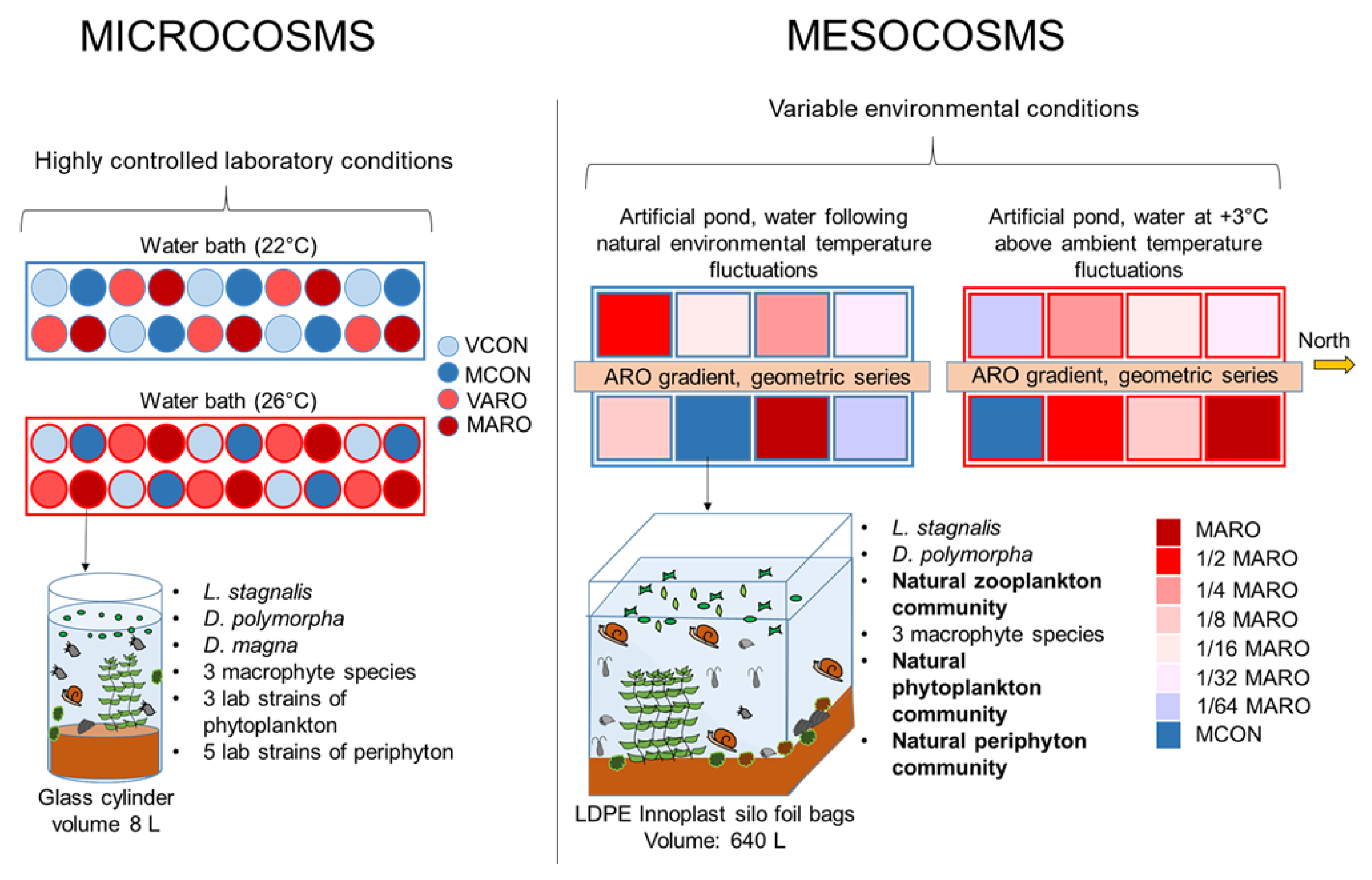
Abstract
:1. Introduction
- Water type will not modify effects of the stressors;
- Response of model (laboratory) communities to the stressors can be mirrored in more complex field (mesocosm) communities;
- A gradient design will allow for the detection of concentration-dependent community effects in more complex systems.
2. Materials and Methods
2.1. Microcosm Experiment
2.1.1. Set-Up and Design
2.1.2. Sampling and Measured Parameters
2.1.3. Data Analysis
2.2. Mesocosms
2.2.1. Set-Up and Design
2.2.2. Sampling and Measured Parameters
2.2.3. Data Analysis
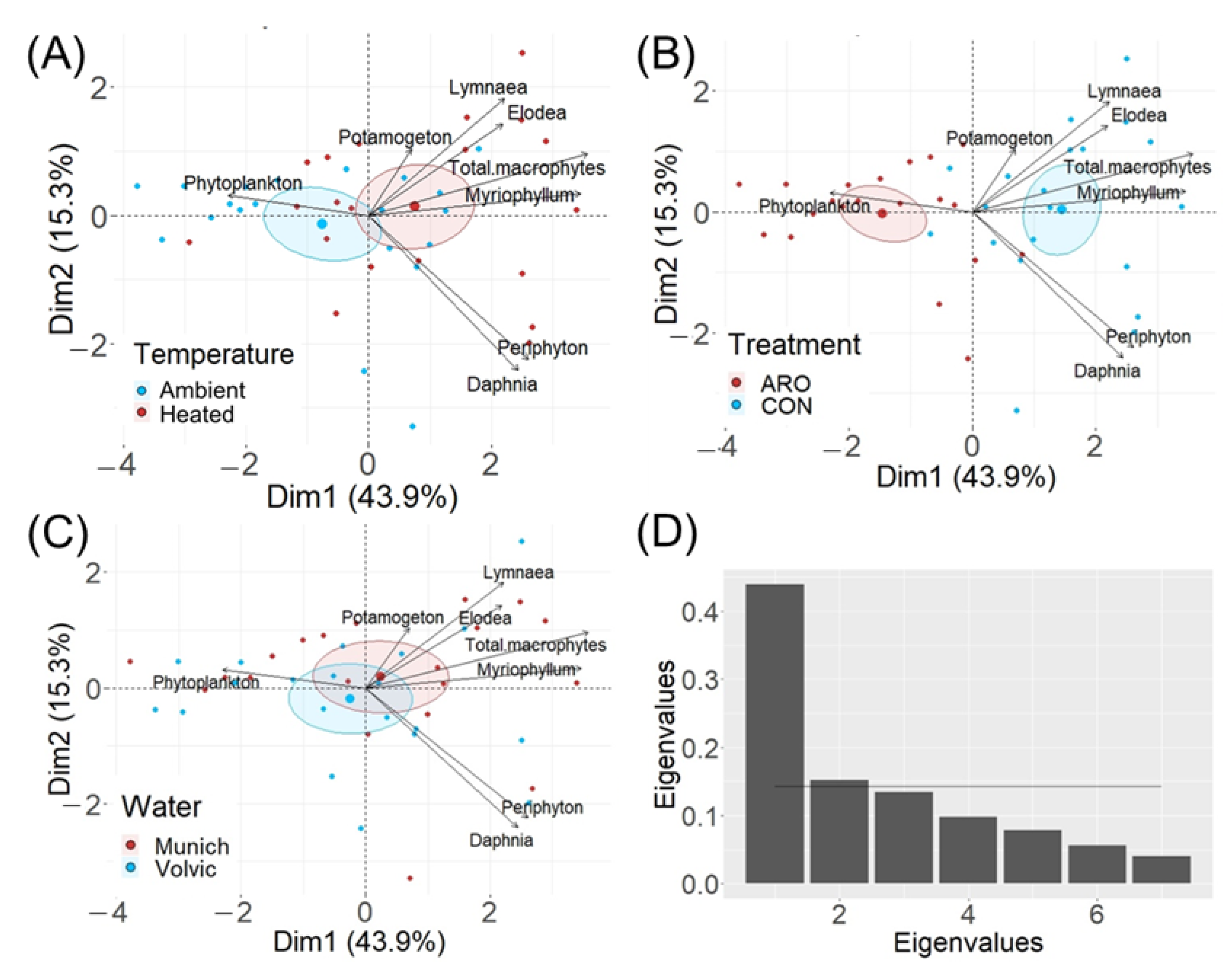
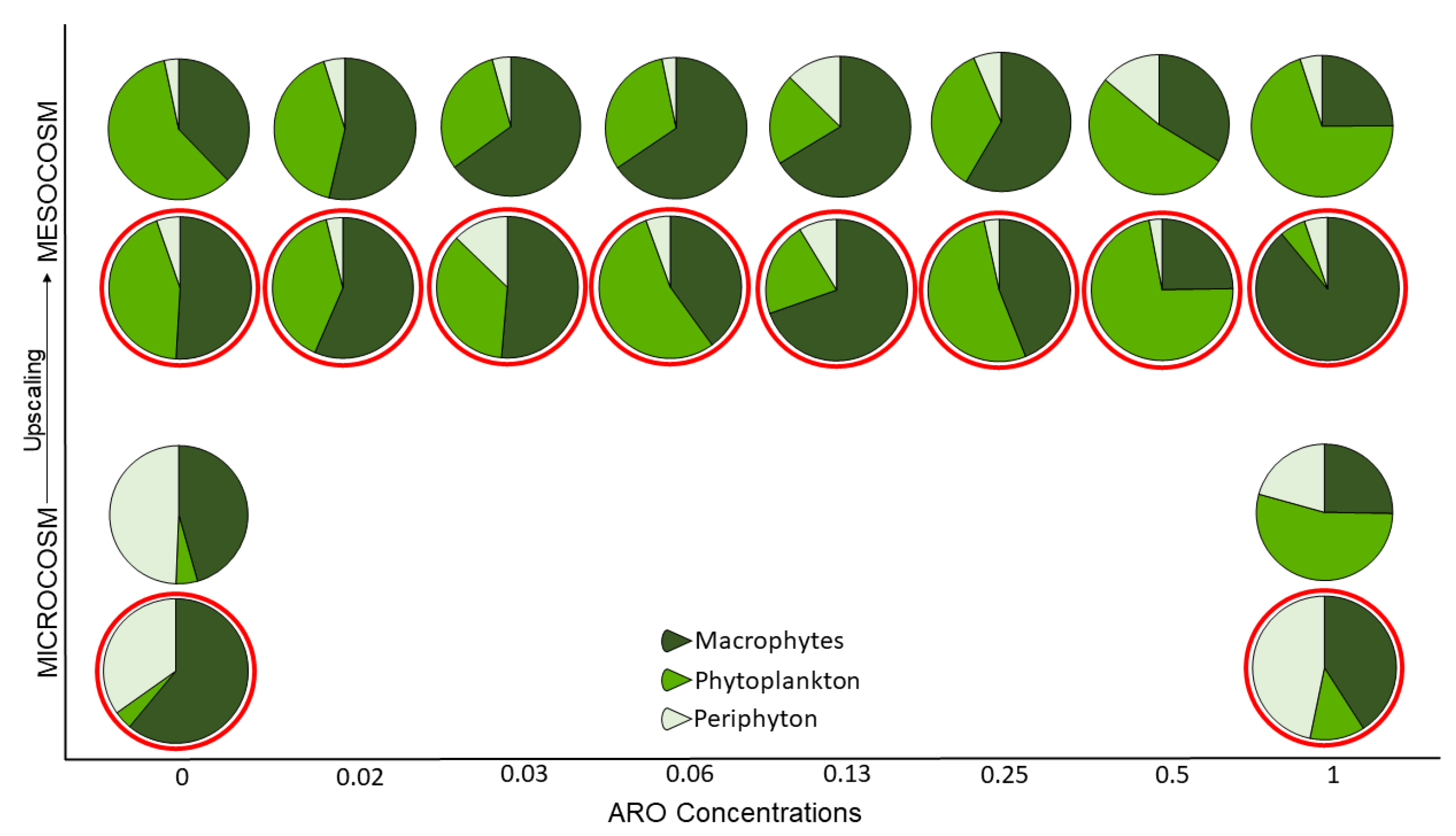
2.3. Comparison of the Primary Producer Community Structure in Micro- and Mesocosms
3. Results
3.1. Microcosm-Effects of Water Type
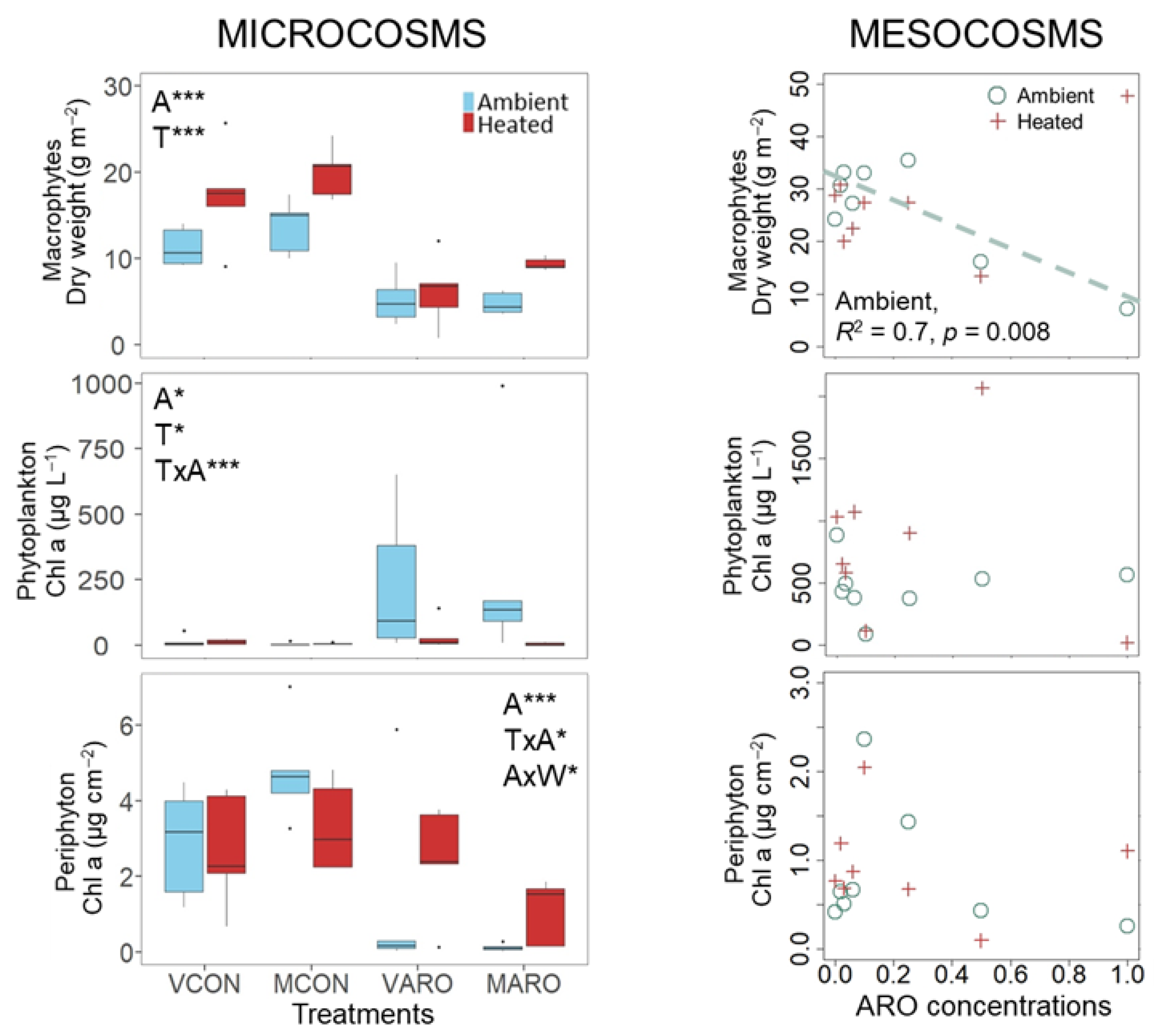
3.2. Stressor Effects on the Primary Producers
3.2.1. Microcosms
3.2.2. Mesocosms
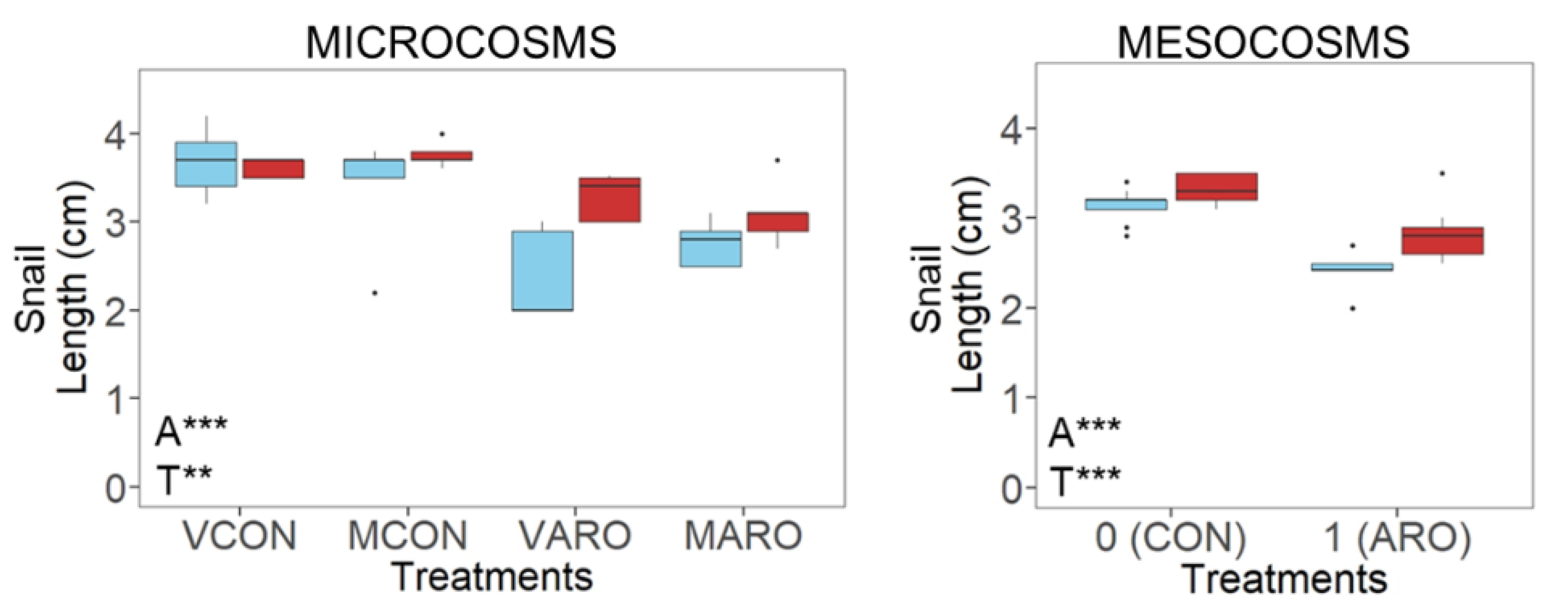
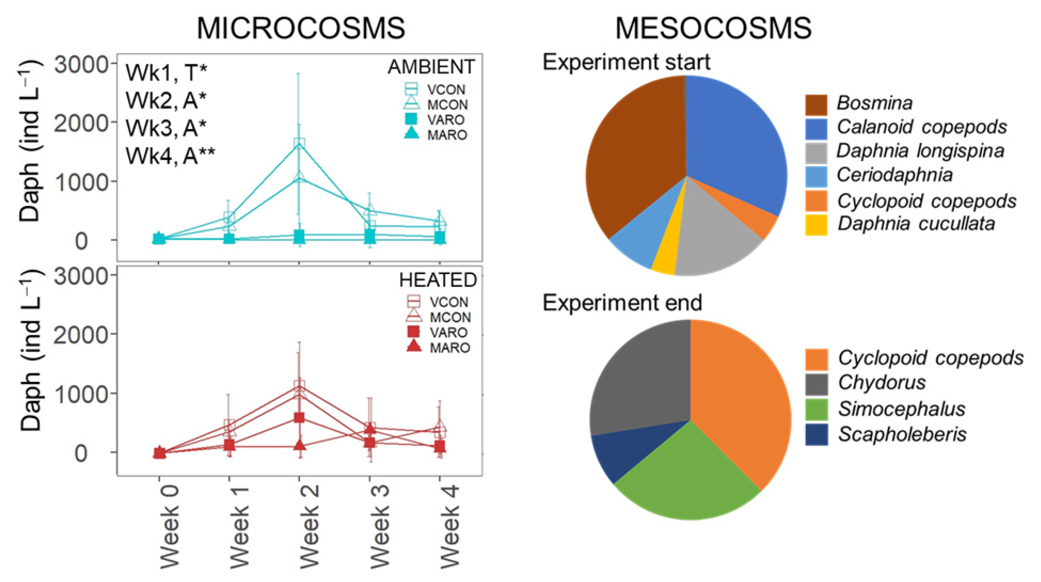
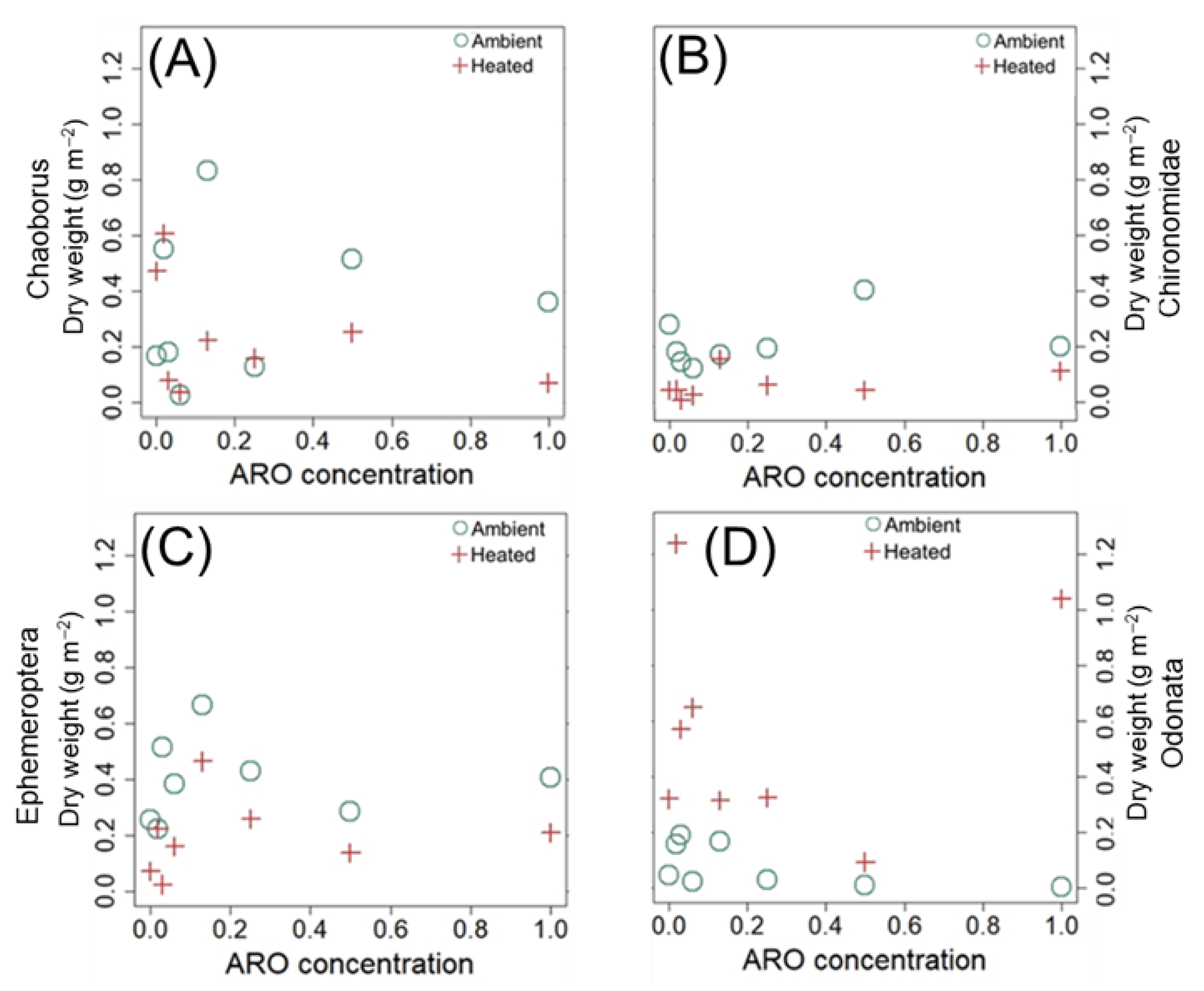
3.3. Stressor Effects on the Primary Consumers
3.3.1. Microcosms
3.3.2. Mesocosms
3.4. Regime Shifts in Micro- and Mesocosms
4. Discussion
4.1. The Role of Water Type in Upscaling Experiments
4.2. The Role of Community Complexity in Upscaling
4.3. The Role of Invasions in Upscaling
5. Conclusions
Supplementary Materials
Author Contributions
Funding
Data Availability Statement
Acknowledgments
Conflicts of Interest
References
- Scheffer, M.; Hosper, S.H.; Meijer, M.-L.; Moss, B.; Jeppesen, E. Alternative equilibria in shallow lakes. Trends Ecol. Evol. 1993, 8, 275–279. [Google Scholar] [CrossRef]
- Jeppesen, E.; Kronvang, B.; Meerhoff, M.; Søndergaard, M.; Hansen, K.M.; Andersen, H.E.; Lauridsen, T.L.; Liboriussen, L.; Beklioglu, M.; Özen, A.; et al. Climate Change Effects on Runoff, Catchment Phosphorus Loading and Lake Ecological State, and Potential Adaptations. J. Environ. Qual. 2009, 38, 1930–1941. [Google Scholar] [CrossRef] [PubMed]
- Barker, T.; Hatton, K.; O’Connor, M.; Connor, L.; Moss, B. Effects of nitrate load on submerged plant biomass and species richness: Results of a mesocosm experiment. Fundam. Appl. Limnol./Arch. Hydrobiol. 2008, 173, 89–100. [Google Scholar] [CrossRef]
- Moss, B.; Jeppesen, E.; Søndergaard, M.; Lauridsen, T.L.; Liu, Z. Nitrogen, macrophytes, shallow lakes and nutrient limitation: Resolution of a current controversy? Hydrobiologia 2013, 710, 3–21. [Google Scholar] [CrossRef]
- Sagrario, M.A.G.; Jeppesen, E.; Gomà, J.; Søndergaard, M.; Jensen, J.P.; Lauridsen, T.; Landkildehus, F. Does high nitrogen loading prevent clear-water conditions in shallow lakes at moderately high phosphorus concentrations? Freshw. Biol. 2005, 50, 27–41. [Google Scholar] [CrossRef]
- Colbourne, J.K.; Pfrender, M.E.; Gilbert, D.; Thomas, W.K.; Tucker, A.; Oakley, T.H.; Tokishita, S.; Aerts, A.; Arnold, G.J.; Basu, M.K.; et al. The Ecoresponsive Genome of Daphnia pulex. Science 2011, 331, 555–561. [Google Scholar] [CrossRef] [PubMed] [Green Version]
- OECD. Test No.211: Daphnia Magna Reproduction Test. 2012. Available online: https://www.oecd-ilibrary.org/content/publication/9789264185203-en (accessed on 18 December 2021).
- OECD. Test No.239: Water-Sediment Myriophyllum spicatum Toxicity Test. 2014. Available online: https://www.oecd-ilibrary.org/content/publication/9789264224155-en (accessed on 18 December 2021).
- Ebenebe, I.; Njemanze, I.; Ononye, B.; Ufele, A. Effect of Physicochemical Properties of Water on Aquatic Insect Communities of a Stream in Nnamdi. Int. J. Entomol. Res. 2019, 1, 2455–4758. [Google Scholar]
- Rameshkumar, S.; Radhakrishnan, K.; Aanand, S.; Rajaram, R. Influence of physicochemical water quality on aquatic macrophyte diversity in seasonal wetlands. Appl. Water Sci. 2019, 9, 12. [Google Scholar] [CrossRef]
- Gross, E.M.; Nuttens, A.; Paroshin, D.; Hussner, A. Sensitive response of sediment-grown Myriophyllum spicatum L. to arsenic pollution under different CO2 availability. Hydrobiologia 2018, 812, 177–191. [Google Scholar] [CrossRef]
- Potet, M.; Devin, S.; Pain-Devin, S.; Rousselle, P.; Giambérini, L. Integrated multi-biomarker responses in two dreissenid species following metal and thermal cross-stress. Environ. Pollut. 2016, 218, 39–49. [Google Scholar] [CrossRef]
- Davidson, T.A.; Audet, J.; Jeppesen, E.; Landkildehus, F.; Lauridsen, T.L.; Søndergaard, M.; Syväranta, J. Synergy between nutrients and warming enhances methane ebullition from experimental lakes. Nat. Clim. Chang. 2018, 8, 156–160. [Google Scholar] [CrossRef]
- Havens, K.E. An experimental comparison of the effects of two chemical stressors on a freshwater zooplankton assemblage. Environ. Pollut. 1994, 84, 245–251. [Google Scholar] [CrossRef]
- Landkildehus, F.; Søndergaard, M.L.; Beklioglu, M.; Adrian, R.; Angeler, D.; Hejzlar, J.; Papastergiadou, E.; Zingel, P.; Ayşe, I.; Cakiroglu, A.; et al. Climate change effects on shallow lakes: Design and preliminary results of a cross-European climate gradient mesocosm experiment. Est. J. Ecol. 2014, 63, 71–89. [Google Scholar] [CrossRef] [Green Version]
- Riis, T.; Olesen, A.; Jensen, S.; Alnoee, A.; Baattrup-Pedersen, A.; Lauridsen, T.; Sorrell, B. Submerged freshwater plant communities do not show species complementarity effect in wetland mesocosms. Biol. Lett. 2018, 14, 20180635. [Google Scholar] [CrossRef] [PubMed]
- Caquet, T.; Lagadic, L.; Monod, G.; Lacaze, J.C.; Couté, A. Variability of physicochemical and biological parameters between replicated outdoor freshwater lentic mesocosms. Ecotoxicology 2001, 10, 51–66. [Google Scholar] [CrossRef]
- Campbell, P.J.; Arnold, D.J.S.; Brock, T.C.M.; Grandy, N.J.; Heger, W.; Heimbach, F.; Maund, S.J.; Streloke, M. Higher-tier aquatic risk assessment for pesticides. In Proceedings of the Guidance Document from the SETAC-Europe/OECD/EC Workshop, Lacanau Océan, France, 19–22 April 1998. [Google Scholar]
- Pansch, C.; Hiebenthal, C. A new mesocosm system to study the effects of environmental variability on marine species and communities. Limnol. Oceanogr-Meth. 2019, 17, 145–162. [Google Scholar] [CrossRef]
- Watts, M.C.; Bigg, G.R. Modelling and the monitoring of mesocosm experiments: Two case studies. J. Plankton Res. 2001, 23, 1081–1093. [Google Scholar] [CrossRef] [Green Version]
- Kermoysan, G.; Pery, A.; Joachim, S.; Martz, V.; Miguet, P.; Porcher, J.-M.; Beaudouin, R. Variability in the outcome of outdoor mesocosms with three-spined Stickleback (Gasterosteus aculeatus) populations in control conditions: Data from 20 replicates in two annual experiments. In Proceedings of the SETAC Europe Annual Meeting “Securing a Sustainable Future: Integrating Science, Policy and People”, Berlin, Germany, 30 May 2012. [Google Scholar]
- Allen, J.; Gross, E.M.; Courcoul, C.; Bouletreau, S.; Compin, A.; Elger, A.; Ferriol, J.; Hilt, S.; Jassey, V.E.J.; Laviale, M.; et al. Disentangling the direct and indirect effects of agricultural runoff on freshwater ecosystems subject to global warming: A microcosm study. Water Res. 2021, 190, 116713. [Google Scholar] [CrossRef]
- Carrier-Belleau, C.; Drolet, D.; McKindsey, C.W.; Archambault, P. Environmental stressors, complex interactions and marine benthic communities’ responses. Sci. Rep. 2021, 11, 4194. [Google Scholar] [CrossRef]
- Wollrab, S.; Diehl, S.; De Roos, A.M. Simple rules describe bottom-up and top-down control in food webs with alternative energy pathways. Ecol. Lett. 2012, 15, 935–946. [Google Scholar] [CrossRef]
- Rippka, R.; Deruelles, J.; Waterbury, J.B.; Herdman, M.; Stanier, R.Y.Y. Generic assignments, strain histories and properties of pure cultures of cyanobacteria. Microbiology 1979, 111, 1–61. [Google Scholar] [CrossRef] [Green Version]
- Guillard, R.R.L.; Lorenzen, C.J. Yellow-green algae with chlorophyllide C. J. Phycol. 1972, 8, 10–14. [Google Scholar] [CrossRef]
- Pauw, N.D.; Laureys, P.; Morales, J. Mass cultivation of Daphnia magna Straus on ricebran. Aquac. Res. 1981, 25, 141–152. [Google Scholar] [CrossRef]
- R Core Team. R: A Language and Environment for Statistical Computing. R Foundation for Statistical Computing, Vienna. 2018. Available online: https://www.R-project.org (accessed on 18 December 2021).
- Lüdecke, D. Esc: Effect Size Computation for Meta Analysis (Version 0.5.1). 2019. Available online: https://CRAN.R-project.org/package=esc (accessed on 18 December 2021).
- Oksanen, J.; Blanchet, F.G.; Friendly, M.; Kindt, R.; Legendre, P.; McGlinn, D.; Minchin, P.R.; O’Hara, R.B.; Simpson, G.L.; Solymos, P.; et al. Vegan: Community Ecology Package (2.5-7). 2020. Available online: https://CRAN.R-project.org/package=vegan (accessed on 18 December 2021).
- Kassambara, A.; Mundt, F. Factoextra: Extract and Visualize the Results of Multivariate Data Analyses (1.0.7). 2020. Available online: https://CRAN.R-project.org/package=factoextra (accessed on 18 December 2021).
- Woitke, P.; Martin, C.-D.; Nicklisch, S.; Kohl, J.-G. HPLC determination of lipophilic photosynthetic pigments in algal cultures and lake water samples using a non-endcapped C18-RP-column. Fresenius J. Anal. Chem. 1994, 348, 762–768. [Google Scholar] [CrossRef]
- Schmitt-Jansen, M.; Altenburger, R. Community-level microalgal toxicity assessment by multiwavelength-excitation PAM fluorometry. Aquat. Toxicol. 2008, 86, 48–49. [Google Scholar] [CrossRef] [PubMed]
- Baldy, V.; Thiebaut, G.; Fernandez, C.; Mareckova, M.; Korboulewsky, N.; Monnier, Y.; Pérez, T.; Trémolieres, M. Experimental assessment of the water quality influence on the phosphorus uptake of an invasive aquatic plant: Biological responses throughout its phenological stage. PLoS ONE 2015, 10, e0118844. [Google Scholar] [CrossRef] [Green Version]
- Jones, J.; Eaton, J.; Hardwick, K. Physiological plasticity in Elodea nuttallii (Planch.) St. John. J. Aquat. Plant. Manag. 1993, 31, 88–94. [Google Scholar]
- Wacker, A.; Baur, B. Effects of protein and calcium concentrations of artificial diets on the growth and survival of the land snail Arianta Arbustorum. Invertebr. Reprod. Dev. 2004, 46, 47–53. [Google Scholar] [CrossRef]
- Polazzo, F.; Roth, S.K.; Hermann, M.; Mangold-Döring, A.; Rico, A.; Sobek, A.; Van den Brink, P.J.; Jackson, M.C. Combined effects of heatwaves and micropollutants on freshwater ecosystems: Towards an integrated assessment of extreme events in multiple stressors research. Glob. Chang. Biol. 2021, 28, 1248–1267. [Google Scholar] [CrossRef]
- Op de Beeck, L.; Verheyen, J.; Olsen, K.; Stoks, R. Negative effects of pesticides under global warming can be counteracted by a higher degradation rate and thermal adaptation. J. Appl. Ecol. 2017, 54, 1847–1855. [Google Scholar] [CrossRef] [Green Version]
- Loreau, M.; de Mazancourt, C. Biodiversity and ecosystem stability: A synthesis of underlying mechanisms. Ecol. Lett. 2013, 16 (Suppl. S1), 106–115. [Google Scholar] [CrossRef] [PubMed]
- Cottingham, K.L.; Knight, S.E.; Carpenter, S.R.; Cole, J.J.; Pace, M.L.; Wagner, A.E. Response of phytoplankton and bacteria to nutrients and zooplankton: A mesocosm experiment. J. Plankton Res. 1997, 19, 995–1010. [Google Scholar] [CrossRef] [Green Version]
- Mazumder, A. Phosphorus–chlorophyll relationships under contrasting zooplankton community structure: Potential mechanisms. Can. J. Fish. Aquat. 1994, 51, 401–407. [Google Scholar] [CrossRef]
- Du, X.; García-Berthou, E.; Wang, Q.; Liu, J.; Zhang, T.; Li, Z. Analyzing the importance of top-down and bottom-up controls in food webs of Chinese lakes through structural equation modeling. Aquat. Ecol. 2015, 49, 199–210. [Google Scholar] [CrossRef]
- Rose, V.; Rollwagen-Bollens, G.; Bollens, S.M.; Zimmerman, J. Effects of grazing and nutrients on phytoplankton blooms and microplankton assemblage structure in four temperate lakes spanning a eutrophication gradient. Water 2021, 13, 1085. [Google Scholar] [CrossRef]
- Carpenter, S.R.; Kitchell, J.F. Plankton community structure and limnetic primary production. Am. Nat. 1984, 124, 159–172. [Google Scholar] [CrossRef]
- Carpenter, S.R.; Kitchell, J.F.; Hodgson, J.R. Cascading trophic interactions and lake productivity. BioScience 1985, 35, 634–639. [Google Scholar] [CrossRef]
- Kuiper, J.; Altena, C.; Ruiter, P.; van Gerven, L.; Janse, J.; Mooij, W. Food-web stability signals critical transitions in temperate shallow lakes. Nat. Commun. 2015, 6, 7727. [Google Scholar] [CrossRef] [Green Version]
- Benke, A.C. Interactions among coexisting predators—A field experiment with dragonfly larvae. J. Anim. Ecol. 1978, 47, 335–350. [Google Scholar] [CrossRef]
- Hölker, F.; Vanni, M.; Kuiper, J.; Meile, C.; Grossart, H.-P.; Stief, P.; Adrian, R.; Lorke, A.; Dellwig, O.; Brand, A.; et al. Tube-dwelling invertebrates: Tiny ecosystem engineers have large effects in lake ecosystems. Ecol. Monogr. 2015, 85, 333–351. [Google Scholar] [CrossRef] [Green Version]
- Phillips, G.L.; Eminson, D.; Moss, B. A mechanism to account for macrophyte decline in progressively eutrophicated freshwaters. Aquat. Bot. 1978, 4, 103–126. [Google Scholar] [CrossRef]
- OECD. Test No.243: Lymnaea stagnalis Reproduction Test. Organisation for Economic Co-Operation and Development. 2016. Available online: https://www.oecd-ilibrary.org/environment/test-no-243-lymnaea-stagnalis-reproduction-test_9789264264335-en (accessed on 18 December 2021).
- Eriksson, B.K.; Rubach, A.; Batsleer, J.; Hillebrand, H. Cascading predator control interacts with productivity to determine the trophic level of biomass accumulation in a benthic food web. Ecol. Res. 2012, 27, 203–210. [Google Scholar] [CrossRef] [Green Version]
- Oksanen, L.; Fretwell, S.; Arruda, J.; Niemel. Exploitation ecosystems in gradients of primary productivity. Am. Nat. 1981, 118, 240–261. [Google Scholar] [CrossRef]
- Oksanen, L.; Oksanen, T. The logic and realism of the hypothesis of exploitation ecosystems. Am. Nat. 2000, 155, 703–723. [Google Scholar] [CrossRef] [PubMed]
- Abrams, P.A. Foraging time optimization and interactions in food webs. Am. Nat. 1984, 124, 80–96. [Google Scholar] [CrossRef]
- Levinton, J.S. Marine Biology: Function Biodiversity, Ecology, 5th ed.; Oxford University Press: New York, NY, USA, 1995; pp. 46–72. [Google Scholar]
- Janssen, A.B.G.; Hilt, S.; Kosten, S.; de Klein, J.J.M.; Paerl, H.W.; de Waal, D.B.V. Shifting states, shifting services: Linking regime shifts to changes in ecosystem services of shallow lakes. Freshw. Biol. 2021, 66, 1–12. [Google Scholar] [CrossRef]


Publisher’s Note: MDPI stays neutral with regard to jurisdictional claims in published maps and institutional affiliations. |
© 2022 by the authors. Licensee MDPI, Basel, Switzerland. This article is an open access article distributed under the terms and conditions of the Creative Commons Attribution (CC BY) license (https://creativecommons.org/licenses/by/4.0/).
Share and Cite
Vijayaraj, V.; Kipferler, N.; Stibor, H.; Allen, J.; Hölker, F.; Laviale, M.; Leflaive, J.; López Moreira Mazacotte, G.A.; Polst, B.H.; Schmitt-Jansen, M.; et al. Evaluating Multiple Stressor Effects on Benthic–Pelagic Freshwater Communities in Systems of Different Complexities: Challenges in Upscaling. Water 2022, 14, 581. https://doi.org/10.3390/w14040581
Vijayaraj V, Kipferler N, Stibor H, Allen J, Hölker F, Laviale M, Leflaive J, López Moreira Mazacotte GA, Polst BH, Schmitt-Jansen M, et al. Evaluating Multiple Stressor Effects on Benthic–Pelagic Freshwater Communities in Systems of Different Complexities: Challenges in Upscaling. Water. 2022; 14(4):581. https://doi.org/10.3390/w14040581
Chicago/Turabian StyleVijayaraj, Vinita, Nora Kipferler, Herwig Stibor, Joey Allen, Franz Hölker, Martin Laviale, Joséphine Leflaive, Gregorio Alejandro López Moreira Mazacotte, Bastian Herbert Polst, Mechthild Schmitt-Jansen, and et al. 2022. "Evaluating Multiple Stressor Effects on Benthic–Pelagic Freshwater Communities in Systems of Different Complexities: Challenges in Upscaling" Water 14, no. 4: 581. https://doi.org/10.3390/w14040581