
Modelling Intense Combined Load Transport in Open Channel


Faculty of Civil Engineering, Czech Technical University in Prague, 166 29 Prague, Czech Republic
Water 2022, 14(4), 572; https://doi.org/10.3390/w14040572
Submission received: 21 December 2021
/
Revised: 8 February 2022
/
Accepted: 11 February 2022
/
Published: 14 February 2022
(This article belongs to the Special Issue Granular Flows Modeling and Simulation)
Abstract
:Granular flow is modelled under the following conditions: Steady-state uniform turbulent open-channel solid–liquid flow carrying combined load at high solids concentration above a plane mobile bed. In the combined load, a portion of transported particles is transported as collisional bed load and the rest as suspended load supported by carrier turbulence. In our modelling approach, we consider one-dimensional flow and take into account a layered structure of the flow with the intense combined load. Principles of kinetic theory of granular flow are employed together with the mixing-length theory of flow turbulence in order to predict distributions of solids concentration and velocity in sediment-water flow of the given flow depth and longitudinal slope in an open channel. Components of the model are tested and calibrated by results of our laboratory experiments with lightweight sediment in a recirculating tilting flume.
1. Introduction
In an open channel with a mobile bed composed of loose sediment particles, flow of water interacts with the top of the bed and the interaction causes transport of sediment provided that a bed shear criterion for transport is satisfied [1]. In steep streams and high flow rates, bed shearing can become so intense that the induced flow rate of transported sediment becomes a considerable portion of the total flow rate of mixture of water and sediment in the channel. Depending on flow conditions and properties of sediment particles, the particles are transported either as bed load, or as suspended load or as combined load [2]. In transport of bed load (contact load), sediment particles are supported predominantly by mutual contacts, while particles transported as suspended load interact with flowing carrier instead of other particles and carrier turbulence keeps them suspended in the flow. In transport of combined load, both support mechanisms are effective, a part of transported particles is supported by contacts (often dominantly collisions) and the rest is suspended by turbulence. Due to variability of local conditions along the flow depth, the combined load transport can occur even if particles of the same size and density are transported in the flow.
Flow with intense transport of sediment tends to develop a layered structure across the flow depth as observed in laboratory experiments [3,4]. In such a flow of high-concentrated mixture, sediment particles are non-uniformly distributed across the flow depth above a typically plane top of the bed. Dominating mechanisms of particle support are different in the different layers and affect their thickness. For engineering purposes, a modelling approach to transport of sediment has been primarily empirical and produced transport correlations relating the sediment flow rate with the flow depth and the channel longitudinal slope without considering the internal structure of the flow. However, information about the structure and its exploration in modelling of the sediment transport is important to make model results more complete and physically sound.
Detailed experimental studies which include information on the internal structure of mixture flow (basically information on distributions of sediment concentration and velocity across the flow depth) with intense sediment transport over an erodible plane bed are scarce. More information is available for pressurized flows than for flows in open channels. In a pressurized pipe, the high bed shear condition at the top of stationary deposit is easy to reach due to the high hydraulic gradient i (frictional head loss over a unit length of a pipe), , where τ0 is the bed shear stress, ρf is the fluid density, g is the gravitational acceleration and Rh0 is the hydraulic radius of the bed associated area of a flow cross section [5]. An ability of flow to transport a solid particle is evaluated using the bed Shields parameter θ0, which the ratio of the shear force exerted by fluid on the particle and the submerged weight of the particle, , where ρs is the solids density and d is the particle size. In pressurized flows, transport of solids is typically very intense, with the maximum volumetric flow rate of solids exceeding 25 per cent of the total flow rate of mixture [6]. For laboratory pipes, various measuring techniques to sense distributions in a pipe cross section have been available, for instance, a radiometric profiler for a concentration distribution [5,6,7]. Results of pipe experiments were used primarily to evaluate the friction condition at the top of the erodible bed at high bed shear and resulted in relationships between the bed friction coefficient and the bed roughness modified to include the interaction of transported sediment with the bed surface [5,8,9]. Furthermore, the pipe experiments, which typically cover a broad range of bed shear conditions, were exploited to define different modes of sediment transport. The widely used approximate criterion, based on a pressurized-pipe experiment, requires that the suspension ratio, i.e., the ratio of the bed shear velocity, , and the terminal settling velocity of a particle, exceeds 1 (or 1.25) to enable transport of particles in the turbulent suspension mode [8]. For lower values of the suspension ratio, the non-suspension mode (basically contact-load transport) dominates.
Flume experiments on the internal structure of flow with intense sediment transport are currently more common as appropriate measuring techniques have become available recently for open channel flows of relatively high concentrated solid–liquid mixtures. Camera-based measuring techniques rely on tracking of particles in a near-wall domain of the flow to extract their local velocities [10,11] and concentrations [12] from a sequence of flow images recorded through a glass wall of a flume. So far, experiments exploiting these techniques targeted primarily purely collisional (bed-load) granular flows [3,13,14,15] covering a relatively broad range of bed shear conditions.
An alternative measuring principle, based on the acoustic Doppler effect, is employed by a measuring instrument ACVP to measure simultaneously profiles of velocity and concentration of particles across the depth of sediment-laden flow [4]. The instrument’s high resolution and frequency enables to quantify local turbulent characteristics and an analysis of measured local parameters allows for an identification of layers in flow with intense sediment transport [4]. So far, few test runs have been reported for very similar bed shear conditions.
Modelling efforts taking the internal structure of intense sediment transport into account have intensified recently. Works focus on CFD numerical two-phase models, e.g., [16,17], and alternatively on less computationally challenging algebraic models considering one-dimensional steady uniform flow. The latter models exploit principles of kinetic theory of granular flows and are therefore very suitable for a description of collision dominated transport [3,13,15,18,19]. The kinetic theory provides constitutive formulae which can be exploited to mutually relate distributions of local stresses, concentrations and velocities of colliding particles. In the models, the constitutive relations are combined with momentum balance equations for solids and mixture to provide relations among global quantities describing flow and transport (flow rates of mixture and its phases, the flow depth and the longitudinal slope). Current kinetic-theory based contact-load models assume linear distributions of velocity and concentration across the collisional transport layer and the uniform distribution of velocity in the water layer above the transport layer [3,15,19]. If the additional dense sliding layer is considered below the collisional transport layer, then it exhibits uniform distributions of concentration and velocity [18,19]. Basically, the existing models differ in chosen forms of constitutive relations and in assumptions made for conditions at flow interfaces.
A kinetic-theory based transport model is applicable to flow with combined load transport if modifications are introduced to account for the ability of carrying liquid to suspend transported sediment particles. A principle of the turbulent support of particles assumes that the submerged weight of a burden of sediment at a certain position within a transport layer is either entirely or partially balanced by a lift force produced by a diffusive action of turbulent eddies on the particles in the layer. The lifting effect is described by a turbulent diffusion equation based on a balance of granular fluxes due to particle settling and particle dispersion as in the theory by Rouse and Schmidt (e.g., [20,21]). An evaluation of the turbulent diffusive action requires a local characterization of carrier turbulence and is done by using the Prandtl mixing-length theory in the Rouse–Schmidt concept.
So far, kinetic-theory based combined-load transport models similar to those for contact-load transport have been proposed only for pressurized flows [22,23]. They consider the transport layer divided into two parts—the upper suspended-load layer, in which particles interact exclusively with the eddies, and the lower turbulent collisional layer, in which a portion of particles is supported by turbulent eddies and the rest by collisions. To account for the lift effect, the turbulent-diffusion term is included in the momentum balance equation for the local granular normal stress at the bottom of the collisional layer. The model by Berzi and Fraccarollo [23] applies the suspension-ratio criterion from [8] to identify the top of the suspended-load layer (called fully turbulent layer by Berzi and Fraccarollo) at which the fluid shear stress has the minimum value required to suspend transported particles. The fluid shear stress exceeds this threshold stress throughout the fully turbulent layer and reaches a value equal to the flow induced total shear stress (a value of Shields parameter) at the bottom of the layer. The same total shear stress is assumed to act at all elevations between this interface and the top of the bed. In the model, the mixing length l is assumed to increase linearly with the distance from the top of stationary deposit y (l = κy, where κ is von Karman constant). The distribution of velocity is linear across the dense layer and the adjacent turbulent collisional layer and it is uniform at elevations above the top of the turbulent collisional layer. The distribution of concentration is linear in the dense layer and in the turbulent collisional layer and it is non-linear, following the Rouse–Schmidt solution, above the top of the turbulent collisional layer.
Our previous work was concerned with intense transport of contact load dominated by intergranular collisions. We built our experimental database of results for contact-load transport of lightweight sediments in a laboratory tilting flume [24,25,26] and used it to test constitutive relations of the classical kinetic theory and the extended kinetic theory at conditions typical for intense contact-load transport [25]. Selected constitutive relations based on the classical kinetic theory were employed in a collisional transport model for intense bed load in open-channel flow [27]. For given slope and depth of the flow, the model predicts the total flow rate and the flow rate of sediment while considering the internal structure of the flow described by linear vertical distributions of velocity and concentration across the collisional layer. In [28], we tested which criteria are suitable to assess whether collisional contact is a dominating particle-support mechanism at various elevations within a transport layer of our observed flows. We exploited experimental data at flow conditions where the transition between predominantly contact load and predominantly suspended load were most likely to occur. For selected tests, experimentally observed distributions of velocity and concentration enabled to evaluate relevant turbulence-associated quantities, as the mixing length, at various vertical positions in the transport layer. A distribution of the mixing length was extracted from the experimental data using two alternative approaches. One approach isolated the local mixing length from the Rouse–Schmidt equation and the other from a Karman-constant containing formula suitable for a transport-layer condition [4]. The latter equation includes the turbulence damping effect quantified using Richardson number. It modifies the local mixing length in flow exhibiting steep gradients of local velocity and concentration, which is a condition typical for a transport layer. The mixing length from the turbulent-diffusion equation is interpreted as the local mixing length required to maintain particles suspended at the local position. It is assumed that this length must be bigger than the available mixing length at the position. This mixing length is related to the local flow conditions and determined by the equation with the Richardson number. Furthermore, the local mixing length should be bigger than the particle size to ensure that turbulent eddies are able to suspend the particles. It appeared that the assumptions were satisfied in the upper part of a transport layer if the bed Shields parameter exceeded say 1.5 (corresponding with the suspension ratio of about 1.2) and so showed that the threshold at which a relevant part of the transport layer exhibited turbulent suspension of particles corresponded well with the suspension-ratio criterion from [8]. This analysis provided information which could be further exploited in a development of a combined-load transport model for open-channel flow.
The main aim of the work reported in this paper is to develop a transport model for open-channel flow with intense combined load which includes predictions of profiles of velocity and concentration across the flow depth, and predictions of other relevant quantities at all interfaces of the layered structure of the sediment laden flow. The model should be simple enough to be easily applicable for engineering purposes. Moreover, the model should contribute to a further refinement of combined-load modelling options offered by the previous models designed for pressurized flows, e.g., by modifications of some simplifying assumptions regarding distributions of relevant quantities (shear stress, mixing length, velocity).
The additional major objective of this work is to calibrate model components and to validate the model by new original experimental results produced in our laboratory flume. So far, no suitable experimental data covering a required sufficiently broad range of the combined-load transport conditions and including the distributions of concentration and velocity have been made available.
2. Materials and Methods
A modelling approach is employed which enables to predict characteristics of fully developed steady uniform turbulent open-channel flow with intense transport of combined load. The approach is based on appropriate theories and considers a layered structure of the sediment-laden flow. The resulting transport model considers conditions at identified layer interfaces and conditions within individual layers to simulate mutual relations among the longitudinal slope, flow depth and distributions of velocity and concentration of sediment.
The transport model is calibrated and validated by own experiments which produced sufficiently detailed information about tested flow conditions including measured profiles of sediment concentration and velocity.
2.1. Combined-Load Model
2.1.1. Modelled Conditions
The modelled solid–liquid flow is a one-dimensional inclined gravity-driven open-channel flow with intense transport of sediment over an erodible bed with a plane surface. Above the bed, the flow is composed of layers in which different dominating mechanisms of particle support act and it results in different distributions of velocity and concentration across the different layers. Based on these assumptions, different theories and equations are applied in the individual layers and at their interfaces.
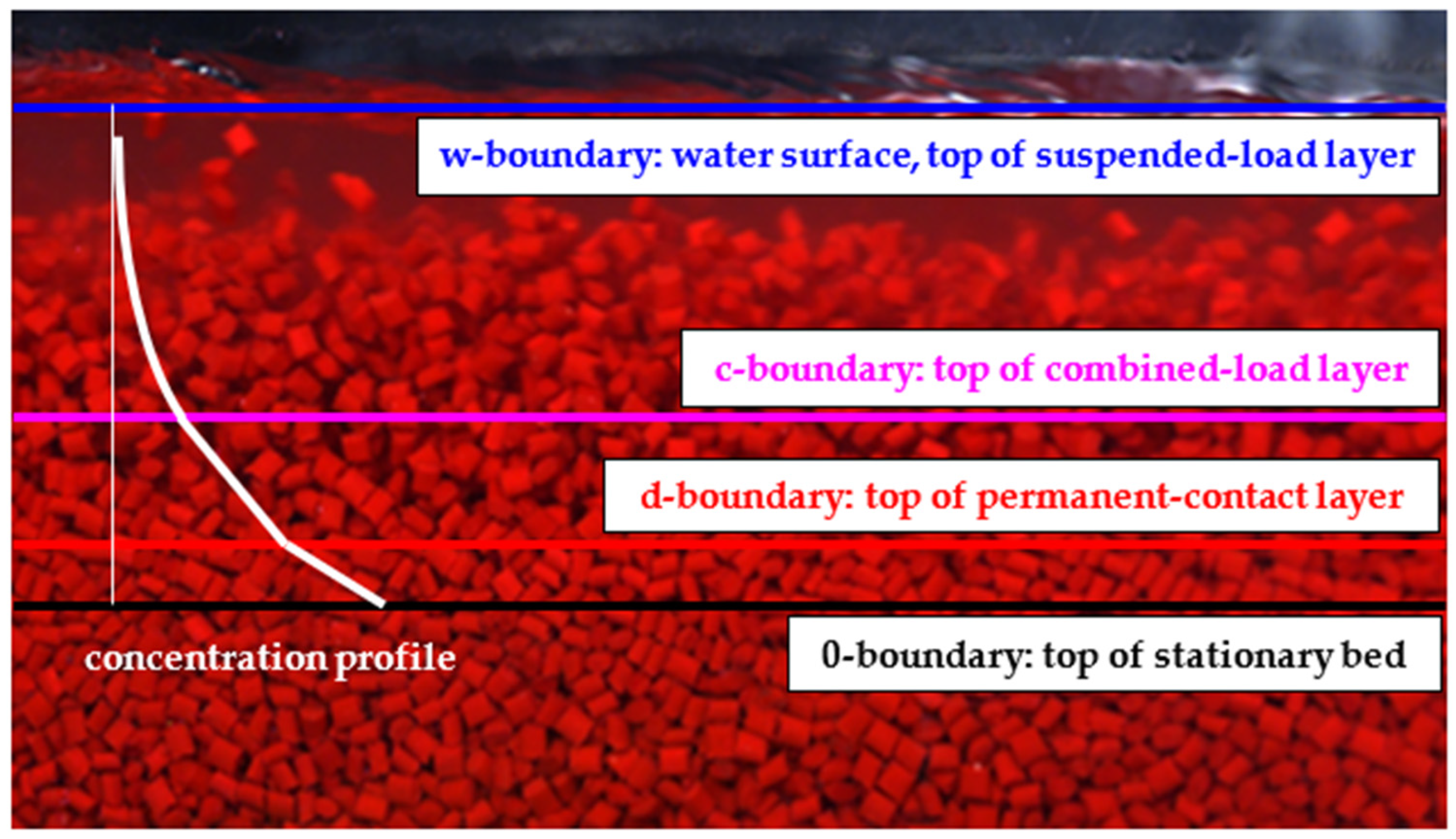
The assumed layers and interfaces are (Figure 1):
- The stationary bed (granular deposit with the plane surface expressed as the 0-boundary);
- the permanent-contact (dense sliding) layer (its top is the d-boundary);
- the combined-load (collision and turbulent suspension) layer (its top is the c-boundary);
- the suspended-load (turbulent suspension) layer (its top is the water surface, the w-boundary).
2.1.2. Model Assumptions
Specific assumptions are proposed for the individual layers and their boundaries to emphasize dominating conditions and mechanisms and at the same time to simplify the conditions so that an analytical solution of the model is feasible. Some assumptions originate from experimental experience with the modelled type of solid–liquid flow.
In the permanent-contact layer (the d-layer), the local volumetric concentration of solids c is higher than the maximum concentration to which constitutive relations of the classical kinetic theory apply. The submerged weight of transported particles is assumed to be supported solely by interparticle contact which is virtually permanent. The granular body is sheared and hence there is a velocity gradient throughout the layer which is maximum at the top of the layer and tends to zero at the bottom. The solids distribution is not uniform across the layer either with the local concentration at the bottom of the layer (the bed concentration c0, here and below an index indicates the position at which the quantity is evaluated) being larger than the concentration at the top of the layer cd. This lower concentration at the top is responsible for a predominantly collisional contact among particles at this interface. Hence, the support of particles is assumed to be purely collisional at the d-boundary and this boundary is the lowest elevation at which the collisional contact applies.
Above this interface, i.e., in the regions occupied by the combined-load layer and the suspended-load layer, turbulent lift contributes to balance the submerged weight of the particles in the direction perpendicular to the interface. In the combined-load layer (the c-layer), both particle support mechanisms (collision and turbulent lift) act at each elevation with the increasing contribution of turbulent suspension at higher elevations in the layer. At the top of the combined layer the collisional support vanishes. Our experiments (discussed below) suggest that distributions of both concentration and velocity are virtually linear across the layer as is the case with purely collisional transport layers investigated previously [24,25,26].
In the suspended-load layer (the s-layer) adjacent to the top of the combined-load layer, the distributions are no longer linear, and their shape is governed by turbulent diffusion which is no longer affected by colliding particles [29] as is the case in the combined-load layer. All particles are suspended by the lifting action of turbulent fluctuating velocities of carrying fluid.
Throughout all layers, the local velocities u and their gradients γ are assumed to be equal for liquid and sediment. Previous investigations justify this assumption through experimental evidence [26] and theoretical analysis [30]. The analysis showed that even a very small difference in local velocities of solids and fluid produces a sufficiently large drag force on particles in a transport layer of inertial flow.
2.1.3. Model Principles and Applied Theoretical Concepts
The modelled flow conditions require to simulate a flow behavior of solid–liquid mixture in which interactions between the two phases (solid–liquid interaction) and interactions among transported solid particles (particle–particle interaction) are equally important. The particle–particle interactions are either sporadic although intense (collisions) or permanent (sliding contact). Particle-fluid interactions include buoyancy, drag and turbulent lift. The last is active only if appropriate conditions are satisfied.
The particle–particle interactions are described using principles of the kinetic theory of granular flows. It exploits constitutive relations for local particle stresses (normal and shear) and for a balance of particle fluctuation energy resulting from interparticle collisions in a sheared granular body. The classical kinetic theory considers that particles interact exclusively by mutual binary collisions which covers collision-driven transport of particles at low to moderate local concentrations and where particles exchange momentum through uncorrelated collisions, e.g., [3,13,15]. The extended kinetic theory covers correlated motion of particles in the environment of high local concentration of particles and modifies the constitutive relations for the condition called the dense limit, e.g., [18,19]. The threshold concentration at which relations of the classical theory cease holding because particle velocity fluctuations due to collisions begin to be correlated is called the freeze concentration (cf).
The mixing-length concept based on the Prandtl theory is exploited to solve the distributions of velocity and fluid shear stress in the suspended-load layer. In the model, the effect of the gradients of concentration and velocity on the local mixing length using Richardson number is applied as in [4]. Furthermore, the distribution of the mixing length is used to describe interactions of suspended particles with turbulent eddies for purposes of a determination of distribution of sediment concentration in the suspended-load layer using the turbulent diffusion concept with the Rouse–Schmidt formula. In high concentrated flows like flows with intense transport of sediment, the local terminal settling velocity of a particle should include a hindered settling term by Richardson and Zaki [22,23] and it is included in the model.
Furthermore, the mixing-length concept is exploited to express fluid turbulence suppression due to the presence of colliding particles [29] inside the combined-load layer. In the flow with colliding particles, the local mixing length depends on the mean distance between particles at the location and hence decreases with the increasing local concentration of solids towards the bottom of the layer. It results in diminishing of the local effective viscosity relating the turbulent fluid stress with the fluid shear rate. Furthermore, the local fluid effective viscosity has an additional granular-like component related to the exchange of momentum between the fluid shells surrounding the fluctuating particles and it can be expressed as added-mass effect [29] using the added mass term introduced to constitutive relations by [13]. In the model calculations, the suppression of turbulence diminishes the fluid shear stress at the d-boundary and affects the thickness of the d-layer.
2.1.4. Model Features
The model exploits momentum balances to relate stresses at different interfaces. Furthermore, the model exploits constitutive relations by Garzó and Dufty [31] simplified to conditions at dense limit with the freeze concentration at the d-boundary [32]. The constitutive relations take care of local stresses and other relevant parameters at the d-boundary and assist to determine the elevation of the d-boundary, yd (y is the distance from the top of the bed in the direction perpendicular to the bed). Above the d-boundary, the applied assumptions (including experiment-based ones) enable to abandon the constitutive relations and to simulate the flow exclusively using a combination of momentum balance and particle-fluid interactions.
The model requires input information on properties of liquid (density ρf and dynamic viscosity μf) and sediment (density ρs, equivalent diameter d and terminal settling velocity w) and on flow (the depth H and the longitudinal slope ω). It employs constants related to constitutive relations (bed concentration c0, concentration at d-boundary cd, effective coefficient of restitution of particles in dry conditions ε, particulate friction coefficient at the bed β0, constant for solids stress ratio at the d-boundary Cbd) and to turbulent-diffusivity relations (von Karman constant κ, constant for initial mixing-length position Cini, particle diffusivity constant Cη). The model predicts elevations of the d-boundary, c-boundary and distributions of concentration and velocity as major outputs.
- Inputs: Solid/liquid properties: d, ρs, w, ρf, μf
- Flow: H, ω
- Constants: c0, cd, ε, β0, κ, Cbd, Cini, Cη
- Major outputs: Positions of interfaces between layers: yd, yc
- Distributions of velocity and solids concentration in layers: u(y), c(y)
2.1.5. Model Equations and Computational Procedure
An analytical solution of the combined-load transport model is described below in a step-by-step procedure using equations in their final form based on applied conditions. The general assumptions have already been discussed; more specific assumptions are added below where appropriate. Some described equations are the same as in previously published collisional-transport models and they are derived elsewhere. References are added to appropriate sources.
In the equations below, all quantities are dimensionless. The conversion to their dimensional counterparts using g, d, ρs, ρf and the specific gravity S = ρs/ρf is summarized in Appendix A. The notation of dimensionless quantities and corresponding dimensional quantities is the same for sake of simplicity.
The permanent-contact (dense sliding) layer (the d-layer and its boundaries: The d-boundary, the 0-boundary).
As the first step, a value of the coefficient of wet restitution ed (subject to iteration in the procedure) is introduced. The coefficient e differs from ε by the additional damping effect of lubrication forces on collisions expressed through the fluid dynamic viscosity, μf, and the granular temperature, T (a measure of local particle velocity fluctuations due to intergranular collisions) [18]. In the procedure, the introduction of ed enables to express Td at the d-boundary as in [19]
where is particle Reynolds number.
It is assumed that turbulence does not suspend any particles at the d-boundary. All particles are supported by collisions and particle velocity fluctuations begin to be correlated at this boundary. Hence, constitutive relations of the extended kinetic theory apply and the one for the solids normal stress (s-index for solids) reads
in which the radial distribution function at contact for dense limit [32]
where ccr is the critical concentration and cf is the freeze concentration (we assume cd = cf).
The solid stress ratio βd can be isolated from the constitutive relation expressing the balance of fluctuation energy of colliding particles for the assumption of negligible diffusion flux in the energy balance as in [19]
in which the concentration-related function by Garzó and Dufty [31] for dense limit [19]
and the correlation length Ld = 1. For calculating the solids shear stress at the d-boundary using the stress ratio βd, it appeared necessary to expand the relation with the empirical constant Cβd which in a simplistic way compensated for effects not included in the constitutive relation. This compensation was required to match a predicted velocity gradient with an experimentally determined velocity gradient across the combined-load layer which was considered constant across the entire layer. The effects not covered by the used constitutive relation may include the effect of the diffusion flux (neglected in the balance above) and/or the effect of inhomogeneity (non-uniform distribution of sediment and only partial collisional suspension above the interface) on the solids shear stress. Thus
The local shear-induced solids shear stress, τs, is also related to local c and T in a constitutive relation for the shear stress which relates τs to the local solids shear rate γs (the gradient of longitudinal velocity u) [18]. This information enables to express the shear rate at the d-boundary
The local fluid shear stress τf (f-index for fluid) is related to the local fluid shear rate through the local fluid effective viscosity. Note that the shear rates are assumed to be equal for liquid and solids at any elevation in the flow (γ = γf = γs). Following [29], the local fluid effective viscosity at the d-boundary is split into two components
The granular-like component is proportional to the particle viscosity,, and the added-mass term ad,
where from [13]
It is assumed that the turbulent component of the local effective viscosity, associated with the local mixing length, is negligible at the d-boundary, , and therefore
A relationship determining the elevation of the top of the dense sliding layer (i.e., also the thickness of the dense sliding layer) is obtained from the stress balance at the 0-boundary expressed by a combination of momentum balances and constitutive relations and it reads
This thickness is required together with the information about the distribution of the shear rate across the d-layer (assumingly linear) and the shear rate at the bottom of the layer (γ0 = 0) to determine the velocity at the top of the layer
At the 0-boundary, velocity is neglected (u0 = 0) and so is the fluid shear stress (τf0 = 0). The solids shear stress is related to the solids normal stress through the yielding value given by the coefficient β0. The normal stress is obtained from the momentum balance
and thus
The resulting bed Shields parameter
is compared with a value of the bed Shields parameter obtained from the flow quantities which are inputs to the model (the flow depth H and the slope ω)
in which the effect of mixture density on the Shields parameter is neglected. This is justified by the low value of S of the lightweight sediment which produces low values of the specific gravity of mixture. In the procedure, the condition selects a value of ed for which values of other quantities at the d-boundary are determined.
Finally, the profiles of velocity and concentration are calculated for the conditions of a linear distribution of the shear rate and of a uniform distribution of the concentration gradient throughout the d-layer
The combined-load (collisional and suspended) layer (the c-layer, the c-boundary).
In the c-layer, a certain part of transported particles exchanges momentum through uncorrelated collisions. At the top of the c-layer, the concentration of colliding particles and the particle stresses vanish. The gradients are assumed constant across the c-layer. At the top of the c-layer, the velocity gradient , and the concentration gradient
This determines a value of Richardson number at the top of the c-layer
and it is further used to identify the mixing length at the c-boundary [4]
in which the initial position yini is estimated as a multiple of the thickness of the d-layer, , and a value of Cini is calibrated by experiments. The liquid shear stress at the c-boundary
where the effective viscosity equals to the local turbulent viscosity (the granular viscosity does not apply due to the absence of colliding particles) [29],
Moreover, the fluid shear stress can be expressed by the momentum balance at the c-boundary
and a combination of the two equations for the local fluid shear stress determines the position of the top of the combined-load layer, yc.
The local concentration at this boundary, cc, is obtained from the turbulent diffusion balance (Schmidt–Rouse equation). Its use is justified by the assumption that all particles are suspended by turbulence at this elevation,
The equation is solved iteratively for cc. The velocity at the top of the c-layer is determined simply from the assumption of the linear distribution of velocity across the c-layer
The profiles of velocity and concentration throughout the c-layer,
The suspended-load (turbulent suspension) layer (the s-layer, the w-boundary).
Near the top of the s-layer, particles are often absent, and the solids concentration tends to zero. At the top of the layer, i.e., at the water surface, the liquid shear stress vanishes. The profile of velocity is obtained from the logarithmic equation using the boundary condition at the c-boundary,
The concentration profile is obtained from the set of equations below:
in which the effect of mixture density is neglected, , , and .
If these equations are combined, then they produce one implicit relationship
Equation (22) is solved iteratively to get c at any elevation y inside the s-layer for estimated gradient (c−1, y−1 being values at the previous elevation).
This completes the calculation procedure and the resulting layered structure of flow can be plotted including the positions of the boundaries of the individual layers and the distributions of velocity and solids concentrations across all layers. Those are further compared with experimentally determined profiles of velocity and concentration obtained from laboratory experiments described below.
2.2. Experimental Work
2.2.1. Experimental Set-Up
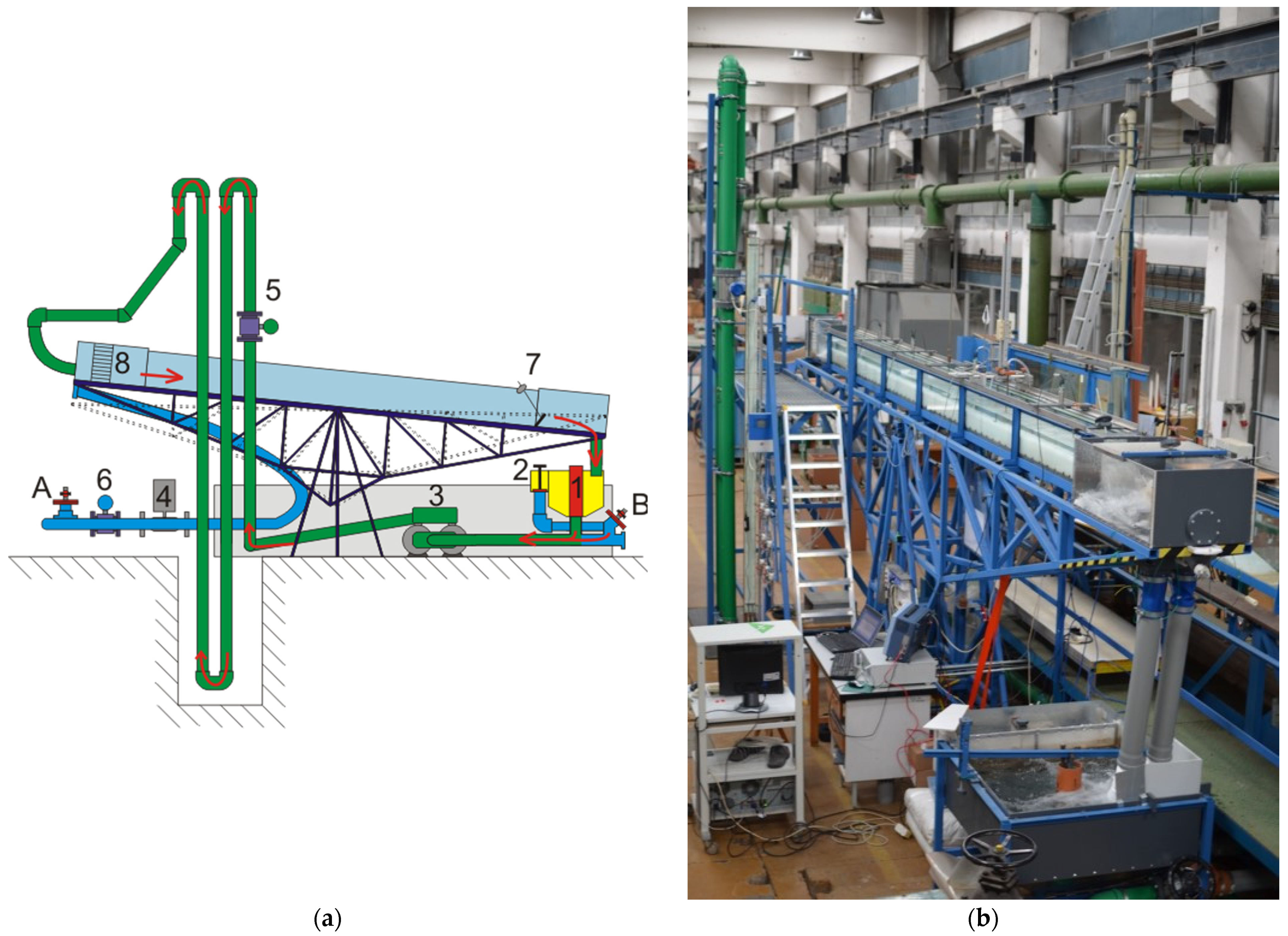
Experiments for calibration and validation of the combined-load model were carried out in a recirculating titling flume (Figure 2) at Water Engineering Laboratory of Czech Technical University in Prague. The set-up was used in several recently reported sediment-transport experiments and it was described in detail elsewhere [24,26]. The flume is 6-m long, 0.2-m wide and allows for various longitudinal slopes including steep ones. In a typical sediment-transport test, an appropriate combination of the longitudinal slope and the mixture flow rate is installed to set required flow conditions for an experimental observation. The mixture flow rate is controlled by the speed of a centrifugal pump (No. 3 in Figure 2) equipped with a variable frequency drive.
2.2.2. Measuring Techniques
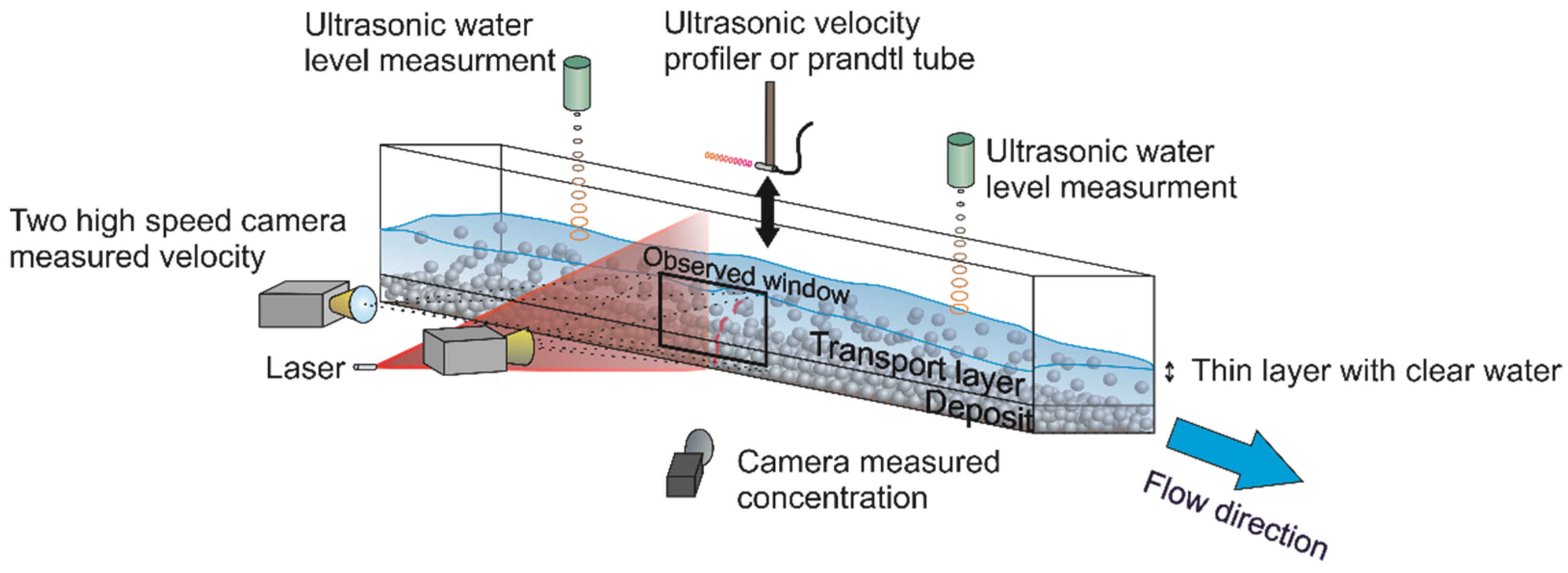
The measuring techniques include a magnetic flow meter (No. 5 in Figure 2) for mixture flow rate, the set of two differential pressure transmitters for the mixture density (DPTs are installed in the vertical pipes of the circuit) and a set of ultrasonic water level sensors along the length of the flume to check the uniformity of mixture flow in the flume and to determine the flow depth depending on the thickness of the sediment bed at the bottom of the flume. In a measuring cross section perpendicular to the flow, distributions are measured of flow velocity and sediment concentration between the top of the sediment bed and the water surface.
In the experiments reported here, the distribution of sediment velocities above the bed was measured by the stereoscopic method using a set of two high-speed cameras (Figure 3). The method and the equipment are described in [26]. In some tests, the longitudinal velocity of sediment particles was also measured at various elevations in the flow cross section by the horizontal-oriented UVP sensor (the technique and method described in [24,33]). Longitudinal velocities of fluid were measured along the flow depth by a Prandtl tube [24]. The distribution of volumetric concentration of transported particles across the flow depth was measured by the laser stripe technique using a camera and a stripe-producing laser (Figure 3) [12,26,34].
2.2.3. Tested Solids
Flow of mixture of water and lightweight sediment above a plane bed composed of the same sediment was tested in the flume. The sediment was a fraction of plastic and virtually mono-size particles (fraction code SUN25) of an approximately prismatic shape (red particles in Figure 1). The experimentally determined properties of the tested solids are summarized in Table 1.
2.2.4. Experimental Flow Conditions
Tests were carried out for flow conditions which ensured a plane surface of the erodible bed, intense transport of sediment and combined load regime. Basically, the first two conditions were controlled by a value the bed Shields parameter, while the last condition required to stay within a certain range of values of the suspension ratio as suggested in [8]. These requirements, together with operability limits of the measuring set-up, constrained ranges of flow quantities attainable in the tests. Nevertheless, a sufficiently broad range of conditions was reached and included the conditions very near the limits of the combined-load regime. In the entire data set, the longitudinal slope varied between 0.25 deg and 2.04 deg and the mixture flow rate between 5.1 L/s and 12.0 L/s. The resulting flow depth varied from 42 mm to 83 mm and the bed Shields parameter from 0.45 to 2.0.
2.2.5. Experimental Data Set
Two experimental campaigns were carried out. The first campaign provided experimental data at different longitudinal slopes and flow depths to cover flow conditions in a sufficiently broad range of the bed Shields parameter to calibrate some of the model constants. The tests included measurements of velocity distributions using three independent techniques (camera, UVP, Prandtl tube) and measurements of concentration profiles using the laser-stripe method. Later, a validation test campaign was executed with the same sediment at slightly different flow conditions, primarily at bigger flow depths and mixture flow rates and milder longitudinal slopes than in the calibration campaign. The conditions captured as broad as possible range of values of bed Shields parameter including those near the limits of the upper plane bed regime. The validation tests did not include UVP measurements due to time constraints. However, the calibration tests confirmed a previously observed good agreement among results of all three methods in the particle rich parts of the flow (the combined-load layer and the lower part of the suspended-load layer) and thus the absence of UVP data in the validation data set did not pose a problem for model validation. Selected results of the validation tests are discussed below.
3. Results
3.1. Experimental Results
In the following, results of selected validation test runs are summarized and discussed. The selection covers a wide range of bed shear conditions from those at the maximum Shields parameter attainable in the experiments to those at so low value of the Shields parameter that the presence of suspended load in the transported sediment is negligible (the suspension ratio of the bed shear velocity and the terminal settling velocity w is significantly lower than 1). Table 2 summarizes experimental conditions for five selected test runs from the validation data set. In Table 2, θ0,flow is obtained from the measured H and ω using Equation (17) and u*0,flow is based on θ0,flow.
3.1.1. Concentration Profiles
The measured shapes of concentration profiles exhibit systematic local changes in trends which indicate an existence of the layered structure of the tested flow and suggest positions of the layer interfaces (the right-hand-side panels in Figure 4). In the lowest part of a profile, there is a characteristic sharp change in the concentration gradient which becomes considerably steeper at elevations where the local concentration c drops below say 0.45. While the resolution of the measurement is not sufficient to unambiguously detect the elevation and the associated value of the local concentration at which the change actually occurs, it can be hypothesized that the change in the concentration gradient is associated with the change between the predominantly permanent contact regime and predominantly collisional regime of particle interaction in the flow. In the model, this change is associated with the interface between the combined-load layer and the permanent-contact layer. The observed region of the approximately linear profile above the assumed top of the permanent-contact layer justifies the model assumption of a linear profile in the combined-load layer.
Another systematic and detectable feature of the measured concentration profiles is that the profiles can be no longer considered linear at elevations with c lower than say 0.25. This is different from concentration profiles in purely collisional flows, which can be approximated by a line from the bottom to the top of the transport layer [3,26]. Therefore, the non-linear shape of the profile can be attributed to the dominating turbulent suspension of particles and the lower boundary of the non-linear profile can be considered the interface between the combined-load layer and the suspended-load layer. The region occupied by the non-linear profile is the largest in the flow with the highest value of u*0,flow/w (Test 1: u*0,flow/w = 1.57, see Table 2) where it spans a distance between the assumed top of a thin combined-load layer and some position very near the water surface, i.e., the interval 5 < y < 20 approximately (Figure 4). If the u*0,flow/w value decreases (Tests 2 to 5), then the region of full suspension narrows, its top departs from the water surface and leaves an increasingly thick particle-free zone below the water surface. At the lowest u*0,flow/w (equal to 0.86 in Test 5), the full-suspension region is marginal and can be neglected. Note also that the permanent-contact layer tends to become thinner if the applied bed shear stress (the bed Shields parameter) decreases. In general, this layer is considerably thinner than the other layers at all bed shear conditions covered by Tests 1–5.
3.1.2. Velocity Profiles
The velocity profiles measured in Tests 1–5 all exhibit a region of an approximately linear profile which corresponds with the region delimited by the boundaries of the combined-load layer and which exhibits also a linear concentration profile (the left-hand-side panels of Figure 4). In this region, there is a very good agreement between local velocities measured by two different measuring techniques: The Prandtl tube (sensing local fluid velocity) and the stereoscopic technique (sensing local solids velocity). It indicates that a difference in local velocities of fluid and particles can be neglected. Additional measurements of the sediment velocity by UVP used in the calibration tests confirmed a good accuracy of the stereoscopic method and this was consistent with our previous observations for different lightweight sediment in the flume [26]. However, the agreement between results from the Prandtl tube and from the stereoscopic method is considerably weaker in the particle-lean region above the top of the linear profile (i.e., in the suspended-load layer) where a measured velocity profile is no longer linear. The local velocities by the stereoscopic method are systematically lower than those by the Prandtl tube and the difference seems to increase with the decreasing local concentration of sediment at positions closer to the water surface. It can be attributed to lower accuracy of the stereoscopic method in a flow domain with a low population of particles. The observed deviation is again consistent with our previous observations [26].
3.2. Model Predictions
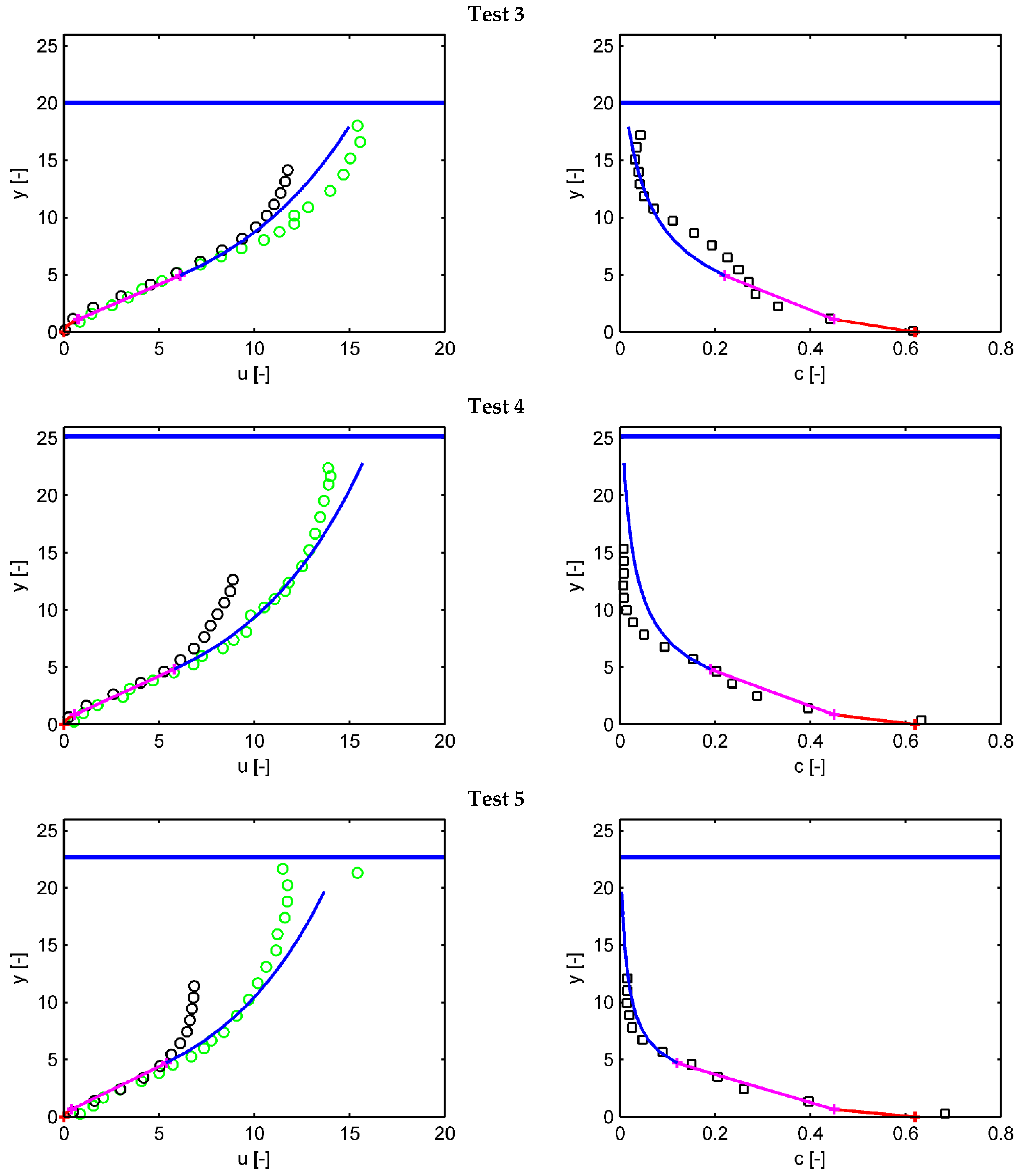
Distributions of concentration and velocity are predicted by the model for the conditions of Tests 1–5 (see Table 2) following the procedure described in Section 2.1.5. The predictions include the elevations of interfaces in the sediment-water flow and they are presented in Figure 4 together with the experimentally determined distributions. Parts of the predicted profiles of velocity and concentrations are plotted in different colors to distinguish among predicted layers across the flow depth.
In the model calculations, the effective coefficient of restitution in dry conditions ε = 0.60 and the particulate friction coefficient β0 = 0.65 are employed for the SUN25 sediment.
3.2.1. Concentration Profiles
Based on the model assumptions, the predicted distributions of solids are linear across the permanent-contact layer and the combined-load layer. The slopes of the profiles result from the predicted elevations of the layer interfaces (yd, yc) above the bed (y0 = 0), from the chosen values of the local concentrations at the interfaces (c0, cd) and from the calculated cc at yc. The values of c0 = ccr (ccr = 0.62) and cd = 0.45 were chosen for all test runs to be consistent with the measured values of c at the positions of the abrupt change in a concentration gradient as discussed above. At the d-boundary, cd was considered the freeze concentration (cd = cf) to satisfy the kinetic-theory based condition for dense limit (Ld = 1). The cf is sensitive to the shape of particles and this justifies its chosen value which is slightly lower for our tested particles than for particles of simple shapes (e.g., 0.49 for cylindrical particles). In the suspended-load layer, a predicted shape of the concentration profile is sensitive to the particle diffusivity constant, Cη = 2 was used for all tested flow conditions.
3.2.2. Velocity Profiles
The model assumptions for velocity gradients define shapes of velocity profiles in the permanent-contact layer (the shear rate γ linearly distributed) and in the combined-load layer (the shear rate constant). The shear rate is assumed equal to zero at the bed (γ0 = 0) and it is calculated by a constitutive relation at the d-boundary (Equation (7)). At the c-boundary, γc = γd. The predicted elevations yd and yc determine ud and uc. In the suspended-load layer, a predicted shape of the velocity profile is logarithmic and affected by the local mixing length (κ = 0.41) and by the initial position determined empirically using the constant Cini, which is the same for all tested flow conditions (Cini = 1.65).
4. Discussion
Comparisons of the predicted and measured distributions of velocity and concentration show very reasonable agreement and indicate that the model is capable of capturing the layered character of the flow with intense transport of combined load (Figure 4). The distributions inside the individual layers are captured well too, although more detailed modelling of processes at the local level may provide more precise information about the distributions, particularly in the suspended load layer. If the suspended-load layer is thick (Tests 1 to 3 in Figure 4), it tends to exhibit a complex shape of the concentration profile composed of a convex part and a concave part. This change in the profile shape in the central region of the layer cannot be reproduced by the current model.
The transport model has been calibrated and validated by results of our own experiments which produced sufficiently detailed information about the tested flows including information on the local level from the channel bed to the water surface. Those experimental results are quite unique and enabled to test model abilities in a broad range of conditions including those close to the limits of combined-load transport.
A prediction of distributions of velocity and concentration provides information that enables to determine flow rates of mixture and its phases for the modelled flow. It makes the model a useful tool from an engineering perspective as it is capable of simulating mutual relations among the longitudinal slope, the flow depth, the flow rate of sediment and the total flow rate of sediment-water mixture. In this sense, the model is a more physically sound alternative to currently widely used empirical transport models.
Note also that the proposed transport model does not require the bed friction law which the above-mentioned empirical transport models need. In such models, the friction formula for the top of the erodible bed interacting with particles transported above the bed is a significant source of uncertainty affecting a determination of the relation between the flow rate, the flow depth and the water surface elevation. The uncertainty is associated primarily with difficulties in the interpretation of the roughness of the erodible bed at the condition of intense transport of sediment above the bed. This problem is avoided in the proposed model and hence it solves the bed friction problem in a more elegant way.
However, future work is required to further refine the model. Modelling of the quite specific conditions at the bottom of the combined-load layer, which seem to differ from conditions at the bottom of a purely collisional layer and which are therefore more challenging to describe using the kinetic-theory based constitutive relations, must be addressed so that the reduction constant Cbd can be removed. Furthermore, modelling of interactions of suspended particles with turbulent flow in the sediment-rich region just above the top of the combined-load layer requires a refinement to reproduce more closely the characteristic shape of a concentration profile observed experimentally in this region.
Funding
This research was funded by Czech Science Foundation, grant number 19-18411S.
Data Availability Statement
The data presented in this study can be found here: https://www.researchgate.net/publication/358553772_data_SUN25_Tests_1-5_article_Water_2022 (accessed on 21 December 2021).
Conflicts of Interest
The author declares no conflict of interest.
Abbreviations
| ACVP | Acoustic Concentration and Velocity Profiler |
| DPT | Differential Pressure Transmitter |
| ERT | Electrical Resistivity Tomography |
| UVP | Ultrasonic Velocity Profiler |
Appendix A
Conversion between dimensionless and dimensional quantities
length:
density:
velocity:
velocity gradient:
granular temperature:
stress:
fluid dynamic viscosity:
References
- Cao, Z.; Pender, G.; Meng, J. Explicit formulation of the Shields diagram for incipient motion of sediment. J. Hydraul. Eng. 2006, 132, 1097–1684. [Google Scholar] [CrossRef]
- Garcia, M.M. Sedimentation Engineering; American Society of Civil Engineers: Reston, VA, USA, 2008. [Google Scholar]
- Capart, H.; Fraccarollo, L. Transport layer structure in intense bed-load. Geophys. Res. Lett. 2011, 38, L20402. [Google Scholar] [CrossRef]
- Revil-Baudard, T.; Chauchat, J.; Hurther, D.; Barraud, P.-A. Investigation of sheet-flow processes based on novel acoustic high-resolution velocity and concentration measurements. J. Fluid Mech. 2015, 767, 1–30. [Google Scholar] [CrossRef] [Green Version]
- Pugh, F.J.; Wilson, K.C. Velocity and concentration distributions in sheet flow above plane beds. J. Hydraul. Eng. 1999, 125, 117–125. [Google Scholar] [CrossRef]
- Matoušek, V. Concentration profiles and solids transport above stationary deposit in enclosed conduit. J. Hydraul. Eng. ASCE 2009, 135, 1101–1106. [Google Scholar] [CrossRef]
- Gillies, R.G.; Shook, C.A. Concentration distributions of sand slurries in horizontal pipe flow. Part. Sci. Technol. 1994, 12, 45–69. [Google Scholar] [CrossRef]
- Sumer, B.M.; Kozakiewitz, A.; Fredsøe, J.; Deigaard, R. Velocity and concentration profiles in sheet-flow layer of movable bed. J. Hydraul. Eng. 1996, 122, 549–558. [Google Scholar] [CrossRef]
- Matoušek, V.; Krupička, J.; Picek, T. Validation of transport and friction formulae for upper plane bed by experiments in rectangular pipes. J. Hydrol. Hydromech. 2013, 61, 120–125. [Google Scholar] [CrossRef] [Green Version]
- Capart, H.; Young, D.L.; Zech, Y. Voronoi imaging methods for the measurement of granular flows. Exp. Fluids 2002, 32, 121–135. [Google Scholar] [CrossRef]
- Spinewine, B.; Capart, H.; Larcher, M.; Zech, Y. Three-dimensional Voronoi imaging methods for the measurement of near-wall particulate flows. Exp. Fluids 2003, 34, 227–241. [Google Scholar] [CrossRef]
- Spinewine, B.; Capart, H.; Fraccarollo, L.; Larcher, M. Laser stripe measurements of near-wall solid fraction in channel flows of liquid-granular mixtures. Exp. Fluids 2011, 50, 1507–1525. [Google Scholar] [CrossRef]
- Armanini, A.; Capart, H.; Fraccarollo, L.; Larcher, M. Rheological stratification in experimental free-surface flows of granular-liquid mixtures. J. Fluid Mech. 2005, 532, 269–319. [Google Scholar] [CrossRef] [Green Version]
- Larcher, M.; Fraccarollo, L.; Armanini, A.; Capart, H. Set of measurement data from flume experiments on steady uniform debris flows. J. Hydraul. Res. 2007, 45, 59–71. [Google Scholar] [CrossRef]
- Spinewine, B.; Capart, H. Intense bed-load due to a sudden dam-break. J. Fluid Mech. 2013, 731, 579–614. [Google Scholar] [CrossRef]
- Cheng, Z.; Hsu, T.-J.; Calantoni, J. Sedfoam: A multi-dimensional Eulerian two-phase model for sediment transport and its application to momentary bed failure. Coast. Eng. 2017, 119, 32–50. [Google Scholar] [CrossRef] [Green Version]
- Gonzalez-Ondina, J.M.; Fraccarollo, L.; Liu, P.L.F. Two-level, two-phase model for intense, turbulent sediment transport. J. Fluid Mech. 2018, 839, 198–238. [Google Scholar] [CrossRef] [Green Version]
- Berzi, D. Analytical solution of collisional sheet flows. ASCE J. Hydraul. Eng. 2011, 137, 1200–1207. [Google Scholar] [CrossRef]
- Berzi, D.; Fraccarollo, L. Inclined, collisional sediment transport. Phys. Fluids 2013, 25, 106601. [Google Scholar] [CrossRef] [Green Version]
- McTigue, D.F. Mixture theory for suspended sediment transport. J. Hydraul. Div. ASCE 1981, 107, 659–673. [Google Scholar] [CrossRef]
- Wilson, K.C.; Pugh, F.J. Dispersive-force modelling of turbulent suspension in heterogeneous slurry flow. Can. J. Chem. Eng. 1988, 66, 721–727. [Google Scholar] [CrossRef]
- Berzi, D. Transport formula for collisional sheet flows with turbulent suspension. J. Hydraul. Eng. 2013, 139, 359–363. [Google Scholar] [CrossRef]
- Berzi, D.; Fraccarollo, L. Intense sediment transport: Collisional to turbulent suspension. Phys. Fluids 2016, 28, 023302. [Google Scholar] [CrossRef] [Green Version]
- Matoušek, V.; Bareš, V.; Krupička, J.; Picek, T.; Zrostlík, Š. Experimental investigation of internal structure of open-channel flow with intense transport of sediment. J. Hydrol. Hydromech. 2015, 63, 318–326. [Google Scholar] [CrossRef] [Green Version]
- Matoušek, V.; Zrostlík, Š. Laboratory testing of granular kinetic theory for intense bed load transport. J. Hydrol. Hydromech. 2018, 66, 330–336. [Google Scholar] [CrossRef]
- Matoušek, V.; Zrostlík, Š.; Fraccarollo, L.; Prati, A.; Larcher, M. Internal structure of intense collisional bed load transport. Earth Surf. Process. Landf. 2019, 44, 2285–2296. [Google Scholar] [CrossRef]
- Matoušek, V.; Zrostlík, Š. Collisional transport model for intense bed load. J. Hydrol. Hydromech. 2020, 68, 60–69. [Google Scholar] [CrossRef] [Green Version]
- Matoušek, V.; Zrostlík, Š. Combined load in open channel: Modelling of transport layer at high bed shear. In Proceedings of the River Flow 2020, Delft, The Netherlands, 7–10 July 2020; Uijttewaal, W., Franca, M.J., Valero, D., Chavarrias, V., Arbós, C.Y., Schielen, R., Crosato, A., Eds.; Taylor & Francis Group: London, UK, 2020; pp. 308–315. [Google Scholar]
- Berzi, D.; Fraccarollo, L. Turbulence locality and granularlike fluid shear viscosity in collisional suspensions. Phys. Rev. Lett. 2015, 115, 194501. [Google Scholar] [CrossRef] [Green Version]
- Berzi, D.; Larcan, E. Flow resistance of inertial debris flows. J. Hydraul. Eng. 2013, 139, 187–194. [Google Scholar] [CrossRef]
- Garzó, V.; Dufty, J.W. Dense fluid transport for inelastic hard spheres. Phys. Rev. E 1999, 59, 5895. [Google Scholar] [CrossRef] [Green Version]
- Torquato, S. Nearest-neighbor statistics for packings of hard spheres and disks. Phys. Rev. E 1995, 51, 3170–3182. [Google Scholar] [CrossRef]
- Bareš, V.; Zrostlík, Š.; Picek, T.; Krupička, J.; Matoušek, V. On local velocity measurement in gravity-driven flows with intense bedload of coarse lightweight particles. Flow Meas. Instrum. 2016, 51, 68–78. [Google Scholar] [CrossRef]
- Krupička, J.; Picek, T.; Zrostlík, Š. Reduction of uncertainties in laser stripe measurement of solid particles concentration. Acta Polytech. 2018, 58, 171–178. [Google Scholar] [CrossRef]
Figure 1.
Layered structure of modelled flow including schematic concentration profile projected onto photograph of combined-load transport in tilting flume.
Figure 1.
Layered structure of modelled flow including schematic concentration profile projected onto photograph of combined-load transport in tilting flume.

Figure 2.
Experimental set-up in Water Engineering Laboratory: (a) Lay-out of the recirculating system with tilting flume; (b) Overall view of recirculating system [26].
Figure 2.
Experimental set-up in Water Engineering Laboratory: (a) Lay-out of the recirculating system with tilting flume; (b) Overall view of recirculating system [26].

Figure 3.
Schematic layout of tilting flume and measuring equipment in Water Engineering Laboratory [26].
Figure 3.
Schematic layout of tilting flume and measuring equipment in Water Engineering Laboratory [26].

Figure 4.
Profiles of velocity (left panels) and concentration (right panels) in Tests 1–5 for flow with transported SUN25 particles in tilting flume (all quantities are dimensionless). Legend: Black circle—stereoscopic measurement; green circle—Prandtl tube measurement; black square—laser-stripe measurement; red line—model prediction in permanent-contact layer; magenta line—prediction in combined-load layer; blue line—prediction in suspended-load layer; horizontal blue line—water surface.


Table 1.
Properties of tested solids: Particle equivalent diameter d, specific gravity S, terminal settling velocity w, particle Reynolds number R.
Table 1.
Properties of tested solids: Particle equivalent diameter d, specific gravity S, terminal settling velocity w, particle Reynolds number R.
| SUN25 | |
|---|---|
| d [mm] | 2.8 |
| S [-] | 1.28 |
| w [mm/s] | 76.5 |
| w [-] | 0.987 |
| R [-] | 217 |
Table 2.
Combined-load experiment in tilting flume: Experimental conditions for Tests 1 to 5 (longitudinal slope ω, flow depth H, flow Reynolds number Re, bed Shields parameter θ0,flow, suspension ratio u*0,flow/w; all quantities are dimensionless).
Table 2.
Combined-load experiment in tilting flume: Experimental conditions for Tests 1 to 5 (longitudinal slope ω, flow depth H, flow Reynolds number Re, bed Shields parameter θ0,flow, suspension ratio u*0,flow/w; all quantities are dimensionless).
| Test 1 | Test 2 | Test 3 | Test 4 | Test 5 | |
|---|---|---|---|---|---|
| ω [-] | 0.0257 | 0.0142 | 0.0154 | 0.0098 | 0.0070 |
| H [-] | 20.4 | 25.5 | 20.0 | 25.1 | 22.7 |
| Re [-] | 4.0 × 10⁴ | 6.1 × 10⁴ | 4.1 × 10⁴ | 5.1 × 10⁴ | 4.0 × 10⁴ |
| θ0,flow [-] | 1.88 | 1.30 | 1.10 | 0.88 | 0.57 |
| u*0,flow/w [-] | 1.57 | 1.31 | 1.20 | 1.08 | 0.86 |
Publisher’s Note: MDPI stays neutral with regard to jurisdictional claims in published maps and institutional affiliations. |
© 2022 by the author. Licensee MDPI, Basel, Switzerland. This article is an open access article distributed under the terms and conditions of the Creative Commons Attribution (CC BY) license (https://creativecommons.org/licenses/by/4.0/).
Share and Cite
MDPI and ACS Style
Matoušek, V. Modelling Intense Combined Load Transport in Open Channel. Water 2022, 14, 572. https://doi.org/10.3390/w14040572
AMA Style
Matoušek V. Modelling Intense Combined Load Transport in Open Channel. Water. 2022; 14(4):572. https://doi.org/10.3390/w14040572
Chicago/Turabian StyleMatoušek, Václav. 2022. "Modelling Intense Combined Load Transport in Open Channel" Water 14, no. 4: 572. https://doi.org/10.3390/w14040572
Note that from the first issue of 2016, this journal uses article numbers instead of page numbers. See further details here.