
Short-Term Hydrological Forecast Using Artificial Neural Network Models with Different Combinations and Spatial Representations of Hydrometeorological Inputs

Département de Génie Civil et de Génie du Bâtiment, Université de Sherbrooke, Sherbrooke, QC J1K 2R1, Canada
*
Author to whom correspondence should be addressed.
Water 2022, 14(4), 552; https://doi.org/10.3390/w14040552
Submission received: 19 January 2022
/
Revised: 9 February 2022
/
Accepted: 10 February 2022
/
Published: 12 February 2022
(This article belongs to the Topic Recent Advances in Hydroinformatics: Focusing on Machine Learning and Remote Sensing in Hydrology)
Abstract
:In hydrological modelling, artificial neural network (ANN) models have been popular in the scientific community for at least two decades. The current paper focuses on short-term streamflow forecasting, 1 to 7 days ahead, using an ANN model in two northeastern American watersheds, the Androscoggin and Susquehanna. A virtual modelling environment is implemented, where data used to train and validate the ANN model were generated using a deterministic distributed model over 16 summers (2000–2015). To examine how input variables affect forecast accuracy, we compared streamflow forecasts from the ANN model using four different sets of inputs characterizing the watershed state—surface soil moisture, deep soil moisture, observed streamflow the day before the forecast, and surface soil moisture along with antecedent observed streamflow. We found that the best choice of inputs consists of combining surface soil moisture with observed streamflow for the two watersheds under study. Moreover, to examine how the spatial distribution of input variables affects forecast accuracy, we compared streamflow forecasts from the ANN using surface soil moisture at three spatial distributions—global, fully distributed, and single pixel-based—for the Androscoggin watershed. We show that model performance was similar for both the global and fully distributed representation of soil moisture; however, both models surpass the single pixel-based models. Future work includes evaluating the developed ANN model with real observations, quantified in situ or remotely sensed.
1. Introduction
Among natural disasters, hydrological-related damage has the greatest impact on humanity and its activities [1]. Major events can be either floods or droughts. According to the United Nations, 2437 million people were affected by floods from 1992 to 2012, with an estimated cost of 480 USD billion [2]. In northern regions, floods are typically caused by: (i) snowmelt in the spring, which can be compounded by ice jams and/or rainfall, and (ii) high rainfall due to severe thunderstorms or very active low-pressure systems during the summer and fall. More specifically in the northeastern part of North America, large rainfalls events are associated with the tail of hurricanes, originating from the Atlantic Ocean and reaching the Caribbean and the Gulf of Mexico. In this context, flood forecasting agencies and research centers are developing and improving hydrological models and forecasting systems to anticipate floods and mitigate their impacts [3,4,5]. Hydropower companies are also involved in model development and contribute to knowledge in hydrological modelling.
Central to a hydro-meteorological forecasting chain is the hydrological model. To date, conceptual and physically based deterministic hydrological models have typically been used by flood forecasting agencies; for example, HYDROTEL [3] at the Direction de l’Expertise Hydrique et de l’Atmosphère (DEHA, in English: Center for Water and Atmosphere Expertise) of Québec (Canada); Distributed Hydrological-Soil-Vegetation Model [6] at the Advanced Hydrologic Prediction Services, associated with the National Oceanographic and Atmospheric Administration in the USA; Weather Research and Forecasting produced by Hydro at River Forecast Centers across the USA; and MODCOU [7] at the Service Central d’Hydrométéorologie et d’Appui à la Prévision des Inondations (in English: Hydrometeorological and Flood Forecasting Central Service) in France. They all have several years of applicability and performance in common and are being continuously developed by their respective agencies and affiliated research centers. These agencies and others involved in operational streamflow forecasting face four main challenges, described by [8] as follows: “(1) making the most of available data, (2) making accurate predictions using models, (3) turning hydrometeorological forecasts into effective warnings, and (4) administering an operational service” ([8], p. 1692). The authors highlight several weaknesses of current models, among which are the high computational resources and the difficulty in simulating fine spatial resolution hydrological processes. While they propose some opportunities to improve the streamflow forecasting chain, data-driven models present a high potential to answer some of these issues [9].
One type of data-driven model is machine learning (ML), commonly defined as a process in which a computer learns from a historical dataset and then makes predictions. ML models can be used across a wide range of applications such as finance, marketing, medicine, and hydrology, among others and advantages include the efficiency in handling multi-dimensional data and complex environments, improving accuracy and successful over time, and reducing costs [10,11]. However, some limitations should be noted, in particular the need for a large amount of geomorphological and hydrometeorological data and the poor efficiency in transfer learning. A wide range of ML models are available and found in the literature [10,12,13]. To the best of the authors’ knowledge, and although ML models in hydrology have been investigated by the scientific community, such models used operationally by companies or public services to produce flood forecasts are still scarce. GeoSapiens, FlowWorks, and UpstreamTech are three North American companies that illustrate the use of ML in a direct operational application in hydrology—specifically, in flood risk-reduction systems. Several articles have compared the performance of traditional deterministic models versus ML models; however, there is no clear consensus for which approach is better for hydrological modelling. [14,15,16] are three good examples of testing artificial neural networks (ANNs) for flood forecasting. ANN models are a popular ML approach for hydrological modelling and forecasting [17]. Several papers have demonstrated hydrological applications of ANN models, mostly for forecasts issued a few hours up to a season in advance [17,18,19,20]. Typical of ML models, ANN is efficient in resolving non-linear problems. However, compared to other ML approaches, the primary advantage of ANN models is their capacity to learn continuously—their internal structure allows the model to update the learning process at each timestep without a high cost in time and resources. Moreover, compared to physically based hydrological models, using ANN models operationally does not require extensive hydrological expertise; flood forecasting agencies that use physically based models usually host specific teams devoted to the various tasks involved in a traditional hydro-meteorological forecasting chain. For example, running a physically based hydrological model requires human checks and decisions at each step, from the inputs to the internal parameters of the model to the outputs. Such tasks require considerable resources, including updating and maintaining physiographic and hydrometeorological databases that are needed to calibrate and run models. The three national agencies cited above are good examples of the wealth of expertise needed to issue accurate hydrological forecasts from physically based models. The procedure should be largely reduced with ANN models. The main issue that arises using ANN models is overfitting the model to the training data. Another challenge is the low convergence of models during the learning step with some structures of ANN models [1,21].
In ML hydrological modelling, including via ANN models, clear identification of the inputs and output(s) is necessary. Inputs are a key element to train an efficient model [22] and are likely to differ according to the forecasting horizon. For long-term forecasts (i.e., several months or seasons in advance), variables describing climatic trends are most commonly used as inputs. In contrast, for short-term forecasts (i.e., from 1 h to a few days in advance), inputs should be variables that have a rapid effect on the hydrological processes of interest. These are generally variables that are measured at discrete locations using ground probes (e.g., temperature, precipitation, and snow depth), but also can be quantified across large spatial extents using remote sensing (e.g., soil moisture, snow water equivalent, and precipitation). At least one watershed state variable—variables describing water stored by the watershed (e.g., streamflow the day before), soil (e.g., soil moisture), or land surface (e.g., snow depth and/or snow water equivalent)—should be included as inputs. Hydrological watershed behavior is directly related to streamflow, therefore streamflow provides information on water storage across the entire watershed. Soil moisture is particularly relevant to forecasts in summer and fall because it plays an important role in runoff and infiltration, while snow is relevant in winter and spring forecasts as it contains information about the water stored during the frozen season. Users should select one or more of these watershed state variables depending on model intended use (e.g., spring or summer/fall flood events) and on the availability of information describing watershed state variables. For short-term hydrological forecasts, model outputs are commonly streamflow [9,23,24], runoff [25], or water level [26].
Regardless of the type of model implemented (i.e., conceptual, physically-based, or ML approaches), decisions surrounding how watershed heterogeneity is represented need to be made; primarily dependent on the dominant hydrological process being modeled or forecasted. Global models, such as the family of GR models [27,28], consider the watershed as a single unit whereas, semi-distributed models divide the watershed into hydrological units that are considered homogeneous; for example, relative homogeneous hydrological units (RHHU) in HYDROTEL [3] and hydrological response units (HRU) in the Soil and Water Assessment Tool model [29]. Finally, fully distributed models subdivide the watershed into a grid, which is usually regular, such as TOPMODEL [30] and WRF-Hydro [5]. Refs. [31,32] highlight that there is not a clear advantage in using one spatial distribution over another. For ML modelling, the user should decide on the spatial distribution of the model based on the available data and the application the model will be used for. For example, [33] applied a fully distributed model to predict water level where ANN inputs were remotely sensed, satellite-gridded data from CHIRPS, GLDAS-2, and TRMM-V7.
In this study, we investigate different means to represent the watershed hydrological state in an ANN model used for short-term hydrological forecasts related to runoff events triggered by rainfall alone. Specifically, we first aimed to understand how current soil moisture at different depths and streamflow affect short-term streamflow forecasts by assessing the performance of an ANN rainfall-runoff model using different combinations of hydrometeorological inputs. Then, we examined how global and spatialized inputs affect ANN model performance. To do so, we generated a virtual hydrological environment with a semi-distributed hydrological model simulating watershed state variables and the hydrological response of two real watersheds under real meteorological forcings. The simulated hydrometeorological observations (i.e., outputs from the semi-distributed hydrological model) were then used as inputs—using different combinations and spatial configurations—to the ANN model. We found that hydrological forecasts are better across a 7-day forecast window when combining streamflow and soil moisture as watershed state variables inputs instead compared to forecasts made using them separately as inputs. Moreover, we found that considering the spatial heterogeneity of soil moisture improved forecasting compared to a global model.
2. Materials and Methods
2.1. Study Area
This study was conducted using two watersheds in the northeastern United States: the Susquehanna watershed, mainly in New York and Pennsylvania, and the Androscoggin watershed, primarily located in Maine (Figure 1). The Susquehanna watershed is the larger of the two, with an area of 71,225 km2. The Susquehanna River is the longest in the New England region, originating in the Allegheny Plateau and draining into the Chesapeake Bay on the Atlantic Ocean. The Susquehanna River is relatively flat, spanning approximately 360 m in elevation, with its maximum elevation at the Ostego Lake headwater located in the northeast of the watershed. Land use across the Susquehanna watershed is diverse, where 59% of the watershed area is forested, 31.5% is agricultural lands, 6.5% is rocks and urbanized areas, and 3% is wetlands. In contrast, the Androscoggin watershed is relatively small, with an area of 8935 km2. The Androscoggin River has comparatively elevation, spanning approximately 379 m in elevation, with its maximum elevation located along the western border of the watershed. The Androscoggin River drains into Merrymeeting Bay on the Atlantic Ocean. The Androscoggin watershed is primarily forested, with forests covering 83.5% of the watershed area. Other land covers are wetlands, rocks, and urbanized soils, and agricultural lands representing 8.5%, 8.5%, and 3.5% of the total watershed area, respectively. The United States Geological Survey (USGS) has streamflow stations located close to the outlets of both watersheds (as indicated by the red triangles in Figure 1).
The climatic and hydrological regimes of both watersheds are typical of northern watersheds. Heavy spring floods are the result of large volumes of meltwater following cold and snowy winters, while summer and fall floods are mainly the results of heavy precipitation and storms. Typical of medium to large watersheds in northern latitudes, the spring flood is more significant than the summer and fall floods for both watersheds—as visually evident in the mean annual streamflow hydrographs derived from the USGS streamflow stations (Figure 2). The size of each watershed largely explains the differences in streamflow (Table 1), where the Susquehanna watershed is about eight times bigger than the Androscoggin watershed and has a maximum streamflow of 2828 m3/s compared to Androscoggin’s maximum streamflow of 516 m3/s.
2.2. Hydrometeorological Inputs
We conducted this study in a virtual hydrological environment. Consequently, the time-series data sets used as ANN inputs do not contain any missing data or outliers and have a similar level of confidence. Inputs to the ANN model were derived from HYDROTEL, a deterministic model [3], as described below.
We chose to use HYDROTEL to generate ANN inputs for two main reasons, (i) HYDROTEL is a semi-distributed model and, therefore, allows us to explore the possibilities of how spatial discretization of model inputs affects ANN model performance and (ii) the simulation option BV3C (Bilan Vertical à 3 Couches, in English: Three-Layer Vertical Budget) within HYDROTEL, presented below, models the vertical water budget and thus allows us to incorporate soil moisture ‘observations’ at various depths as input to the ANN.
HYDROTEL is a semi-distributed hydrological model that simulates a large set of hydrological processes across discrete spatial units, called RHHU, which collectively represent the watershed of interest. RHHUs are characterized as areas with relatively homogeneous land cover and soil properties that are drained by one river segment, or reach. PHYSITEL uses different layers of physiographic information, including: soil type, land cover, and topography, to first determine the drainage network of watersheds and subsequently discretize watersheds into RHHUs [3]. Using PHYSITEL, we defined 1025 and 403 RHHUs for the Susquehanna and Androscoggin watersheds, respectively.
HYDROTEL has six internal sub-models that offer different simulation options (Table 2). Requiring only three meteorological inputs (precipitation, minimum temperature, and maximum temperature), HYDROTEL simulates 23 outputs at a daily timestep and across all RHHUs (outputs include: snow, soil moisture at different soil depths, evapotranspiration, inflow, etc.) or river reaches (outputs include: upstream and downstream streamflow). For each sub-model, we chose one simulation option to generate hydrometeorological observations (i.e., the HYDROTEL outputs) that were subsequently used as inputs to the ANN model for both the Susquehanna and Androscoggin watersheds (Table 2; the selected simulation options are bolded). One of our motivations for using HYDROTEL is the simulation option BV3C in the vertical water budget sub-model, as it incorporates infiltration and vertical flows in the soil column (Figure 3). Briefly, BV3C divides the soil column into three layers (Z1, Z2, and Z3 in Figure 3). The first layer represents a thin soil layer at the soil surface that controls infiltration, the second layer is associated with interflow (Q2 in Figure 3), and the third layer simulates base flow (Q3 in Figure 3) [3]. This vertical water budget is computed individually for each RHHU. Soil moisture and evapotranspiration are then available for the three layers (Θ1, Θ2, and Θ3, and ETR1, ETR2, and ETR3, respectively). More details can be found by interested readers on Figure 3 and reading [3].
The Thiessen polygon approach had been selected as the simulation option for the interpolation of precipitation. The watershed area is then divided based on polygons of influence of each precipitation station; any point in a polygon is closer to the station associated to the polygon than any other stations. The modified degree-day simulated snowmelt using temperature and precipitation to approximate energy-budget based on meteorological inputs of the HYDROTEL models and on geomorphological information like slope, surface orientation, and land use. The evapotranspiration is defined with the Hydro-Québec option that is relatively simple, requiring only maximal and minimal temperatures as input. The kinematic wave equation describes how the water runoffs at the surface based on the vertical water budget and UHRH spatial discretization. Finally, the modified kinematic wave equation was used to simulate channel routing. This option permits to consider the geometry of the hydrological reaches (Table 2).
Prior to generating the hydrometeorological ‘observations’, which were used as input data to the ANN, we calibrated HYDROTEL for each watershed using meteorological inputs and observed streamflow data extracted from the USGS database. Model calibration for the Susquehanna and Androscoggin watersheds resulted in soil layer thicknesses of 10 cm, 40 cm, and 50 cm for layers 1, 2, and 3 respectively for Susquehanna; and of 10 cm, 20 cm, and 60 cm for Androscoggin. HYDROTEL was then run over 19 years (1997–2015), including 3 years of warm-up. We selected four HYDROTEL output variables (i.e., the hydrometeorological observations) to be used as input data to the ANNs: total precipitation (solid and liquid), streamflow at the watershed outlet, and soil moisture in the first two layers of soil. Going forward, we refer to the first two layers of soil as either surface soil moisture (i.e., the depth of the first soil layer; 10 cm for both watersheds) or deep soil moisture (i.e., the sum of the depth of the first two layers of soil; top 50 cm and 30 cm for the Susquehanna and Androscoggin, respectively).
It is known that soil moisture [34] and streamflow [35] affect short-term hydrological forecasts. Here the objective is to decipher how ML models can effectively represent this causal relationship. To that end, we ran the ANN model using four different combinations of the hydrometeorological observations as input variables (Table 3). The ANN streamflow forecast was undertaken on a daily timestep over a 7-day window. We classified ANN inputs in two categories: meteorological variables—precipitation taken at the forecast horizon (D) and taken one day before (D-1), and the watershed state variables—antecedent streamflow, surface soil moisture, and deep soil moisture taken 1 day before the forecast horizon (D-1) (Table 3). The meteorological variables represent the incoming water at the forecast day D, while the watershed state variables represent the water already present in the watershed. Here, streamflow is considered as a watershed state variable, although strictly speaking it should be categorized as a flux. To remove the arbitrary effect of similarity between objects [36], including those caused by differences in units between variables, that can confuse ANN models and reduce performance, we normalized the hydrometeorological observation input data before running the ANN model. The normalization process we applied is based on the standardization formula (i.e., subtracting the dataset mean from each element of the dataset and then dividing the difference by the dataset standard deviation).
2.3. Artificial Neural Network (ANN) Model
ANN models are drawn from the operating philosophy of the human brain. This type of model builds on relationships within a data set, connecting inputs (i.e., feature variables) and output(s) (i.e., variable(s) of interest) [19]. ANN models are composed of at least three layers: the input, the hidden, and the output (Figure 4). The input layer introduces the inputs used by the ANN model with one independent node, commonly referred to as a neuron, for each feature variable. Similarly, the output layer is based on one independent node, or neuron, for each variable of interest. The hidden layer establishes relationships between the inputs and outputs, where the number of nodes, or neurons, defines the number of relationships that are prescribed. Depending on the complexity of the problem, more than one hidden layer can be chosen. However, [36] found that multiple hidden layers can always be simplified to a single hidden layer, as long as it has an appropriate number of nodes. The number of nodes in the hidden layer are defined by the user and the appropriate number is dependent on the model’s complexity [37]. Defining the number of nodes is undertaken in a pre-analysis, where the best ANN model is that which maximizes model performance and minimizes the number of nodes in the hidden layer [38]. The ANN models can be structured with a single hidden layer, this configuration is a good compromise between model efficiency and complexity [39]. Moreover, configuring ANN models with one hidden layer reduces the risk of over parametrization and, therefore, should improve model robustness [40,41].
At each node, the ANN model makes connections across the layers through the attribution of weights and biases, where weights represent the strength of the connection and biases introduce noises in the relation [42]. More specifically, the information that enters a node is processed by a specific weight and activation function, in addition to a bias. Weights and biases are initially randomly defined by the ANN model and then optimized by a backpropagation algorithm, an inherent process of the ANN model. We defined the activation functions and the backpropagation algorithm by trial and error analysis. When configuring our ANN model, we compared two backpropagation algorithms that have been found to perform well for ANN modelling of non-linear relationships: Bayesian regularization and Levenberg–Marquardt [43,44]. After optimization [38], we selected Bayesian regularization as the backpropagation algorithm. For the activation functions, we compared a total of 10 functions in a preliminary analysis (results not shown here) and [37] selected the hyperbolic tangent sigmoid as the activation function between the input and hidden layer and the symmetric saturating linear functions between the hidden layer and the output layer.
2.4. Methodology
2.4.1. Training and Validation Periods
To train and validate our ANN model, we used 16 years of data from 2000 to 2015 (i.e., the period HYDROTEL was run minus the three warm-up years). We defined the training period as 15 years and the validation period as the remaining year and repeated this process 16 times so that each year was the validation period, based on the leave-one-out process of validation which is part of the cross-validation approach. We adopted the cross-validation approach because of its advantages of being able to assess the robustness and generalization power of an ANN model [45].
In this study, we only examined the summer season, where we defined summer as 1 May to 31 October of each year.
2.4.2. Updating Watershed State Variables
In the forecast chain, whose general structured detailed in Figure 5, it is necessary to update the watershed state variable along the time. At each timestep, the watershed state variable is forecasted for the next timestep using the ANN model, and this output is used as the input for the next ANN model timestep. The forecast is undertaken over a short-term horizon, defined from 1 to 7 days ahead. Note that the virtual environment operates in a hindcast mode, where observed daily precipitation is integrated as a meteorological forecast (referred as Meteo in Figure 5).
The outputs of the ANN model are dependent on the combination of input variables used (see Table 3). For example, the ANN model using only streamflow as the watershed state variable (1-QP) only has the streamflow forecast as the output. The ANN model with surface or deep soil moisture as the watershed state variable (2-SMP or 3-dSMP respectively) has both the streamflow forecast (referred as Streamflow in Figure 5) and an update of surface or deep soil moisture (referred as Wat. State in Figure 5), which will be used as input for the next ANN model timestep, as output variables (that is exactly the forecast chain schematized Figure 5). Finally, the ANN model using both streamflow and surface soil moisture as the watershed state variables (4-QSMP) is an extension of the scheme explained above; however in this case, both outputs (i.e., the streamflow forecast and the updated surface soil moisture) are new inputs to the next ANN model timestep.
2.4.3. Spatial Distribution of Inputs
To examine how the spatial distribution of input data affects the ANN model performance, we ran the ANN model with either global, fully distributed, or single pixel-based input data. For the global dataset, we averaged each of the four hydrometeorological observations (i.e., the ANN input variables) across all RHHUs. Regardless of the watershed, there is the same number of inputs as the number of variables of each combination, that means 3 for 1-QP, 2-SMP, and 3-dSMP and 4 for 4-QSMP (see column called Average, Table 4). This reduces the complexity of the input data but loses the spatial detail. For the fully distributed dataset, we first defined a regular grid (28 × 28 km2), in which 158 grid cells covered the Susquehanna and 28 grid cells covered the Androscoggin watershed, and then assigned each grid cell the average value of each of the four hydrometeorological observations of the overlapping RHHUs. We defined the size of the grid cells to be close to the spatial resolution of passive microwave satellites such as Soil Moisture and Ocean Salinity (SMOS) and Soil Moisture Active and Passive (SMAP), developed by the European Space Agency and the National Aeronautics and Space Administration, respectively. We did not run the ANN model in which the spatial distribution of the input data was the RHHUs because of the large number of RHHUs in both watersheds would significantly increase the complexity of the model and, therefore, the computer resources required to run it. Due to the same constraints, we decided only to assess the spatially distributed input data (i.e., regular grid configuration) for the Androscoggin watershed, resulting in a number of inputs equal to 84 (3 inputs over 28 grid cells) for the combinations 1-QP, 2-SMP, and 3-dSMP and 112 (4 inputs over 28 grid cells) for 4-QSMP (see column called Regular Grid, Table 4). Moreover, because information from all grid cells may cause some redundancy in the model inputs, we further examined the ANN model performance for the Androscoggin watershed when input data were at the single-pixel scale. To do so, we successively ran the ANN model using each of the 28 grid cells as inputs and compared the model performance to the ANN model where the inputs were averaged across all 28 grid cells. To determine if some grid cells contain more useful information than others for the ANN model, we compared model performance across each grid cell. Only one combination of watershed state variables (3-SMP, see Table 3) was used to assess the effect of the three spatial distributions of inputs. We chose to use surface soil moisture as the watershed state input variable because soil moisture is a spatialized input. Indeed, there are several satellite products that offer soil moisture observations in the first centimeters of soil such as Sentinel-1, and SMOS. By only changing spatial discretization, we ensure that there is no other influence on the ANN forecast model.
2.4.4. Evaluation Criteria
To evaluate streamflow forecasts across the different combinations of hydrometeorological observations (i.e., input variables) and spatial distribution of inputs to the ANN model, we calculated the Nash–Sutcliffe efficiency (NSE). NSE is a hydrologic-oriented metric that quantifies the goodness of fit between observed and simulated hydrographs, where an NSE of 1 is equivalent to a perfect forecast and a value of 0 means that the model has the same predictive skill as taking the average value of observed streamflow. Positive NSE values mean the forecast model is better than climatology, and negative NSE values mean the forecast value is worse than climatology. NSE is particularly sensitive to extremely high flow values.
3. Results
3.1. Preliminary Analysis: Definition of the Number of Neurons in the Hidden Layer
To determine the optimal number of neurons in the hidden layer of the ANN model, we compared NSE values from models with up to 12 neurons in the hidden layer for both watersheds (Figure 6). In brief, we aggregated the NSE results across the 1 to 7-day forecast horizon and for the 16 different years used in cross-validation from the ANN model in which surface soil moisture was the input watershed state variable (2-SMP, Table 3). Results are the NSE values for the two watersheds (Androscoggin and Susquehanna in Figure 6 a and b, respectively) with a distinction between training (blue boxplots) and validation (red boxplots). The optimal number of neurons in the hidden layer should maximize model robustness, that is the difference in NSE values between training and validation steps should be minimized in addition to minimizing the dispersion of NSE values, defined as the difference between the 5th and the 95th percentiles (represented by tight boxplots in Figure 6).
For the training step, model performance for both watersheds increased with the number of neurons in the hidden layer, with large improvements across 1 to 4 neurons (see blue boxplots in Figure 6). Independent of the number of neurons, dispersion of NSE values for the training step for the Androscoggin watershed was constant (see blue boxplots in Figure 6a). In contrast, dispersion for the training step was more variable for the Susquehanna watershed (see blue boxplots in Figure 6b). There was a large increase in the dispersion from 1 to 2 nodes in the hidden layer, followed by a decrease and a stabilization from 3 to 9, and finally an increase from 10 to 12. For the validation step, model performance from the Androscoggin watershed initially improved as the number of neurons increased from 1 to 7 (median NSE increased from 0.65 to 0.8 in training and 0.65 to 0.7 in validation), followed by a slow decrease in performance from 7 to 12 neurons (see red boxplots in 6a). For the Susquehanna watershed, model performance of the validation step initially decreased as the number of neurons increased from 1 to 2 neurons (median NSE decreased from 0.425 to 0.25), followed by an improvement and stabilization from 3 to 10 neurons (median NSE approximately 0.3) before performance declined again (see red boxplots in Figure 6b). While the dispersion in the validation step was larger than the training step, dispersion in the validation step is quite similar for both watersheds.
Taken together, the robustness of the ANN model was similar regardless of the number of neurons in the hidden layer. In general, the ANN model was more robust for the Androscoggin watershed than for the Susquehanna watershed (i.e., the differences between the median values in training and in validation are smaller for the Androscoggin watershed). The difference in the training and validation results is minimized for both watersheds when a single neuron is in the hidden layer for the two watersheds. However, the dispersion is lower when more neurons are used, in particular for the training step. We concluded that six neurons in the hidden layer is a good compromise to have a robust ANN model for both watersheds. This amount was selected for the ANN structure for the remainder of this work.
3.2. Forecast Evaluation According to Horizon Forecast and Inputs
We found that the ANN forecast model performance differed across the different combinations of inputs. Model performance was more consistent during the training period but was more variable across the 16 summers successively used as validation period. Therefore, we decided to focus analyses on two specific years of validation, 2009 and 2010—defined as a wet and dry summer respectively. To validate the ANN model for each of these two summers, it was successively trained with the 15 remaining summers (2000 to 2008 + 2010 to 2015, and 2000 to 2009 + 2011 to 2015, with 2009 and 2010 in validation, respectively).
Using antecedent streamflow as the watershed state variable for the model input (1-QP, see red lines in Figure 7, Figure 8, Figure 9, Figure 10, Figure 11 and Figure 12) the ANN forecast model in validation was highly accurate up to 3 days for the Androscoggin watershed for both wet and dry years. For the 1-day forecast, streamflow was almost perfectly forecasted (NSE > 0.85 in both training and validation steps) and both high and low flows were well estimated (Figure 7 and Figure 9). Table 5 and Table 6 shows NSE values of 0.928 and 0.884 when summer 2009 was used in validation, and 0.924 and 0.928 when summer 2010 was used in validation, for training and validation steps respectively. For both wet and dry years, streamflow was well predicted for the entire hydrograph for a 1-day forecast (see Figure 9 and Figure 11, respectively). The accuracy of the ANN forecast model declines beyond the 2-day forecast ahead, also referred to as D + 2, with a decrease in NSE of around 0.2 between D + 1 and D + 7 for the more accurate years (2000, 2003, 2005, 2007, 2012, and 2015). In D + 3, D + 5, and D + 7, streamflow forecasts deteriorated, in particular for high flows. The timing of peak flows was still well forecasted, but high flows were underestimated and small floods were overestimated—exemplified by September and October 2009 (see Figure 9) and summer 2010 (see Figure 11). This suggests that from D + 4 to D + 7, the forecast model puts too much weight on precipitation, resulting in overestimating the forecast flow. For summer 2010, the forecast became noisy starting three days in advance. The ANN forecast model had more difficulties forecasting streamflow during a dry summer as compared to a wet one; the decrease in NSE was greater for summer 2010 (from 0.928 to 0.122, 1- to 7-day forecasts, respectively) in comparison with summer 2009 (from 0.884 to 0.458, 1- to 7-day forecasts, respectively) (Table 5 and Table 6).
While the general trends were the same for both watersheds, the forecast was less accurate for the Susquehanna watershed when the ANN watershed state variable was antecedent streamflow. Model performance in the training step for D + 1 for the Susquehanna watershed was very similar to the Androscoggin watershed, but had slightly smaller NSE values (0.784 for summer 2009 and 0.828 for summer 2010). Similar to the Androscoggin watershed, there was a decrease in model accuracy across the 7-day window forecast in both training and validation, but for the Susquehanna watershed, NSE values were negative for forecasts beyond D + 3 in validation for both dry and wet summers (Table 5 and Table 6). The ANN model was less robust, in other words less homogeneous from year to year, for the Susquehanna watershed compared to the Androscoggin watershed for the 16 years used for the comparison, and overall the NSE values were smaller for the Susquehanna watershed.
In contrast with the ANN forecast model with antecedent streamflow as the watershed state variable, the forecast accuracy improved with an increasing forecast horizon when surface soil moisture was the watershed state variable used as the input to the ANN model (2-SMP, see blue lines in Figure 7, Figure 8, Figure 9, Figure 10, Figure 11 and Figure 12). For the first 2 days of the forecast horizon, the accuracy of the model was lower than when antecedent streamflow was used to describe the watershed hydrological state. Relative to this last combination of inputs, for the entire window from D + 1 to D + 7, the forecast gradually improved using surface soil moisture as the watershed state variable, mainly for high flows. For the summer 2009 validation, the model underestimates the higher flows (i.e., June, July, and end of October) and overestimates the mid-flows (i.e., September and beginning of October) until D + 3 but the high flow forecasts improve for D + 5 to D + 7. For the summer 2010 validation, there was also an improvement of the forecasts as the forecast horizon increases. NSE values were largest at D + 1 and D + 5 compared to D + 1 and D + 7, although there was an overall improvement from D + 1 to D + 7. This behavior was consistent across both watersheds, with a maximum NSE of 0.818 for D + 3 in validation for the Androscoggin watershed in 2009 and 0.555 for D + 5 in validation for the Susquehanna watershed in 2010. Finally, forecasts were better for summer 2009 than for summer 2010, which was also observed when using streamflow and precipitation as inputs to the ANN model.
Using deep soil moisture as the watershed state variable as the input the ANN forecast followed the same overall trend as when surface soil moisture was the watershed state variable; model performance improved as the forecast horizon increased (3-dSMP, see cyan lines in Figure 7, Figure 8, Figure 9, Figure 10, Figure 11 and Figure 12). However, the NSEs were lower (see Figure 7 and Figure 8 and Table 5 and Table 6) and the hydrographs were noisier (see Figure 9 and Figure 11 for Androscoggin and Figure 10 and Figure 12 for Susquehanna) when using deep soil moisture as the watershed state variable. Moreover, the ANN model was less robust when using deep soil moisture, in particular for the Susquehanna watershed. While using deep soil moisture, NSE was negative for all but one forecast horizon, see Table 5 for the Susquehanna watershed. Relative to the Susquehanna watershed, for the Androscoggin watershed, results were much accurate for the two summers analyzed, with a large improvement of the forecast from D + 1 to D + 7 in the validation step (NSE values of 0.489 to 0.824 for summer 2009 and from −5.375 to 0.628, with a maximum of 0.782 at D + 3, for summer 2010). The large negative NSE value at D + 1 for the Androscoggin watershed in validation for summer 2010 cannot be easily explained, as subsequent NSE values across the forecast horizons were relatively close to each other. The difference between D + 1 and D + 2 was large, with a NSE value negative at D + 1 and positive at D + 2 for the worst summers in validation (2000, 2001, 2003, 2004, 2007, 2010, 2013, and 2015). For the Susquehanna watershed, the conclusions are similar, and the ANN model has lower NSE values beyond D + 1. In accordance with forecasts when antecedent streamflow and surface soil moisture were used as the watershed state input variables, streamflow was better forecasted for wet years than for dry years in validation for both watersheds (Figure 9, Figure 10, Figure 11 and Figure 12).
When streamflow and surface soil moisture was used in combination as ANN model inputs (4-QSMP, green lines of Figure 7, Figure 8, Figure 9, Figure 10, Figure 11 and Figure 12), NSE values were high in the first days of the forecast horizon and then decreased as the forecast horizon increased; however, this decline in performance was less pronounced compared to only using streamflow alone to describe the watershed state. This combination of inputs effectively is taking advantage of the strengths of both the variables used to describe the watershed state, that is streamflow offers better performance during the first forecast days (D + 1 to D + 3), while surface soil moisture improves the forecast at later forecast horizons (D + 4 to D + 7). In other words, the ANN model used the information from soil moisture to improve its forecast accuracy when compared to the forecast only using streamflow alone. Nevertheless, the trend in model performance for a few years more closely resembles model performance when using surface soil moisture alone to describe the watershed state (e.g., 2004 and 2014 for Androscoggin, and 2001 and 2011 for Susquehanna); NSE decreased between D + 1 and D + 3 and then improved beyond day 3. The ANN model performance using both streamflow and surface soil moisture differed between the two watersheds and between wet and dry summers (Table 5 and Table 6). For the Androscoggin watershed, the ANN was robust and had high NSE values for both the training and validation steps for 2009 (minimum NSE value was 0.783 at D + 7 in validation and maximum NSE value was 0.930 at D + 1 in training, see Table 5); moreover, the forecasted hydrograph closely resembled the observed hydrography during the entire summer season in 2009 (cyan line in Figure 9). In contrast, the ANN was less robust and had lower NSE values for the Susquehanna watershed; the NSE values in validation were either below or close to 0 beyond D + 2 and the simulated hydrographs were noisy and differed significantly from observed hydrographs—peak flow events were both missed or amplified (cyan line in Figure 10 and Figure 12).
3.3. Spatial Discretization of Inputs
Three main trends in model performance across the three spatial distribution ANN models were observed. First, the ANN model performance in training and validation was similar for both the global and fully distributed models, while the performance of single pixel-based models differed (Figure 13). We found that year-to-year dispersion, represented by the difference between the 75th and 25th percentiles (i.e., the height of the boxplots), varied both across the forecast horizon and between the three spatial distributions (Figure 13). In training, dispersion was small for both the global and the fully distributed model (average dispersion < 0.1 across the 7-day window). In contrast, dispersion in training across the single pixel-based models was much larger and was almost constant across of the forecast horizon, with an average value of 0.2. However, regardless of the spatial discretization, in validation the dispersion was much larger than in training, and at the minimum dispersion was less than 0.2 at D + 2 and at the maximum dispersion was approximately 0.4 at D + 7. In validation, the dispersion across the single pixel-based models was smallest on day 2 (0.3) and largest on day 1 (0.55). Next, there was always a difference between the median value of NSE of the training and validation periods regardless of the spatial discretization of inputs. While the difference in NSE fluctuates with no defined trend for both global and local models, the difference increased with the forecast horizon for the fully distributed model. Using the global model (Figure 13a) and single pixel-based models (Figure 13c), the gap between the median NSE in training and validation is about 0.2 on average across the 1- to 7-day forecasts. However, the difference in NSE for the distributed model increased from 0.15 at D + 1 and D + 2 to 0.3 at D + 6 and D + 7 (Figure 13b). Moreover, the forecast performance in the training step of all 28 single-pixel models were, in general, less accurate across the 7-day forecast window than the two other spatial configurations—as demonstrated by the 75th percentile NSE values of the single pixel-based models all being below the 25th percentile values of the global and the fully distributed models (Figure 13). While forecast performance in validation decreased across the forecast horizon for all spatial discretizations, some single-pixel models outperformed the other distributed models (see overlapping boxplots in Figure 13). This was especially evident when comparing the fully distributed and single pixel-based models for D + 5 to D + 7 (Figure 13b,c, red boxplots cover the same range of values).
While the global and fully distributed ANN models overall offer equivalent performances across the 7-day horizon for both training and validation steps (Figure 13), the relative performance between the two spatial discretizations varied with training and validation years. For example, we found the fully distributed model to perform best (the dotted line in Figure 14) in 2009, which was a dry year (training years: 2000–2008 and 2010–2015), but we found the global model to perform best (the solid line in Figure 15) in 2012 (training years: 2000–2011 and 2013–2015), which was a wet year. For both of these spatial distributions, the NSE curves for the training step closely resembled each other and they were approximately constant across the forecast horizon (NSE values around 0.8), while for the validation step NSE increased across the forecast horizon for the two summers detailed. More specifically, the global model’s NSE curve was essentially constant in 2009 (the full line in Figure 14) with a NSE very close to 0.8 for the entire forecast window, but in 2012 the NSE increases from 0.5 at D + 1 to 0.7 at D + 7 (the full in in Figure 15). For the fully distributed model, NSE improved across the forecast horizon similarly for the two selected years (the dotted line in Figure 14 and Figure 15), from approximately 0.5 to 0.8 respectively at D + 1 and D + 7 in 2009 and from 0.6 to approximately 0.9 respectively at D + 1 and D + 7 in 2012. Year 2009, which was a wet year (high base flow and frequent peaks) takes advantage of information averaged over the entire watershed, while the fully distributed model offered the best performance in 2012, which was a dry year. However, additional years of observations with contrasting hydrological behaviour before drawing more definitive conclusions. As for the single-pixel models, NSE values in training were almost constant across the 7 days of forecast for the year 2009 (the colored lines in Figure 14), with values varying between 0.6 and 0.8 depending on the pixel used to develop the model, but in 2012 the evolution of NSE differed between pixels (the colored lines in Figure 15). For approximately half of the pixels, we found a clear improvement of the model up to D + 2 followed by a stabilization of model performance with NSE values between 0.6 and 0.7. The other half of the pixels either had a constant performance across the 7-day window forecast, with NSE values between 0.6 and 0.8, or deteriorated up to D + 3 before stabilizing. However, the differences between single pixels were greater in the validation step; there was a large dispersion for D + 1 and D + 2 with NSE values below zero for 8 and 6 of the 28 pixels analyzed, respectively for years 2009 and 2012. In general across the different pixels, single-pixel models’ performance in the validation step stabilized from D + 3 to D + 7, with NSE values hovering between 0.3 to 0.8 for the majority of pixels analyzed (26 for 2009 and 25 for 2012). We found that no single-pixel model performed better than either the global or the distributed model across the entire 7-day forecasting window. Finally, it is not clear which approach is better between the global and the fully distributed models.
4. Discussion
Here, we introduce an ANN model framework for short-term hydrological forecast, studying the role of inputs, both identity and spatial representation, on model performance. We implemented the ANN model in a virtual environment representing the Androscoggin and Susquehanna watersheds in the northeastern United States and over a 1- to 7-day forecast window. We structured the ANN model with a single hidden layer and found the optimal number of neurons in it to be six.
Our comparison of the four different combinations of inputs, using a global spatial distribution, to the ANN model highlights the importance of soil moisture for streamflow forecast. While the ANN model performed better up to a 3-day forecast using streamflow for the antecedent day as the input, the model performance using surface soil moisture as input was found to perform better after 4 days. Moreover, model performance using these two different inputs had opposing trends across the 7-day forecast window; model performance improved across the forecast window with both surface and deep soil moisture as the input but decreased with antecedent streamflow as the input. We attribute the improved performance when surface soil moisture is used as the model input to the ‘memory’ effect—in brief, soil moisture captures watershed lag time, therefore improving performance at the longer-term horizon (from 4 to 7 days ahead). The time it takes for water to infiltrate to deeper soil layers may explain why we found slightly lower performance using deep soil moisture as opposed to surface soil moisture as the model input—the model output using deep soil moisture was very noisy, which was likely driven by the forecasted hydrographs being too sensitive to precipitation. The ANN model using both surface soil moisture and antecedent streamflow as inputs gave the best forecasts across the 7-day window. These findings apply to both the Androscoggin and Susquehanna watersheds, although the ANN model performs better (higher NSE) on the Androscoggin watershed compared to the Susquehanna watershed. Furthermore, three spatial distributions of inputs are compared for the Androscoggin watershed: global, fully distributed, and single pixel-based. We found that global and fully distributed models outperformed the single pixel-based models, regardless of the pixel used to train and validate the model. Model performance overall was very close between global and fully distributed models for both the training and validation steps.
4.1. Selection of Inputs for Hydrological Forecasting
This study demonstrates the importance of having input variables that describe the watershed state, as well as current and forecasted precipitation. While we only examined the combination of a few watershed state variables, we found that having multiple watershed state variables as inputs optimized the performance of the ANN model across the 7-day forecast window. In this study, the number of input variables examined was relatively small; however, combinations with other variables have been explored, such as the antecedent precipitation index (API), normalized API, and P-ET (where P is precipitation and ET is evapotranspiration). Results with those derived variables were not conclusive; the information given as inputs to the ANN model was either adding noise in the model—resulting in a drop of NSE values—or resulted in similar performance as the ANN model with the simpler input variables presented here.
Coupling streamflow with surface soil moisture resulted in the most accurate model, as the strength of each variable complemented each other; streamflow was the most important variable for the streamflow forecast over the first 3 days, while surface soil moisture was important for days later in the forecast horizon (i.e., days 4–7). We argue that soil moisture plays the role of a ‘memory’ variable. This ‘memory’ effect is explained by the concept of watershed lag time, defined as the time at which a watershed responds to a runoff-producing rain event, and is tightly related to the time of concentration of the watershed. A number of equations have been proposed to calculate the watershed time lag and, or time of concentration, several of which include a runoff coefficient that increases or decreases the time lag as it increases or decreases respectively (e.g., the curve number in the National Resources Conservation Service’s equation). In other words, the more the watershed has the capacity to infiltrate water, the slower is its response to a given rainfall. Conversely, the more the watershed has the capacity to generate surface runoff, the faster its response to the same rainfall event. Such behavior agrees with the results of our study, as soil moisture is related to infiltration capacity.
We found surface soil moisture to provide more useful information to the ANN model compared to deep soil moisture, although the difference between the two is not large, and using one or the other as the input variable does not significantly affect model robustness. We attribute the difference to the low NSE values at D + 1 when deep soil moisture is the input variable (Table 5 and Table 6, Figure 7 and Figure 8). This is most probably related to the time required for deeper soil moisture to react to infiltration compared to surface soil moisture. As expected, the ANN model forecasts with deep soil moisture improve across the 7-day window forecast likely owing to the fact that at later time horizons water has had time to infiltrate and reach deeper soil layers. Different physiographic characteristics (i.e., land cover) are associated with different soil properties and therefore, infiltration rates [46] and soil water holding capacities [47]. We found the ANN model forecasts using deep soil moisture performed better for the Androscoggin watershed compared to the Susquehanna watershed and argue this is likely due to their difference in their surface area and land cover, as defined in HYDROTEL. The Androscoggin watershed is both smaller in area and more homogeneous in land cover compared to the Susquehanna watershed (eight times smaller; 83.5% vs. 59% forested area, respectively), potentially explaining the increase in year-to-year consistency of the results (Figure 7 and Figure 8).
While our ANN forecasts only slightly improved using surface soil moisture in comparison to deep soil moisture as model inputs, the biggest benefit to using surface soil moisture to train future ANN models for streamflow forecasts is that it can be quantified using remote sensing. Currently, active and microwave sensors onboard satellites, such as the Sentinel-1 (active) and the (SMOS) (passive), offer the possibility to measure soil moisture in the first centimeters of the soil [48,49], however the ability to quantify soil moisture is limited to areas where vegetation does not significantly interfere with the microwave signal. It is well established that the root zone layer of the soil has an important role in the vertical and horizontal flows of water [50,51]. While different techniques exist for interpolating near-surface soil moisture to deeper layers [52,53], if near-surface and subsurface soil moisture are correlated well, it is more convenient to directly use the initial value retrieved by the satellite. However, several studies using field data and modelling have shown deviations from linear correlations between near-surface and root zone (i.e., deeper soil layers) soil moisture, referred to as decoupling, and suggest that decoupling is driven by vegetation [54] and soil moisture conditions [55]. The similar performance of our ANN forecast model using surface and deep soil moisture as inputs suggests that the soil layers within our studied watersheds are not decoupled and we stress this result may not be ubiquitous across all watersheds, particularly where strong decoupling occurs. It is possible that this finding is the result of the hydrological model—vertical soil water dynamics were simulated by BV3C within HYDROTEL (Figure 3)—used to ‘construct’ the surface and deep soil layer soil moisture ‘observations’ (i.e., soil layers within the watersheds are decoupled but the hydrological model used was unable to accurately quantify the dynamics). Other models that offer a finer discretization of the soil column, such as MIKE-SHE [56], may yield different results by more accurately capturing the decoupling effect. Additional research using satellite-derived soil moisture alone or in combination with ground soil moisture measurements will help overcome limitations associated with virtual environments and further our knowledge about the importance of surface versus deep soil moisture in ANN streamflow forecasting.
4.2. Spatial Distribution of Inputs
There is a trade-off between model complexity and, therefore, computational demand, and model adaptability when using spatially distributed versus global ANN models—spatially distributed models are more complex but are more adaptable because the weights and biases, inherent to the internal structure of the ANN, can be defined differently for each discrete spatial entity (i.e., grid points). We found that model performance was similar using either a global or fully distributed representation of inputs (i.e., surface soil moisture). This is particularly true for periods of high streamflow—modelled hydrographs, using the best combination of inputs at the global scale, are closer in validation to observed streamflow for wet summers (Figure 9 and Figure 11) than for dry summers (Figure 10 and Figure 12)—which are important to forecast in order to protect people and reduce damage to infrastructure.
Based on our results, we claim that there is an added value in using distributed surface soil moisture in ANN models, either as an explicit representation of soil moisture variability in a fully distributed model, or as a representative average soil moisture at the watershed scale in a global model. This in turn illustrates the potential of such models when coupled to satellite-based remote-sensing products. Current (e.g., Sentinel-1, Radarsat Constellation mission, SMAP, and SMOS) and future (e.g., NiSAR) spaceborne missions provide or will provide, soil moisture information at the watershed scale that could be implemented as inputs to ANN models.
However, depending on the size of the watershed and on the satellite products used, a spatially distributed model can require large computational resources. While we show that the fully distributed ANN model gives better results than single pixel-based models (Figure 13, Figure 14 and Figure 15), we think a compromise can be developed in which a selection of pixels are used as inputs instead of the whole grid. This selection could be based on land cover, retaining only those pixels that cover areas where satellite-derived soil moisture measurements are more reliable as inputs to the ANN model. This is equivalent to data time series from ‘virtual soil moisture stations’, similar to the concept of ‘virtual limnimetric stations’ applied to satellite altimetry to obtain surface water body elevation [57]. To this extent, we argue that there should be a focus on using spatially ‘oriented’ distributed models in the future.
4.3. Comparison with Physically Based Models
Traditionally, hydrological modelling has focused on physically based and conceptual models. For at least two decades there has been a change in the way to think about hydrological modelling, with an increase in interest and publications surrounding the application of data-driven models [10,12,13]. In order to forecast streamflow, an ANN model does not rely on physically based equations or conceptual approaches to describe hydrological processes, such as infiltration and runoff, but instead uses a “black-box” approach to describe relationships between hydrometeorological input variables, such as precipitation and soil moisture, and resulting streamflow. During the training step, in which the best black-box model is established, an ANN model in essence “learns” these physical principles [9].
We show that using previous streamflow in combination with surface and deep soil moisture improves the ANN model performance compared to using either individually. We interpret this as the ANN model learning the physical laws and principles and understanding the connections between the inputs and streamflow. [58] state that “a handful of applications have sought to combine data-driven models with physics [and] to demonstrate that when physics are included in ML models, models tend to perform better than pure ML models when extrapolating to instances unseen in the training database” ([58], p. 292). We agree that the potential of data-driven models, including ANN models, are not currently being fully exploited and that traditional models can be used to improve data-driven models for hydrological applications. To date, there have been a few examples of integrating traditional and data-driven models that can be found in the literature, such as the estimation of root-zone soil moisture from different soil profiles [59], meteorological forcings based on data-driven models [60], and the delineation of groundwater potential zones by an ANN model [61]. Numerous challenges remain unsolved in hydrology but integrating the two types of model may lead to interesting improvements [62].
5. Conclusions
A number of research avenues should be explored to improve the application of ANN models to streamflow forecasts. Real observations, either ground observations or remotely sensed, and forecasted variables could be used as model inputs. Meteorological station observations, reanalyses, and forecasts are freely accessible from different weather services, such as the European Center for Medium-Range Weather Forecast (ECMWF) in Europe and USGS in the USA. Moreover, streamflow observations are also widely available, for example from USGS across the USA and the DEHA in the province of Québec, Canada. Most relevant to our findings, satellite observations could be used as model inputs; satellite missions such as SMOS and SMAP have offered soil moisture data with a spatial resolution of 25 km2 and 36 km2, respectively, since 2010 for SMOS and 2015 for SMAP and continue to collect data (their spatial coverage includes the watersheds studied in this paper). Active microwave satellite missions such as the Sentinel-1A and 1B, as well as the Radarsat Constellation Mission, are also data sources to consider. Using remote-sensing information with ANN approaches for hydrological modelling and/or forecasting is one of the main current and future challenges [63].
Given that a fully distributed approach to the spatial distribution of inputs is likely computer-intensive, alternative spatial discretization approaches should be examined; for example, grouping pixels based on land use, land cover, and, or topography. This idea is not novel and a similar approach has been implemented, with success, in traditional hydrological modelling through the concept of ‘homogeneous response unit’ (HRU); for example, HYDROTEL [3] and SWAT [29]. This approach to spatial discretization should reduce the risk of duplicate information in ANN model inputs, likely resulting in a more robust model that is less prone to overfitting. This approach could be examined with real data, as suggested above, or in a virtual environment, as in this current study. Transfer learning should be explored if the ANN model is to be developed across a large selection of watersheds. Transfer learning saves time and reduces the complexity of the model and the risk of overtraining and overparameterization.
Our ANN model forecasts applied to the streamflow at a single location; however, ANN models with several streamflow outputs (i.e., streamflow at multiple locations) should be explored. Instead of developing a distinct hydrological model for the natural inflows of each reservoir having its sub-watershed, the entire watershed is taken into consideration with one streamflow output for each river location with a reservoir. This application of ANN model forecasts would be particularly relevant for hydropower companies that manage several reservoirs within a watershed. Within the literature, there are examples of ANN-based models for hydrological forecasting with more complex internal structure, in comparison to the ANN models implemented here, that are a part of the deep learning group. The long short-term memory model is especially relevant for large watersheds with regular time series values available. Moreover, convolutional models have a high potential to exploit images in general, and remotely sensed images of Earth. Researchers should consider convolutional models with attention to hydrological application in streamflow forecast but also for flood detection.
Author Contributions
Conceptualization, R.J. and R.L.; methodology, R.J. and R.L.; formal analysis, R.J; writing—original draft preparation, R.J.; writing—review and editing, R.L.; visualization, R.J.; supervision, R.L. All authors have read and agreed to the published version of the manuscript.
Funding
This research received no external funding.
Institutional Review Board Statement
Not applicable.
Conflicts of Interest
The authors declare no conflict of interest.
References
- Jain, S.K.; Mani, P.; Jain, S.K.; Prakash, P.; Singh, V.P.; Tullos, D.; Kumar, S.; Agarwal, S.P.; Dimri, A.P. A Brief review of flood forecasting techniques and their applications. Int. J. River Basin Manag. 2018, 16, 329–344. [Google Scholar] [CrossRef]
- UNISDR. Impacts of disasters since the 1992 Rio de Janeiro Earth Summit. In Proceedings of the United Nations Conference on Sustainable Development (RIO+20), Rio de Janeiro, Brazil, 4–6 June 2012; Available online: https://www.unisdr.org/files/27162_infographic.pdf (accessed on 9 February 2022).
- Fortin, J.-P.; Turcotte, R.; Massicotte, S.; Moussa, R.; Fitzback, J.; Villeneuve, J.-P. Distributed Watershed Model Compatible with Remote Sensing and GIS Data. I: Description of Model. J. Hydrol. Eng. 2001, 6, 91–99. [Google Scholar] [CrossRef]
- Perrin, C.; Michel, C.; Andréassian, V. Improvement of a parsimonious model for streamflow simulation. J. Hydrol. 2003, 279, 275–289. [Google Scholar] [CrossRef]
- Viterbo, F.; Mahoney, K.; Read, L.; Salas, F.; Bates, B.; Elliott, J.; Cosgrove, B.; Dugger, A.; Gochis, D.; Cifelli, R. A Multiscale, Hydrometeorological Forecast Evaluation of National Water Model Forecasts of the May 2018 Ellicott City, Maryland, Flood. J. Hydrometeorol. 2020, 21, 475–499. [Google Scholar] [CrossRef]
- Wigmosta, M.S.; Vail, L.W.; Lettenmaier, D.P. A distributed hydrology-vegetation model for complex terrain. Water Resour. Res. 1994, 30, 1665–1679. [Google Scholar] [CrossRef]
- Morin, G.; Fortin, J.P.; Lardeau, J.P.; Sochanska, W.; Paquette, S. Modèle CEQUEAU: Manuel D’utilisation; Université du Québec, INRS-Eau: Québec, QC, Canada, 1981; p. 93. [Google Scholar]
- Pagano, T.C.; Wood, A.W.; Ramos, M.-H.; Cloke, H.; Pappenberger, F.; Clark, M.P.; Cranston, M.; Kavetski, D.; Mathevet, T.; Sorooshian, S.; et al. Challenges of Operational River Forecasting. J. Hydrometeorol. 2014, 15, 1692–1707. [Google Scholar] [CrossRef] [Green Version]
- Kratzert, F.; Klotz, D.; Brenner, C.; Schulz, K.; Herrnegger, M. Rainfall-Runoff modelling using Long-Short-Term-Memory (LSTM) networks. Hydrol. Earth Syst. Sci. Discuss. 2018, 22, 1–26. [Google Scholar] [CrossRef] [Green Version]
- Ardabili, S.F.; Mosavi, A.; Dehghani, M.; Várkonyi-Kóczy, A.R. Deep learning and machine learning in hydrological processes, climate change and earth systems: A systematic review. In Engineering for Sustainable Future, Proceedings of the 18th International Conference on Global Research and Education Inter-Academia, Budapest, Hungary, 4–7 September 2019; Várkonyi-Kóczy, A., Ed.; Springer: Cham, Switzerland, 2019; Volume 101. [Google Scholar] [CrossRef]
- Mosavi, A.; Ozturk, P.; Chau, K.-W. Flood Prediction Using Machine Learning Models: Literature Review. Water 2018, 10, 1536. [Google Scholar] [CrossRef] [Green Version]
- Chang, F.-J.; Guo, S. Advances in Hydrologic Forecasts and Water Resources Management. Water 2020, 12, 1819. [Google Scholar] [CrossRef]
- Yaseen, Z.M.; El-Shafie, A.; Jaafar, O.; Afan, H.A.; Sayl, K.N. Artificial intelligence based models for stream-flow forecasting: 2000–2015. J. Hydrol. 2015, 530, 829–844. [Google Scholar] [CrossRef]
- Cai, H. Flood Forecasting on the Humber River Using an Artificial Neural Network Approach. Master’s Thesis, Memorial University of Newfoundland, St. John’s, NL, Canada, 2010. [Google Scholar]
- Fleming, S.W.; Bourdin, D.R.; Campbell, D.; Stull, R.B.; Gardner, T. Development and Operational Testing of a Super-Ensemble Artificial Intelligence Flood-Forecast Model for a Pacific Northwest River. JAWRA J. Am. Water Resour. Assoc. 2015, 51, 502–512. [Google Scholar] [CrossRef]
- Fleming, S.W.; Goodbody, A.G. A Machine Learning Metasystem for Robust Probabilistic Nonlinear Regression-Based Forecasting of Seasonal Water Availability in the US West. IEEE Access 2019, 7, 119943–119964. [Google Scholar] [CrossRef]
- Abrahart, R.J.; Anctil, F.; Coulibaly, P.; Dawson, C.; Mount, N.J.; See, L.M.; Shamseldin, A.; Solomatine, D.P.; Toth, E.; Wilby, R.L. Two decades of anarchy? Emerging themes and outstanding challenges for neural network river forecasting. Prog. Phys. Geogr. Earth Environ. 2012, 36, 480–513. [Google Scholar] [CrossRef]
- Dtissibe, F.Y.; Ari, A.A.A.; Titouna, C.; Thiare, O.; Gueroui, A.M. Flood forecasting based on an artificial neural network scheme. Nat. Hazards 2020, 104, 1211–1237. [Google Scholar] [CrossRef]
- Oyebode, O.; Stretch, D. Neural network modeling of hydrological systems: A review of implementation techniques. Nat. Resour. Model. 2019, 32, e12189. [Google Scholar] [CrossRef] [Green Version]
- Zealand, C.M.; Burn, D.H.; Simonovic, S.P. Short term streamflow forecasting using artificial neural networks. J. Hydrol. 1999, 214, 32–48. [Google Scholar] [CrossRef] [Green Version]
- Dawson, C.; Abrahart, R.; Shamseldin, A.; Wilby, R. Flood estimation at ungauged sites using artificial neural networks. J. Hydrol. 2006, 319, 391–409. [Google Scholar] [CrossRef] [Green Version]
- Phukoetphim, P.; Shamseldin, A.Y.; Melville, B.W. Knowledge Extraction from Artificial Neural Networks for Rainfall-Runoff Model Combination Systems. J. Hydrol. Eng. 2014, 19, 1422–1429. [Google Scholar] [CrossRef]
- Anctil, F.; Michel, C.; Perrin, C.; Andréassian, V. A soil moisture index as an auxiliary ANN input for stream flow forecasting. J. Hydrol. 2004, 286, 155–167. [Google Scholar] [CrossRef]
- Demirel, M.C.; Venancio, A.; Kahya, E. Flow forecast by SWAT model and ANN in Pracana basin, Portugal. Adv. Eng. Softw. 2009, 40, 467–473. [Google Scholar] [CrossRef]
- Ali, S.; Shahbaz, M. Streamflow forecasting by modeling the rainfall–streamflow relationship using artificial neural networks. Model. Earth Syst. Environ. 2020, 6, 1645–1656. [Google Scholar] [CrossRef]
- Seo, Y.; Kim, S.; Kisi, O.; Singh, V.P. Daily water level forecasting using wavelet decomposition and artificial intelligence techniques. J. Hydrol. 2015, 520, 224–243. [Google Scholar] [CrossRef]
- Coron, L.; Thirel, G.; Delaigue, O.; Perrin, C.; Andréassian, V. The suite of lumped GR hydrological models in an R package. Environ. Model. Softw. 2017, 94, 166–171. [Google Scholar] [CrossRef]
- Michel, C. Que peut-on faire en hydrologie avec modèle conceptuel à un seul paramètre ? Houille Blanche 1983, 69, 39–44. [Google Scholar] [CrossRef] [Green Version]
- Arnold, J.G.; Allen, P.M.; Volk, M.; Williams, J.R.; Bosch, D.D. Assessment of Different Representations of Spatial Variability on SWAT Model Performance. Trans. ASABE 2010, 53, 1433–1443. [Google Scholar] [CrossRef]
- Beven, K.J.; Kirkby, M.J. A physically based, variable contributing area model of basin hydrology/Un modèle à base physique de zone d’appel variable de l’hydrologie du bassin versant. Hydrol. Sci. Bull. 1979, 24, 43–69. [Google Scholar] [CrossRef] [Green Version]
- Moulin, L. Prévision des Crues Rapides avec des Modèles Hydrologiques Globaux. Applications aux Bassins Opérationnels de la Loire Supérieure: Évaluation des Modélisations, Prise en Compte des Incertitudes sur les Précipitations Moyennes Spatiales et Utilisation de Prévisions Météorologiques. Ph.D. Thesis, AgroParisTech, Paris, France, 2007; p. 653. [Google Scholar]
- Oddos, A. Interet d’une Approche Semi-Distribuee par Rapport a une Approche Globale en Modelisation Pluie-Debit. Master’s Thesis, Université Louis Pasteur, Strasbourg, France, 2002; p. 99. [Google Scholar]
- Chen, L.; Hao, T.; Qiao, G.; Lu, P.; Li, R. Using multi-years MODIS LST data to monitor the ground surface freezing and thawing conditions on the qinghai-tibet plateau. In Proceedings of the 2019 10th International Workshop on the Analysis of Multitemporal Remote Sensing Images (MultiTemp), Shanghai, China, 5–7 August 2019; pp. 1–4. [Google Scholar] [CrossRef]
- Cenci, L.; Laiolo, P.; Gabellani, S.; Campo, L.; Silvestro, F.; Delogu, F.; Boni, G.; Rudari, R. Assimilation of H-SAF Soil Moisture Products for Flash Flood Early Warning Systems. Case Study: Mediterranean Catchments. IEEE J. Sel. Top. Appl. Earth Obs. Remote Sens. 2016, 9, 5634–5646. [Google Scholar] [CrossRef]
- Abaza, M.; Anctil, F.; Fortin, V.; Turcotte, R. Sequential streamflow assimilation for short-term hydrological ensemble forecasting. J. Hydrol. 2014, 519, 2692–2706. [Google Scholar] [CrossRef]
- Riad, S.; Mania, J.; Bouchaou, L.; Najjar, Y. Rainfall-runoff model usingan artificial neural network approach. Math. Comput. Model. 2004, 40, 839–846. [Google Scholar] [CrossRef]
- Stathakis, D. How many hidden layers and nodes? Int. J. Remote Sens. 2009, 30, 2133–2147. [Google Scholar] [CrossRef]
- Sheela, K.G.; Deepa, S.N. Review on Methods to Fix Number of Hidden Neurons in Neural Networks. Math. Probl. Eng. 2013, 2013, 425740. [Google Scholar] [CrossRef] [Green Version]
- Dawson, C.W.; Wilby, R.L. Hydrological modelling using artificial neural networks. Prog. Phys. Geogr. 2001, 25, 80–108. [Google Scholar] [CrossRef]
- Karsoliya, S. Approximating Number of Hidden layer neurons in Multiple Hidden Layer BPNN Architecture. Int. J. Eng. Trends Technol. 2012, 3, 2012. [Google Scholar]
- Liu, Y.; Starzyk, J.A.; Zhu, Z. Optimizing Number of Hidden Neurons in Neural Networks. EeC 2007, 1, 6. [Google Scholar]
- Kneale, P.; See, L.; Smith, A. Towards defining evaluation measures for neural network forecasting models. In Proceedings of the 6th International Conference on GeoComputation, Brisbane, Australia, 24–26 September 2001. [Google Scholar]
- Kayri, M. Predictive Abilities of Bayesian Regularization and Levenberg–Marquardt Algorithms in Artificial Neural Networks: A Comparative Empirical Study on Social Data. Math. Comput. Appl. 2016, 21, 20. [Google Scholar] [CrossRef]
- Payal, A.; Rai, C.S.; Reddy, B.V.R. Comparative analysis of Bayesian regularization and Levenberg-Marquardt training algorithm for localization in wireless sensor network. In Proceedings of the 2013 15th International Conference on Advanced Communications Technology (ICACT), PyeongChang, Korea, 27–30 January 2013; p. 4. [Google Scholar]
- Bergmeir, C.; Hyndman, R.; Koo, B. A note on the validity of cross-validation for evaluating autoregressive time series prediction. Comput. Stat. Data Anal. 2018, 120, 70–83. [Google Scholar] [CrossRef]
- Morbidelli, R.; Corradini, C.; Saltalippi, C.; Flammini, A.; Dari, J.; Govindaraju, R.S. Rainfall Infiltration Modeling: A Review. Water 2018, 10, 1873. [Google Scholar] [CrossRef] [Green Version]
- Martínez-Fernández, J.; González-Zamora, A.; Almendra-Martín, L. Soil moisture memory and soil properties: An analysis with the stored precipitation fraction. J. Hydrol. 2021, 593, 125622. [Google Scholar] [CrossRef]
- Gao, Q.; Zribi, M.; Escorihuela, M.J.; Baghdadi, N. Synergetic Use of Sentinel-1 and Sentinel-2 Data for Soil Moisture Mapping at 100 m Resolution. Sensors 2017, 17, 1966. [Google Scholar] [CrossRef] [Green Version]
- Kerr, Y.H.; Waldteufel, P.; Richaume, P.; Wigneron, J.-P.; Ferrazzoli, P.; Mahmoodi, A.; Al Bitar, A.; Cabot, F.; Gruhier, C.; Juglea, S.E.; et al. The SMOS Soil Moisture Retrieval Algorithm. IEEE Trans. Geosci. Remote Sens. 2012, 50, 1384–1403. [Google Scholar] [CrossRef]
- Wanders, N.; Karssenberg, D.; De Roo, A.; De Jong, S.M.; Bierkens, M.F.P. The suitability of remotely sensed soil moisture for improving operational flood forecasting. Hydrol. Earth Syst. Sci. 2014, 18, 2343–2357. [Google Scholar] [CrossRef] [Green Version]
- Brocca, L.; Moramarco, T.; Melone, F.; Wagner, W.; Hasenauer, S.; Hahn, S. Assimilation of Surface- and Root-Zone ASCAT Soil Moisture Products into RainfallRunoff Modeling. IEEE Trans. Geosci. Remote Sens. 2012, 50, 2542–2555. [Google Scholar] [CrossRef]
- Baldwin, D.; Manfreda, S.; Keller, K.; Smithwick, E. Predicting root zone soil moisture with soil properties and satellite near-surface moisture data across the conterminous United States. J. Hydrol. 2017, 546, 393–404. [Google Scholar] [CrossRef]
- Massari, C.; Brocca, L.; Tarpanelli, A.; Moramarco, T. Data Assimilation of Satellite Soil Moisture into Rainfall-Runoff Modelling: A Complex Recipe? Remote Sens. 2015, 7, 11403–11433. [Google Scholar] [CrossRef] [Green Version]
- Wilson, D.J.; Western, A.W.; Grayson, R.B.; Berg, A.A.; Lear, M.S.; Rodell, M.; Famiglietti, J.S.; Woods, R.A.; McMahon, T.A. Spatial distribution of soil moisture over 6 and 30 cm depth, Mahurangi river catchment, New Zealand. J. Hydrol. 2003, 276, 254–274. [Google Scholar] [CrossRef] [Green Version]
- Carranza, C.D.U.; van der Ploeg, M.J.; Torfs, P.J.J.F. Using lagged dependence to identify (de)coupled surface and subsurface soil moisture values. Hydrol. Earth Syst. Sci. 2018, 22, 2255–2267. [Google Scholar] [CrossRef] [Green Version]
- Singh, V.P.; Frevert, D.K. Watershed Models; Taylor & Francis: Boca Raton, FL, USA, 2006. [Google Scholar]
- Roux, E.; Da Silva, J.S.; Getirana, A.C.V.; Bonnet, M.-P.; Calmant, S.; Martinez, J.-M.; Seyler, F. Producing time series of river water height by means of satellite radar altimetry—a comparative study. Hydrol. Sci. J. 2010, 55, 104–120. [Google Scholar] [CrossRef]
- Shen, C.; Lawson, K. Applications of deep learning in hydrology. In Deep Learning for the Earth Sciences, 1st ed.; Camps-Valls, G., Tuia, D., Zhu, X.X., Reichstein, M., Eds.; John Wiley & Sons: Hoboken, NJ, USA, 2021; pp. 283–297. [Google Scholar] [CrossRef]
- Tian, J.; Han, Z.; Bogena, H.R.; Huisman, J.A.; Montzka, C.; Zhang, B.; He, C. Estimation of subsurface soil moisture from surface soil moisture in cold mountainous areas. Hydrol. Earth Syst. Sci. 2020, 24, 4659–4674. [Google Scholar] [CrossRef]
- Kornelsen, K.C.; Coulibaly, P. Advances in soil moisture retrieval from synthetic aperture radar and hydrological applications. J. Hydrol. 2013, 476, 460–489. [Google Scholar] [CrossRef]
- Tamiru, H.; Wagari, M. Comparison of ANN model and GIS tools for delineation of groundwater potential zones, Fincha Catchment, Abay Basin, Ethiopia. Geocarto Int. 2021, 36, 1–19. [Google Scholar] [CrossRef]
- Xu, T.; Liang, F. Machine learning for hydrologic sciences: An introductory overview. WIREs Water 2021, 8, e1533. [Google Scholar] [CrossRef]
- Abdollahipour, A.; Ahmadi, H.; Aminnejad, B. Evaluating the hydrological utility of satellite-based rainfall products using neural network models over the Ghare Ghieh River basin, Iran. J. Water Clim. Chang. 2020, 12, 3018–3044. [Google Scholar] [CrossRef]
Figure 1.
Land cover of Susquehanna (a) and Androscoggin (b) watersheds. Red triangles indicate the location of the United States Geological Survey (USGS) streamflow stations used (reference number 1,578,310 and 1,059,000 for the Susquehanna and the Androscoggin watersheds respectively).
Figure 1.
Land cover of Susquehanna (a) and Androscoggin (b) watersheds. Red triangles indicate the location of the United States Geological Survey (USGS) streamflow stations used (reference number 1,578,310 and 1,059,000 for the Susquehanna and the Androscoggin watersheds respectively).

Figure 2.
Mean annual streamflow for (a) Susquehanna and (b) Androscoggin watersheds, generated with datasets covering 47 years (1969–2015).
Figure 2.
Mean annual streamflow for (a) Susquehanna and (b) Androscoggin watersheds, generated with datasets covering 47 years (1969–2015).

Figure 3.
Schematic representation of BV3C simulation option for vertical water budget in HYDROTEL. The thicknesses of the 3 soil layers are represented by Z1, Z2, and Z3, and the associated soil moisture are Θ1, Θ2, and Θ3, and the relative real evapotranspiration ETR1, ETR2, and ETR3, respectively. Total evaporation, precipitation and surface runoff are designed by E, P, and R, respectively. The interflow and the baseflow are represented by Q2 and Q3, and the baseflow, respectively.

Figure 4.
Schematic representation of a three-layer back-propagated ANN with 3 inputs, 4 hidden neurons, and 2 outputs.
Figure 4.
Schematic representation of a three-layer back-propagated ANN with 3 inputs, 4 hidden neurons, and 2 outputs.

Figure 5.
Schematic representation of the forecast chain used (example for forecasts one and two days in advance and exactly represented 2-SMP and 3-dSMP with update of watershed state variable at each time step). The tilde represents outputs of the ANN model. The index represents the forecast horizon day, with 0 the day of forecasting.

Figure 6.
Evaluation of the number of neurons in the hidden layer for (a) the Androscoggin and (b) the Susquehanna watersheds. Blue boxplots are relative to the training step, while red are for the validation step. Each boxplot is plotted with the 16 summers used in the cross-validation process.
Figure 6.
Evaluation of the number of neurons in the hidden layer for (a) the Androscoggin and (b) the Susquehanna watersheds. Blue boxplots are relative to the training step, while red are for the validation step. Each boxplot is plotted with the 16 summers used in the cross-validation process.

Figure 7.
Evolution of NSE across the 7-day forecast window for the Androscoggin watershed. The training step is in full line, while leave-one-out validation is in dotted line. QP results are represented in red, SMP in blue, dSMP in cyan, and QSMP in green. Each subplot corresponds to a specific step of our cross-validation approach with the year used in validation in sub-title.

Figure 8.
Evolution of NSE across the 7-day forecast window for the Susquehanna watershed. The training step is in full line, while leave-one-out validation is in dotted line. QP results are represented in red, SMP in blue, dSMP in cyan, and QSMP in green. Each subplot corresponds to a specific step of our cross-validation approach with the year used in validation in sub-title.

Figure 9.
Hydrographs for the Androscoggin watershed for summer 2009 (validation period) (a) 1, (b) 3, (c) 5 and (d) 7 days in advance.
Figure 9.
Hydrographs for the Androscoggin watershed for summer 2009 (validation period) (a) 1, (b) 3, (c) 5 and (d) 7 days in advance.

Figure 10.
Hydrographs for the Susquehanna watershed for summer 2009 (validation period) (a) 1, (b) 3, (c) 5 and (d) 7 days in advance.
Figure 10.
Hydrographs for the Susquehanna watershed for summer 2009 (validation period) (a) 1, (b) 3, (c) 5 and (d) 7 days in advance.

Figure 11.
Hydrographs for the Androscoggin watershed for summer 2010 (validation period) (a) 1, (b) 3, (c) 5 and (d) 7 days in advance.
Figure 11.
Hydrographs for the Androscoggin watershed for summer 2010 (validation period) (a) 1, (b) 3, (c) 5 and (d) 7 days in advance.

Figure 12.
Hydrographs for the Susquehanna watershed for summer 2010 (validation period) (a) 1, (b) 3, (c) 5 and (d) 7 days in advance.
Figure 12.
Hydrographs for the Susquehanna watershed for summer 2010 (validation period) (a) 1, (b) 3, (c) 5 and (d) 7 days in advance.

Figure 13.
For the Androscoggin watershed, the evolution of the NSE across the 7-day forecast window for 3 types of input spatialization: (a) global (i.e., grid average), (b) distributed (i.e., full-grid), and (c) single pixel (i.e., each of the 28 grid points individually). Each boxplot represents the dispersion across the 16 years used in cross-validation, blue is training, red is validation.

Figure 14.
NSE evolution for the Androscoggin watershed in 2009. (a) Training, (b) Validation. Colored lines for each pixel, dotted line for the distributed model, and full line for the global one.
Figure 14.
NSE evolution for the Androscoggin watershed in 2009. (a) Training, (b) Validation. Colored lines for each pixel, dotted line for the distributed model, and full line for the global one.

Figure 15.
NSE evolution for Androscoggin watershed in 2012. (a) Training, (b) Validation. Colored lines for each pixel, dotted line for the distributed model, and full line for the global one.
Figure 15.
NSE evolution for Androscoggin watershed in 2012. (a) Training, (b) Validation. Colored lines for each pixel, dotted line for the distributed model, and full line for the global one.


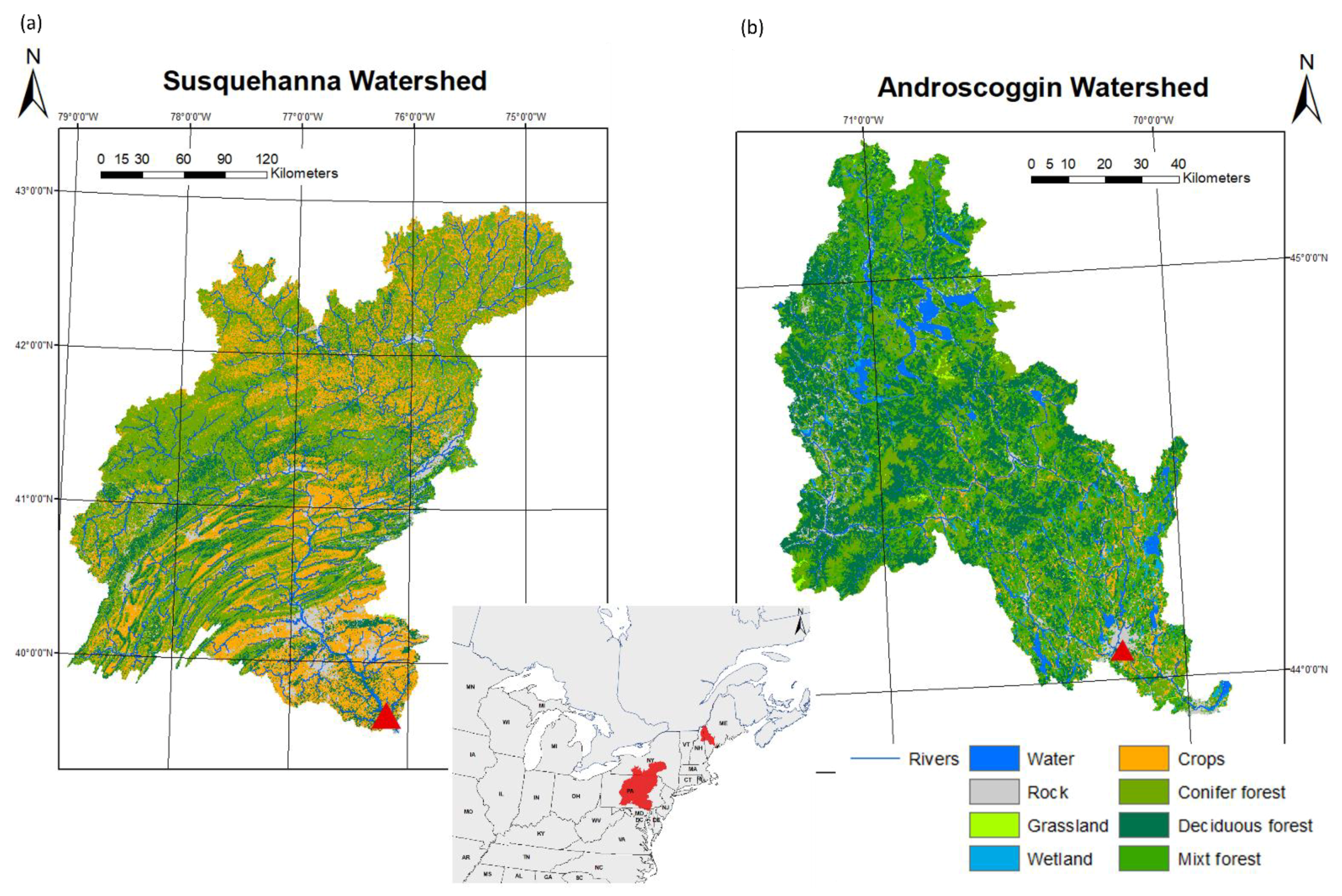
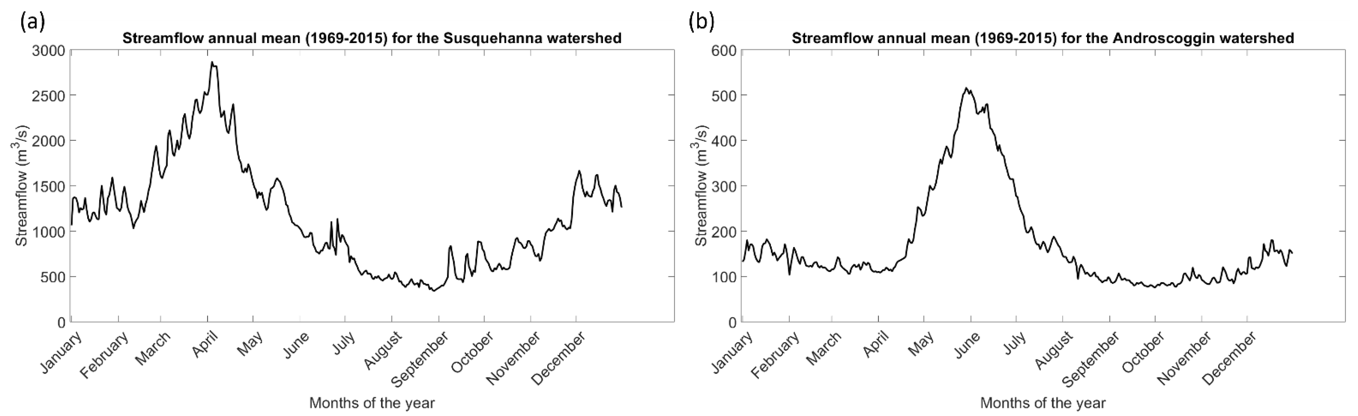
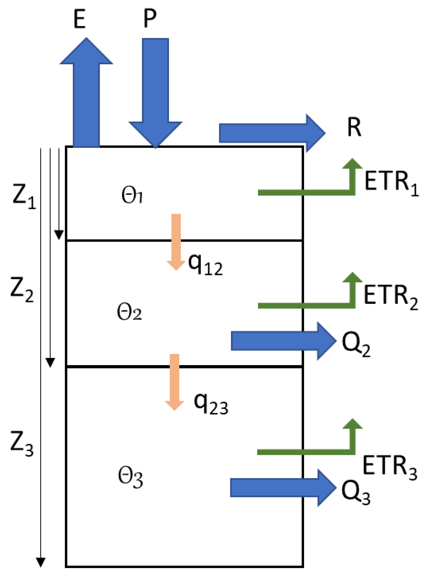
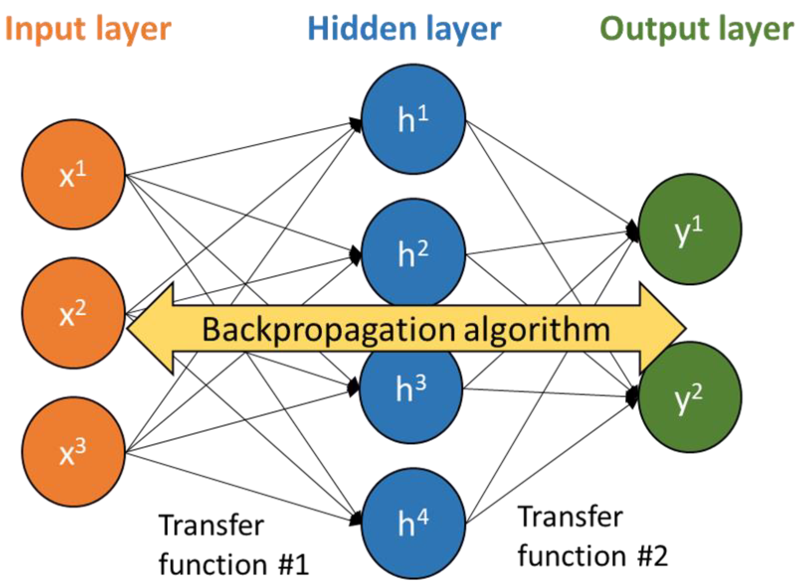
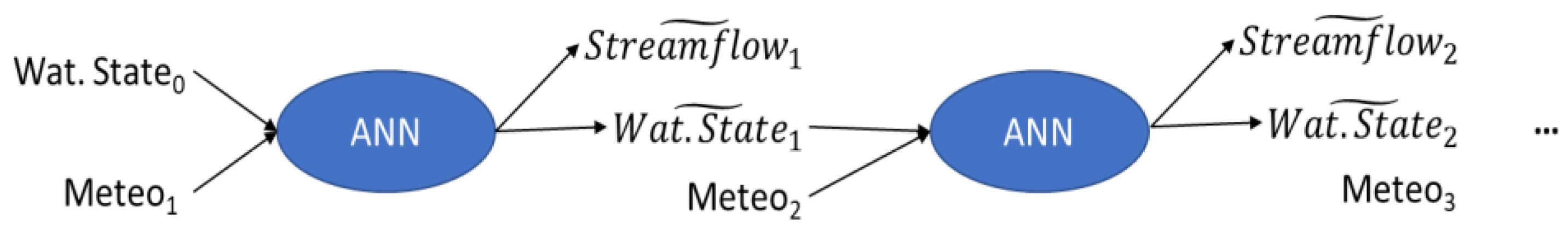
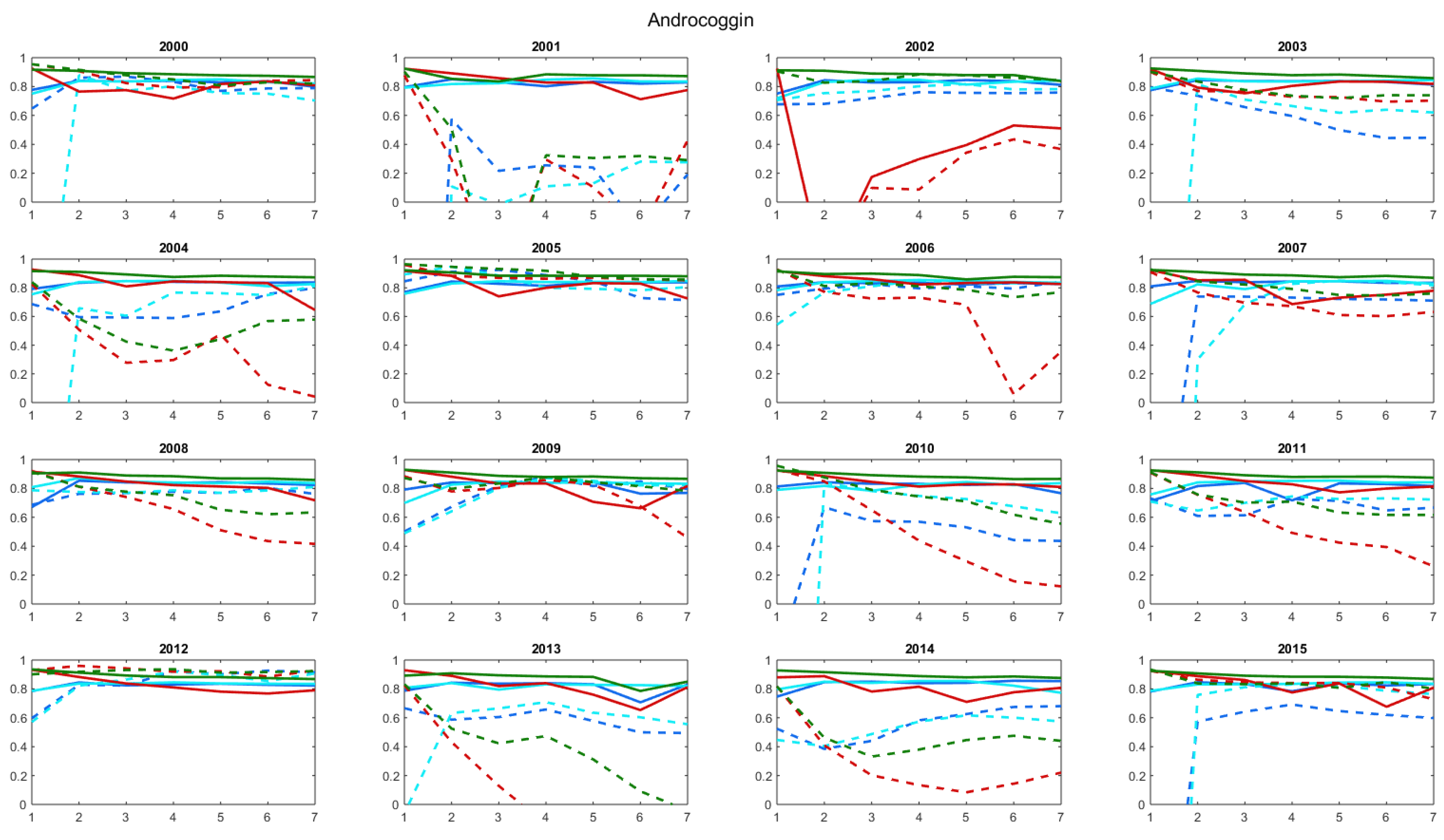
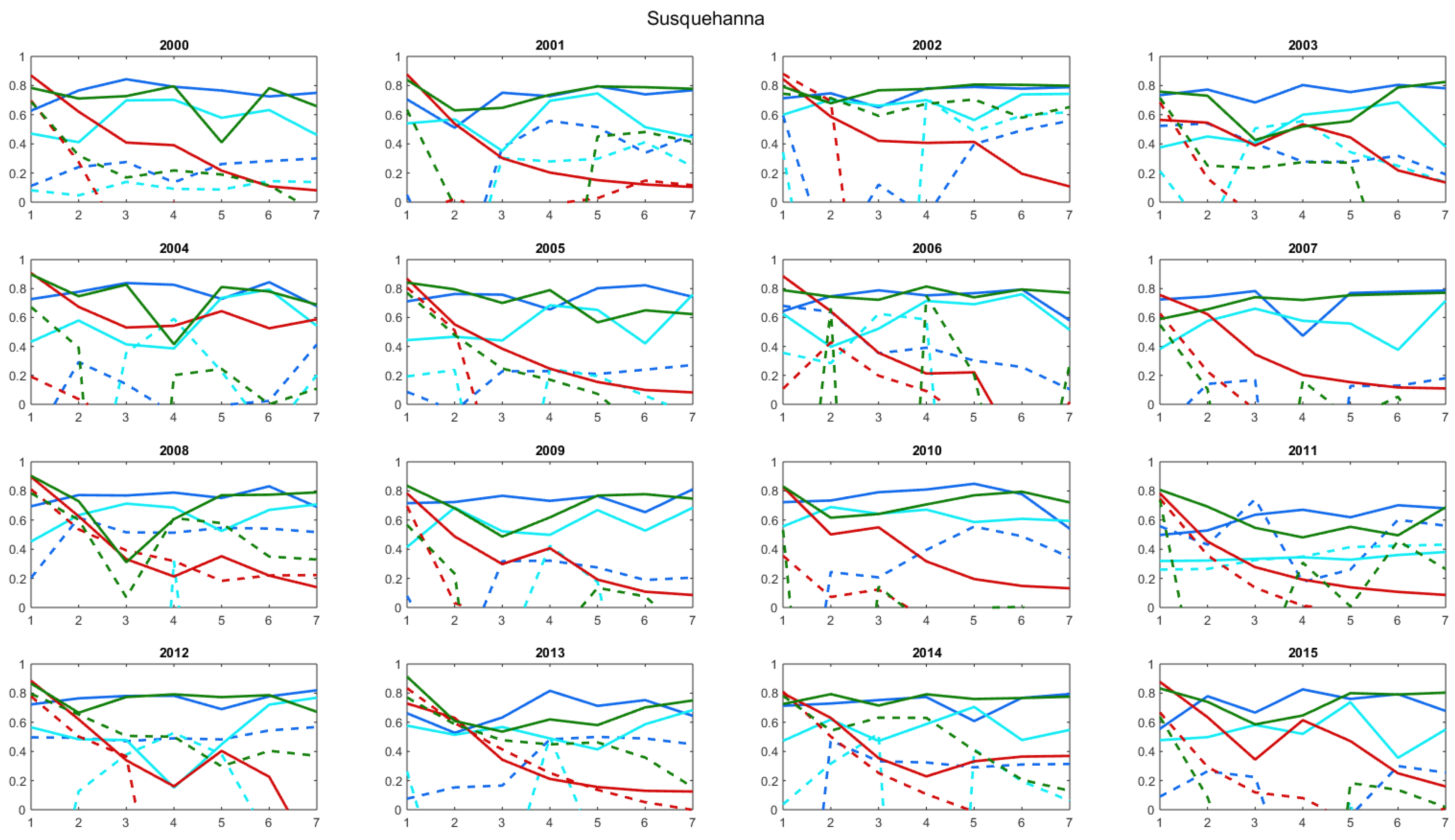
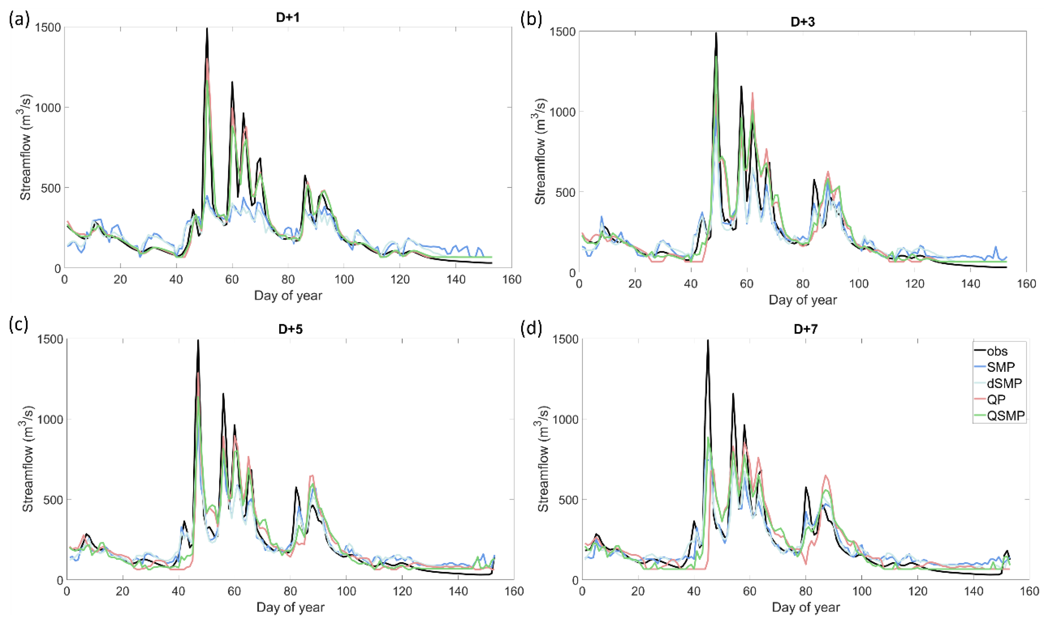
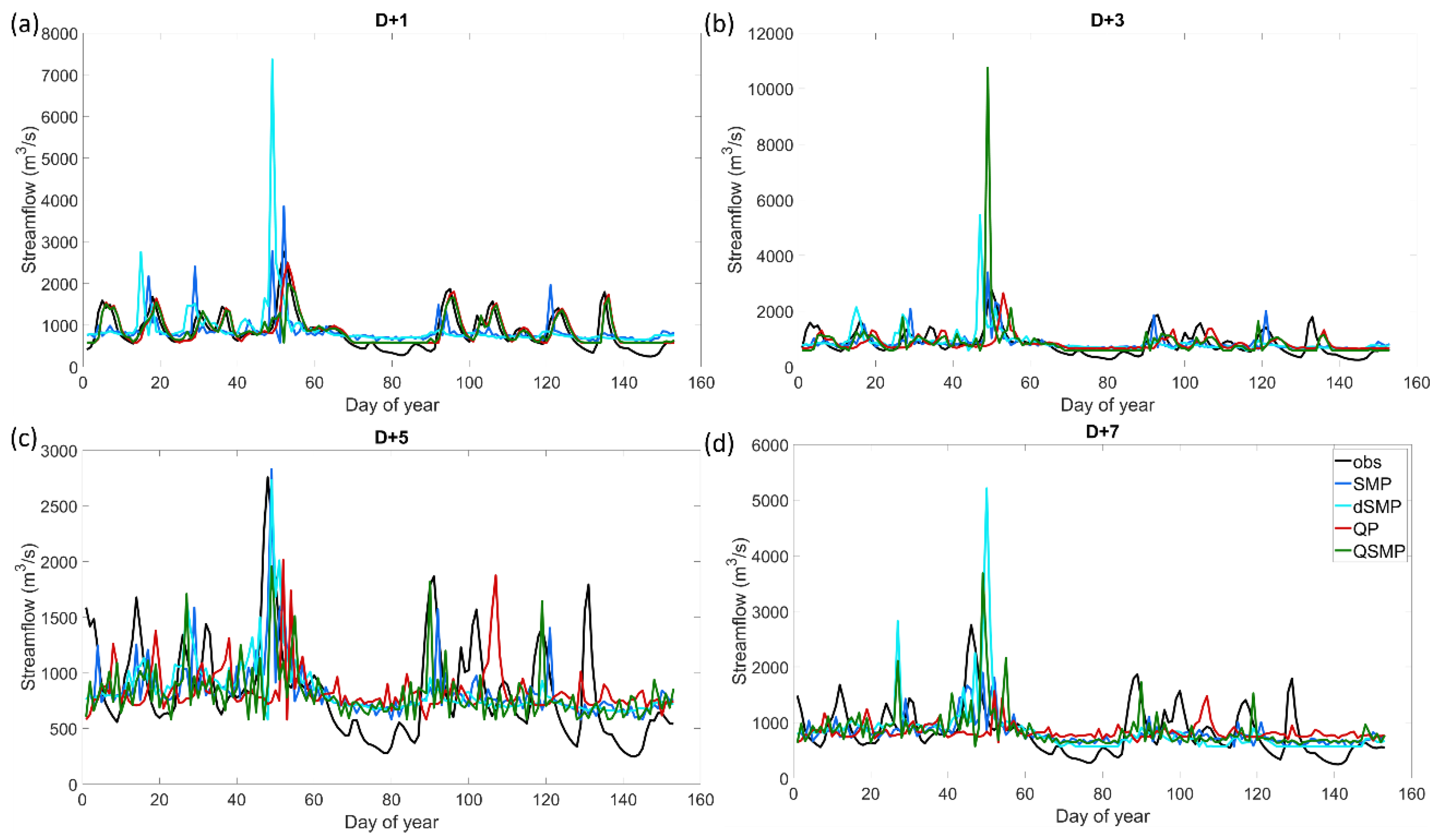
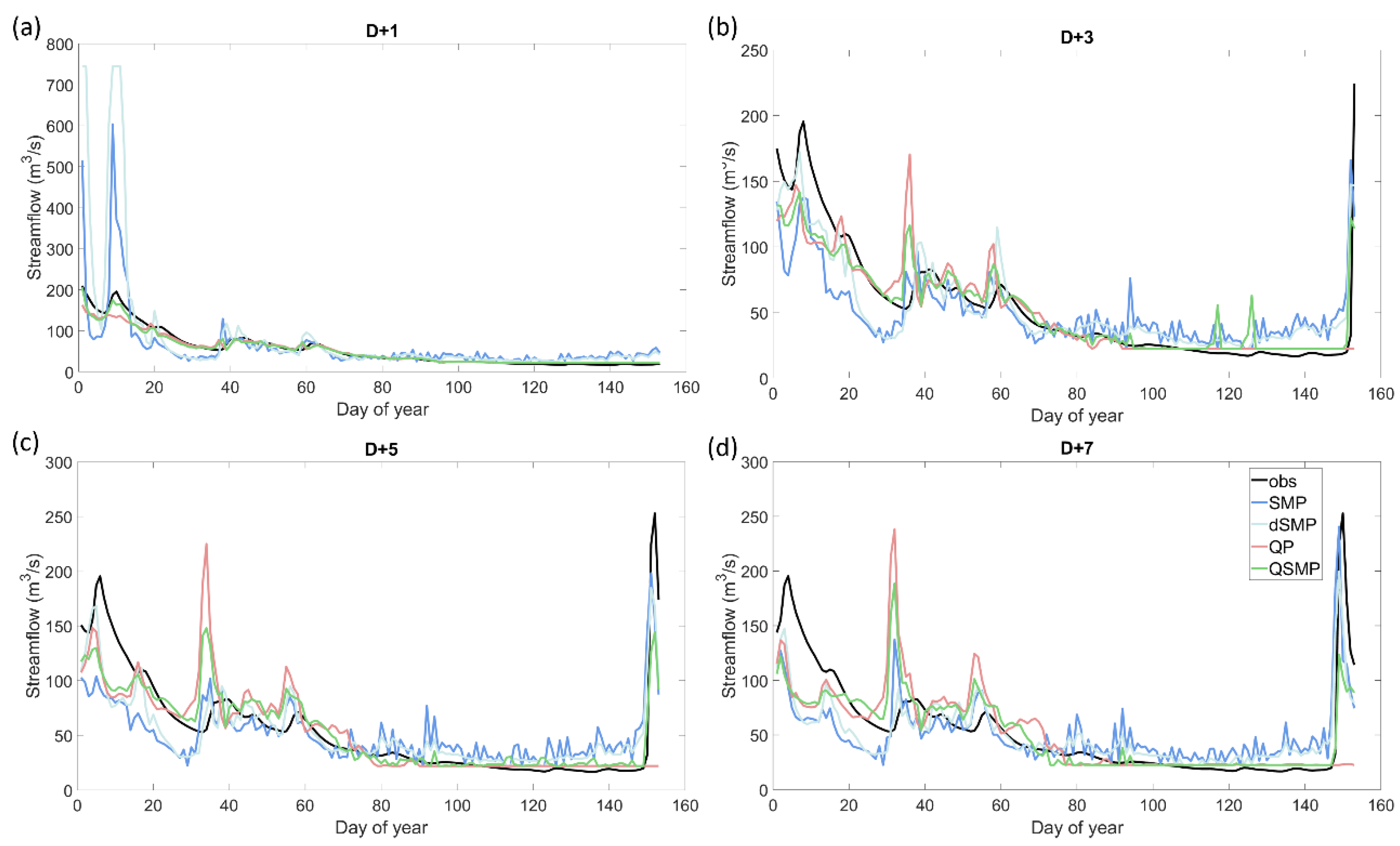
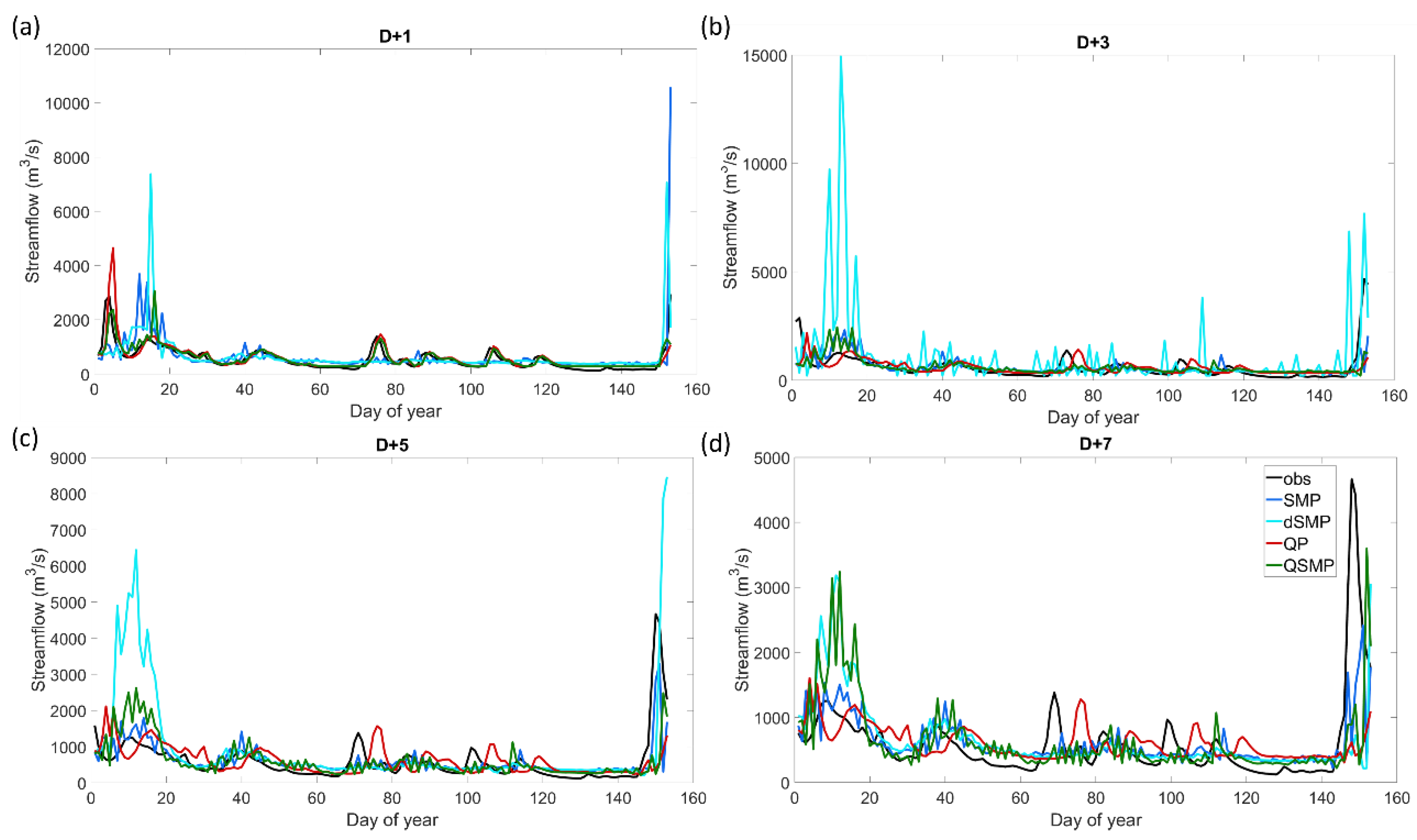
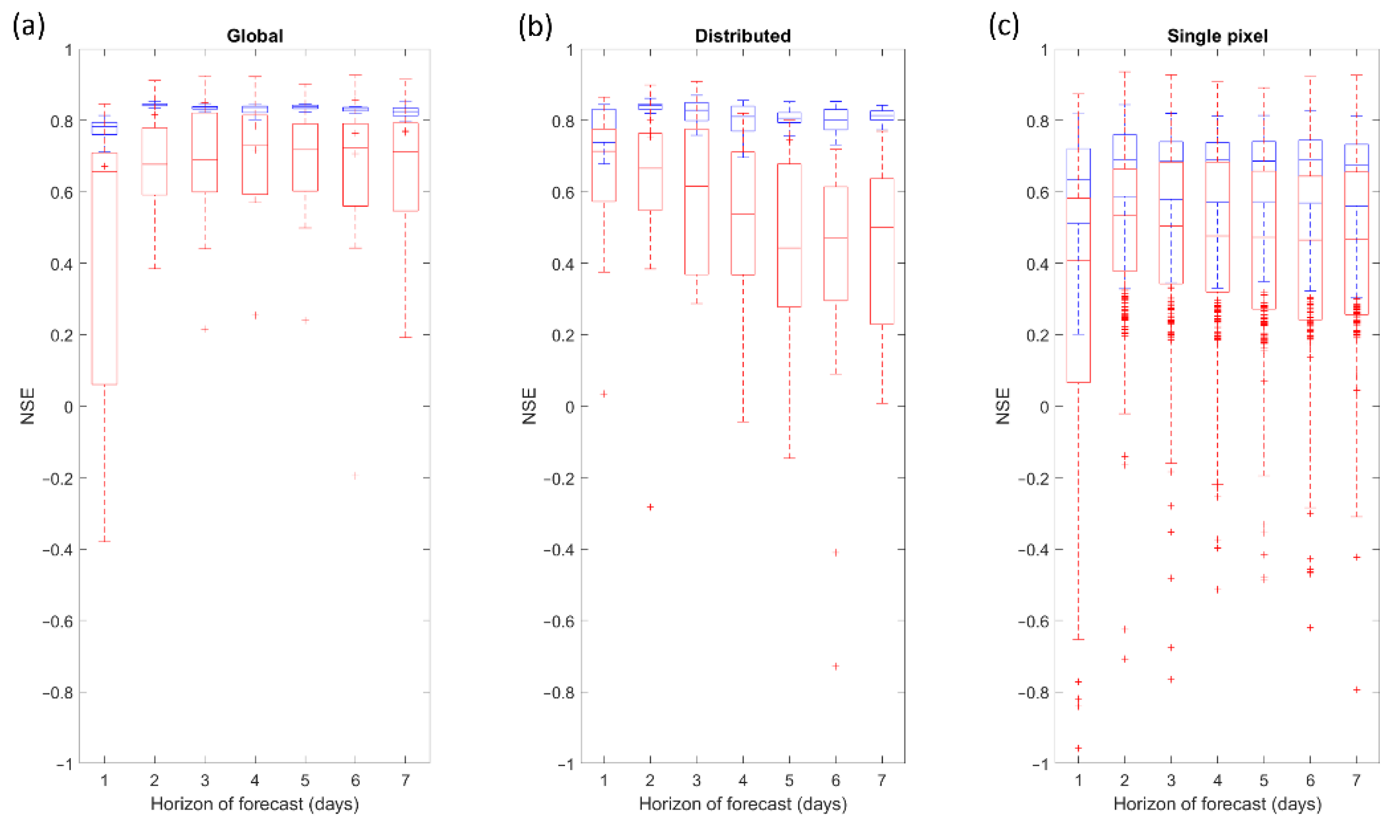
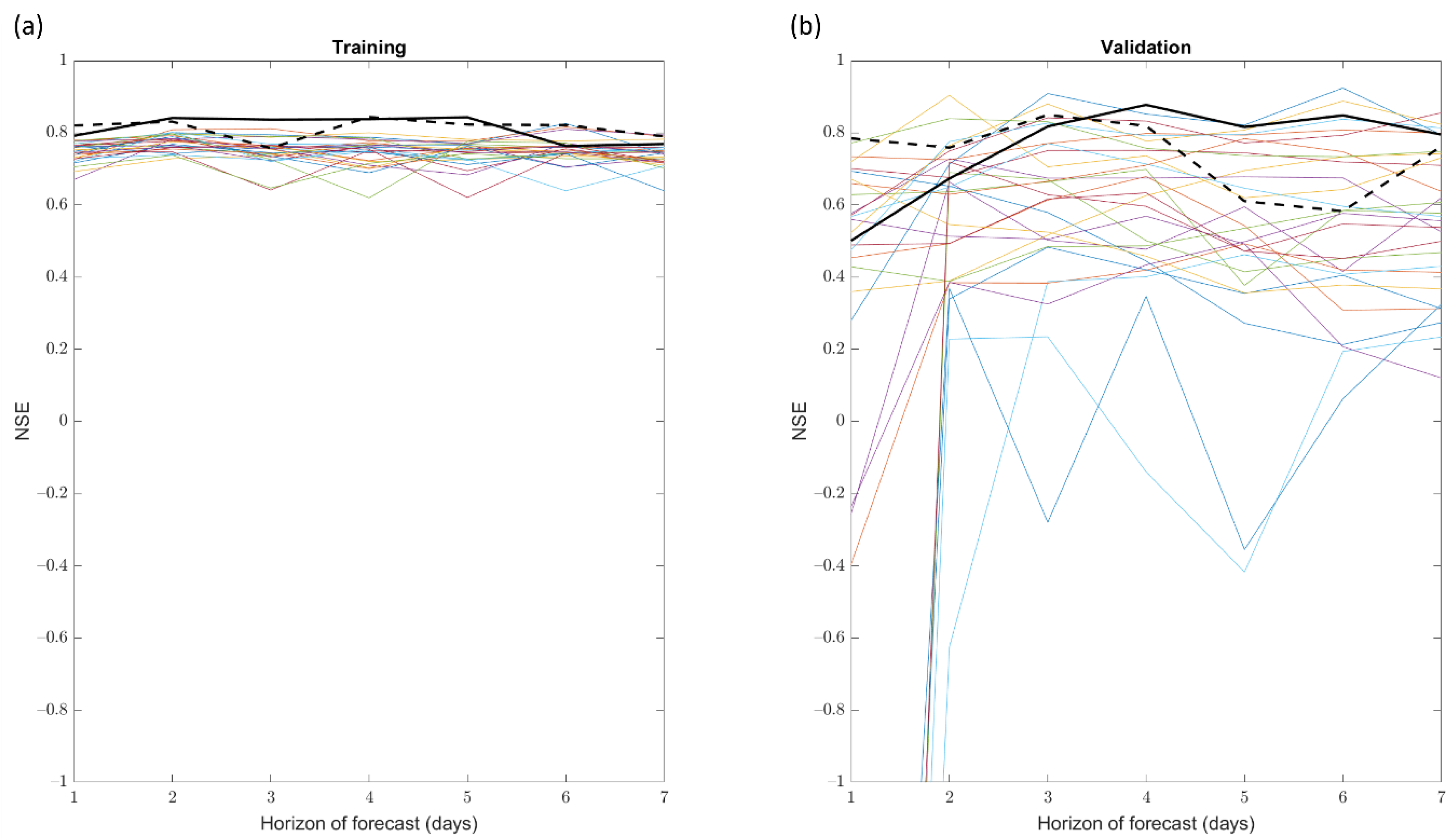
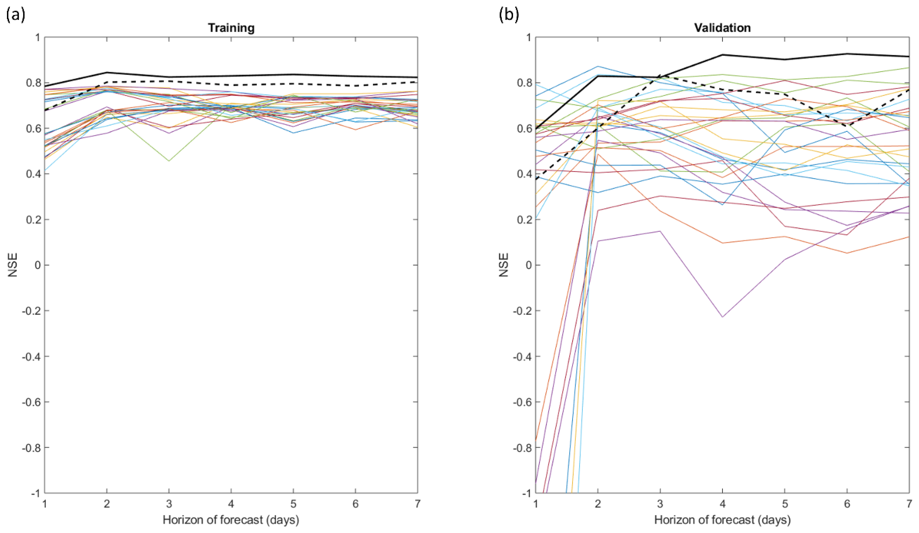
Table 1.
Return streamflow for four specific return periods: 2, 10, 25, and 100 years for the two watersheds, generated with datasets covering 47 years (1969–2015).
Table 1.
Return streamflow for four specific return periods: 2, 10, 25, and 100 years for the two watersheds, generated with datasets covering 47 years (1969–2015).
| Watershed | Q2 (m3/s) | Q10 (m3/s) | Q25 (m3/s) | Q100 (m3/s) |
|---|---|---|---|---|
| Androscoggin | 161 | 424 | 556 | 751 |
| Susquehanna | 939 | 2772 | 3695 | 5059 |
Table 2.
Summary of HYDROTEL’s defined sub-models and associated simulation options. Simulation options used in this study to generate hydrometeorological ‘observations’ are bolded.
Table 2.
Summary of HYDROTEL’s defined sub-models and associated simulation options. Simulation options used in this study to generate hydrometeorological ‘observations’ are bolded.
| Sub-Models | Simulation Options |
|---|---|
| Interpolation of precipitation | Thiessen polygon |
| Weighted mean of nearest 3 stations | |
| Snowmelt | Modified Degree-day |
| Evapotranspiration | Thornthwaite |
| Linacre | |
| Penman | |
| Priestley-Taylor | |
| Hydro-Québec | |
| Vertical water budget | CEQUEAU |
| Three-Layer Vertical Budget (BV3C) | |
| Surface and subsurface runoff | Kinematic wave equation |
| Channel routing | Modified kinematic wave equation |
| Diffusive wave equation |
Table 3.
Combinations of variables defined as artificial neural network (ANN) inputs.
| No. and Name | Watershed State Variables | Meteorological Variables |
|---|---|---|
| At Day D-1 | At Day D and Day D-1 | |
| 1—QP | Downstream Streamflow | Precipitation |
| 2—SMP | Surface Soil Moisture | Precipitation |
| 3—dSMP | Deep Soil Moisture | Precipitation |
| 4—QSMP | Downstream Streamflow | Precipitation |
| Surface Soil Moisture |
Table 4.
Number of inputs for the ANN model depending on the combination of variables and the spatial distribution. With a regular grid, information is only given for the Androscoggin watershed (An.).
Table 4.
Number of inputs for the ANN model depending on the combination of variables and the spatial distribution. With a regular grid, information is only given for the Androscoggin watershed (An.).
| No. and Name | Average | Regular Grid |
|---|---|---|
| 1—SMP | ||
| 2—dSMP | 3 | 84 (An.) |
| 3—QP | ||
| 4—QSMP | 4 | 112 (An.) |
Table 5.
Nash–Sutcliffe efficiency (NSE) values for Susquehanna and Androscoggin for summer 2009, a relatively wet year, as validation period.
Table 5.
Nash–Sutcliffe efficiency (NSE) values for Susquehanna and Androscoggin for summer 2009, a relatively wet year, as validation period.
| Watershed | Susquehanna | Androscoggin | |||||||
|---|---|---|---|---|---|---|---|---|---|
| Forecast Horizon | D + 1 | D + 3 | D + 5 | D + 7 | D + 1 | D + 3 | D + 5 | D + 7 | |
| 1-QP | train. | 0.784 | 0.298 | 0.192 | 0.086 | 0.928 | 0.835 | 0.707 | 0.818 |
| valid. | 0.696 | −0.057 | −0.328 | −0.116 | 0.884 | 0.803 | 0.827 | 0.458 | |
| 2-SMP | train. | 0.716 | 0.767 | 0.765 | 0.812 | 0.792 | 0.837 | 0.843 | 0.769 |
| valid. | 0.080 | 0.318 | 0.274 | 0.205 | 0.501 | 0.818 | 0.816 | 0.796 | |
| 3-dSMP | train. | 0.415 | 0.523 | 0.669 | 0.685 | 0.699 | 0.847 | 0.842 | 0.833 |
| valid. | −1.321 | −0.369 | 0.175 | −0.603 | 0.489 | 0.803 | 0.852 | 0.824 | |
| 4-QSMP | train. | 0.835 | 0.486 | 0.768 | 0.747 | 0.930 | 0.887 | 0.883 | 0.867 |
| valid. | 0.567 | −2.163 | 0.135 | −0.215 | 0.873 | 0.834 | 0.844 | 0.783 | |
Table 6.
NSE values for Susquehanna and Androscoggin for summer 2010, a relatively dry year as validation period.
Table 6.
NSE values for Susquehanna and Androscoggin for summer 2010, a relatively dry year as validation period.
| Watershed | Susquehanna | Androscoggin | |||||||
|---|---|---|---|---|---|---|---|---|---|
| Forecast Horizon | D + 1 | D + 3 | D + 5 | D + 7 | D + 1 | D + 3 | D + 5 | D + 7 | |
| 1-QP | train. | 0.828 | 0.550 | 0.195 | 0.132 | 0.924 | 0.846 | 0.829 | 0.810 |
| valid. | 0.355 | 0.123 | −0.114 | −0.061 | 0.928 | 0.650 | 0.295 | 0.122 | |
| 2-SMP | train. | 0.723 | 0.791 | 0.849 | 0.541 | 0.814 | 0.833 | 0.824 | 0.767 |
| valid. | −1.914 | 0.207 | 0.555 | 0.344 | −0.380 | 0.574 | 0.531 | 0.436 | |
| 3-dSMP | train. | 0.556 | 0.643 | 0.586 | 0.595 | 0.790 | 0.784 | 0.844 | 0.837 |
| valid. | −2.189 | −7.368 | −2.631 | −0.261 | −5.375 | 0.782 | 0.727 | 0.628 | |
| 4-QSMP | train. | 0.831 | 0.642 | 0.770 | 0.721 | 0.824 | 0.892 | 0.877 | 0.866 |
| valid. | 0.534 | 0.143 | −0.002 | −0.078 | 0.957 | 0.790 | 0.710 | 0.555 | |
Publisher’s Note: MDPI stays neutral with regard to jurisdictional claims in published maps and institutional affiliations. |
© 2022 by the authors. Licensee MDPI, Basel, Switzerland. This article is an open access article distributed under the terms and conditions of the Creative Commons Attribution (CC BY) license (https://creativecommons.org/licenses/by/4.0/).
Share and Cite
MDPI and ACS Style
Jougla, R.; Leconte, R. Short-Term Hydrological Forecast Using Artificial Neural Network Models with Different Combinations and Spatial Representations of Hydrometeorological Inputs. Water 2022, 14, 552. https://doi.org/10.3390/w14040552
AMA Style
Jougla R, Leconte R. Short-Term Hydrological Forecast Using Artificial Neural Network Models with Different Combinations and Spatial Representations of Hydrometeorological Inputs. Water. 2022; 14(4):552. https://doi.org/10.3390/w14040552
Chicago/Turabian StyleJougla, Renaud, and Robert Leconte. 2022. "Short-Term Hydrological Forecast Using Artificial Neural Network Models with Different Combinations and Spatial Representations of Hydrometeorological Inputs" Water 14, no. 4: 552. https://doi.org/10.3390/w14040552
Note that from the first issue of 2016, this journal uses article numbers instead of page numbers. See further details here.