
Impacts of Rainfall Data Aggregation Time on Pluvial Flood Hazard in Urban Watersheds


1
Department of Civil and Environmental Engineering, University of Florence, 50139 Florence, Italy
2
Department of Civil and Environmental Engineering, University of Perugia, 06125 Perugia, Italy
*
Author to whom correspondence should be addressed.
Water 2022, 14(4), 544; https://doi.org/10.3390/w14040544
Submission received: 5 January 2022
/
Revised: 3 February 2022
/
Accepted: 7 February 2022
/
Published: 11 February 2022
(This article belongs to the Special Issue Time-Resolution of Rainfall Data and Its Role in the Hydrological Analyses)
Abstract
:Pluvial floods occur when heavy rainstorms cause the surcharge of the sewer network drainage, representing one of the most impacting natural hazard in urban watersheds. Pluvial flood hazard is usually assessed considering the effect of annual maxima rainfall of short duration, comparable with the typical concentration times of small urban watersheds. However, short duration annual maxima can be affected by an error of underestimation due to the time resolution as well as the aggregation time of the rainfall time series. This study aims at determining the impact of rainfall data aggregation on pluvial flood hazard assessment. Tuscany region (Central Italy) is selected as a case study to perform the assessment of the annual maxima rainfall underestimation error, since the entire region has the same temporal aggregation of rainfall data. Pluvial flood hazard is then evaluated for an urban watershed in the city of Florence (Tuscany) comparing the results obtained using observed (uncorrected) and corrected annual maxima rainfall as meteorological forcing. The results show how the design of rainfall events with a duration of 30 min or shorter is significantly affected by the temporal aggregation, highlighting the importance of correcting annual maxima rainfall for a proper pluvial flood hazard evaluation.
1. Introduction
Increasingly dense urban development is causing major difficulties worldwide to cope with sudden and intense rainfall events of short durations. These kinds of events cause the surcharge of the sewer network overcoming its drainage capacity (i.e., pluvial flooding [1,2]). Moreover, climate change is expected to exacerbate weather-related hazards, increasing the number and frequency of extreme rainfall events that can cause urban pluvial flood events [3,4,5].
In the last decade, pluvial flood risk management has been rapidly evolving [6,7], with multiple assessment frameworks developed exploring the geophysical, economical and social dimensions [8,9,10]. The effective analysis of pluvial flood hazard (i.e., quantitatively defining rainfall events and their flood impact in a spatially explicit manner [11]) requires an accurate simulation of precipitation events with their corresponding frequencies [12]. Pluvial flood analysis is usually carried out using hydrologic and hydraulic models in which the precipitation, usually of sub-hourly duration, is among the main influencing factors [13,14,15].
Indeed, pluvial flood events are usually associated with rainfall events characterized by short duration (less than 3 h) and high intensity (more than 30 mm/h) [16,17,18]. Therefore, the correct estimation of rainfall depth becomes essential to effectively evaluate the associated pluvial flood hazard.
Several issues can compromise the correct rainfall estimation, such as the relocation of gauge stations, the use of different rain gauge types, and the change of gauge station surroundings, determining relevant effects on many related investigations including the evolution of extreme rainfall trends and the determination of rainfall depth–duration–frequency curves [19,20].
Among the others, the effect of using time series with coarse aggregation time to estimate maximum rainfall depths represents a major criticality [21], especially when dealing with pluvial hazard. Following the approaches introduced by Young and McEnroe [22] and Yoo et al. [23], conversion factors have been investigated to overcome the issues related to scarce data availability and to allow the use of series with coarse aggregation time. In particular, Morbidelli et al. [21] proposed a methodology to obtain a homogeneous series of annual maximum rainfall depths from data derived through different aggregation times.
With the purpose of contributing towards a better estimation of flood hazard in urban areas, this paper investigates the effects of correcting historical extreme rainfall series to improve the accuracy of flood-prone areas mapping. First, the rainfall series correction procedure developed by Morbidelli et al. [21] is adopted and applied to the Tuscany Region to refine the design rainfall events estimation. Second, a rainfall-runoff model is used to evaluate the effects of corrected meteorological forcing on pluvial flood hazard assessment in a specific case study (i.e., City of Florence, Central Italy). The assessment is carried out comparing the output obtained in corrected and uncorrected scenarios with multiple event durations and magnitudes. Finally, the results are discussed, analyzing the effectiveness of the proposed approach to better forecast the potential drainage network criticalities and to improve the flooded area delineation.
2. Case Study
This study embeds two parts with two different case studies. First, the underestimation of the annual maxima caused by the time of aggregation of the rainfall time series is evaluated at the regional scale. In this first part, the study area is the Tuscany Region (Central Italy), where the whole rain gauge network is managed by the same Hydrological Regional Service (HRS). Even if there are differences within the recording resolution of the rain gauge network (Figure 17 in [24]), the automatic rain gauges installed in the last 20 years have the same aggregation time ta. For this reason, all the rain gauges are affected by the same errors. The second part of this study is focused on an urban watershed in the city of Florence in Tuscany. The watershed is used as a target area to test the impact of the annual maxima rainfall correction on the sewer system modeling and pluvial flood hazard estimation.
2.1. Tuscany Region
The history of the rainfall data time of aggregation in Tuscany was previously described in the work of Morbidelli et al. [24]. In that study, the description of the rain gauges network shows how in recent years almost all the gauge stations have been transformed or are installed—in case of new installations—as automatic with a 1 min time resolution. Nevertheless, this resolution represents the capability of the rain gauge of providing the measurements only. Indeed, the raw data must be analyzed, then post-processed, and in this last procedure part of the information can be lost. In Tuscany, the actual finest data available, provided by the HRS, are rainfall series with a 15 min-time step. Actually, the time of aggregation of rainfall data has been changed and has been improved with the technology over time, as already mentioned in Morbidelli et al. [24]. Nonetheless, starting from the beginning of the 1980s, the time of aggregation is not constrained by the rain gauges technology, but it is arbitrarily set by the HRS. Such a decision is driven by the optimization of the data post-processing.
Figure 1 shows the annual maxima series published by the HRS of the Tuscany regions for two rain gauges (Porrino and Polla dei Gangheri), as an example. The temporal aggregation of the rainfall data changed in the last year from 10 to 15 min. From 1976 to 1985 (red filled box in Figure 1), it is not completely clear how the data were post-processed, since the temporal aggregation seems to be different within the rain gauges network. Some stations in some years have a temporal aggregation of 10 min and also the maxima in the duration of 20 min are available, some others have a temporal aggregation of 15 min. During the years 1986, 1987, 1988, and 1989 the time of aggregation of rainfall series was set to 5 min within all the rain gauge network and the maximum rainfall for all the durations were available (green filled box in Figure 1). Then, the time of aggregation has increased over time, progressively, losing information. First, up to 10 min in the 1990 (blue filled box in Figure 1), and from 1998–1999 the temporal aggregation was set up to 15 min until now (yellow filled box in Figure 1).
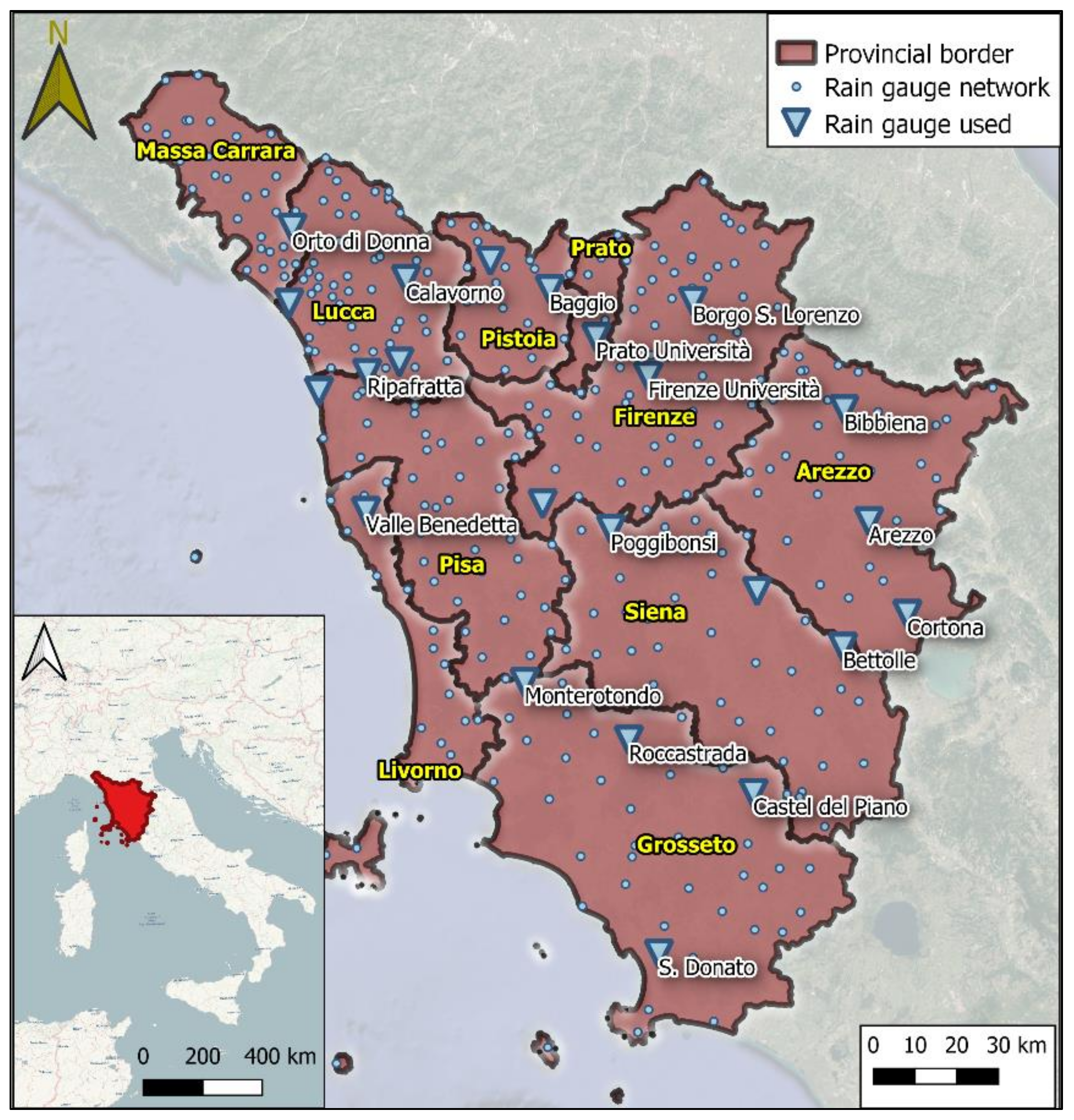
The dataset used to evaluate the average error of underestimation of the annual maximum consists of 23 rain gauges, within the Tuscany Region, with a time of aggregation of 15 min, which represents the aggregation time of the observations, The rain gauges have been chosen following two criteria: the rain gauges evenly cover the regional territory; the rain gauges must have at least a rainfall time series length of 20 years, as suggested by Morbidelli et al. [21]. All selected gauges have a time series that range from 1998 to 2020. The dataset spatial distribution is illustrated in Figure 2, where the selected rain gauges within the rainfall network are represented with blue triangles.
2.2. Florence Urban Watershed
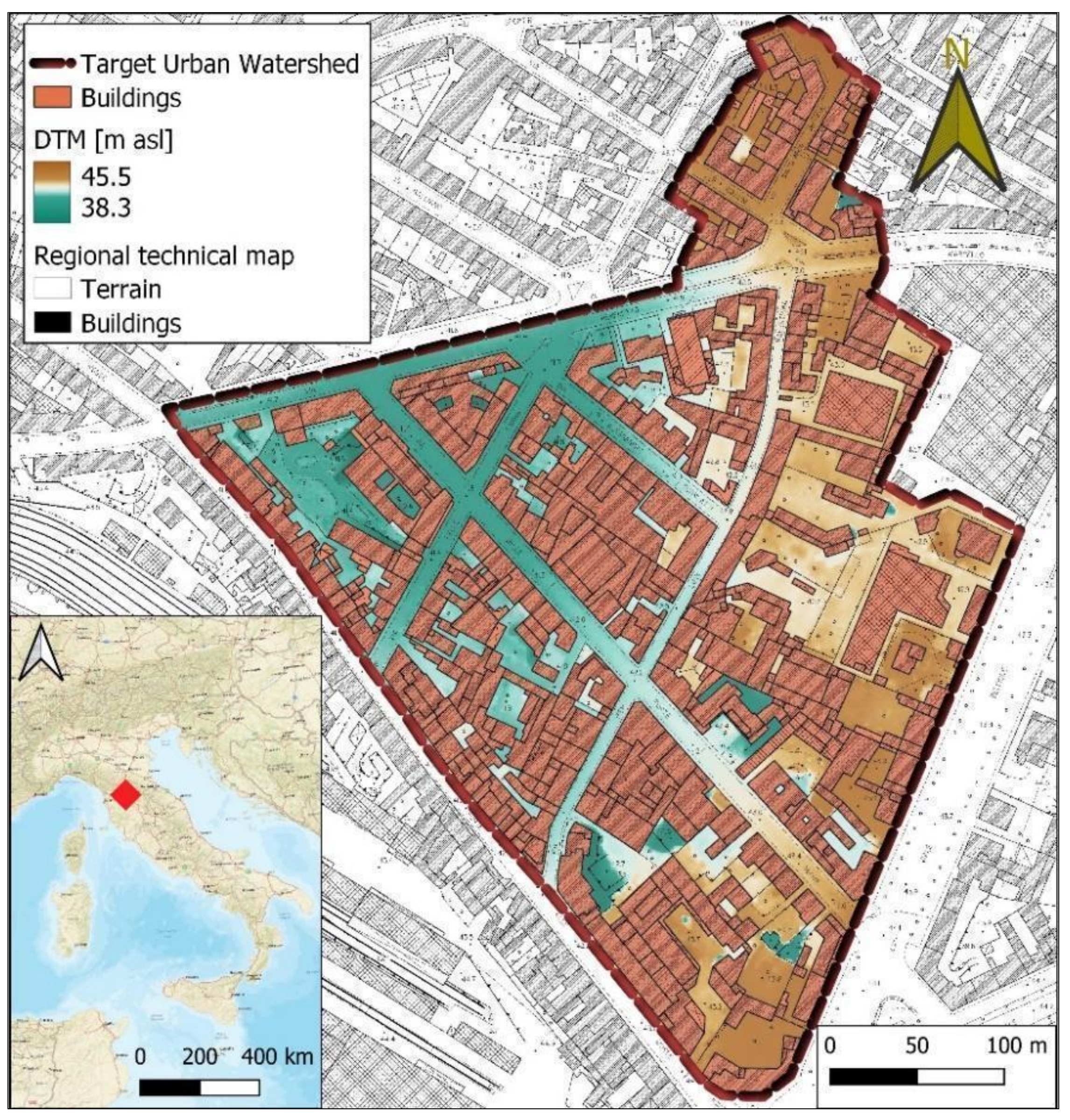
The implications of the usage of the corrected design rainfalls have been evaluated on a Target Urban Watershed (TUW). The TUW is located in Florence’s downtown (Figure 3). The high level of urbanization and the topographical features—presence of depressed zones—of this area makes it exceptionally prone to be flooded during heavy rainstorms.
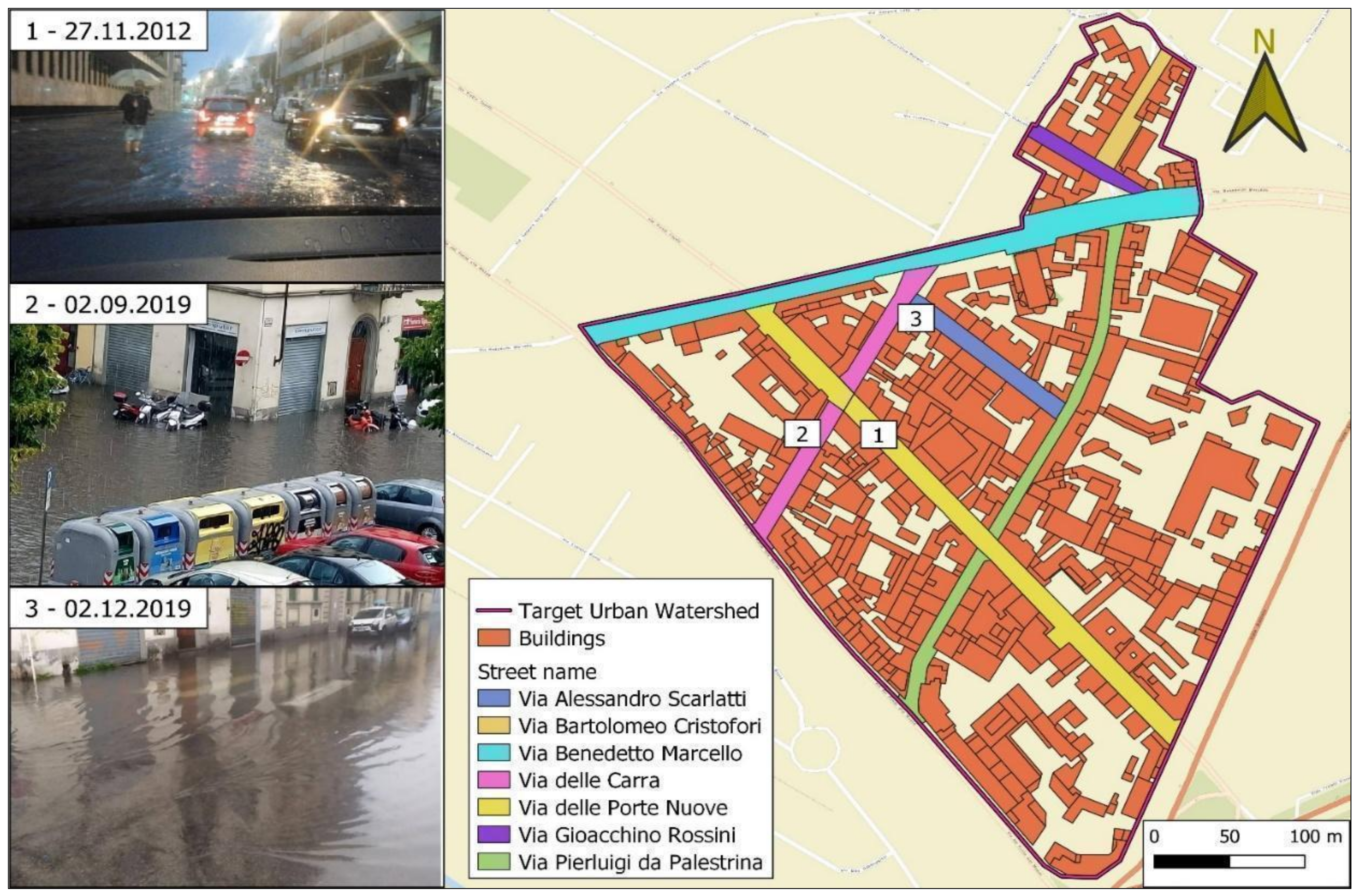
Several flooding events have been registered in this area, with an increasing frequency in the past decade. Three events that occurred, respectively, in November 2012, September 2019 and December 2019 were severe, which produced consistent inundations of the streets with several tens of centimeters water depth (Figure 4).
3. Methodology
The methodology is divided into three parts: (i) evaluation of the underestimation error of the annual maxima rainfall (Section 3.1); (ii) correction of the rainfall series with the evaluation of the design rainfall (Section 3.2) and (iii) hydraulic modelling of the urban watershed to evaluate the pluvial flood hazard.
3.1. Underestimation of the Annual Maxima Rainfall Depth
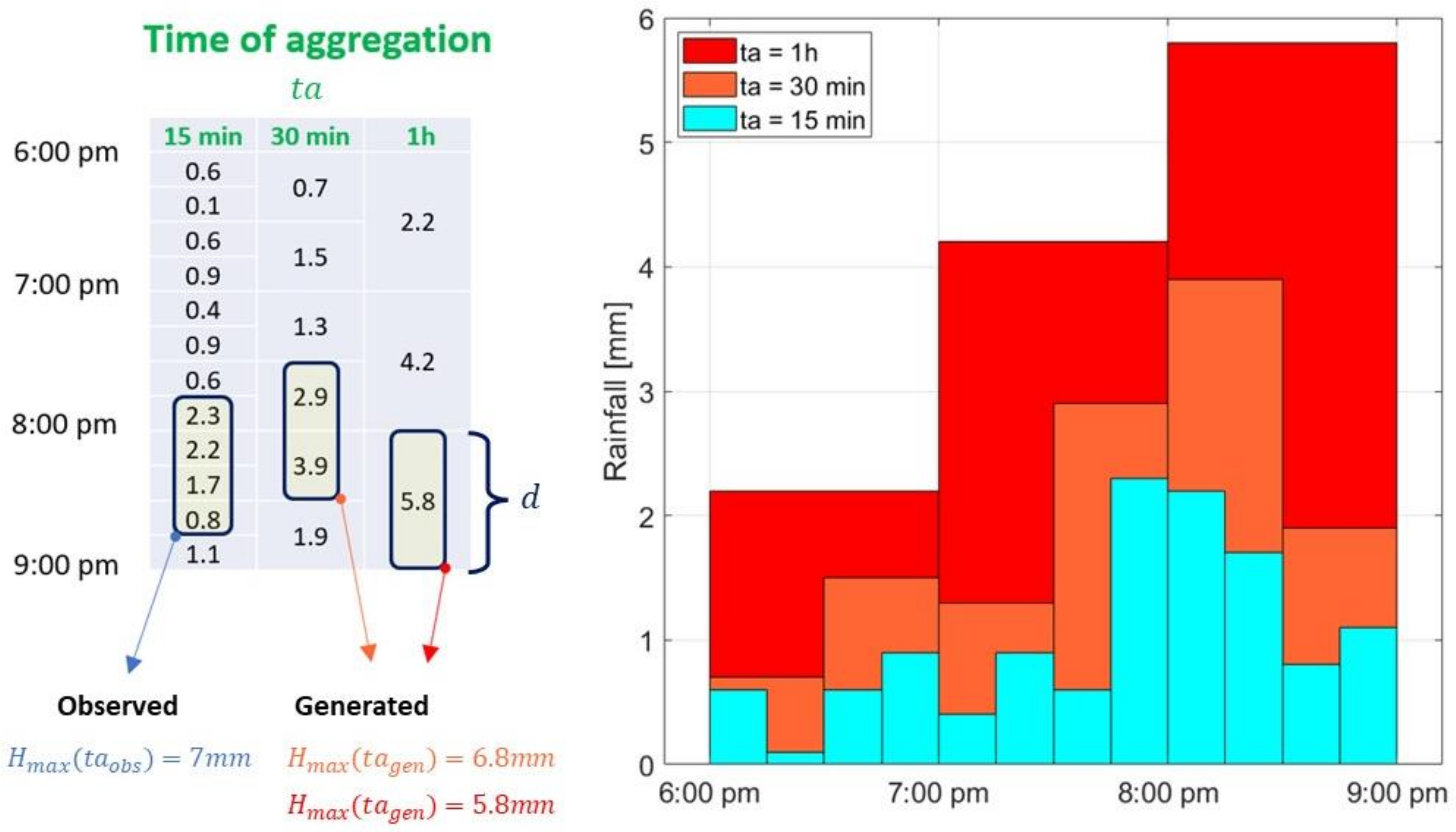
The underestimation error of the annual maxima rainfall depends on the relation between the duration d of the maximum and the time of aggregation ta of the rain gauge network that is used to evaluate the maximum [21,22,23]. For instance, Figure 5 shows how the maximum with a duration d of 1 h is evaluated with different time of aggregations ta (15 min, 30 min, 1 h).
The first step to evaluate the underestimation error of the annual maxima is to use the finer time resolution available, in order to generate new time series with different times of aggregation ta.
The methodology adopted in this section follows the one proposed by Morbidelli et al. [21], with the exception of the finer time resolution available to generate the new time series. For this reason, just the most important aspects of the procedure are described, while further details can be found in Morbidelli et al. [21]. In this study, a 15 min ( time series is aggregated to generate new rainfall time series of duration 30 min, 1 h, 3 h, 6 h, 12 h, 24 h (. Therefore, in each time series, the number of observations per year decreases as the time of aggregation increases. In this framework, the 24 h time series represents the cumulated daily rainfall. Figure 5 shows an example of how the rainfall records have been aggregated.
After the generation of the new time series, the annual maxima rainfall is estimated for each time of aggregation. The annual maxima rainfall, estimated with a finer time of aggregation are more precise. For each year and for each rain gauge station, the annual maxima is estimated with all the generated time series. For each year, all the maxima obtained with the generated time series, , are compared with , the maximum obtained with the finer time series, the observed time series, to evaluate the error of underestimation . The estimation of , for each i-year, is described by the following equation:
Averaging the over the whole time series, an average underestimation error, , is obtained for each gauge station.
Therefore, each rain gauge has a mean error for each duration d and time of aggregation ta. Then, considering the mean errors of all the rain gauges, a median value of the error for a specific duration and time of aggregation, , can be extracted for the entire region. At the same time, also the errors associated at the 95th percentile is considered, , to analyze how a larger underestimation error impacts on the flood hazard assessment.
3.2. Correction of the Rainfall Series and Design Event Estimation
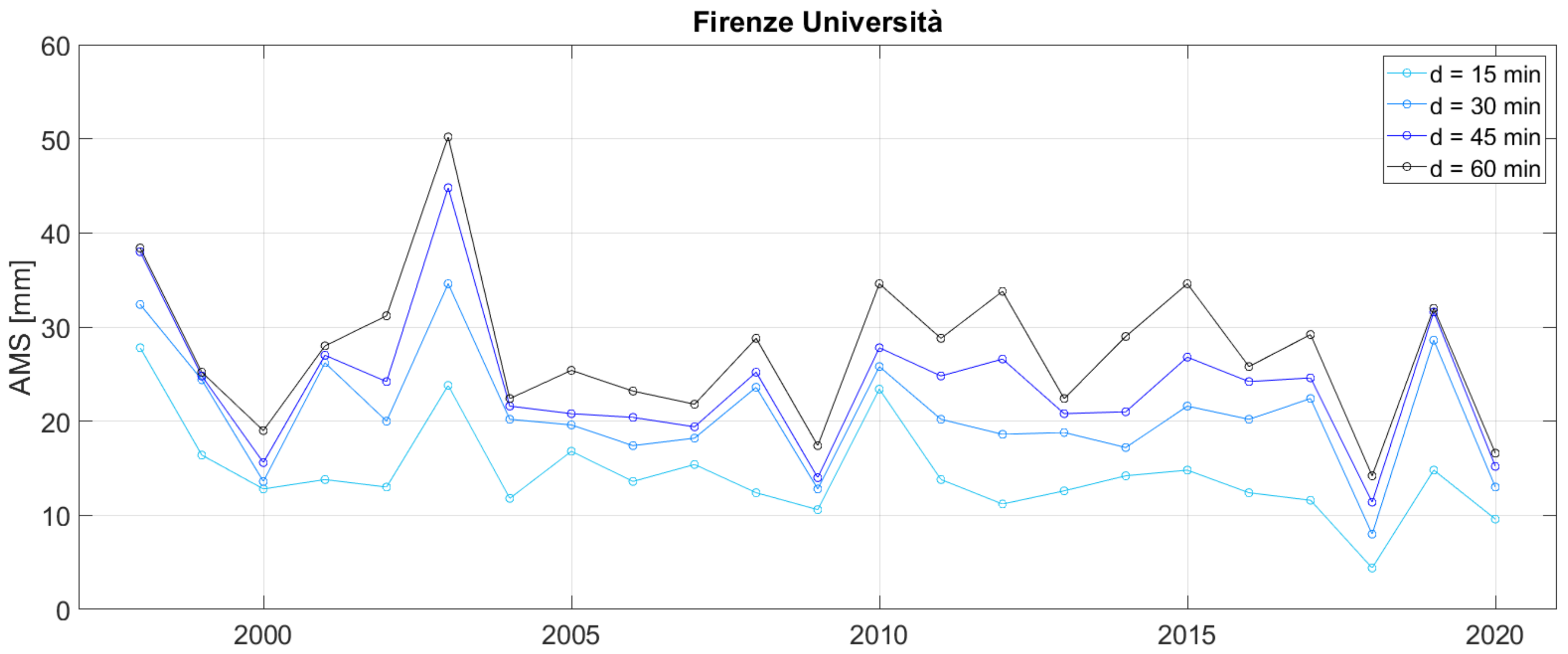
The inputs of the hydrological model are design rainfalls for 4 Return Periods (RP)—2, 5, 10 and 20 years—in four short durations (15, 30, 45 and 60 min). Even if the design rainfalls commonly used in the Tuscany Region are obtained with a Regional Frequency Analysis (Caporali et al. 2018), in this case they have been obtained just fitting a Probability Distribution Function (PDF) on the Annual Maxima Series (AMS) of the rain gauge closest to the urban watershed. The reference rain gauge is named Firenze Università, which is also within the set of the 23 rain gauges that are used to evaluate the correction of the annual maxima rainfall (see Figure 2). The rain gauge has 23 years of observations and the AMS is shown in Figure 6.
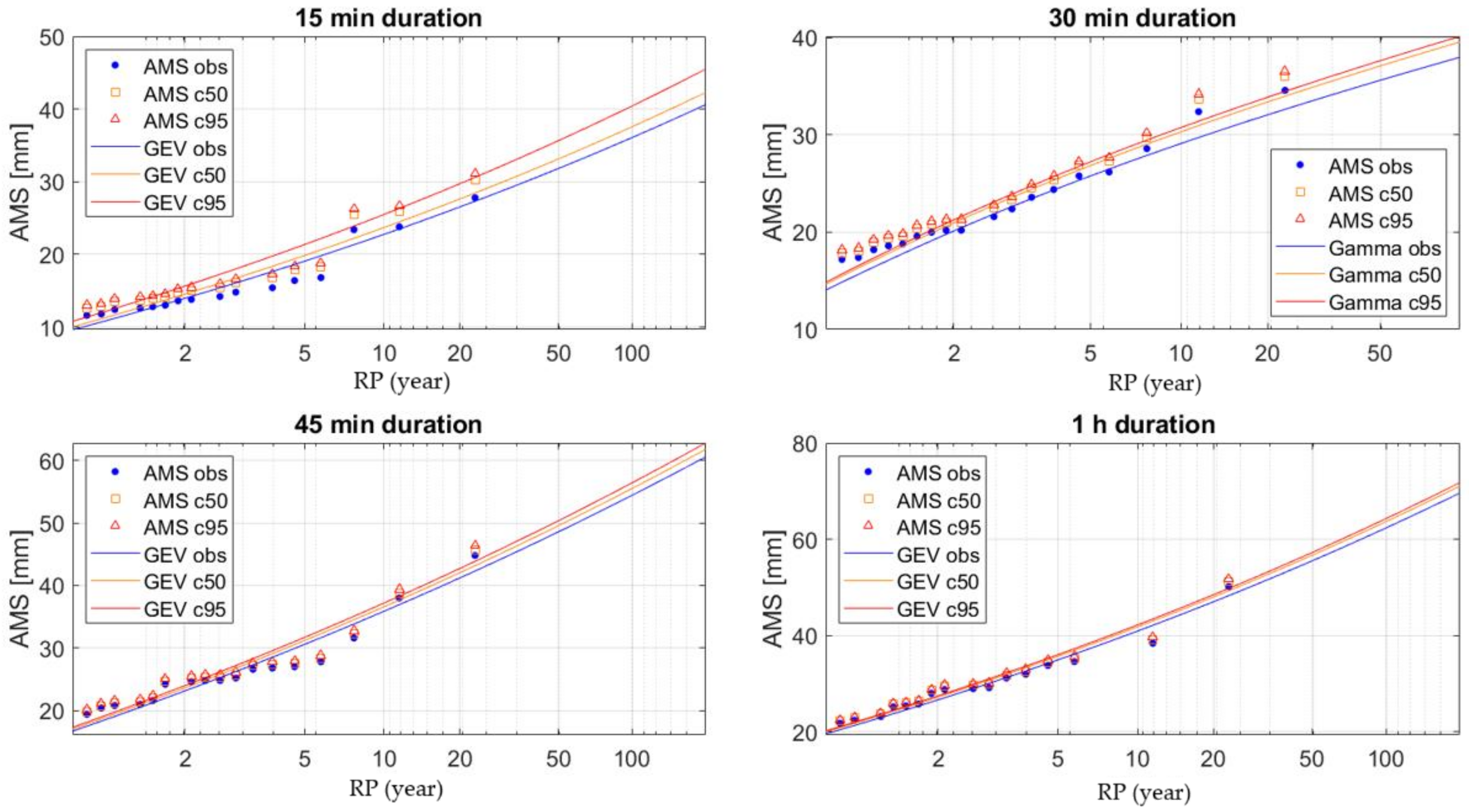
The best PDF for each duration is chosen between the Generalized Extreme Value (GEV) and the Gamma distribution analyzing the Root Mean Squared Error between the data and the curves as objective function. The lowest value of RMSE detected the best fitting for each duration dataset.
After the estimation of the uncorrected design rainfall depths based on the observed time series, by considering the error and and new design rainfalls are obtained for the corrected AMS.
3.3. Hydrological and Hydraulic Modelling of the Urban Watershed
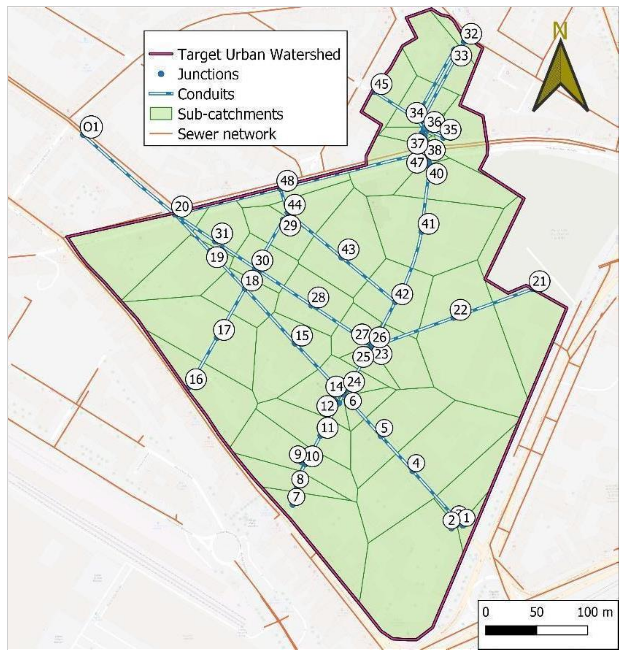
The TUW and its drainage network have been previously analyzed in the study of Giannelli [25]. The hydraulic model of the sewer network has been implemented exploiting the open-source software EPA-SWMM 5.1 [26]. The entire network counts 48 sub-catchments, 49 conduits, 48 junctions and 1 outlet (Figure 7).
The model’s parameters have been calibrated in order to reliably simulate the impacts of the three aforementioned rainfall events (Figure 4), in terms of flooded areas and water depths.
The hydraulic model has been exploited to simulate how the use of uncorrected and corrected precipitation as input affects the assessment of pluvial flood hazard. The outcomes are analyzed in terms of comparisons between the entities of Total Flood Volume (TFV) flowing out from the manholes and flooded areas calculated for the different simulated scenarios.
4. Results and Discussions
This section follows the same scheme as the case study section and it is composed of two parts. First, the results regarding the underestimation error of the AMS and the correction of the design rainfall depths are shown in Section 4.1. Second, the results of the impact of the rainfall data temporal aggregation on the pluvial flood hazard are presented in Section 4.2.
4.1. Hydrological Results
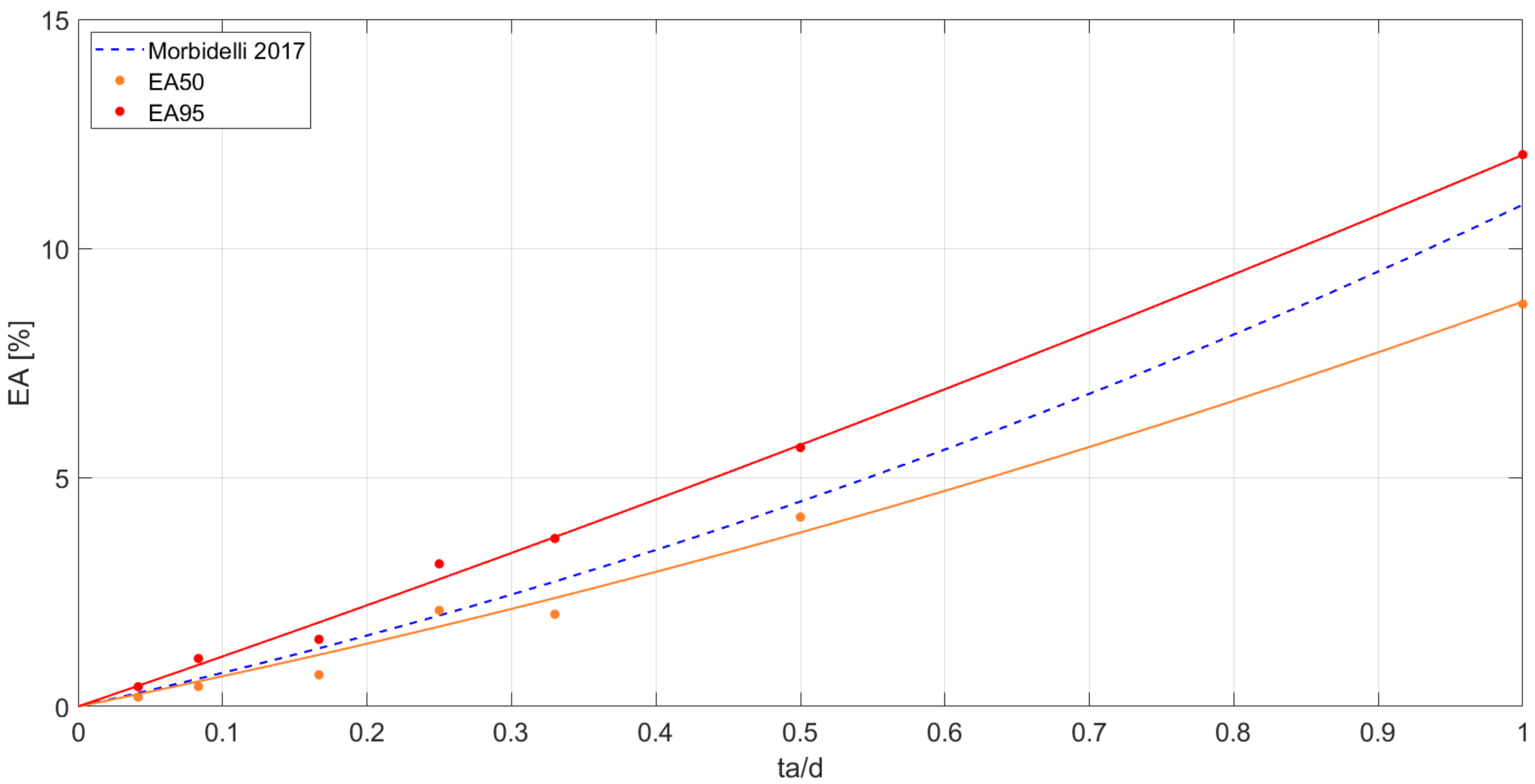
The underestimation of the annual maxima rainfall with a duration d depends on the temporal aggregation ta of the time series. The error has been evaluated for all the time series and with the 23 rain gauge stations in Figure 2. Figure 8 shows the relation of the average error with respect to the ratio between the time of aggregation ta and the duration d. Since the temporal aggregation is constant, and equal to 15 min, the errors associated to each duration can be easily extrapolated from the curves. For instance, a ratio of 0.5 refers to a duration of 30 min.
The associated with the median values of the error is represented in orange; while the correction associated with the 95th percentile is presented in red. The two corrections are expressed by the following equations:
Equations (2) and (3) show how the average error increases with the ratio between the temporal aggregation of the rain gauge station and the duration of the estimated maximum. These equations are valid for all the rain gauges in the region, and they can be used to correct a maximum in the duration d with a temporal aggregation ta of 15 min.
In addition, Figure 8 shows the relation of the average error with respect to the ratio between the temporal aggregation ta and the duration d obtained by Morbidelli et al. [21] (dashed blue line) for the Umbria Region (Central Italy). The relation that describes the underestimation errors of the annual maxima rainfall is slightly lower than the relation by Morbidelli et al. [21], if the median value of the error is considered. Concerning the insights of the aforementioned article, this is a rather expected result, since the aggregation time adopted in Tuscany is much larger than the one used in the Umbria territory.
In this case, the results show how, with the current temporal aggregation of rainfall data, errors of 4% and 9% on the maximum are obtained, respectively, for the duration of 30 and 15 min. At the same time, if the errors associated with the 95th percentile are considered, the percentage of the errors for the same durations rise to 6% and 12%, respectively. The duration of 45 min and 1 h are always affected by a slight error lower than the 5%. Conversely, for a given duration d, the average error decreases accordingly with the reduction of the time of aggregation ta. Thus, improving the aggregation time of the rain gauge network would enhance the accuracy of the maxima rainfall estimation.
After the estimation of the relation between the errors and ta/d, the design rainfall has been estimated for the observed AMS and the corrected AMS.
The best fit for each dataset is chosen. The GEV distribution is used to fit the AMS in the durations of 15 (RMSE = 1.4 mm), 45 (RMSE = 1.8 mm) and 60 min (RMSE = 1.4 mm); while the Gamma distribution is used to fit the 30 min duration (RMSE = 1.2 mm). The extrapolation of the design rainfalls is accomplished using the curves depicted in Figure 9. At the same time, the AMS has been corrected with the relations obtained for the and errors (Equations (2) and (3)), shown in Figure 8. The correction with the 50th percentile, AMS c50, is shown in the next figure with the orange squares; the 95th percentile, AMS c95, is represented with the red triangles.
Figure 9 depicts how the magnitude of the correction depends on the duration of the events. Moving from 15 to 60 min, the correction decreases as the errors depend on the ratio between the time of aggregation ta and the duration d. Indeed, the distance between the PDF for the observed AMS and the corrected AMS decreased from 15 min to 60 min.
4.2. Hydraulic Results
The implications of the use of the corrected design rainfall depths were evaluated through the comparison between outcomes coming from the different simulated scenarios. The first outcome analyzed is the Total Flood Volume (TFV) that flows out of the manholes when the network is surcharged. Figure 10 shows the TFV coming from only those nodes in which overflow occurs (nodes: N15, N17, N18, N19, N20, N29, N30 and N44). Conversely, at the others nodes the water level does not reach the surface and TFV is equal to zero. The results are shown with blue dots for the uncorrected design rainfalls; with orange squares for the design events corrected with median error () and with red triangles for the design events corrected with the 95th percentile of the error.
Figure 10 illustrates how the TFV that flows out from the nodes increases when the correction is applied. An interesting result is represented by two design events: the 2 year design event with 30 min duration and the 5 year event with 15 min duration. In both scenarios, flooding occurs only whether the series of the annual maxima rainfall are corrected. This result highlights how the neglection of the error in the estimation of the AMS may led to a different flooding scenario, underestimating the flood-related hazard.
The water flowing out from the network tends to be concentrated in the lowest part of the watershed. The different amount of water volume floods a progressively wider portion of the urban area as the intensity of the simulated rainfalls increases. The flood extensions for the worst scenario (RP = 20 years), considering the different event durations and intensity corrections, are summarized in Table 1.
Considering the corrected design events, the increment of the flooded area ranges from about 5% to 29% (Table 1). The greatest increment can be seen for the 15 min event, in which an underestimation of the area can potentially inundated up to nearly 30% if the correction is not considered. Observing the two corrections, there is a remarkable difference considering the c95 instead of c50. Conversely, for the longer event durations—30, 45 and 60 min—there are no significant changes in the simulation outcomes.
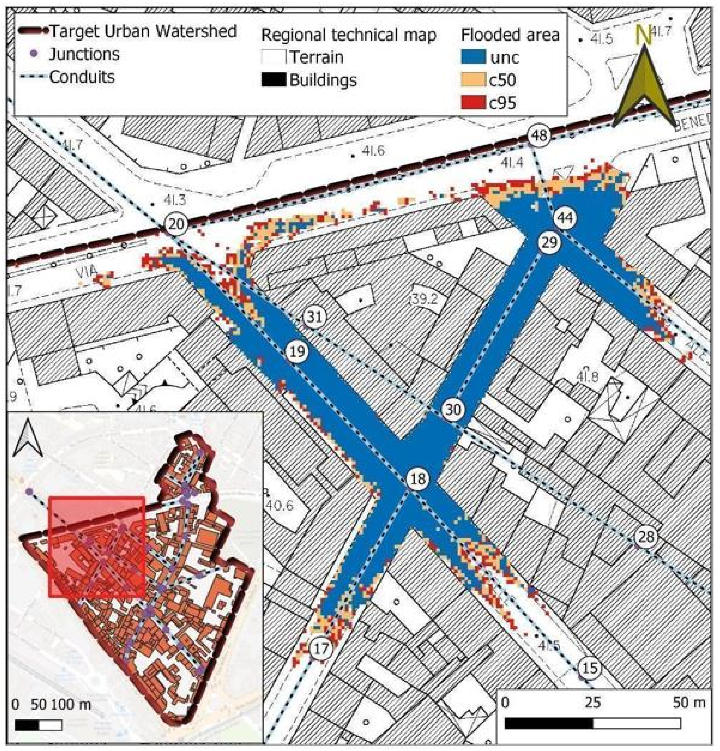
The comparison of the different flooded area delineations for the 20 year design event with 15 min duration can be seen in Figure 11. In the figure, the flooded area of the uncorrected scenario is in blue, the flooded area of the correction with the median value is in orange and the flooded area with the correction of the 95th percentile is in red.
The comparison between the flooded areas in Figure 11 displays that there is not a large difference between the corrected and the uncorrected design events. The not evident disparity between flood-prone areas is related to the marked sunken morphology of the urban watershed (see Figure 3), in which higher water depths do not reflect an outstanding wider flooded area.
5. Conclusions
The temporal aggregation of rainfall data plays a decisive role in estimating the annual maxima in the various durations, especially for the shorter ones. Over time, the data aggregation time may be subjected to changes as each hydrological service can arbitrarily choose how to process the raw data obtained from the instruments. In Tuscany, the aggregation time of the rainfall data changed over time and then stabilized at 15 min at the end of the 1990s and this has led to a loss of information regarding the maxima in the short durations. The errors in the underestimation of the annual maxima are acceptable for the maxima in the duration of 1 h or larger. Therefore, no implications on the design phase of the river basin with a time of concentration of more than 1 h can be detected. Thus, in these cases, the correction of the rainfall time series is negligible. Conversely, the errors that are committed using a temporal aggregation of 15 min can significantly impact the design phase of a new sewer system or underestimate the pluvial flood hazard in urban watersheds. For this reason, it would be important to decrease the temporal aggregation of rainfall data to use all the information that the rain gauges network can provide, reducing the uncertainty in the estimation of the annual maxima.
Author Contributions
Conceptualization, M.L., P.T., T.P. and E.C.; methodology, M.L. and R.M.; software, M.L. and P.T.; validation, M.L.; formal analysis, M.L. and P.T.; data curation, M.L.; visualization, M.L. and P.T.; writing—original draft preparation, M.L., P.T. and T.P.; writing—review and editing, R.M. and E.C.; supervision, R.M. and E.C. All authors have read and agreed to the published version of the manuscript.
Funding
This research received no external funding.
Institutional Review Board Statement
Not applicable.
Informed Consent Statement
Not applicable.
Data Availability Statement
The data presented in this study are available on request from the corresponding author.
Conflicts of Interest
The authors declare no conflict of interest.
References
- Rosenzweig, B.R.; McPhillips, L.; Chang, H.; Cheng, C.; Welty, C.; Matsler, M.; Iwaniec, D.; Davidson, C.I. Pluvial flood risk and opportunities for resilience. WIREs Water 2018, 5, e1302. [Google Scholar] [CrossRef]
- Schmitt, T.G.; Scheid, C. Evaluation and communication of pluvial flood risks in urban areas. WIREs Water 2020, 7, e1401. [Google Scholar] [CrossRef] [Green Version]
- Willems, P.; Arnbjerg-Nielsen, K.; Olsson, J.; Nguyen, V.T.V. Climate change impact assessment on urban rainfall extremes and urban drainage: Methods and shortcomings. Atmos. Res. 2012, 103, 106–118. [Google Scholar] [CrossRef]
- Masson, V.; Lemonsu, A.; Hidalgo, J.; Voogt, J. Urban climates and climate change. Annu. Rev. Environ. Resour. 2020, 45, 411–444. [Google Scholar] [CrossRef]
- Kourtis, I.M.; Tsihrintzis, V.A. Adaptation of urban drainage networks to climate change: A review. Sci. Total Environ. 2021, 771, 145431. [Google Scholar] [CrossRef]
- Schanze, J. Pluvial flood risk management: An evolving and specific field: Editorial. J. Flood Risk Manag. 2018, 11, 227–229. [Google Scholar] [CrossRef]
- Falconer, R.H.; Cobby, D.; Smyth, P.; Astle, G.; Dent, J.; Golding, B. Pluvial flooding: New approaches in flood warning, mapping and risk management. J. Flood Risk Manag. 2009, 2, 198–208. [Google Scholar] [CrossRef]
- Zhou, Q.; Mikkelsen, P.S.; Halsnæs, K.; Arnbjerg-Nielsen, K. Framework for economic pluvial flood risk assessment considering climate change effects and adaptation benefits. J. Hydrol. 2012, 414–415, 539–549. [Google Scholar] [CrossRef]
- Szewrański, S.; Chruściński, J.; Kazak, J.; Świąder, M.; Tokarczyk-Dorociak, K.; Żmuda, R. Pluvial flood risk assessment tool (PFRA) for rainwater management and adaptation to climate change in newly urbanised areas. Water 2018, 10, 386. [Google Scholar] [CrossRef] [Green Version]
- El-Zein, A.; Ahmed, T.; Tonmoy, F. Geophysical and social vulnerability to floods at municipal scale under climate change: The case of an inner-city suburb of Sydney. Ecol. Indic. 2021, 121, 106988. [Google Scholar] [CrossRef]
- Apel, H.; Trepat, O.M.; Hung, N.N.; Chinh, D.T.; Merz, B.; Dung, N.V. Combined fluvial and pluvial urban flood hazard analysis: Concept development and application to Can Tho City, Mekong Delta, Vietnam. Nat. Hazards Earth Syst. Sci. 2016, 16, 941–961. [Google Scholar] [CrossRef] [Green Version]
- Wang, Y.; Sebastian, A. Empirical numerical simulation of precipitation events for pluvial flood management. In Proceedings of the Geo-Extreme 2021, Savannah, GA, USA, 7–10 November 2021; American Society of Civil Engineers: Reston, VA, USA; pp. 21–29. [Google Scholar]
- Bulti, D.T.; Abebe, B.G. A review of flood modeling methods for urban pluvial flood application. Model. Earth Syst. Environ. 2020, 6, 1293–1302. [Google Scholar] [CrossRef]
- Simões, N.; Ochoa-Rodríguez, S.; Wang, L.-P.; Pina, R.; Marques, A.; Onof, C.; Leitão, J. Stochastic urban pluvial flood hazard maps based upon a spatial-temporal rainfall generator. Water 2015, 7, 3396–3406. [Google Scholar] [CrossRef]
- Sun, S.; Djordjević, S.; Khu, S.-T. A general framework for flood risk-based storm sewer network design. Urban Water J. 2011, 8, 13–27. [Google Scholar] [CrossRef]
- Di Salvo, C.; Ciotoli, G.; Pennica, F.; Cavinato, G.P. Pluvial flood hazard in the city of Rome (Italy). J. Maps 2017, 13, 545–553. [Google Scholar] [CrossRef] [Green Version]
- Guerreiro, S.; Glenis, V.; Dawson, R.; Kilsby, C. Pluvial flooding in European Cities—A continental approach to urban flood modelling. Water 2017, 9, 296. [Google Scholar] [CrossRef] [Green Version]
- Pregnolato, M.; Ford, A.; Glenis, V.; Wilkinson, S.; Dawson, R. Impact of climate change on disruption to urban transport networks from pluvial flooding. J. Infrastruct. Syst. 2017, 23, 04017015. [Google Scholar] [CrossRef] [Green Version]
- Hnilica, J.; Slámová, R.; Šípek, V.; Tesař, M. Precipitation extremes derived from temporally aggregated time series and the efficiency of their correction. Hydrol. Sci. J. 2021, 66, 2249–2257. [Google Scholar] [CrossRef]
- Morbidelli, R.; Saltalippi, C.; Dari, J.; Flammini, A. A review on rainfall data resolution and its role in the hydrological practice. Water 2021, 13, 1012. [Google Scholar] [CrossRef]
- Morbidelli, R.; Saltalippi, C.; Flammini, A.; Cifrodelli, M.; Picciafuoco, T.; Corradini, C.; Casas-Castillo, M.C.; Fowler, H.J.; Wilkinson, S.M. Effect of temporal aggregation on the estimate of annual maximum rainfall depths for the design of hydraulic infrastructure systems. J. Hydrol. 2017, 554, 710–720. [Google Scholar] [CrossRef] [Green Version]
- Young, C.B.; McEnroe, B.M. Sampling adjustment factors for rainfall recorded at fixed time intervals. J. Hydrol. Eng. 2003, 8, 294–296. [Google Scholar] [CrossRef]
- Yoo, C.; Jun, C.; Park, C. Effect of rainfall temporal distribution on the conversion factor to convert the fixed-interval into true-interval rainfall. J. Hydrol. Eng. 2015, 20, 04015018. [Google Scholar] [CrossRef]
- Morbidelli, R.; García-Marín, A.P.; Mamun, A.A.; Atiqur, R.M.; Ayuso-Muñoz, J.L.; Taouti, M.B.; Baranowski, P.; Bellocchi, G.; Sangüesa-Pool, C.; Bennett, B.; et al. The history of rainfall data time-resolution in a wide variety of geographical areas. J. Hydrol. 2020, 590, 125258. [Google Scholar] [CrossRef]
- Giannelli, D. Application of Sustainable Urban Drainage Systems for the Mitigation of the Pluvial Flood Risk in the Municipality of Florence. Master’s Thesis, University of Florence, Florence, Italy, 2020. [Google Scholar]
- Rossman, L.A. Storm Water Management Model User’s Manual Version 5.1; EPA/600/R-14/413b; National Risk Management Research Laboratory, Office of Research and Development, U.S. Environmental Protection Agency: Cincinnati, OH, USA, 2015. [Google Scholar]
Figure 1.
Temporal aggregation of rainfall in the Tuscany Region showed by the annual maxima series published by the Hydrological Regional Service (source: http://www.sir.toscana.it/, access on 11 November 2021).
Figure 1.
Temporal aggregation of rainfall in the Tuscany Region showed by the annual maxima series published by the Hydrological Regional Service (source: http://www.sir.toscana.it/, access on 11 November 2021).

Figure 2.
The geographical location of the Tuscany Region. Enlargement: spatial location of the rain gauge dataset used in this study.
Figure 2.
The geographical location of the Tuscany Region. Enlargement: spatial location of the rain gauge dataset used in this study.

Figure 3.
The geographical location of the study area. Enlargement: perimeter, topography and urban arrangement within the Target Urban Watershed—TUW.
Figure 3.
The geographical location of the study area. Enlargement: perimeter, topography and urban arrangement within the Target Urban Watershed—TUW.

Figure 4.
Photographic records and their locations of the last three intense rainstorms within the TUW.
Figure 4.
Photographic records and their locations of the last three intense rainstorms within the TUW.

Figure 5.
Aggregation of the time series for the annual maxima estimation with the generated time series, and the observed one, . In the figure, the maximum in the duration d of 1 h is estimated with three time of aggregations ta of 15 min, 30 min and 1 h.
Figure 5.
Aggregation of the time series for the annual maxima estimation with the generated time series, and the observed one, . In the figure, the maximum in the duration d of 1 h is estimated with three time of aggregations ta of 15 min, 30 min and 1 h.

Figure 6.
Annual Maxima Series (AMS) of Firenze Università rain gauge for the 4 considered durations.
Figure 6.
Annual Maxima Series (AMS) of Firenze Università rain gauge for the 4 considered durations.

Figure 7.
Sewer network within the Target Urban Watershed—TUW. The numbers represent the univocal name attributed to each junction (manholes).
Figure 7.
Sewer network within the Target Urban Watershed—TUW. The numbers represent the univocal name attributed to each junction (manholes).

Figure 8.
Comparison between the relation obtained by Morbidelli et al. [21], blue dashed line, in the Umbria Region (Italy) and the proposed functions of this study for the Tuscany Region: in orange, the correction associated at the median values of the error; in red, the correction associate at the 95th percentile.

Figure 9.
Design rainfall obtained by fitting the Generalized Extreme Value (GEV) on the annual maxima series (AMS) for the duration of 15, 45 and 60 min and with the Gamma distribution for 30 min duration. In blue, the probability distribution for the observed and uncorrected series, in orange, the correction corresponding to the 50th percentile, and in red, the correction corresponding to the 95th percentile. Return periods are expressed in years.

Figure 10.
Total Flood Volume (TFV) flowing out from the surcharged nodes. The symbols are used to distinguish the outcomes of the different scenarios: blue dots for uncorrected design rainfalls, orange squares for the design events corrected with EA50 and red triangles for the design events corrected with the EA95. Return periods are expressed in years.

Figure 11.
Comparison between the flooded areas obtained simulating an event with a duration of 15 min and return period of 20 years. The flooded area of the uncorrected scenario is in blue, the flooded area of the correction with the median value (c50) is in orange and the flooded area with the correction of the 95th percentile (c95) is in red.


Table 1.
Flooded areas [m2] for the different event durations and intensity corrections.
| Duration | Uncorrected | c50 | c95 |
|---|---|---|---|
| 15 min | 3848 | 4059 (16.5%) 1 | 4487 (28.79%) 1 |
| 30 min | 4224 | 4788 (13.35%) 1 | 4788 (13.35%) 1 |
| 45 min | 6162 | 6464 (4.84%) 1 | 6460 (4.84%) 1 |
| 60 min | 6883 | 7197 (4.56%) 1 | 7197 (4.56%) 1 |
1 Increment with respect to the uncorrected design event.
Publisher’s Note: MDPI stays neutral with regard to jurisdictional claims in published maps and institutional affiliations. |
© 2022 by the authors. Licensee MDPI, Basel, Switzerland. This article is an open access article distributed under the terms and conditions of the Creative Commons Attribution (CC BY) license (https://creativecommons.org/licenses/by/4.0/).
Share and Cite
MDPI and ACS Style
Lompi, M.; Tamagnone, P.; Pacetti, T.; Morbidelli, R.; Caporali, E. Impacts of Rainfall Data Aggregation Time on Pluvial Flood Hazard in Urban Watersheds. Water 2022, 14, 544. https://doi.org/10.3390/w14040544
AMA Style
Lompi M, Tamagnone P, Pacetti T, Morbidelli R, Caporali E. Impacts of Rainfall Data Aggregation Time on Pluvial Flood Hazard in Urban Watersheds. Water. 2022; 14(4):544. https://doi.org/10.3390/w14040544
Chicago/Turabian StyleLompi, Marco, Paolo Tamagnone, Tommaso Pacetti, Renato Morbidelli, and Enrica Caporali. 2022. "Impacts of Rainfall Data Aggregation Time on Pluvial Flood Hazard in Urban Watersheds" Water 14, no. 4: 544. https://doi.org/10.3390/w14040544
Note that from the first issue of 2016, this journal uses article numbers instead of page numbers. See further details here.