
Identification of Groundwater Radon Precursory Anomalies by Critical Slowing down Theory: A Case Study in Yunnan Region, Southwest China

1
School of Water Resources and Environment, China University of Geosciences, Beijing 100083, China
2
State Key Laboratory of Biogeology and Environmental Geology & MOE Key Laboratory of Groundwater Circulation and Environment Evolution, China University of Geosciences, Beijing 100083, China
3
Yunnan Earthquake Agency, Kunming 650225, China
*
Author to whom correspondence should be addressed.
Water 2022, 14(4), 541; https://doi.org/10.3390/w14040541
Submission received: 19 December 2021
/
Revised: 29 January 2022
/
Accepted: 7 February 2022
/
Published: 11 February 2022
(This article belongs to the Special Issue Earthquakes and Groundwater)
Abstract
:In this study, we use the critical slowing down (CSD) theory to identify the precursory anomalies of groundwater radon based on the 1000-day continuous data from 8 monitoring stations in Yunnan Province, China during the seismically active period of 1993–1996. The low-frequency and high-frequency information were extracted from raw groundwater radon data to calculate their one-step lag autocorrelation (AR-1) and variance, respectively, in order to identify the precursory anomalies. The results show that the anomaly characteristics can be divided into three categories: sudden jump anomalies, persistent anomalies, and fluctuation anomalies. The highest average seismic recognition rate is 72.78%, based on the high-frequency information’s autocorrelation, while the lowest is 45.08%, based on the low-frequency information’s variance. The crustal activity and the change in hydrogeological conditions are possibly the main factors influencing groundwater radon anomalies in the selected period in the study area. There is a positive correlation between the anomaly occurrence time and epicentral distance when epicentral distance is less than 300 km, which may be related to the seismogenic modes and hydrogeological conditions. This study provides a reference for identifying groundwater radon anomalies before earthquakes by mathematical methods.
1. Introduction
Earthquake disasters are important global issues concerning the development of human society, which can often be highly destructive due to the lack of early warning systems [1]. The geochemistry anomalies related to earthquakes are important research directions in the search for earthquake precursors with potential use in earthquake prediction [2]. With the improvement in the monitoring system, radon, which is considered as one of the key indicators of the geochemistry, has increasingly attracted the attention of researchers [3,4,5]. Radon is generated by the decay of 238U in rock and soil in the subsurface environment, and therefore remains in the soil or dissolves in groundwater. There are many published studies on the relationship between radon and earthquakes, suggesting that radon has the potential to be a good indicator of the precursory process [6].
It was first proposed in 1927 that radon anomalies in groundwater were related to earthquakes, but it was not until 30 years later that people collected accurate data showing the change in radon concentrations in groundwater before earthquakes [7,8]. The temperature, precipitation, and other meteorological factors can cause the seasonal variation in groundwater radon concentrations, but its anomalies may also be related to the change in tectonic stress [7,9]. Although it has become a consensus that radon anomalies could be related to earthquakes, it is generally very difficult to identify anomalies because radon concentration variations often show the characteristics of nonlinear dynamic fluctuations. Therefore, it is very necessary to find effective identification methods. The traditional statistical methods, to a certain degree, are subjective and inaccurate. Some data mining methods, such as machine learning and artificial neural networks, have been used recently and have made a few achievements [7,9,10,11].
Faced with the complexity of crustal movements, many scholars began to perform systematic statistical analysis [12,13]. In 1989, Bak [14] proposed the “self-organized criticality (SOC) phenomenon” and classified earthquakes as this phenomenon, which attracted seismic researchers’ attention to the precursor analysis of the critical threshold of complex dynamic systems [15,16]. With the in-depth study of complex systems in medicine, finance, ecology and other fields [17,18,19], scholars have found that many complex systems have critical points, before and after which the state of the system will change; the critical point is also called an “avalanche” in SOC phenomena [20]. Accordingly, how to identify the critical point has become the key issue in complex systems research.
The critical slowing down (CSD) theory has been widely used to indicate the critical point of complex systems, such as the critical state’s identification in clinical medicine, biological systems and climate change, etc. [21,22,23]. The CSD is a phenomenon before the tipping point, which is where a complex system shifts abruptly from a state to another state [24]. For earthquakes, the high stress state before a large earthquake is considered as before the critical point, and the stress release after the earthquake is after the critical point, so the earthquake can be regarded as the critical point. Before the earthquake, the fluctuation amplitude of the corresponding observation value increases and the recovery speed slows down until the occurrence of the earthquake. Numerous studies have found indicators that can reflect the CSD effectively [25]. Some scholars have also tried to apply this theory to the precursory anomaly identification in groundwater radon, and revealed that the CSD theory showed promise in dealing with the anomalous variations in groundwater radon and confirming the existence of critical slowing effects before earthquakes, which also provides an important reference for earthquake precursor identification [26,27,28,29]. In this study, the CSD theory is employed to identify the precursory anomalies in groundwater radon based on the 1000-day continuous data from 8 monitoring stations in Yunnan Province, China during the seismically active period of 1993–1996, which may provide ideas for the related research of identifying precursory anomalies in groundwater.
2. Geological and Hydrogeological Settings
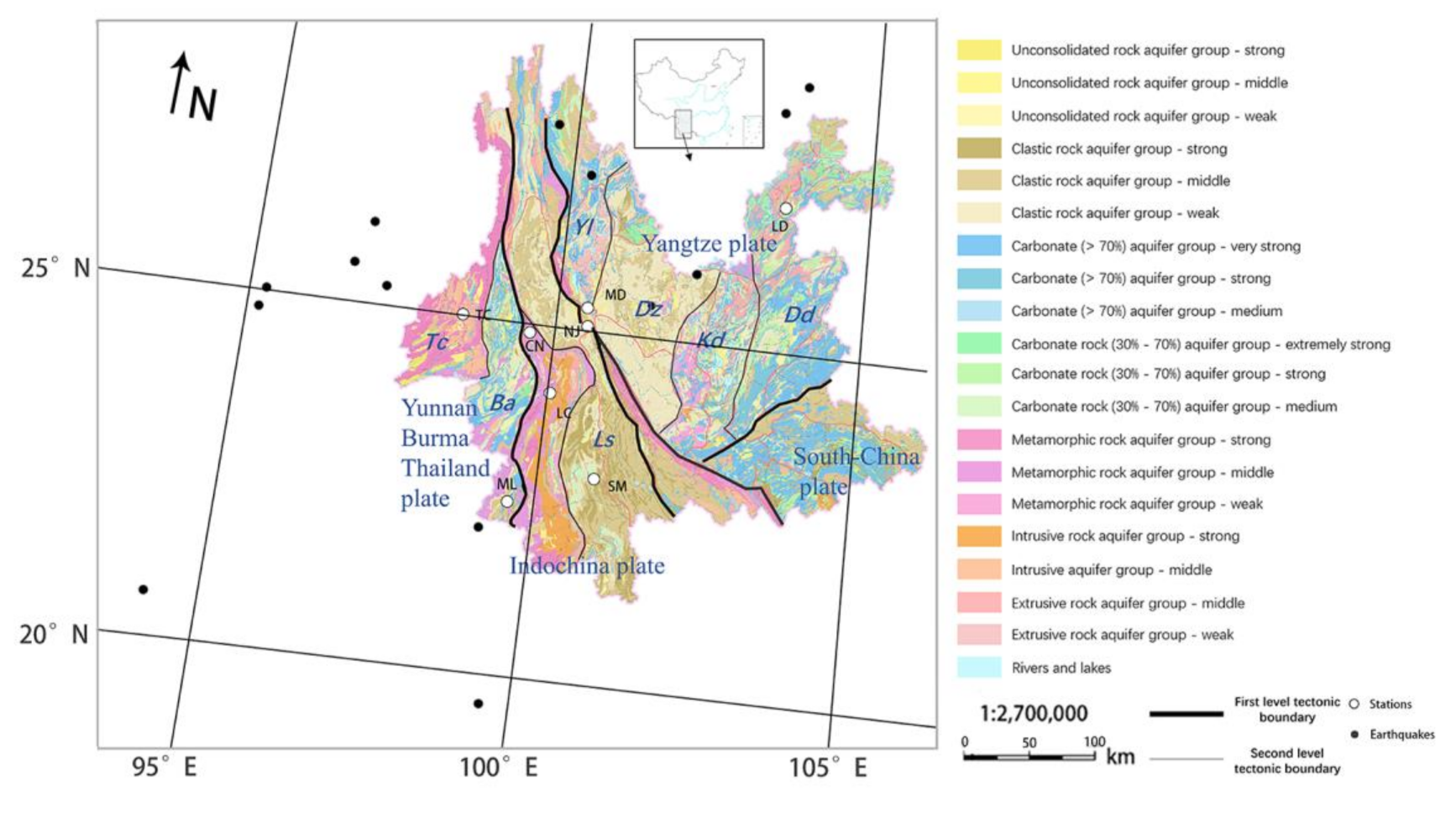
The eight monitoring stations are located in the west and north of the Yunnan region, Southwest China. The region is in the southeastern margin of the Qinghai-Tibet Plateau, and the edge zone of interaction between the Eurasian plate and the Indian plate (Figure 1). As one of the tectonically active regions, the Yunnan region is characterized by the high-frequency, large magnitude and wide distribution of earthquake activities [30,31]. According to the earthquake catalogue of the National Earthquake Information Center (NEIC), more than 289 earthquakes with M ≥ 5 occurred in Yunnan region in the 20th century, including 13 earthquakes with M ≥ 7 [9].
From west to east, there are three large-scale faults in the region, i.e., the Lancangjiang fault, the Jinshajiang-Red River fault and the Xiaojiang fault, and there are four main sub-plates, i.e., the Yunnan-Burma-Thailand (YBT) plate, the Indochina plate, the Yangtze plate and the South-China plate.
As shown in Figure 1, in the YBT plate, the Tengchong block is mainly metamorphic rock aquifer, and the Baoshan block is mainly carbonate rock aquifer; in the Indochina plate, the Lanping-Simao back arc basin is mainly clastic rock aquifer, and the rest is metamorphic rock and magmatic rock aquifers; the Yangtze plate has complex fold structures and various aquifers. Among them, the central Yunnan depression is mainly composed of loose sedimentary aquifers and clastic rock aquifers, and the aquifers of other plots are mainly carbonate rock aquifers, mixed with metamorphic rock aquifers and magmatic rock aquifers. The South China plate is mainly carbonate rock aquifer in the center, and the boundary with the Yangtze plate is clastic rock aquifer (Figure 1).
3. Data Preprocessing
There were four seismic active periods in Yunnan region in the 20th century, and the last period started in 1988 and ended in 1996 [31]. During that period, there were two earthquakes with magnitudes larger than 7, which were the Menglian earthquake (12 July 1995, Mw 7.2) and the Lijiang earthquake (3 February 1996, Mw 7.0). Therefore, we chose this region as the study area. We collected 1000 days of data (9 May 1993–3 February 1996), which is in the active period of earthquakes in the region where the eight monitoring wells were distributed. Groundwater samples were collected daily using a pre-vacuumed glass bottle and radon concentrations were measured on the same day using the FD-105K instrument (Shanghai Electronic Instrument Co., Ltd., Shangjai, China) based on the scintillation method. The locations of the monitoring wells are shown in Figure 1. The longitude and latitude of the stations are shown in Table 1.
We can calculate the possible occurrence range of earthquake precursors according to the empirical formula:
where is earthquake magnitude and is epicenter distance (km) [32]. The calculation results show that the precursory range of M 5.0 earthquake is 141.25 km and the range is more than 1000 km when the M is greater than 7.
Hauksson et al. put forward an empirical formula for water radon anomalies before earthquakes with M ≥ 5, as follows:
where is earthquake magnitude and is epicenter distance (km) [33]. The calculation results show that the precursory range of M 5.0 earthquake is 183 km and the range is more than 1246 km when the M is greater than 7.
Assuming that the precursory response is highly correlated with the co-seismic effect [9], the precursory range can be also estimated according to the formula [34]:
where is the energy density, is earthquake magnitude and is epicenter distance (km). Wang et al. indicated that the hydrological response in some areas is very sensitive, and the response to energy density may be as small as 10−4 J/m3 [35], so we selected earthquakes with seismic energy density greater than 10−4 J/m3 as earthquakes whose precursor may occur at the stations. When the energy density is 10−4 J/m3 and the magnitude is 5, the maximum epicenter distance is 256.8 km; when the magnitude is 7, it is greater than 2300 km.
Walia et al. summarized the empirical formula for the occurrence range of radon anomalies before earthquakes and pointed out that the range in radon anomalies before earthquakes can be far greater than the calculation results of the empirical formula [36]. Therefore, we only took the above results as references. By investigation of the occurrence of earthquakes in the study period in the study area, we finally selected the data of earthquakes with magnitude greater than M 5.0 within the farthest 500 km of the most marginal stations from 9 May 1993 to 3 February 1996, according to the earthquake catalogue of the NEIC, for calculation. We only selected earthquakes with the largest magnitude among multiple earthquakes occurring in a short time in the same area. The earthquakes finally selected are shown in Table 2.
4. Method
4.1. Wavelet Transform (WT)
We note that in previous studies using the CSD theory, some studies chose not to carry out data preprocessing, and some used filters to eliminate the trend information of time series and only retained the residual, i.e., random fluctuations, to observe the potential critical point warning of complex systems. However, we note that when the observation period is long, there may also be effective information in the trend information, no matter what filtering method is selected; thus, only retaining the residual may cause a loss of this effective information. In this study, we used the wavelet decomposition (WD) as the filtering method to split the time series of radon concentration into trend information (low-frequency information) and residual (high-frequency information), and further analyzed and compared them, respectively.
Wavelet analysis, which is composed of wavelet basis functions, is a method of signal analysis in both the time domain and the frequency domain. With the in-depth exploration of data analysis in recent years, the mathematical methods based on wavelet theory play an important role in extracting data information [7,9]. Compared with Fourier transforms, wavelet analysis methods including continuous wavelet transforms (CWTs) and discrete wavelet transforms (DWTs) have better accuracy in local time and frequency domains. Therefore, it is widely used in image, signal and other fields for data analysis, denoising, signal contrasts, etc.
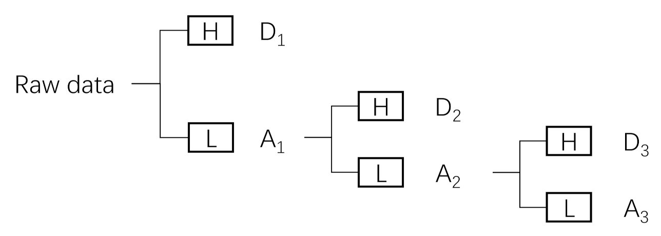
Wavelet decomposition (WD), as one of the methods of wavelet transforms, is based on the multi-resolution theory proposed by Malat [37]. It decomposes the original non-stationary signal into several detail coefficients and one approximation coefficient by using multi-resolution analysis, and the level of decomposition is the number of decomposition layers. The length of the signal is damaged every time, so it needs to be reconstructed by interpolation to obtain the high and low-frequency signals. Figure 2 is a schematic diagram of this process. By adjusting the number of decomposition layers, one can obtain the required high-frequency information (Residuals) and low-frequency information (Trend).
Wavelet coherence (WTC) is also a method of WT. It can effectively reveal the phase relationship between two time series. It is defined as follows [38]:
where is an operator, is a smoothing operator, is wavelet scale, and is the wavelet coherence of two time series, which resembles the traditional correlation coefficient. In this study, the statistical significance level of WTC is determined by Monte Carlo methods [39]. Edge effects caused by discontinuities at endpoints are evaluated by Cone of Influence (COI) [40].
4.2. CSD Theory
In 2009, Schaefer et al. proposed that critical slowing is related to three potential early warning indicators, namely disturbance recovery rate, autocorrelation and variance [24]. Vasilis et al. summarized the indicators that can indicate the critical slowing phenomenon, including autocorrelation at lag 1 (AR-1), return rate, variances, spectral density etc. [25]. For the autocorrelation and variance, they will increase rapidly when the CSD phenomenon occurs. The autocorrelation will tend to 1 and the variance will tend towards infinity. These early-warning signals are the result of CSD near the threshold value of the control parameter [24].
For the statistical variance and autocorrelation calculation of data, the following formula is used:
where is lag length. represents the ith data, is the mean, is the number of data points in the sample, is the standard deviation and is the variance.
5. Parameter Selection
To explore the possible residual anomalies and trend anomalies in groundwater radon, this study extracts the high frequency information and low frequency information from the continuous monitoring radon data through WD, and then calculates their autocorrelation and variance, respectively. In the process, there are three main parameters affecting the results, namely, the level of WD, window length (WL) and window lag step. In this paper, the lag step is set as 1, and then the two scenarios of fixed window length adjusting WD level and fixed WD level adjusting WL are analyzed respectively (See Supplementary Material for detailed analysis of parameter selection). The results show that:
- (1)
- The change in parameters has less influence on the variance but greater influence on AR-1. The results of AR-1 are complex and changeable, which may be because the calculation of AR-1 requires high sampling frequency data.
- (2)
- The influence of parameter changes on results derived from the high-frequency information is less than that from low frequency information. In the results of high-frequency information, the AR-1′s and variance’s anomalies under different WL and different levels of WD all appear at the same time point. This shows that the changes in parameter values have little effect on the high frequency information calculation results. However, the low frequency information calculation results vary greatly under different parameter values. With the increase in WL, the abnormal points of low frequency are delayed gradually; with the increase in level of WD, the resulting curve of low frequency gradually changes from fluctuation to stability until it approaches a straight line.
Considering that the influence of different parameters on the high-frequency-information calculation results is not obvious, while the low-frequency calculation results are regular, we chose moderate parameters, level 5 for WD and 10 days for WL.
6. Results
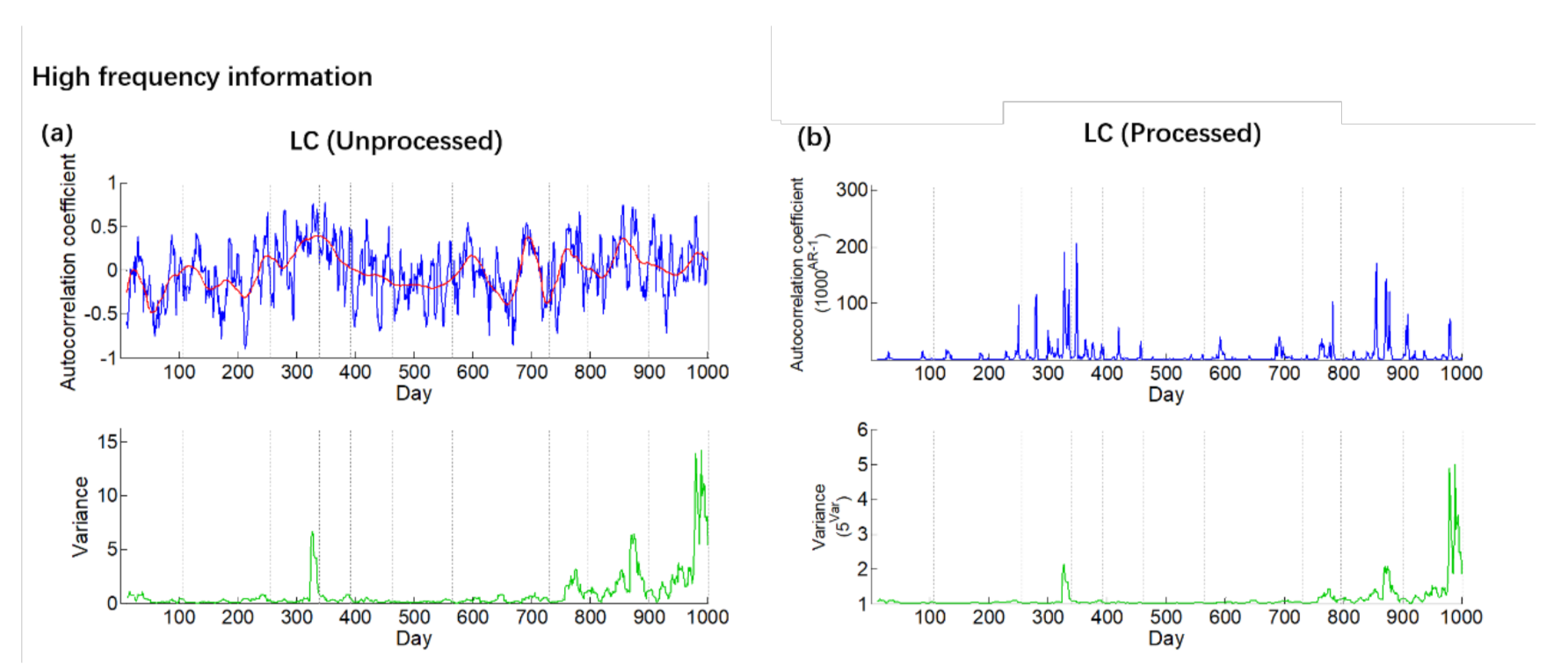
We computed the autocorrelation and variance of high-frequency information and low-frequency information data on groundwater radon for each monitoring well. Due to the calculation results fluctuating sharply, it is difficult to obtain effective information (Figure 3a, taking LC monitoring well as an example). According to CSD theory, the closer the recovery rate of the system is to 0, the closer the autocorrelation coefficient is to 1; that is, the more significant the CSD phenomenon is [21]. We transformed the original AR-1 values with a power function to enlarge the value in order to make the anomalous values more visible. For the variance, in order to facilitate observation, we chose to normalize it, and substituted it into the power function as well. The functions of AR-1 and variance substitution are:
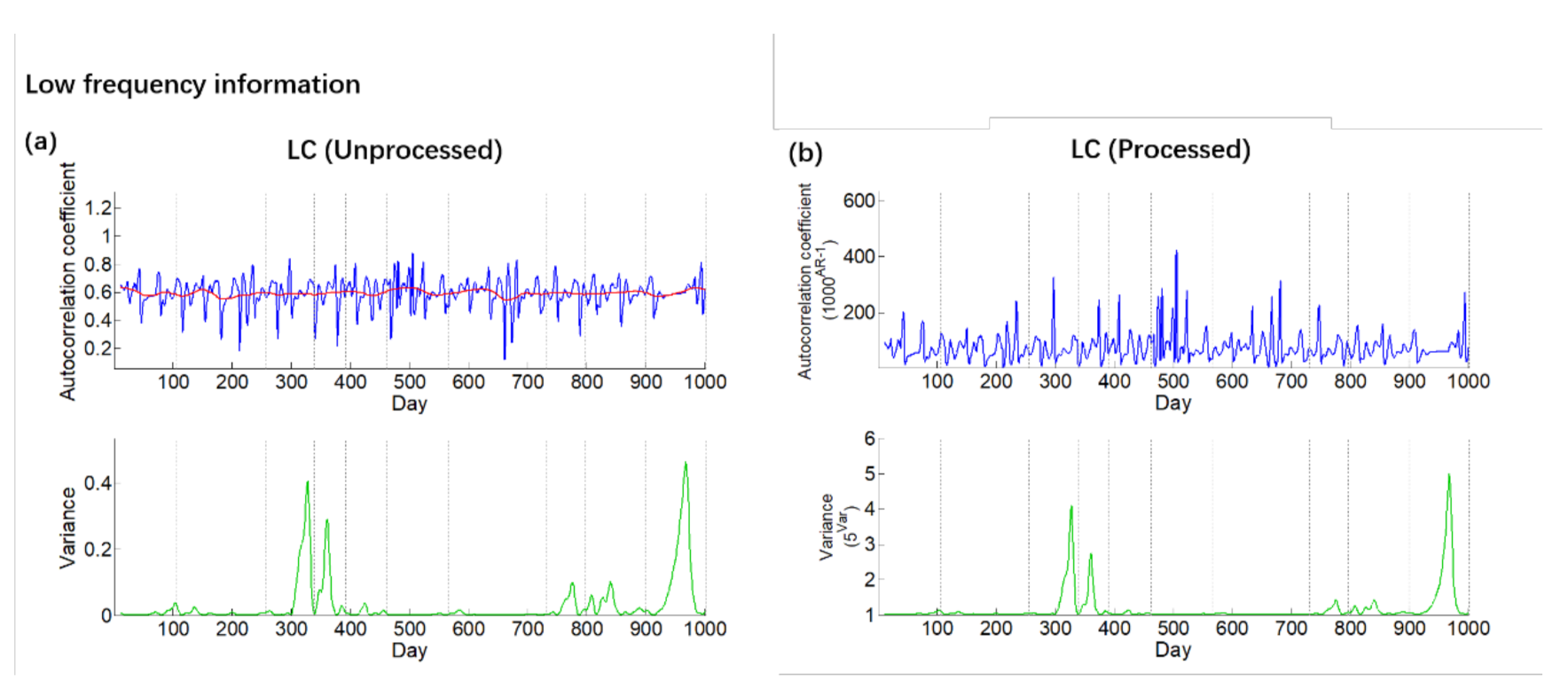
As shown in the Figure 3b, the uplift point of the AR-1 and of the variance is shown clearly after processing, and the peak points are basically consistent with Figure 3a. The similar situation can be seen in Figure 4a,b. Through such processing, we can distinguish the peak points and take them as the candidate anomalies in the groundwater radon data.
In this study, we conducted the above processing on the calculation results of all monitoring stations, and then we selected IQR (interquartile range) plus median as the anomaly standard to filter the anomaly values.
6.1. The Results of High-frequency Information (Residuals)
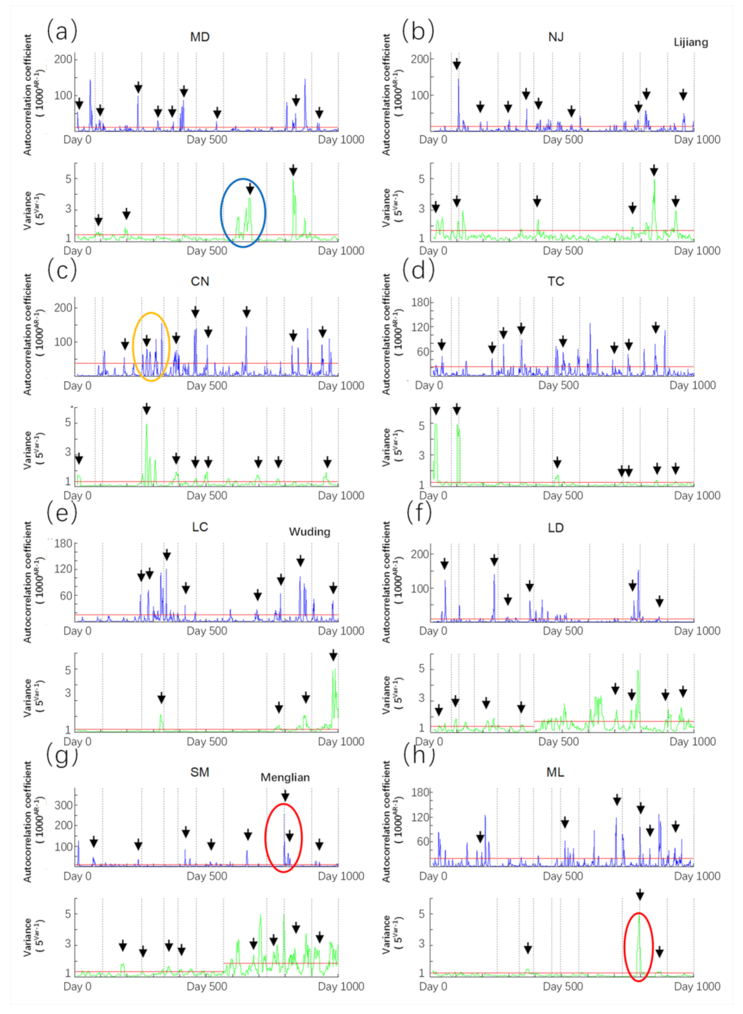
The calculation results of high-frequency information are shown in Figure 5. The anomaly characteristics can be divided into three categories: sudden jump anomalies, fluctuation anomalies and persistent anomalies. The sudden jump anomaly means an increase in value in a short time, with only one significant peak and duration less than 10 days (such as red circle in Figure 5g,h); the fluctuation anomaly is that it breaks through the anomaly threshold for many times in a short time, forming many peaks in a short time (such as yellow circle in Figure 5c); the persistent anomaly is one that remains above the anomaly threshold for more than 10 days (such as the blue circle in Figure 5a).
It is shown in Figure 5 that there are differences in the main anomaly characteristics of AR-1 at each station. In the stations of MD, LD and SM, there are mainly sudden jump anomalies (Figure 5a,f,g); Cn, TC, LC and ML are mainly fluctuation anomalies (Figure 5c–e,h); in the station of NJ, the three characteristic anomalies exist (Figure 5b). There are some persistent anomalies in AR-1, but the duration is short, the anomaly value is small, and the fluctuation is frequent, so it is difficult to strictly distinguish it from the other two anomaly characteristics. Generally speaking, the abnormal characteristics of AR-1 are mainly sudden jump anomalies and fluctuation anomalies.
The anomaly characteristics of variance are mainly sudden jump anomalies and persistent anomalies. The persistent anomalies in variance have obvious characteristics, long duration, and most peaks are obvious. Most of the sudden jump anomalies of variance are co-seismic anomalies with large values and significant characteristics. The fluctuation anomalies in most stations are not obvious, but the variance results of LD and SM show large fluctuations after an earthquake, forming a long-time-scale fluctuation anomaly (Figure 5f,g).
Some anomalies in AR-1 and the variance appeared synchronously in some wells. However, except for a few earthquakes, the synchronization of the two indexes in response to most earthquakes is poor. For example, the two indicators of LD, SM and ML have abnormal responses to earthquakes at the same time in the Menglian earthquake (day No. 800). The two indicators of LC are basically synchronized with the seismic response after the Wuding earthquake (day No. 700). In most cases, only one indicator responds to earthquakes. The number of anomalies of variance is less than that of AR-1.
The empirical formula for the relationship between the occurrence time of earthquakes and precursors is as follows:
where (km) is the epicenter distance, (days) is the number of days before the earthquake when the earthquake precursor appears, and is the earthquake magnitude [41]. According to the calculation, the maximum occurrence time of the precursor with less than 500 km epicenter distance is about 73 days before the earthquake.
We take the time between the occurrence of precursory anomalies at each station and that of the subsequent earthquakes as the number of abnormal days in advance. According to the CSD theory, the lifting point indicates that the complex system begins to enter the CSD state. However, in order to facilitate identification, we select the peak point as the abnormal point for the sudden jump and fluctuation anomalies, because the peak point and uplift point are very close. For the persistent anomaly with a long interval between the uplift point and the peak point, we still take the uplift point as the anomaly point. Considering the effect of the length of WL, we assume that the precursory anomaly point is the first peak point between the two earthquakes within 83 days (73 days plus 10 days) before the next earthquake. The results are shown in Table 3 and Table 4. We take the ratio of the number of earthquakes with pre-earthquake anomalies at the station to the number of earthquakes with seismic energy density ≥ 10−4 J/m3 as the recognition rate. The results show that the recognition rate of AR-1 in MD station is the highest, which is 81.82%; the variance recognition rate of LD station is the highest, which is 80%. The average recognition rate of AR-1 in 8 stations is 72.78%, which is greater than the 55.34% of the variance (Table 5).
6.2. The Results of Low-frequency Information (Trend)
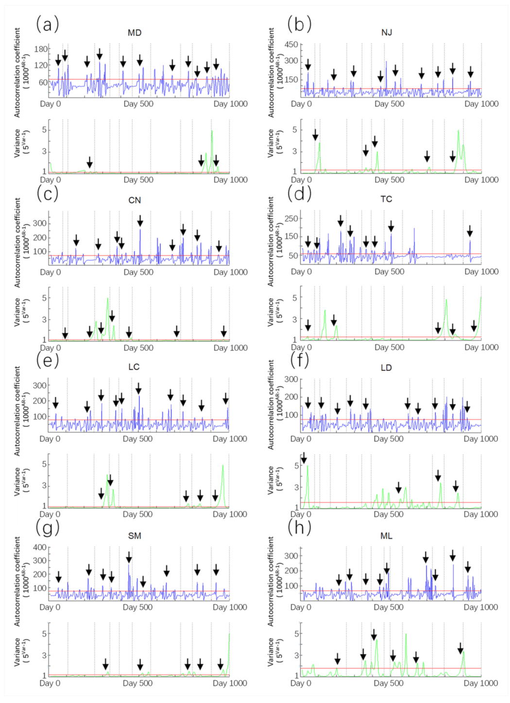
The calculated results from low-frequency information data of each station are shown in Figure 6. The results show that there are significant differences in the abnormal characteristics of low-frequency information AR-1 and variance. In the AR-1 results, the fluctuation anomaly is the main anomaly type, the sudden jump anomaly is the secondary anomaly type, and there is no persistent anomaly in the eight stations. In the variance results, persistent anomalies are the main anomaly feature. Compared with high-frequency information, the average value of low-frequency-information AR-1 is higher. The variance results show an obvious peak like protrusion, which is similar to the calculation results of high-frequency information, but they are smoother. The rising process of the variance curve can be clearly seen. There is a large interval between the date when the variance value breaks through the anomaly threshold (uplift point) and the date of the peak, showing obvious characteristics of persistent anomalies.
The peak of AR-1 results has less relationship with the peak of variance results. There is no co-seismic peak in AR-1 results, but the variance results in MD, NJ and ML stations have a co-seismic peak at the time of the Wuding earthquake. The variance anomaly in low-frequency information lasts longer, often breaks through the anomaly threshold some time before the earthquake, and finally reaches the peak before or a few days after the earthquake.
We selected the peak point of AR-1 results as the anomaly point, and the intersection of the variance curve and the anomaly standard line as the anomaly point (uplift point) for the variance results. The results are shown in Table 6 and Table 7. The AR-1 recognition rate of LC is the highest, which is 100%; ML has the highest variance recognition rate of 60%. The average recognition rate of low-frequency AR-1 is 88.24%, which is higher than that of high-frequency AR-1; the average recognition rate of variance is 45.08%, which is about 10% lower than that of high-frequency variance (Table 8).
Comparing the calculation results of high-frequency information with those of low-frequency information, it can be seen that the variance recognition rate of high-frequency information is higher, and the AR-1 recognition rate of low-frequency information is higher. For the same earthquake, the synchronization of variance response in high-frequency results and low-frequency results is higher than that of AR-1.
7. Discussion
7.1. Interfering Factors
Previous studies showed that radon anomalies are not only affected by tectonic activities, but also affected by meteorological conditions such as air temperature, air pressure and precipitation. [4,7,42,43,44,45,46]. In this study, we collected atmospheric pressure (PRS), air temperature (T) and precipitation (PR) data of each station, and the missing data was supplemented by the monitoring data of nearby stations. We calculate the wavelet coherence (WTC) of atmospheric pressure, temperature and precipitation on radon concentration, and calculate the correlation between pressure, temperature and precipitation and raw radon data, low-frequency data and high-frequency data.
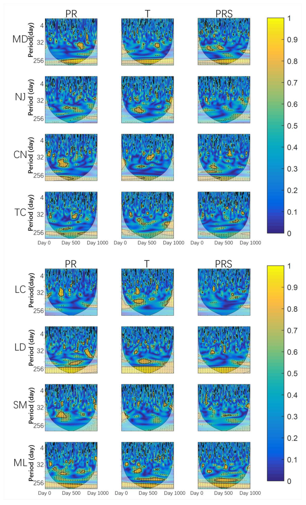
As shown in Figure 7, in the results of wavelet coherence in the whole observation time, the three WTC images of each station are similar. This may be due to the similar seasonal cycle period of air pressure, temperature and precipitation. Radon and air pressure, air temperature and precipitation of MD, CN, TC, LD and ML stations have coherence within the band of 1 year in the whole period; PRS, T and PR of CN and TC stations showed coherence with radon in some time periods. CN station showed correlation before September 1994 (about day No.500), and TC station showed a high coherence for a 1 year band in May 1993 to March 1994 and 1995 to 1996. The PRS, T and PR at NJ, LC and SM stations do not show correlation with radon within the band of 1 year. There was a correlation between radon and T and between radon and PR of ML station within the band of a half year in June 1994 to July 1995. For other bands, there are sporadic correlations in each station’s results, but the duration is short, mostly within 100 days.
In addition, we also calculated the correlation coefficients of air pressure, precipitation and temperature to the original radon data, high-frequency information data and low-frequency information data. The formula is as follows:
where is correlation coefficients, is the number of data, and mean the ith data of x and y respectively, and and mean the average value of x and y respectively. The calculation results are shown in Table 9. There are nine results for each station. For the correlation coefficient, less than 0.3 is considered as no correlation, and 0.3 to 0.8 is considered as a weak correlation [47]. The results of the correlation coefficient show that PRS, T and PR have no significant correlation with radon.
The calculation results for R at each station show that radon concentration has no certain correlation with PR, while it can be seen from WTC that except for LD and ML stations, radon and PR of other stations have correlation only for part of the time or no correlation, which is similar to the result for R. We speculate that this may be related to the well depth. For deep groundwater, the response of groundwater dynamics to the infiltration recharge of precipitation is delayed, and precipitation signals may be smoothed, resulting in that the correlation between the two cannot be identified.
According to Feng’s study [48], the increase in air pressure will make the degassing effect worse and reduce the radon concentration in water, but the influence of air pressure on radon concentration in deep groundwater is small. That may be why the relationship between air pressure and radon concentration is not obvious in our calculation results.
The formula for radon dissolution is as follows [49]:
where S is the solubility of radon and the T is the temperature. We can see that the increase in temperature will increase the solubility of radon, thus increasing the concentration of radon in water. However, there is no obvious correlation in R results, and there is even a negative correlation between temperature and radon concentration in NJ and MD.
According to the calculation results of WTC, meteorological factors have a certain impact (mainly periodic) on radon concentrations in water, which is consistent with the previous research conclusions. It is worth noting that in the results of WTC, there is a stable strong correlation (mainly periodic) between water radon concentration and meteorological factors in two stations (LD and ML); however, the calculation results of R show that there is no strong correlation between meteorological factors and water radon in eight stations. Overall, meteorological factors did not cause short-term radon concentration changes.
7.2. Possible Explanations for Different Anomaly Characteristics
In the results, we summarized three kinds of anomaly characteristics, namely sudden jump anomalies, fluctuation anomalies and persistent anomalies. Previous studies showed that radon concentrations in water are closely related to the state of the seismogenic system [4,5,50]. Therefore, if we regard the rock rupture as an “avalanche point” of the complex system of block motion on a micro level, the anomalies in AR-1 may indicate the micro fracturing process of rocks near the monitoring well. From the physical meaning of the index, the AR-1′s sudden jump anomaly indicates that the recovery speed of the system suddenly decreases and approaches the “avalanche point” in a certain moment within WL (10 days). Fluctuation anomalies in AR-1 mean that the state of the system changes sharply over a period of time. Persistent anomalies in AR-1 mean that the state of the system’s recovery speed keeps slowing down over a period, which is a typical sign of CSD in other studies. For variance, sudden jump anomalies mean that the sample data has changed greatly at a certain moment within 10 days. Fluctuation anomalies represent multiple numerical mutations with an interval of about 10 days over a period of time. Persistent anomalies indicate that the sample data are in a state of large fluctuation ranges for a period of time. The three types of anomaly characteristics may be caused by different water radon anomaly mechanisms.
Zhang et al. proposed that as an important carrier of radon migration, groundwater flow anomalies have an important impact on radon [7]. The precursory mechanism of water radon anomalies may be closely related to the change in permeability during earthquake preparation. In the process of earthquake preparation, the accumulation of stress and strain may cause changes in crustal permeability [51]. The continuous accumulation process constantly disrupts the mechanical balance between particles, moving each other, changes the porosity and groundwater flow, and finally leads to “avalanches” and forms new pore channels. In this process, the radon concentration in water changes continuously, which may provide an explanation for the persistent anomaly.
According to the theory of the “strong body earthquake-generating model” [52], when the crustal deformation process outside the nucleation area continues to develop, it may lead to frequent rock micro fractures for a period of time, resulting in frequent changes in hydrogeological conditions and radon concentrations, manifested by irregular and frequent fluctuations over a short time, forming fluctuation anomalies, until the rock mass in the nucleation area suddenly breaks when the pressure reaches the threshold, forming an earthquake. The frequent rock micro fracturing in this process may provide an explanation for the sudden jump anomalies and fluctuation anomalies.
In addition, the main anomaly characteristics in the results of different stations are different. Binda et al. revealed that the response of hydrogeochemistry to seismic activity is closely related to hydrogeological conditions. This indicates that different hydrogeological conditions may lead to different responses [53]. In the present study, in the high-frequency results of MD and LD, AR-1 mainly shows the sudden jump anomalies. MD is a thermal water well with a shallow well depth and LD is a spring. In terms of lithology, MD and LD are in sedimentary rocks with significant karstification that may lead to a good hydraulic connection among aquifers. It is possible that the mixing between shallow groundwater and deep fluid or gas will occur occasionally during earthquake preparation, thus causing a sudden jump anomaly. In contrast, high-frequency results of AR-1 in TC and LC mainly presented with fluctuation anomalies. The formation lithologies of TC and LC are magmatic rocks, and the well depth is relatively deep and groundwater is fissure water. We speculate that the change in groundwater radon concentration in the wells mostly result from the release of rock micro fracturing caused by crustal stress due to the poor hydraulic connection and relatively stable conditions. The relatively stable conditions may amplify the slight fluctuations of radon concentration in groundwater, making fluctuation anomalies the main anomaly feature of AR-1 at these two stations. On the whole, different hydrogeological conditions, along with regional stress and strain changes, could result in different responses of aquifers and the associated different anomalies in water radon concentration at each station, requiring further study.
7.3. Temporal and Spatial Characteristics of Radon Anomalies
7.3.1. Relationship between Epicenter Distance and Anomaly Occurrence Time at Each Station
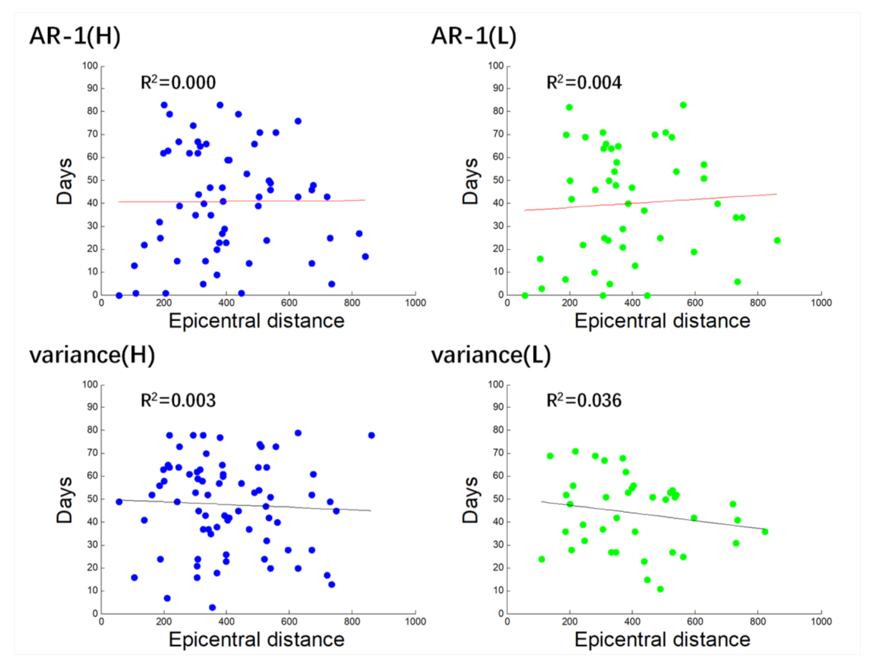
Some previous studies suggest that there may be a spatio-temporal relationship between the occurrence of earthquakes and precursors. In the present study, we conducted the statistical analyses on the occurrence time of each earthquake and earthquake precursory anomalies, and calculated the time of precursory anomalies ahead of the earthquakes (Table 3, Table 4, Table 6 and Table 7). Then, we plotted the diagram of precursory time and epicentral distance to investigate the possible relationship between them. When we take the single station as the research object, most R2 of the results are less than 0.1, reflecting that there is no certain linear correlation between the precursory time and epicentral distance. Considering that there may be too little data at a single station that may result in a great uncertainty of results, we drew a scatter diagram with all the stations’ data (Figure 8). Whether it is high-frequency or low-frequency data, or AR-1 or variance, the data points in the figures are randomly and irregularly distributed. R2 of the correlation showed in the figures is far less than 0.1, indicating that there is almost no linear relationship between precursory time and epicentral distance.
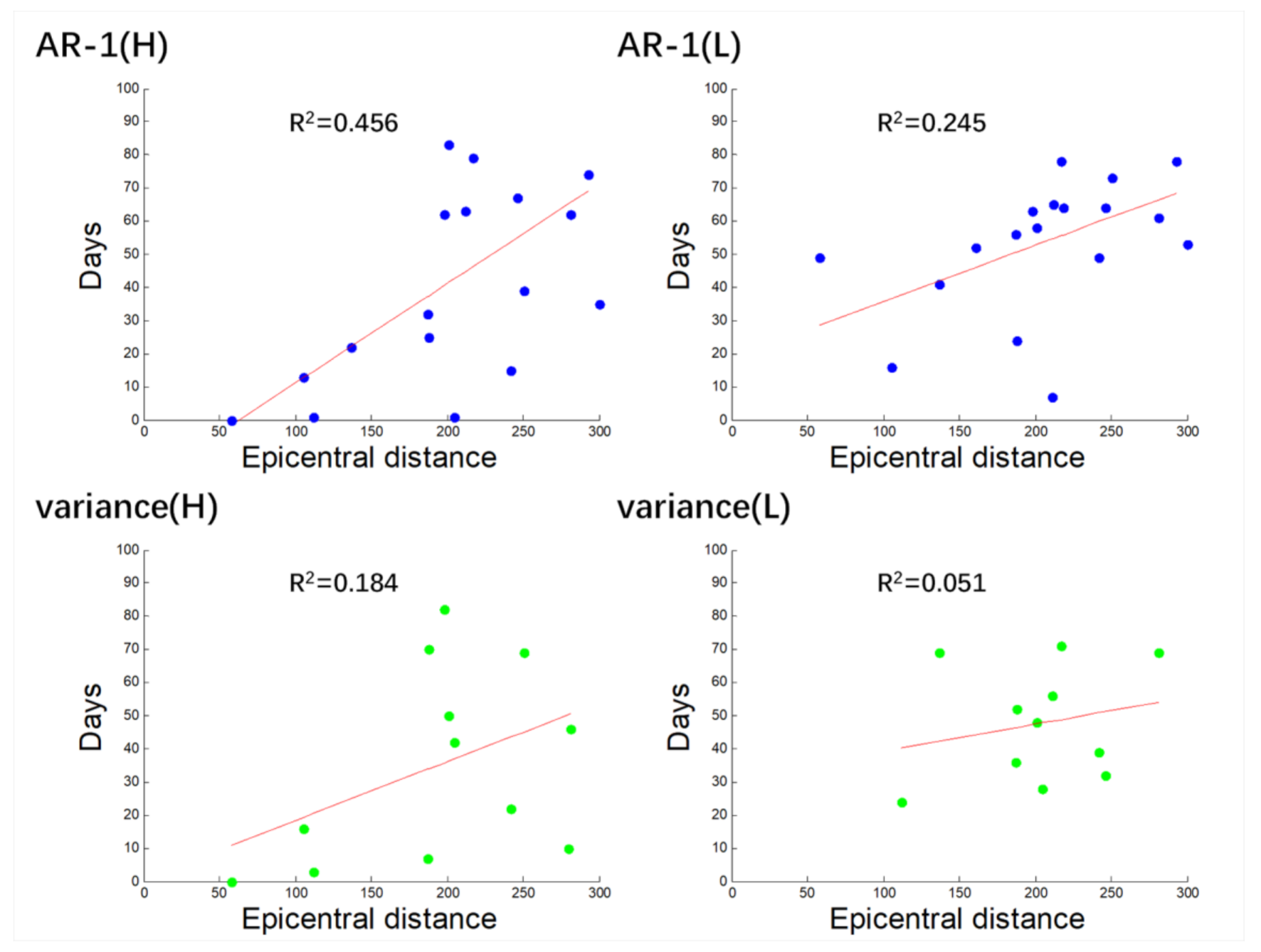
When we chose the earthquakes with the epicentral distance less than 300 km, the associated calculation results showed that the R2 of correlation between the epicentral distance and precursory time of variance (L), AR-1 (L) and variance (H) ranges from 0.051 to 0.245 (Figure 9), indicating that there may be a very weak or no positive correlation. However, the R2 of the epicentral distance and precursory time of AR-1 (H) is close to 0.5, showing an obvious positive correlation. This may indicate that within 300 km, the larger the epicenter distance is, the earlier the occurrence time of water radon precursor anomalies. This conclusion is consistent with that of some previous studies.
In some areas, there is also a positive correlation between the time of radon anomalies and the epicentral distance. According to the calculation results of the previous empirical formula (1), the seismogenic range of the M 5.7 earthquake is about 300 km. Considering that there is a high frequency of earthquakes with M 5–6 in the study area, we speculate that this phenomenon may be closely related to the earthquake preparation process. According to Mei’s “strong body earthquake generating model”, when the earthquake begins to prepare, a large number of small fractures will appear in the edge area with low fracturing strength, which leads to the earliest abnormal radon concentrations in peripheral groundwater. With the accumulation of stress, the fracturing gradually migrates to the epicenter, finally forming a phenomenon that the abnormal time is proportional to the epicenter distance. This may provide an explanation for such correlations.
7.3.2. Relationship between Epicentral Distance and Anomaly Time of Three Large Earthquakes
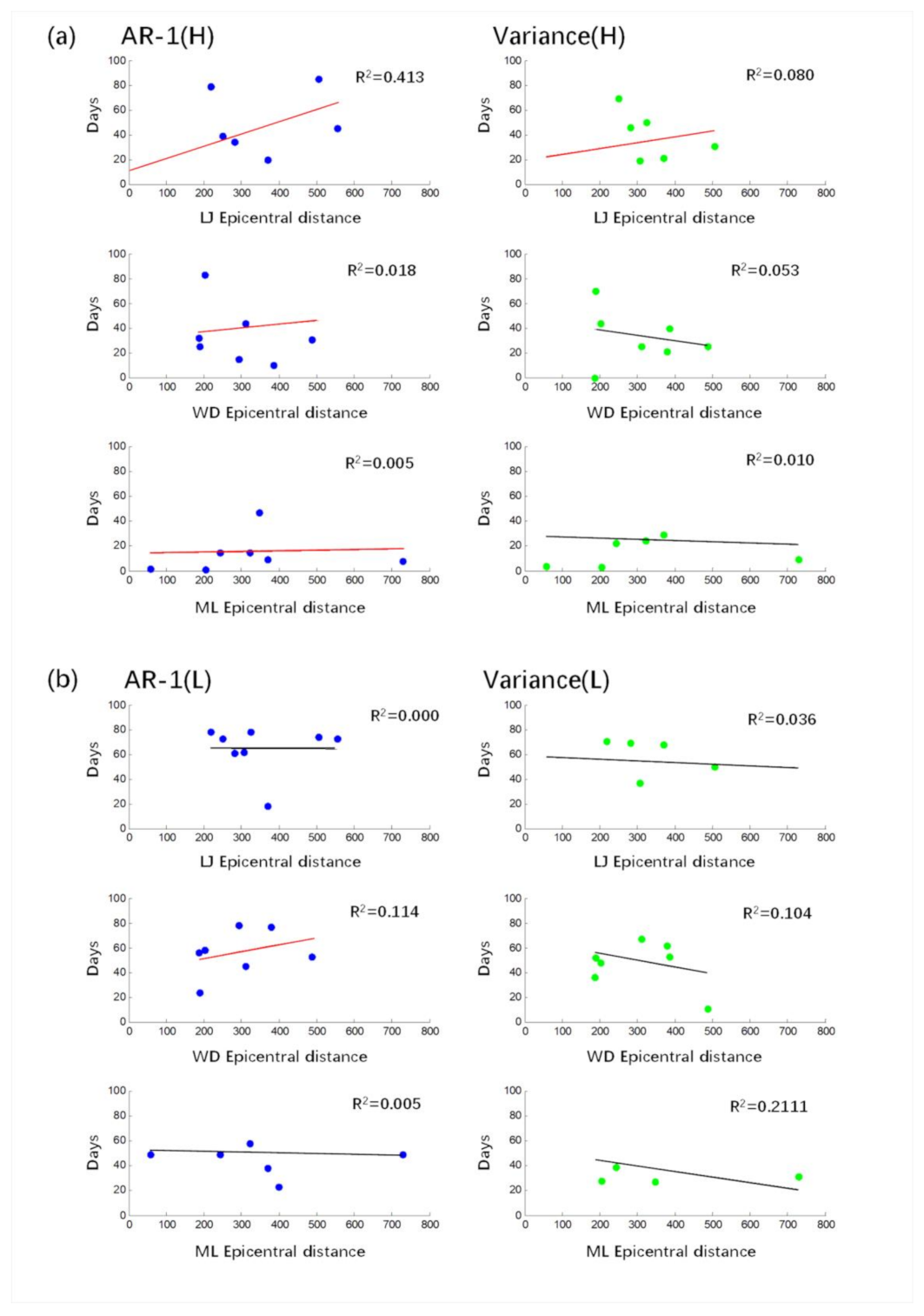
Taking the Lijiang, Wuding and Menglian earthquakes as the research objects, the relationship between the epicentral distance of eight stations and the anomaly days before the earthquake is calculated. The results show that only in the case of high-frequency information AR-1, there is a weak positive correlation between the epicentral distance of the LJ earthquake and the precursory time; that is, the precursory anomaly appears earlier with the increase in epicentral distance. In other results, R2 values are less than 0.3, indicating that there is very weak or no significant correlation between them (Figure 10).
The above results may indicate that there may be no universal law in the temporal and spatial relationship of earthquake precursors. It may be related to the earthquake preparation process and the hydrogeological conditions around the monitoring stations. For the Lijiang earthquake, many studies have proposed that its seismogenic process conforms to the “strong body earthquake-generating model”. This is consistent with our results. There are different results for other earthquakes, which may be due to different seismogenic modes and hydrogeological conditions of stations.
We speculate that the water radon anomaly at each monitoring point is not the response of the critical point of the whole seismogenic system, but the “critical point” of each small system. The criticalities of these small systems are related to the critical state of the whole regional seismogenic system, but they cannot accurately indicate the critical state of the whole system. For the application of self-organized critical states of complex dynamic systems in earthquake preparation, we may need to find an index that can effectively indicate the whole regional crustal movements from spatial observations.
8. Conclusions
This paper draws the following conclusions:
- (1)
- When we selected earthquakes with seismic energy density greater than 10−4 J/m3 as the potential earthquakes with precursors, through the analysis and calculation of the data on 1000 days in the seismic active period in eight groundwater radon monitoring stations in the study area, the results were as follows: among the high-frequency information data results of the eight stations, the recognition rate of AR-1 of MD station is the highest, which is 81.82%; the variance recognition rate of LD station is the highest, which is 80%; the average seismic recognition rate of AR-1 in the eight stations is 72.78%, and the average recognition rate of variance is 55.34%. In the calculation results of low-frequency information, the AR-1 recognition rate of LC station is the highest, which is 100%; ML station has the highest variance recognition rate of 60%. The average recognition rate of AR-1 in the eight stations is 88.24%, and the average recognition rate of variance is 45.08%. In contrast, the variance recognition rate of high-frequency information is higher, and the AR-1 recognition rate of low-frequency information is higher.
- (2)
- The earthquake precursor anomalies of radon in groundwater can be divided into three categories according to their characteristics: sudden jump anomalies, persistent anomalies and fluctuation anomalies. The high-frequency information is dominated by sudden jump and fluctuation anomalies, and the low-frequency information is dominated by persistent and sudden jump anomalies. The autocorrelation is mainly sudden jump and fluctuation anomalies, and the variance is mainly persistent anomalies.
- (3)
- There was no correlation or weak correlation between radon concentration and meteorological factors in these stations in the selected period. This means that crustal movement is the main reason for the change in radon concentration in groundwater in the study area during the active period of earthquakes. In the process of earthquake preparation, the accumulation of stress and strain may cause changes in crustal permeability, which may provide an explanation for persistent anomalies. The development of the crustal deformation process outside the nucleation area leads to frequent rock micro fracturing for a period of time, which may provide an explanation for sudden jump anomalies and fluctuation anomalies. In addition, the difference in hydrogeological characteristics of each well (aquifer), and the differences in regional stress and strain changes of rock mass, may result in different responses of aquifers to block movements and anomalies in water radon concentration.
- (4)
- There was no correlation between precursory time and epicentral distance when taking all earthquakes studied into account. However, there was a good relationship between precursor time and epicentral distance if only earthquakes with an epicentral distance less than 300 km are considered. This may be related to different seismogenic modes, hydrological conditions and crustal movements in different regions.
Overall, the critical deceleration theory shows great potential for revealing whether the complex dynamic system will reach the critical “disaster point”. This study provides a reference for identifying earthquake precursory anomalies by mathematical methods of data analysis.
Supplementary Materials
The following supporting material can be downloaded at: https://www.mdpi.com/article/10.3390/w14040541/s1, Figure S1: Comparison of calculation results of different levels of WL with the same WD; Figure S2: Comparison of calculation results of different levels of WD with the same WL.
Author Contributions
Conceptualization, G.W. and H.F.; Investigation, H.F., X.H. and Z.Q.; Data curation, Z.Q., H.F. and X.H.; Formal analysis, Z.Q. and G.W.; Methodology, Z.Q. and G.W.; Writing—original draft, Z.Q. and G.W.; Writing—review & editing, Z.Q. and G.W. All authors have read and agreed to the published version of the manuscript.
Funding
This work was supported by the National Natural Science Foundation of China (U1602233).
Institutional Review Board Statement
Not applicable.
Informed Consent Statement
Not applicable.
Data Availability Statement
All data can be obtained from the corresponding author by request.
Acknowledgments
We thank all the reviewers for their constructive comments and suggestions that greatly improved the quality of the manuscript.
Conflicts of Interest
The authors declare no conflict of interest.
References
- Haider, T.; Barkat, A.; Hayat, U.; Ali, A.; Shah, M.A. Identification of radon anomalies induced by earthquake activity using intelligent systems. J. Geochem. Explor. 2020, 222, 106709. [Google Scholar] [CrossRef]
- Montgomery, D.R.; Manga, M. Streamflow and Water Well Responses to Earthquakes. Science 2003, 300, 2047–2049. [Google Scholar] [CrossRef] [Green Version]
- Kumar Dutta, P.K.; Naskar, M.K.; Mishra, O.P. Test of Strain Behavior Model with Radon Anomaly in Seismogenic Area: A Bayesian Melding Approach. Int. J. Geosci. 2012, 3, 126–132. [Google Scholar] [CrossRef] [Green Version]
- Ghosh, D.; Deb, A.; Sengupta, R. Anomalous radon emission as precursor of earthquake. J. Appl. Geophys. 2009, 69, 67–81. [Google Scholar] [CrossRef]
- Woith, H. Radon earthquake precursor: A short review. Eur. Phys. J. Spec. Top. 2015, 224, 611–627. [Google Scholar] [CrossRef]
- Outkin, V.I.; Dutta, P.K.; Mishra, O.P.; Naskar, M.K.; Yurkov, A.K. Radon as a Early Warning Tool in Tectonic Monitoring Environments Analyzing Data Behavior. J. Geod. Sci. 2013, 3, 203–208. [Google Scholar] [CrossRef] [Green Version]
- Zhang, S.C.; Shi, Z.M.; Wang, G.C.; Yan, R.; Zhang, Z.C. Groundwater radon precursor anomalies identification by decision tree method-ScienceDirect. Appl. Geochem. 2020, 121, 104696. [Google Scholar] [CrossRef]
- Shiratoi, K. The variation of radon activing of hot springs. Sci. Rep. Tohoku Imp. Univ. 1927, 16, 614–621. [Google Scholar]
- Yan, X.; Shi, Z.M.; Wang, G.C.; Zhang, H.; Bi, E. Detection of possible hydrological precursor anomalies using long short-term memory: A case study of the 1996 Lijiang earthquake. J. Hydrol. 2021, 599, 126369. [Google Scholar] [CrossRef]
- Ostadaliaskari, K.; Shayannejad, M.; Ghorbanizadehkharazi, H. Artificial neural network for modeling nitrate pollution of groundwater in marginal area of Zayandeh-rood River, Isfahan, Iran. KSCE J. Civ. Eng. 2017, 21, 134–140. [Google Scholar]
- Torkar, D.; Zmazek, B.; Vaupoti, J.; Kobal, I. Application of artificial neural networks in simulating radon levels in soil gas. Chem. Geol. 2010, 270, 1–8. [Google Scholar] [CrossRef]
- Ramos, O. Criticality in earthquakes. Good or bad for prediction? Tectonophysics 2010, 485, 321–326. [Google Scholar] [CrossRef]
- Zhang, X.; Li, Z.; Niu, Y.; Cheng, F.; Bacha, S. An experimental study on the precursory characteristics of EP before sandstone failure based on critical slowing down. J. Appl. Geophys. 2019, 170, 103818. [Google Scholar] [CrossRef]
- Bak, P.; Tang, C. Earthquakes as a self-organized critical phenomenon. J. Geophys. Res. 1989, 94, 15635–15637. [Google Scholar] [CrossRef] [Green Version]
- Godano, C.; Alonzo, M.L.; Ruso, V.C. Self-organized criticality and earthquake predictability. Phys. Earth Planet. Inter. 1993, 80, 117–123. [Google Scholar] [CrossRef]
- Sornette, A.; Sornette, D.J.E. Self-Organized Criticality and Earthquakes. EPL 2007, 9, 197. [Google Scholar]
- May, R.M.; Levin, S.A.; Sugihara, G. Ecology for bankers. Nature 2008, 451, 893–894. [Google Scholar] [CrossRef] [Green Version]
- Venegas, J.; Winkler, T.; Musch, G.; Melo, M.; Layfield, D.; Tgavalekos, N.; Fischman, A.; Callahan, R.; Bellani, G.; Harris, R. Self-organized patchiness in asthma as a prelude to catastrophic shifts. Nature 2005, 434, 777–782. [Google Scholar] [CrossRef]
- Lenton, T.M.; Held, H.; Kriegler, E.; Hall, J.W.; Lucht, W.G. Tipping elements in the Earth’s climate system. Proc. Natl. Acad. Sci. USA 2008, 105, 1786–1793. [Google Scholar] [CrossRef] [Green Version]
- Ito, K.; Matsuzaki, M. Earthquakes as self-organized critical phenomena. J. Geophys. Res. Solid Earth 1990, 95, 6853. [Google Scholar]
- Dakos, V.; Scheffer, M.; van Nes, E.H.; Brovkin, V.; Petoukhov, V.; Held, H. Slowing down as an early warning signal for abrupt climate change. J. IOP Conf. Ser. Earth Environ. Sci. 2009, 6, 2012. [Google Scholar] [CrossRef] [Green Version]
- Mehrabbeik, M.; Ramamoorthy, R.; Rajagopal, K.; Nazarimehr, F.; Hussain, I. Critical slowing down indicators in synchronous period-doubling for salamander flicker vision. Eur. Phys. J. Spec. Top. 2021, 230, 3291–3298. [Google Scholar] [CrossRef]
- Maturana, M.I.; Meisel, C.; Dell, K.; Karoly, P.J.; Freestone, D.R. Critical slowing down as a biomarker for seizure susceptibility. Nat. Commun. 2020, 11, 2172. [Google Scholar] [CrossRef]
- Scheffer, M.; Bascompte, J.; Brock, W.A.; Brovkin, V.; Carpenter, S.R.; Dakos, V.; Held, H.; van Nes, E.; Rietkerk, M.; Sugihara, G. Early-Warning Signals for Critical Transitions. Nature 2009, 461, 53–59. [Google Scholar] [CrossRef]
- Dakos, V.; Carpenter, S.R.; Brock, W.A. Methods for Detecting Early Warnings of Critical Transitions in Time Series Illustrated Using Simulated Ecological Data. PLoS ONE 2012, 7, e41010. [Google Scholar] [CrossRef] [Green Version]
- Su, X.Y.; Chen, L.J.; Wang, W.C.; Jing, W.J.; Li, T.; Zhou, W.D. Critical-slowing-down phenomenon of water radon concentration in the southeastern Gansu region. China Earthq. Eng. J. 2020, 42, 62–68+98. [Google Scholar]
- Wang, Y.X.; Li, H.; Wang, B.; Yang, P.T.; Wang, J.; Xiang, Y.; Wang, X.L.; Li, Y. Critical slow down phenomena of radon concentrations before the 2013 Minxian-Zhangxian Ms 6.6 earthquake. Earthquake 2018, 38, 128–138. (In Chinese) [Google Scholar]
- Yan, R.; Jiang, C.S.; Zhang, L.P. Study on critical slowing down phenomenon of radon concentations in water before the Wenchuan Ms8.0 earthquake. Chin. J. Geophys. 2011, 54, 1817–1826. (In Chinese) [Google Scholar]
- Guo, Z.J.; Qing, B.Y. Critical slow change time limit for short and impending earthquake prediction. Inland Earthq. 1991, 12, 1–10. (In Chinese) [Google Scholar]
- Su, Y.J.; Li, Y.L.; Li, Z.H.; Yi, G.X.; Liu, L.F. Analysis of Minimum Complete Magnitude of Earthquake Catalog in Sichuan-Yunnan Region. J. Seismol. Res. 2003, 26, 10–16. (In Chinese) [Google Scholar]
- Luo, B.R. Test of the acceleration law of large earthquakes in the active period of earthquakes in Yunnan. In Proceedings of the Abstracts of the eighth academic conference of China Seismological Society, Chengdu, China, 1 August 2000. (In Chinese). [Google Scholar]
- Dobrovolsky, I.P.; Zubkov, S.I.; Miachkin, V.I. Estimation of the size of earthquake preparation zones. Pure Appl. Geophys. 1979, 117, 1025–1044. [Google Scholar] [CrossRef]
- Hauksson, E. Radon content of groundwater as an earthquake precursor: Evaluation of worldwide data and physical basis. J. Geophys. Res. Solid Earth 1981, 86, 9397–9410. [Google Scholar] [CrossRef] [Green Version]
- Wang, C.Y. Liquefaction beyond the Near Field. Seismol. Res. Lett. 2007, 78, 512–517. [Google Scholar] [CrossRef]
- Bekins, B.A. Book review: Earthquakes and water. Geofluids. 2012, 12, 261–263. [Google Scholar] [CrossRef]
- Walia, V.; Virk, H.S.; Yang, T.F.; Mahajan, S.; Walia, M.; Bajwa, B.S. Earthquake Prediction Studies Using Radon as a Precursor in N-W Himalayas, India: A Case Study. Terr. Atmos. Ocean. Sci. 2005, 16, 775–804. [Google Scholar] [CrossRef] [Green Version]
- Mallat, S.G. A theory for multiresolution signal decomposition: The wavelet representation. IEEE Trans. Pattern Anal. Mach. Intell. 1989, 11, 674–693. [Google Scholar] [CrossRef] [Green Version]
- Subramani, H.; Meyer, T.; Jiang, N.; Caswell, A.; Gord, J. Application of the Cross Wavelet Transform and Wavelet Coherence to OH-PLIF in Bluff Body Stabilized Flames. In Proceedings of the 51st AIAA Aerospace Sciences Meeting including the New Horizons Forum and Aerospace Exposition, Grapevine, TX, USA, 7–10 January 2013. [Google Scholar]
- Allen, M.R.; Smith, L.A. Monte Carlo SSA: Detecting irregular oscillations in the Presence of Colored Noise. J. Clim. 1996, 9, 3373–3404. [Google Scholar] [CrossRef]
- Haigis, W.; Lege, B.; Miller, N.; Schneider, B. Comparison of immersion ultrasound biometry and partial coherence interferometry for intraocular lens power calculation according to Haigis. Graefes Arch Clin Exp Ophthalmol. Albrecht Von Graes Arch. Für Ophthalmol. 2000, 238, 765–773. [Google Scholar] [CrossRef]
- Biagi, P.F.; Ermini, A.; Cozzi, E.; Khatkevich, Y.M.; Gordeev, E.I.J.N.H. Hydrogeochemical Precursors in Kamchatka (Russia) Related to the Strongest Earthquakes in 1988–1997. Nat. Hazard 2000, 21, 263–276. [Google Scholar] [CrossRef]
- Fu, C.C.; Yang, T.F.; Chen, C.H.; Lee, L.C.; Wu, Y.M.; Liu, T.K.; Walia, V.; Kumar, A.; Lai, T.H. Spatial and temporal anomalies of soil gas in northern Taiwan and its tectonic and seismic implications. J. Asian Earth Sci. 2017, 149, 64–77. [Google Scholar] [CrossRef]
- Walia, V.; Yang, T.F.; Lin, S.J.; Kumar, A.; Fu, C.C.; Chiu, J.M.; Chang, H.H.; Wen, K.L.; Chen, C.H. Temporal variation of soil gas compositions for earthquake surveillance in Taiwan. Radiat. Meas. 2013, 50, 154–159. [Google Scholar] [CrossRef]
- Arora, B.R.; Kumar, A.; Walia, V.; Yang, T.F.; Fu, C.C.; Liu, T.K.; Wen, K.L.; Chen, C.H. Assesment of the response of the meteorological/hydrological parameters on the soil gas radon emission at Hsinchu, northern Taiwan: A prerequisite to identify earthquake precursors. J. Asian Earth Sci. 2017, 149, 49–63. [Google Scholar] [CrossRef]
- Kumar, A.; Walia, V.; Lin, S.J.; Fu, C.C. Real-time database for geochemical earthquake precursory research. Nat. Hazards 2020, 104, 1359–1369. [Google Scholar] [CrossRef]
- Kumar, A.; Arora, V.; Walia, V.; Bajwa, B.S.; Singh, S.; Yang, T.F. Study of soil gas radon variations in the tectonically active Dharamshala and Chamba regions, Himachal Pradesh, India. Environ. Earth Sci. 2014, 72, 2837–2847. [Google Scholar] [CrossRef]
- Hailong, Z.; Dandan, Z.; Song, H.; Shi, M.; Hao, W. Analysis on the Relation Between Cloud-to-ground Lightning Density and Lightning Trip Rate in Hainan Province Based on Pearson Correlation Coefficient (in Chinese). High Volt. Appar. (Gaoya Dianqi) 2019, 8, 7. [Google Scholar]
- Feng, Z.C.; Li, Q.C.; Pan, W.S.; Zhang, L.R. The effect of barometric pressure on radon concentration in water. North China Earthq. Sci. 1986, 3, 110–115. (In Chinese) [Google Scholar]
- Koike, K.; Yoshinaga, T.; Asaue, H.J.J.o.V.; Research, G. Characterizing long-term radon concentration changes in a geothermal area for correlation with volcanic earthquakes and reservoir temperatures: A case study from Mt. Aso, southwestern Japan. J. Volcanol. Geotherm. Res. 2014, 275, 85–102. [Google Scholar] [CrossRef]
- Tang, M.L.; Zhu, Y.; Wang, Y.Y. Pheysical mechanism of radon gas precursor anomaly. Northeast. Seismol. Res. 1992, 1, 31–44. (In Chinese) [Google Scholar]
- Gu, H.B.; Lan, S.S.; Zhang, H.; Wang, M.Y.; Chi, B.M.; Sauter, M. Water level response in wells to dynamic shaking in confined unconsolidated sediments: A laboratory study. J. Hydrol. 2021, 597, 126150. [Google Scholar] [CrossRef]
- Mei, S.R. On the physical model of earthquake precursor fields and the mechanism of precursors’ time-space distribution—origin and evidences of the strong body earthquake-generating model. Acta Seismol. Sin. 1995, 17, 273–282. (In Chinese) [Google Scholar] [CrossRef]
- Binda, G.; Pozzi, A.; Michetti, A.M.; Noble, P.J.; Rosen, M.R. Towards the Understanding of Hydrogeochemical Seismic Responses in Karst Aquifers: A Retrospective Meta-Analysis Focused on the Apennines (Italy). Minerals 2020, 10, 1058. [Google Scholar] [CrossRef]
Figure 1.
Geological settings, station distribution, and selected earthquakes in the study area. Tc: Tengchong block; Ba: Baoshan block; Ls: Lanping Simao back arc basin; Yl: Yanyuan-Lijiang depression; Dz: Central Yunnan depression; Kd: Kangdian paleouplift; Dd: Eastern Yunnan block.
Figure 1.
Geological settings, station distribution, and selected earthquakes in the study area. Tc: Tengchong block; Ba: Baoshan block; Ls: Lanping Simao back arc basin; Yl: Yanyuan-Lijiang depression; Dz: Central Yunnan depression; Kd: Kangdian paleouplift; Dd: Eastern Yunnan block.

Figure 2.
Level decomposition of the WD process. H is the high-frequency filter and L is the low-frequency filter. Dj are the detail coefficients and Aj are the approximation coefficients.
Figure 2.
Level decomposition of the WD process. H is the high-frequency filter and L is the low-frequency filter. Dj are the detail coefficients and Aj are the approximation coefficients.

Figure 3.
The compared figures of the high−frequency information data. The blue line is AR-1 and the red line is the trend of AR-1. The green line is variance. The gray line indicates the time of the earthquake. (a) is the figure with unprocessed data. (b) is the figure with processed data.
Figure 3.
The compared figures of the high−frequency information data. The blue line is AR-1 and the red line is the trend of AR-1. The green line is variance. The gray line indicates the time of the earthquake. (a) is the figure with unprocessed data. (b) is the figure with processed data.

Figure 4.
The compared figure of the low−frequency information data. The blue line is AR-1 and the red line is trend of AR-1. The green line is variance. The gray line indicates the time of the earthquake. (a) is the figure with unprocessed data. (b) is the figure with processed data.
Figure 4.
The compared figure of the low−frequency information data. The blue line is AR-1 and the red line is trend of AR-1. The green line is variance. The gray line indicates the time of the earthquake. (a) is the figure with unprocessed data. (b) is the figure with processed data.

Figure 5.
The AR-1 and variance of 8 stations with high frequency information data. The vertical dotted lines are the date of earthquake with high e (>10−4 J/m−3) at each station. The results’ values are the power functions of AR-1 and variance. The black arrow is the first peak date between two earthquakes within 83 days before the next earthquake. Red circles indicate sudden jump anomalies; the yellow circle indicates a fluctuation anomaly; the blue circle indicates a persistent anomaly. Note: the results for the station: (a) MD; (b) NJ; (c) CN; (d) TC; (e) LC; (f) LD; (g) SM; (h) ML.

Figure 6.
The AR-1 and variance of 8 stations calculated with low-frequency information data. The vertical dotted lines are the dates of earthquakes with high e (>10−4 J/m−3) at each station. The results’ values are the power functions of AR-1 and variance. Note: the results for the station: (a) MD; (b) NJ; (c) CN; (d) TC; (e) LC; (f) LD; (g) SM; (h) ML.

Figure 7.
WTC analysis between radon and air temperature, radon and air pressure, and radon and precipitation. The thick black outline represents the 95% confidence level, and the bright color area represents the area within the cone of influence (COI).
Figure 7.
WTC analysis between radon and air temperature, radon and air pressure, and radon and precipitation. The thick black outline represents the 95% confidence level, and the bright color area represents the area within the cone of influence (COI).

Figure 8.
Relationship between epicentral distance and abnormal days before earthquake (including all earthquakes studied). Blue points represent the high-frequency information and green points the low-frequency information. The red line indicates positive correlation; the black line indicates negative correlation.

Figure 9.
Relationship between epicentral distance and abnormal days before earthquake (including the earthquakes within the epicentral distance of 300 km). Blue points represent the AR-1 and green points represent the variance. The red line indicates positive correlation.
Figure 9.
Relationship between epicentral distance and abnormal days before earthquake (including the earthquakes within the epicentral distance of 300 km). Blue points represent the AR-1 and green points represent the variance. The red line indicates positive correlation.

Figure 10.
The relationship between epicentral distance and anomaly advance days for LJ, WD and ML earthquakes. (a) The results for high frequency and (b) the results for low frequency. The red line indicates positive correlation; black lines indicate negative correlation.
Figure 10.
The relationship between epicentral distance and anomaly advance days for LJ, WD and ML earthquakes. (a) The results for high frequency and (b) the results for low frequency. The red line indicates positive correlation; black lines indicate negative correlation.


Table 1.
Information of 8 stations.
| Station | Longitude | Latitude | Types of Wells and Springs | Formation Lithology | Well Depth |
|---|---|---|---|---|---|
| MD | 100.5 | 25.35 | Artesian thermal water well | Silicified limestone | 32.9 |
| NJ | 100.52 | 25.05 | Bedrock fissure water | Cambrian metamorphic rocks | |
| CN | 99.61 | 24.83 | Fault rising spring | Ordovician sericite schist | |
| TC | 98.54 | 25.02 | Structural fissure water | Olivine basalt | 121 |
| LC | 100.1 | 23.98 | Fissure confined water | Granite | 213 |
| LD | 103.56 | 27.19 | Contact descending spring | Permian limestone | 39 |
| SM | 100.98 | 22.79 | Fissure confined water (artesian) | Cretaceous sandstone | 112.27 |
| ML | 99.59 | 22.34 | Fissure confined water (non artesian) | Cretaceous sandstone | 100.38 |
Table 2.
The epicentral distance and energy density of the earthquakes selected at each station.
| No. | Name | Time | Latitude | Longitude | Mag | Epicentral Distance/(km) | Energy Density/(J·m−3) | ||||||||||||||
|---|---|---|---|---|---|---|---|---|---|---|---|---|---|---|---|---|---|---|---|---|---|
| MD | NJ | CN | TC | LC | LD | SM | ML | MD | NJ | CN | TC | LC | LD | SM | ML | ||||||
| 1 | Puer | 1993/7/17 | 28.011 | 99.636 | 5.4 | 308.09 | 340.79 | 353.72 | 350.00 | 450.62 | 397.28 | 596.02 | 630.60 | 0.0002 | 0.0002 | 0.0001 | 0.0002 | 0.0001 | |||
| 2 | Longquan | 1993/8/14 | 25.44 | 101.545 | 5.2 | 105.45 | 111.84 | 206.26 | 305.84 | 218.31 | 279.64 | 300.19 | 397.88 | 0.0030 | 0.0025 | 0.0004 | 0.0001 | 0.0003 | 0.0002 | 0.0001 | |
| 3 | Luocheng | 1993/10/14 | 28.629 | 103.419 | 5 | 465.35 | 490.98 | 566.96 | 628.71 | 613.66 | 160.61 | 693.66 | 797.80 | 0.0004 | |||||||
| 4 | Tanai | 1994/1/11 | 25.231 | 97.203 | 6.1 | 331.73 | 334.49 | 246.57 | 136.63 | 324.22 | 670.44 | 469.90 | 402.87 | 0.0018 | 0.0018 | 0.0045 | 0.0273 | 0.0020 | 0.0002 | 0.0006 | 0.0010 |
| 5 | Myitkyina | 1994/4/6 | 26.188 | 96.867 | 5.9 | 375.53 | 387.48 | 313.96 | 212.15 | 407.75 | 674.12 | 562.04 | 509.14 | 0.0006 | 0.0006 | 0.0011 | 0.0037 | 0.0005 | 0.0001 | 0.0002 | 0.0003 |
| 6 | Sidoktaya | 1994/5/29 | 20.556 | 94.16 | 6.5 | 839.72 | 821.17 | 733.62 | 669.20 | 719.97 | 1206.55 | 747.12 | 595.90 | 0.0004 | 0.0004 | 0.0006 | 0.0008 | 0.0007 | 0.0001 | 0.0006 | 0.0012 |
| 7 | Homalin | 1994/8/9 | 24.721 | 95.2 | 6.1 | 538.49 | 537.84 | 445.38 | 338.58 | 503.15 | 879.52 | 626.13 | 519.94 | 0.0004 | 0.0004 | 0.0008 | 0.0017 | 0.0005 | 0.0003 | 0.0005 | |
| 8 | Mae Chai | 1994/9/11 | 19.586 | 99.516 | 5.2 | 648.84 | 616.27 | 583.19 | 612.51 | 492.30 | 940.67 | 387.24 | 306.33 | 0.0001 | |||||||
| 9 | Pacific | 1994/11/21 | 25.54 | 96.657 | 5.9 | 386.44 | 392.15 | 307.44 | 197.96 | 388.50 | 711.67 | 534.58 | 464.13 | 0.0006 | 0.0006 | 0.0012 | 0.0045 | 0.0006 | 0.0002 | 0.0003 | |
| 10 | Luocheng | 1994/12/30 | 29.079 | 103.79 | 5.1 | 526.97 | 552.69 | 628.27 | 688.32 | 675.33 | 211.25 | 753.56 | 859.19 | 0.0003 | |||||||
| 11 | Kamaing | 1995/5/6 | 24.987 | 95.294 | 6.4 | 525.44 | 526.59 | 435.61 | 327.13 | 499.04 | 860.85 | 627.50 | 527.25 | 0.0012 | 0.0012 | 0.0022 | 0.0052 | 0.0014 | 0.0003 | 0.0007 | 0.0012 |
| 12 | Menglian | 1995/7/12 | 21.966 | 99.196 | 6.8 | 399.02 | 368.53 | 321.25 | 346.11 | 242.31 | 729.33 | 205.04 | 58.10 | 0.0109 | 0.0138 | 0.0210 | 0.0167 | 0.0495 | 0.0017 | 0.0823 | 3.8023 |
| 13 | Wuding | 1995/10/24 | 26.003 | 102.227 | 6.2 | 187.68 | 201.41 | 293.41 | 385.79 | 310.72 | 187.05 | 378.92 | 487.26 | 0.0145 | 0.0117 | 0.0037 | 0.0016 | 0.0031 | 0.0147 | 0.0017 | 0.0008 |
| 14 | Lijiang | 1996/2/3 | 27.291 | 100.276 | 6.6 | 216.98 | 250.37 | 281.62 | 306.24 | 368.59 | 324.85 | 505.48 | 554.86 | 0.0355 | 0.0230 | 0.0161 | 0.0125 | 0.0071 | 0.0104 | 0.0027 | 0.0020 |
Note: the blank value means the energy density less than 10−4 J/m3 and the bold value means the energy density greater than 10−3 J/m3.
Table 3.
The AR-1 anomalies’ time of high-frequency information.
| Earthquake No. | MD | NJ | CN | TC | LC | LD | SM | ML |
|---|---|---|---|---|---|---|---|---|
| 1 | 12 | nan | nan | 44 | 56 | |||
| 2 | 94 | 106 | nan | nan | nan | nan | 72 | |
| 3 | nan | nan | ||||||
| 4 | 241 | 190 | 189 | 234 | 251 | 242 | 242 | 197 |
| 5 | 317 | 299 | 275 | 277 | 281 | 292 | nan | nan |
| 6 | 375 | 365 | 387 | 346 | 349 | 377 | nan | nan |
| 7 | 414 | 417 | 462 | nan | 420 | 420 | nan | |
| 8 | nan | |||||||
| 9 | 539 | 537 | 504 | 504 | nan | 516 | 513 | |
| 10 | nan | |||||||
| 11 | nan | nan | 652 | 691 | 692 | nan | 655 | 707 |
| 12 | nan | 788 | nan | 750 | 782 | 772 | 796 | 797 |
| 13 | 875 | 817 | 826 | 853 | 856 | 868 | 817 | 834 |
| 14 | 922 | 962 | 939 | nan | 981 | nan | 930 | 930 |
Note: Blank indicates that the seismic energy density is <10−4 J/m3, bold indicates that the seismic energy density is >10−3 J/m3, and nan indicates that the seismic energy density is >10−4 J/m3, but there is no abnormality.
Table 4.
The variance anomalies’ time of high-frequency information.
| Earthquake No. | MD | NJ | CN | TC | LC | LD | SM | ML |
|---|---|---|---|---|---|---|---|---|
| 1 | nan | 25 | 14 | 21 | 32 | |||
| 2 | 91 | 104 | nan | 107 | nan | 97 | nan | |
| 3 | nan | nan | ||||||
| 4 | 192 | nan | nan | nan | nan | 216 | 186 | nan |
| 5 | nan | nan | 274 | nan | 327 | nan | 257 | nan |
| 6 | nan | nan | 386 | nan | nan | 350 | 358 | 373 |
| 7 | nan | 409 | 463 | nan | nan | 406 | nan | |
| 8 | nan | |||||||
| 9 | nan | nan | 502 | 484 | nan | nan | nan | |
| 10 | nan | |||||||
| 11 | 662 | nan | 694 | 726 | nan | 707 | 680 | nan |
| 12 | nan | 768 | 773 | 749 | 775 | 763 | 755 | 797 |
| 13 | 830 | 850 | nan | 860 | 875 | 893 | nan | 875 |
| 14 | nan | 932 | 955 | 930 | 980 | 951 | 930 | nan |
Note: Blank indicates that the seismic energy density is <10−4 J/m3, bold indicates that the seismic energy density is >10−3 J/m3, and nan indicates that the seismic energy density is >10−4 J/m3, but there is no abnormality.
Table 5.
The recognition rate of each station’s high-frequency information data by two methods.
| Recognition Rate | MD | NJ | CN | TC | LC | LD | SM | ML | Average |
|---|---|---|---|---|---|---|---|---|---|
| AR-1 | 81.82% | 75.00% | 72.73% | 72.73% | 80.00% | 60.00% | 80.00% | 60.00% | 72.78% |
| variance | 36.36% | 50.00% | 72.73% | 63.64% | 40.00% | 80.00% | 70.00% | 30.00% | 55.34% |
Table 6.
The AR-1 anomalies’ time of low-frequency information.
| Earthquake No. | MD | NJ | CN | TC | LC | LD | SM | ML |
|---|---|---|---|---|---|---|---|---|
| 1 | 55 | 42 | 76 | 44 | 53 | |||
| 2 | 91 | nan | nan | 91 | 43 | nan | 54 | |
| 3 | 115 | |||||||
| 4 | 213 | 186 | 192 | 215 | 219 | 204 | 219 | 215 |
| 5 | 283 | 279 | 277 | 275 | 298 | 279 | 300 | 267 |
| 6 | nan | nan | 379 | 364 | 375 | 375 | 347 | 364 |
| 7 | 412 | 443 | 406 | 411 | 409 | 443 | 439 | |
| 8 | 475 | |||||||
| 9 | 501 | 523 | 507 | 503 | 506 | 524 | nan | |
| 10 | 598 | |||||||
| 11 | 684 | 667 | 686 | nan | 667 | 653 | 652 | 699 |
| 12 | 774 | 759 | 739 | nan | 748 | 748 | nan | 748 |
| 13 | 876 | 842 | 822 | nan | 855 | 844 | 823 | 847 |
| 14 | 923 | 928 | 940 | 939 | 983 | 923 | 927 | 928 |
Note: The blank indicates that the seismic energy density is <10−4 J/m3, the bold indicates that the seismic energy density is >10−3 J/m3, and nan indicates that the seismic energy density is >10−4 J/m3, but there is no abnormality.
Table 7.
The variance anomalies’ time of low-frequency information.
| Earthquake No. | MD | NJ | CN | TC | LC | LD | SM | ML |
|---|---|---|---|---|---|---|---|---|
| 1 | nan | nan | nan | 37 | 24 | |||
| 2 | nan | 83 | nan | nan | nan | nan | nan | |
| 3 | nan | |||||||
| 4 | 229 | nan | 224 | 187 | nan | nan | nan | 200 |
| 5 | nan | nan | 289 | nan | 304 | nan | 315 | nan |
| 6 | nan | 356 | 351 | nan | 344 | nan | nan | 350 |
| 7 | nan | 411 | 448 | nan | nan | nan | 410 | |
| 8 | nan | |||||||
| 9 | nan | nan | nan | nan | nan | 515 | 515 | |
| 10 | 549 | |||||||
| 11 | nan | 704 | 708 | nan | nan | nan | nan | 677 |
| 12 | nan | nan | nan | 770 | 758 | 766 | 769 | nan |
| 13 | 848 | 852 | nan | 847 | 833 | 864 | 838 | 889 |
| 14 | 930 | nan | 932 | 964 | 933 | nan | 951 | nan |
Note: The blank indicates that the seismic energy density is <10−4 J/m3, the bold indicates that the seismic energy density is >10−3 J/m3, and nan indicates that the seismic energy density is >10−4 J/m3, but there is no abnormality.
Table 8.
The recognition rate of each station’s low-frequency information data by two methods.
| Recognition Rate | MD | NJ | CN | TC | LC | LD | SM | ML | Average |
|---|---|---|---|---|---|---|---|---|---|
| AR-1 | 90.91% | 81.82% | 90.91% | 72.73% | 100% | 90.91% | 90% | 90% | 88.24% |
| Variance | 27.27% | 33.33% | 54.55% | 45.45% | 50.00% | 40.00% | 50.00% | 60.00% | 45.08% |
Table 9.
R value of radon with precipitation (PR), air pressure (PRS), and air temperature (T).
| Raw-PR | L-PR | H-PR | Raw-T | L-T | H-T | Raw-PRS | L-PRS | H-PRS | |
|---|---|---|---|---|---|---|---|---|---|
| MD | −0.1344 | −0.1965 | −0.0200 | −0.2905 | −0.5135 | 0.0239 | 0.1577 | 0.2931 | −0.0239 |
| NJ | −0.0439 | −0.0827 | 0.0506 | −0.4253 | −0.4917 | −0.0107 | 0.2800 | 0.3205 | 0.0122 |
| CN | 0.0619 | 0.0657 | 0.0268 | 0.1886 | 0.2836 | 0.0150 | −0.0344 | −0.0190 | −0.0289 |
| TC | 0.0536 | 0.0484 | 0.0324 | −0.0376 | −0.0404 | 0.0123 | 0.1768 | 0.1775 | 0.0106 |
| LC | 0.0943 | 0.1282 | −0.0198 | 0.0909 | 0.1018 | 0.0124 | 0.0968 | 0.1105 | 0.0101 |
| LD | −0.0275 | −0.0636 | 0.0227 | −0.0886 | −0.1502 | 0.0208 | −0.1571 | −0.2031 | −0.0231 |
| SM | 0.0657 | 0.1145 | 0.0079 | 0.0676 | 0.1346 | −0.0020 | −0.0570 | −0.0507 | −0.0360 |
| ML | 0.1006 | 0.1579 | −0.0169 | 0.1838 | 0.2640 | −0.0058 | −0.1528 | −0.2423 | 0.0281 |
Note: Raw denotes raw radon data, L denotes low-frequency information and H denotes high-frequency information.
Publisher’s Note: MDPI stays neutral with regard to jurisdictional claims in published maps and institutional affiliations. |
© 2022 by the authors. Licensee MDPI, Basel, Switzerland. This article is an open access article distributed under the terms and conditions of the Creative Commons Attribution (CC BY) license (https://creativecommons.org/licenses/by/4.0/).
Share and Cite
MDPI and ACS Style
Qiao, Z.; Wang, G.; Fu, H.; Hu, X. Identification of Groundwater Radon Precursory Anomalies by Critical Slowing down Theory: A Case Study in Yunnan Region, Southwest China. Water 2022, 14, 541. https://doi.org/10.3390/w14040541
AMA Style
Qiao Z, Wang G, Fu H, Hu X. Identification of Groundwater Radon Precursory Anomalies by Critical Slowing down Theory: A Case Study in Yunnan Region, Southwest China. Water. 2022; 14(4):541. https://doi.org/10.3390/w14040541
Chicago/Turabian StyleQiao, Zhiyuan, Guangcai Wang, Hong Fu, and Xiaojing Hu. 2022. "Identification of Groundwater Radon Precursory Anomalies by Critical Slowing down Theory: A Case Study in Yunnan Region, Southwest China" Water 14, no. 4: 541. https://doi.org/10.3390/w14040541
Note that from the first issue of 2016, this journal uses article numbers instead of page numbers. See further details here.