Solution of Shallow-Water Equations by a Layer-Integrated Hydrostatic Least-Squares Finite-Element Method

Abstract

A multi-layer hydrostatic shallow-water model was developed in the present study. The layer-integrated hydrostatic nonlinear shallow-water was solved with $\theta$ time integration and the least-squares finite element method. Since the least-squares formulation was employed, the resulting system of equations was symmetric and positive–definite; therefore, it could be solved efficiently by the preconditioned conjugate gradient method. The model was first applied to simulate the von Karman vortex shedding. A well-organized von Karman vortex street was reproduced. The model was then applied to simulate the Kuroshio current-induced Green Island vortex street. A swirling recirculation was formed and followed by several pairs of alternating counter-rotating vortices. The size of the recirculation, as well as the temporal and spatial scale of the vortex shedding, were found to be consistent with ADCP-CDT measurements, X-band radar measurements, and analysis of the satellite images. It was also revealed that Green Island vortices were affected by the upstream Orchid Island vortices.

1. Introduction

Von Karman vortex shedding, which is induced by a steady incoming flow past a circular cylinder at low Reynolds numbers (Re = $UL/\nu$, where U is the characteristic velocity, L is the characteristic length, and $\nu$ is the kinematic viscosity, respectively) is one of the most classic fluid mechanics problems. Flow becomes periodic with the detachment of the free shear layers and consequent alternating counter-rotating pairs of vortices. Periodic vortex shedding with an anti-symmetric clockwise and counterclockwise wake pattern is called a von Karman vortex street [1,2,3,4].

Vortex shedding, and the associated structural responses, are important and interesting fluid dynamics problems [5]. Applications include marine structures, underwater acoustics, and civil and wind engineering. Vortex shedding occurs frequently in the atmosphere [6,7,8,9,10] and oceans [11,12,13,14,15,16,17]. Island-induced ocean vortices are types of mesoscale ocean phenomena (with typical horizontal scales of 100–500 km and time scales of order of a month), which are often captured by satellite images [18,19] and numerical modeling [20,21].

The Kuroshio is a western boundary current of the sub-tropic North Pacific Ocean. It originates from the North Equatorial Current, and flows northward to the eastern coast of Taiwan. Kuroshio passes Orchid Island and Green Island off the southeastern coast of Taiwan. Kuroshio-induced Green Island vortices have previously been studied with in-situ measurements [22,23], such as ERS-1 SAR images, moderate-resolution imaging spectroradiometer (MODIS) satellite images [24,25,26,27], and numerical modelling [28,29,30,31,32].

Taiwan is an ocean island. It experiences abundant marine current flows and has excellent marine current energy resources. However, these resources have yet to be explored. The Kuroshio current is known for its strong and steady flow. It could be a potential source of renewable energy for Taiwan, as it flows steadily all year round. Green Island is a potential plant site for Kuroshio current energy in Taiwan. Chen [33] proposed a conceptual design for the Kuroshio power plant, and an assessment of the potential Kuroshio power test site was performed in [34].

Shallow-water flow models have been widely used to study flows and their associated transport phenomena, especially when horizontal scales are much larger than the vertical ones. Hydrostatic assumption is generally appropriate, because of its simplicity and efficiency [35,36,37,38,39,40]. However, for stratified flows, deep-water flows, and short waves where vertical variations and dispersion are important, hydrostatic assumption may be inappropriate, and result in unsatisfactory predictions. Many theoretical and numerical approaches have been proposed to fix parts of the problem, mainly in three categories: Boussinesq-type models [41,42,43], non-hydrostatic shallow-water models [44,45,46,47,48,49,50,51,52,53,54], and multi-layer models [55,56,57]. They all exhibit some advantages and disadvantages, depending on the problems considered, the acceptance and requirements of the predictions (accuracy and efficiency), as well as the theory and programming complexity of the models. The multi-layer hydrostatic modelling approach solves 2D layer-integrated equations, instead of solving 3D equations; therefore, it is considered computationally efficient. Furthermore, only a relatively small number of vertical layers are required to enable the accurate simulation of vertically varying flows, as well as dispersive and nonlinear waves in general.

The focus of the present study is on the temporal and spatial scale, as well as the vertical structure, of the Green Island vortices. A multi-layer hydrostatic shallow-water model is developed in this study. The model is based on the hydrostatic predecessor [58,59]. The paper is organized as follows: an introduction of the von Karman vortex, Kuroshio and island wakes, and the hydrostatic shallow-water flow model are described in Section 1. Section 2 presents the multi-layer hydrostatic shallow-water equations and numerical method. The developed model is applied to simulate the von Karman vortex street (caused by flow passing a cylinder and the Green Island wakes of Kuroshio) in Section 3. Based on the computation results, conclusions are drawn in Section 4.

2. The Governing Equations and Numerical Method

2.1. Shallow-Water Equations

The 3D Navier–Stokes equations read:

$$\frac{\partial u}{\partial x}+\frac{\partial v}{\partial y}+\frac{\partial w}{\partial z}=0$$

(1)

$$\frac{\partial u}{\partial t}+u\frac{\partial u}{\partial x}+v\frac{\partial u}{\partial y}+w\frac{\partial u}{\partial z}=-\frac{1}{\rho }\frac{\partial p}{\partial x}+\nu \left(\frac{{\partial }^{2}u}{\partial x^2}+\frac{{\partial }^{2}u}{\partial y^2}+\frac{{\partial }^{2}u}{\partial z^2}\right)$$

(2)

$$\frac{\partial v}{\partial t}+u\frac{\partial v}{\partial x}+v\frac{\partial v}{\partial y}+w\frac{\partial v}{\partial z}=-\frac{1}{\rho }\frac{\partial p}{\partial y}+\nu \left(\frac{{\partial }^{2}v}{\partial x^2}+\frac{{\partial }^{2}v}{\partial y^2}+\frac{{\partial }^{2}v}{\partial z^2}\right)$$

(3)

$$\frac{\partial w}{\partial t}+u\frac{\partial w}{\partial x}+v\frac{\partial w}{\partial y}+w\frac{\partial w}{\partial z}=-g-\frac{1}{\rho }\frac{\partial p}{\partial z}+\nu \left(\frac{{\partial }^{2}w}{\partial x^2}+\frac{{\partial }^{2}w}{\partial y^2}+\frac{{\partial }^{2}w}{\partial z^2}\right)$$

(4)

where u, v and w are flow velocity components in the x, y and z directions, t is time, ρ is density of water, p is pressure, g is the gravitational acceleration, and $\nu$ is the coefficient of kinematic viscosity of the water. The x and y coordinates denote the horizontal directions, while the z coordinate denotes the vertical direction. Water is confined in the range of −d(x,y) ≤ z ≤ η(x,y), in which −d(x,y) is the bottom and η(x,y) is the water surface elevation. The total water depth H = η + d. The vertical domain is divided into M layers, i.e., h_i = z_i − z_i−1, i = 1, …, M, and $z_0$ = −d(x,y) and $z_M$ = η(x,y).

With assumption of the hydrostatics as well as the continuity of interface and shear stresses of the interface, depth integrate and average Equations (1)–(4) for each layer, the nonlinear shallow-water equations (NSWE) of layer “i” can be expressed as:

$$\frac{\partial z_i}{\partial t}+\frac{\partial (h_i{U}_i)}{\partial x}+\frac{\partial (h_i{V}_i)}{\partial y}=0$$

(5)

$$\frac{\partial U_i}{\partial t}+U_i\frac{\partial U_i}{\partial x}+V_i\frac{\partial U_i}{\partial y}+g\frac{\partial z_i}{\partial x}=S_u$$

(6)

$$\frac{\partial V_i}{\partial t}+U_i\frac{\partial V_i}{\partial x}+V_i\frac{\partial V_i}{\partial y}+g\frac{\partial z_i}{\partial y}=S_v$$

(7)

in which U_i and V_i are the depth-averaged velocity of layer i, i.e., $U_i=\frac{1}{h_i}{\displaystyle {\int }_{-z_{i-1}}^{-z_i}udz}$, $V_i=\frac{1}{h_i}{\displaystyle {\int }_{-z_{i-1}}^{-z_i}vdz}$, the layer thickness h_i = −z_i + z_i−1, and S_u and S_v are source terms in x and y momentum equations, respectively. They include surface stress (τ^s) on the top layer, bottom friction (τ^b) on the bottom layer, interface viscos terms, etc.

$$S_u=\frac{1}{h_i}\left[{\tau }_x^s-{\tau }_x^b+\frac{\partial \left(2\rho \nu \frac{\partial \left(h_i{U}_i\right)}{\partial x}\right)}{\partial x}+\frac{\partial \left(\rho \nu \left(\frac{\partial \left(h_i{V}_i\right)}{\partial x}+\frac{\partial \left(h_i{U}_i\right)}{\partial x}\right)\right)}{\partial y}\right]$$

(8)

$$S_v=\frac{1}{h_i}\left[{\tau }_y^s-{\tau }_y^b+\frac{\partial \left(\rho \nu \left(\frac{\partial \left(h_i{U}_i\right)}{\partial y}+\frac{\partial \left(h_i{V}_i\right)}{\partial x}\right)\right)}{\partial x}+\frac{\partial \left(2\rho \nu \frac{\partial \left(h_i{V}_i\right)}{\partial y}\right)}{\partial y}\right]$$

(9)

Equations (5)–(7) are so-called layer-integrated hydrostatic nonlinear shallow-water equations. The multi-layer hydrostatic modelling approach solves 2D layer-integrated equations, instead of solving 3D equations.

2.2. θ Time Integration Method

The $\theta$ integration method is used for time advancing. This method states that the time integral of a given variable is equal to a weighted average between values of current (t = tⁿ) and future (t = tⁿ⁺¹ = tⁿ + Δt) with time increment Δt = tⁿ⁺¹ − tⁿ. $\theta$ is a weight between 0.0 and 1.0. $\theta$ = 0.0 corresponds to the fully explicit scheme, $\theta$ = 1.0 corresponds to the fully implicit scheme, and $\theta$ = 0.5 corresponds to the Crank–Nicolson scheme, correspondingly. Integrate Equations (5)–(7) with $\theta$ method from t = tⁿ to t = tⁿ + Δt, and we have:

$$z_i^{n+1}+\theta \Delta t{\left[\frac{\partial \left(h_i{U}_i\right)}{\partial x}+\frac{\partial \left(h_i{V}_i\right)}{\partial y}\right]}^{n+1}=z_i^n-(1-\theta )\Delta t{\left[\frac{\partial \left(h_i{U}_i\right)}{\partial x}+\frac{\partial \left(h_i{V}_i\right)}{\partial y}\right]}^n$$

(10)

$$\begin{array}{l}{U}_i^{n+1}+\theta \Delta t{\left[U_i\frac{\partial U_i}{\partial x}+V_i\frac{\partial U_i}{\partial y}+g\frac{\partial z_i}{\partial x}\right]}^{n+1}\\ =U_i^n-(1-\theta )\Delta t{\left[U_i\frac{\partial U_i}{\partial x}+V_i\frac{\partial U_i}{\partial y}+g\frac{\partial z_i}{\partial x}\right]}^n+\theta \Delta t{\tilde{S}}_U^{n+1}+(1-\theta )\Delta t{S}_U^n\end{array}$$

(11)

$$\begin{array}{l}{V}_i^{n+1}+\theta \Delta t{\left[U_i\frac{\partial V_i}{\partial x}+V_i\frac{\partial V_i}{\partial y}+g\frac{\partial z_i}{\partial y}\right]}^{n+1}\\ =V_i^n-(1-\theta )\Delta t{\left[U_i\frac{\partial V_i}{\partial x}+V_i\frac{\partial V_i}{\partial y}+g\frac{\partial z_i}{\partial y}\right]}^n+\theta \Delta t{\tilde{S}}_V^{n+1}+(1-\theta )\Delta t{S}_V^n\end{array}$$

(12)

where superscripts n and n + 1 denote the value of variables at t = tⁿ and t = tⁿ⁺¹, and time increment Δt = tⁿ⁺¹ − tⁿ.

The Newton method is applied to linearize the nonlinear terms in Equations (10)–(12), and the resulting equations are:

$$\begin{array}{l}{z}_i^{n+1}-\theta \Delta t{\left[\left(\frac{\partial {\tilde{U}}_i}{\partial x}+\frac{\partial {\tilde{V}}_i}{\partial y}\right)z_i+\left({\tilde{U}}_i\frac{\partial z_i}{\partial x}+{\tilde{V}}_i\frac{\partial z_i}{\partial y}\right)+\left(\frac{\partial {\tilde{h}}_i}{\partial x}{U}_i+{\tilde{h}}_i\frac{\partial U_i}{\partial x}\right)+\left(\frac{\partial {\tilde{h}}_i}{\partial y}{V}_i+{\tilde{h}}_i\frac{\partial V_i}{\partial y}\right)\right]}^{n+1}\\ =-\theta \Delta t{\left[\left(\frac{\partial {\tilde{U}}_i}{\partial x}+\frac{\partial {\tilde{V}}_i}{\partial y}\right){\tilde{z}}_i+\left({\tilde{U}}_i\frac{\partial {\tilde{z}}_i}{\partial x}+{\tilde{V}}_i\frac{\partial {\tilde{z}}_i}{\partial y}\right)\right]}^{n+1}+{\left[z_i-(1-\theta )\Delta t\left(\frac{\partial \left(h_i{U}_i\right)}{\partial x}+\frac{\partial \left(h_i{V}_i\right)}{\partial y}\right)\right]}^n\end{array}$$

(13)

$$\begin{array}{l}{U}_i^{n+1}+\theta \Delta t{\left[{\tilde{U}}_i\frac{\partial U_i}{\partial x}+\frac{\partial {\tilde{U}}_i}{\partial x}{U}_i+{\tilde{V}}_i\frac{\partial U_i}{\partial y}+\frac{\partial {\tilde{U}}_i}{\partial y}{V}_i+g\frac{\partial z_i}{\partial x}\right]}^{n+1}\\ =\theta \Delta t{\left[{\tilde{U}}_i\frac{\partial {\tilde{U}}_i}{\partial x}+{\tilde{V}}_i\frac{\partial {\tilde{U}}_i}{\partial y}\right]}^{n+1}+U_i^n-(1-\theta )\Delta t{\left[U_i\frac{\partial U_i}{\partial x}+V_i\frac{\partial U_i}{\partial y}+g\frac{\partial z_i}{\partial x}\right]}^n+\theta \Delta t{\tilde{S}}_U^{n+1}+(1-\theta )\Delta t{S}_U^n\end{array}$$

(14)

$$\begin{array}{l}{V}_i^{n+1}+\theta \Delta t{\left[{\tilde{U}}_i\frac{\partial V_i}{\partial x}+\frac{\partial {\tilde{V}}_i}{\partial x}{U}_i+{\tilde{V}}_i\frac{\partial V_i}{\partial y}+\frac{\partial {\tilde{V}}_i}{\partial y}{V}_i+g\frac{\partial z_i}{\partial y}\right]}^{n+1}\\ =\theta \Delta t{\left[{\tilde{U}}_i\frac{\partial {\tilde{V}}_i}{\partial x}+{\tilde{V}}_i\frac{\partial {\tilde{V}}_i}{\partial y}\right]}^{n+1}+V_i^n-(1-\theta )\Delta t{\left[U_i\frac{\partial V_i}{\partial x}+V_i\frac{\partial V_i}{\partial y}+g\frac{\partial z_i}{\partial y}\right]}^n+\theta \Delta t{\tilde{S}}_V^{n+1}+(1-\theta )\Delta t{S}_V^n\end{array}$$

(15)

where the symbol “~” denotes the value from the previous iteration or time step.

2.3. Least-Squares Finite Element Method

In the least-squares finite element method, the unknowns $\underset{˜}{u}={\left\{Z_i,U_i,V_i\right\}}^T$ are approximated by the polynomial interpolations:

$$\left\{\begin{array}{c}{z}_i\left(x,y,t\right)\\ U_i\left(x,y,t\right)\\ V_i\left(x,y,t\right)\end{array}\right\}=\left[\begin{array}{c}N\left(x,y\right)\\ N\left(x,y\right)\\ N\left(x,y\right)\end{array}\right]\left\{\begin{array}{c}{z}_i^n\\ U_i^n\\ V_i^n\end{array}\right\}$$

(16)

where N(x, y) is the space interpolation functions. Substituting the approximation Equation (16) into Equations (13)–(15), the residuals can be written as:

$$\left\{\begin{array}{c}{R}_{z_i}^e\\ R_{U_i}^e\\ R_{V_i}^e\end{array}\right\}=A{\left\{\begin{array}{c}{z}_i\\ U_i\\ V_i\end{array}\right\}}^{n+1}+b$$

(17)

where A and b are:

$$A=\left[\begin{array}{ccc}{\displaystyle \underset{{\mathsf{\Omega }}_e}{\int }\left[1-\theta \Delta t\left(\frac{\partial {\tilde{U}}_i}{\partial x}+\frac{\partial {\tilde{V}}_i}{\partial y}\right)N+\left({\tilde{U}}_i\frac{\partial N}{\partial x}+{\tilde{V}}_i\frac{\partial N}{\partial y}\right)\right]}d\mathsf{\Omega }& {\displaystyle \underset{{\mathsf{\Omega }}_e}{\int }\theta \Delta t\left(\frac{\partial {\tilde{h}}_i}{\partial x}N+{\tilde{h}}_i\frac{\partial N}{\partial x}\right)}d\mathsf{\Omega }& {\displaystyle \underset{{\mathsf{\Omega }}_e}{\int }\theta \Delta t\left(\frac{\partial {\tilde{h}}_i}{\partial y}N+{\tilde{h}}_i\frac{\partial N}{\partial y}\right)}d\mathsf{\Omega }\\ {\displaystyle \underset{{\mathsf{\Omega }}_e}{\int }\theta \Delta t\left(g\frac{\partial N}{\partial x}\right)}d\mathsf{\Omega }& {\displaystyle \underset{{\mathsf{\Omega }}_e}{\int }\left(N+\theta \Delta t\left({\tilde{U}}_i\frac{\partial N}{\partial x}+{\tilde{V}}_i\frac{\partial N}{\partial y}+\frac{\partial {\tilde{U}}_i}{\partial x}N\right)\right)}d\mathsf{\Omega }& {\displaystyle \underset{{\mathsf{\Omega }}_e}{\int }\theta \Delta t\left(\frac{\partial {\tilde{U}}_i}{\partial y}N\right)}d\mathsf{\Omega }\\ {\displaystyle \underset{{\mathsf{\Omega }}_e}{\int }\theta \Delta t\left(g\frac{\partial N}{\partial y}\right)}d\mathsf{\Omega }& {\displaystyle \underset{{\mathsf{\Omega }}_e}{\int }\theta \Delta t\left(\frac{\partial {\tilde{V}}_i}{\partial x}N\right)}d\mathsf{\Omega }& {\displaystyle \underset{{\mathsf{\Omega }}_e}{\int }\left(N+\theta \Delta t\left({\tilde{U}}_i\frac{\partial N}{\partial x}+{\tilde{V}}_i\frac{\partial N}{\partial y}+\frac{\partial {\tilde{V}}_i}{\partial y}N\right)\right)}d\mathsf{\Omega }\end{array}\right]$$

(18)

and:

$$b=\left\{\begin{array}{c}{\displaystyle \underset{{\mathsf{\Omega }}_e}{\int }\left(-\theta \Delta t{\left[\left(\frac{\partial {\tilde{U}}_i}{\partial x}+\frac{\partial {\tilde{V}}_i}{\partial y}\right){\tilde{z}}_i++\left({\tilde{U}}_i\frac{\partial {\tilde{z}}_i}{\partial x}+{\tilde{V}}_i\frac{\partial {\tilde{z}}_i}{\partial y}\right)\right]}^{n+1}+{\left[z_i^n+(1-\theta )\Delta t\left(\frac{\partial \left(h_i{U}_i\right)}{\partial x}+\frac{\partial \left(h_i{V}_i\right)}{\partial y}\right)\right]}^n\right)d\mathsf{\Omega }}\\ {\displaystyle \underset{{\mathsf{\Omega }}_e}{\int }\left(\theta \Delta t{\left[\left({\tilde{U}}_i\frac{\partial {\tilde{U}}_i}{\partial x}+{\tilde{V}}_i\frac{\partial {\tilde{U}}_i}{\partial y}\right)\right]}^{n+1}+{\left[U_i^n-(1-\theta )\Delta t\left(U_i\frac{\partial U_i}{\partial x}+V_i\frac{\partial U_i}{\partial y}+g\frac{\partial z_i}{\partial x}\right)\right]}^n+\theta \Delta t{\tilde{S}}_x^{n+1}+(1-\theta )\Delta t{S}_x^n\right)d\mathsf{\Omega }}\\ {\displaystyle \underset{{\mathsf{\Omega }}_e}{\int }\left(\theta \Delta t{\left[{\tilde{U}}_i\frac{\partial {\tilde{V}}_i}{\partial x}+{\tilde{V}}_i\frac{\partial {\tilde{V}}_i}{\partial y}\right]}^{n+1}+{\left[V_i^n-(1-\theta )\Delta t\left(U_i\frac{\partial V_i}{\partial x}+V_i\frac{\partial V_i}{\partial y}+g\right)\frac{\partial z_i}{\partial y}\right]}^n+\theta \Delta t{\tilde{S}}_y^{n+1}+(1-\theta )\Delta t{S}_y^n\right)d\mathsf{\Omega }}\end{array}\right\}$$

(19)

Upon applying the least square method, we have:

$$\min {\displaystyle {\int }_{\mathsf{\Omega }}{\underset{˜}{R}}^2}d\mathsf{\Omega }$$

(20)

where $\underset{˜}{R}={\left\{R_{z_i}^e,R_{U_i}^e,R_{V_i}^e\right\}}^T$ are the residuals, and Ω is the considered domain. Equation (20) can be rewritten as:

$${\displaystyle \underset{\mathsf{\Omega }}{\int }\left\{\frac{\partial \underset{˜}{R}}{\partial \underset{˜}{u}}\right\}}\underset{˜}{R}d\mathsf{\Omega }=0$$

(21)

Details of the least-squares finite element method can be found in [60,61,62].

3. Results and Discussions

The developed model was first applied to the von Karman vortex street simulation, and then to the Green Island vortex shedding simulation due to the passing of Kuroshio. Computed results were compared with field measurements, satellite images and results of other modelling. Advantages and future development of the model are briefed in the discussion section.

3.1. Von Karman Vortex Shedding

Von Karman vortex shedding with pairs of periodic counter-rotating vortices downstream of an obstacle, generated by the flow past an obstacle, is a classic flow mechanic problem with many engineering applications [1,2,3,4,5]. This fascinating fluid mechanic problem usually occurs when the flow passes an obstacle at a low Reynolds number, i.e., 46 < Re < 800. In general, different flow properties (i.e., different Re numbers) may lead to totally distinct bluff body wakes.

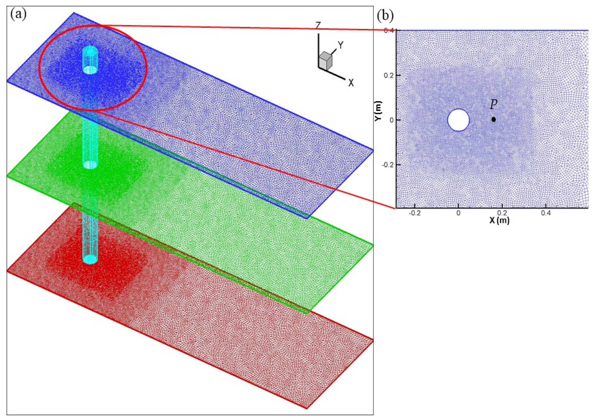
A three-layer hydrostatic model was used to simulate the von Karman vortex shedding. The length and width of the study domain were 2.4 m and 0.8 m, respectively. A circular obstacle with a radius of 0.05 m was located in the center of the mainstream—see Figure 1. The still water depth h = 0.1 m. Inflow was uniformly divided into three layers. The inflow entered the domain from the left boundary, and exited the domain from the right open boundary. The inflow speed increased linearly from bottom layer to top layer, i.e., U = 0.33 ms⁻¹, 0.67 ms⁻¹, and 1.00 ms⁻¹ in the bottom, middle, and top layer, respectively. Free slip boundary condition was employed for both top and bottom boundaries, and a non-slip boundary condition was enforced on the cylinder surface. The resulting Reynolds number was Re = 100, 200, and 300 in the bottom, middle, and top layer, respectively.

Figure 1 shows the computational meshes, a total of 24,582 nodes and 24,317 four-node quadrilateral elements. Nodal connection and mesh structure were the same for each layer. Finer meshes were used near the cylinder area because variation of flow and wave in that area was expected significantly. Δt = 0.025 s was used in the computations. Simulation started with a motionless fluid, i.e., the fluid was at rest initially. Flow developed and reached a periodic state after a period of about 200 s of transition.

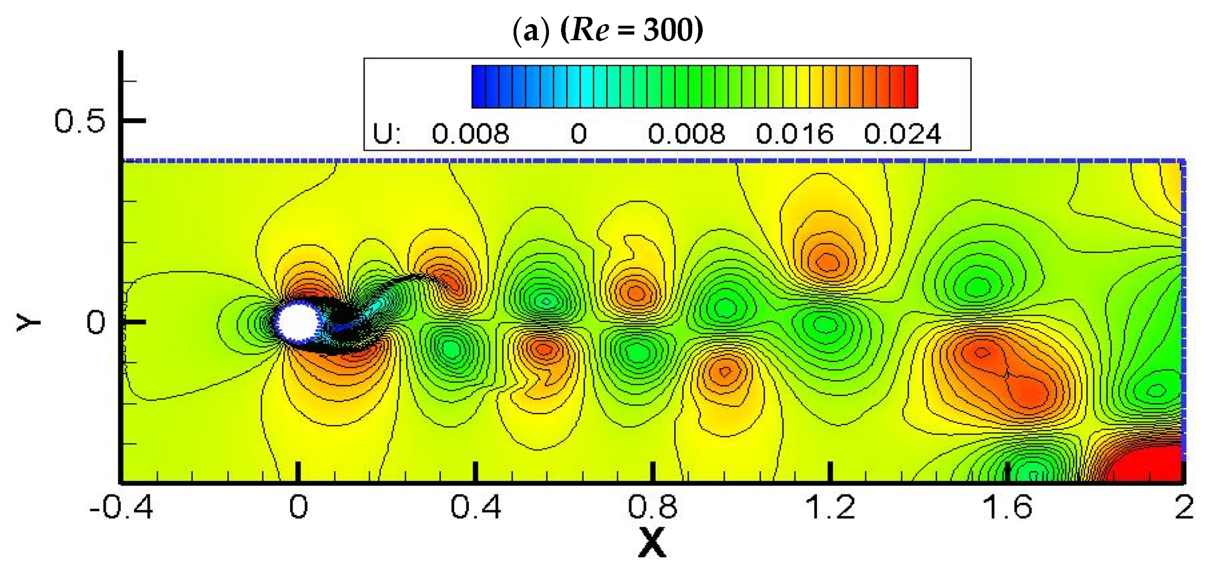
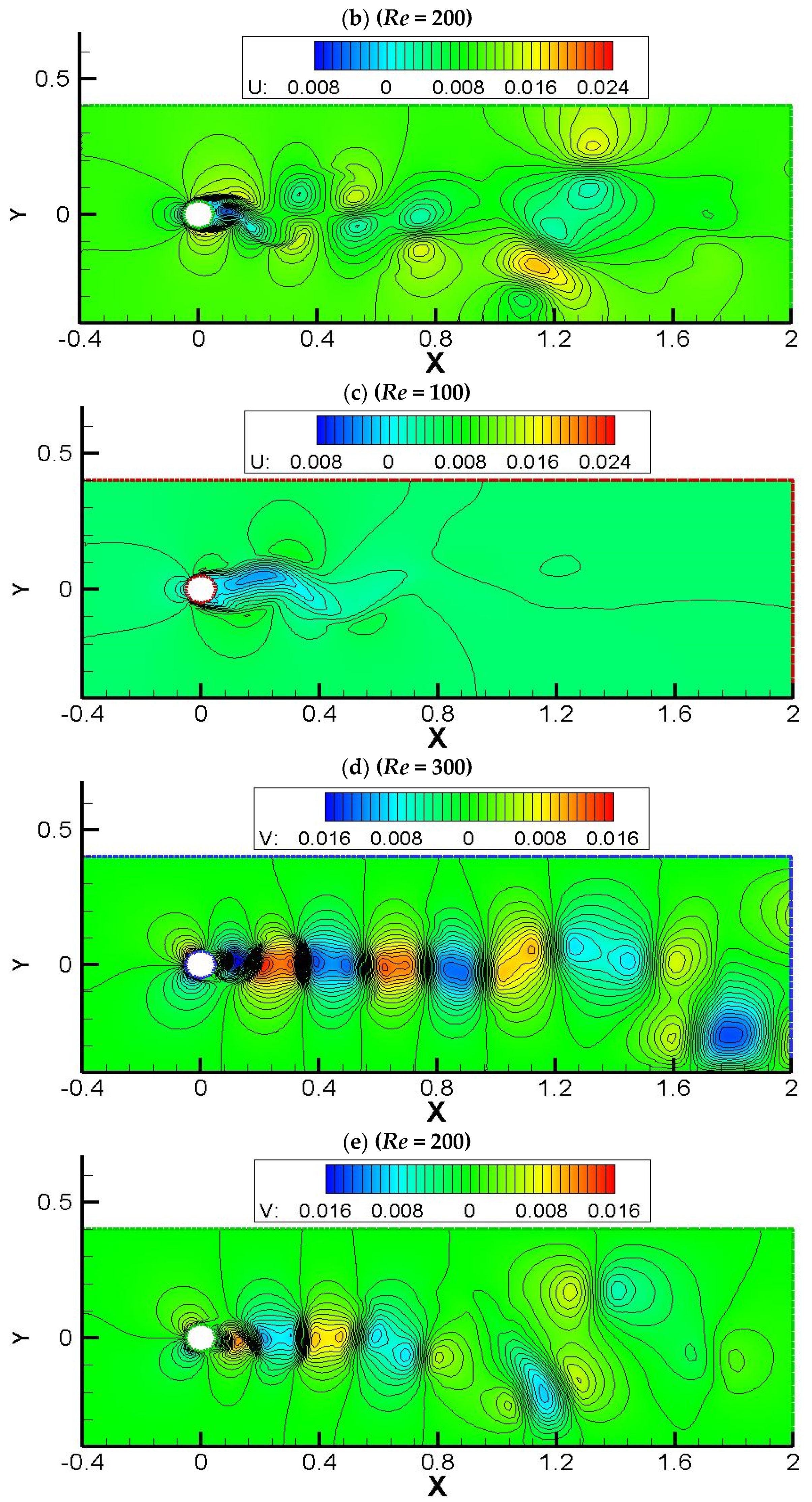
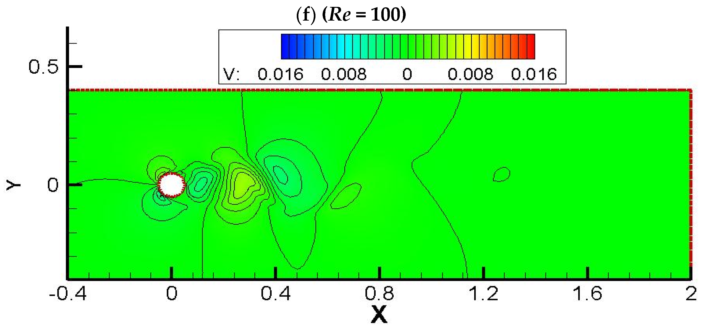
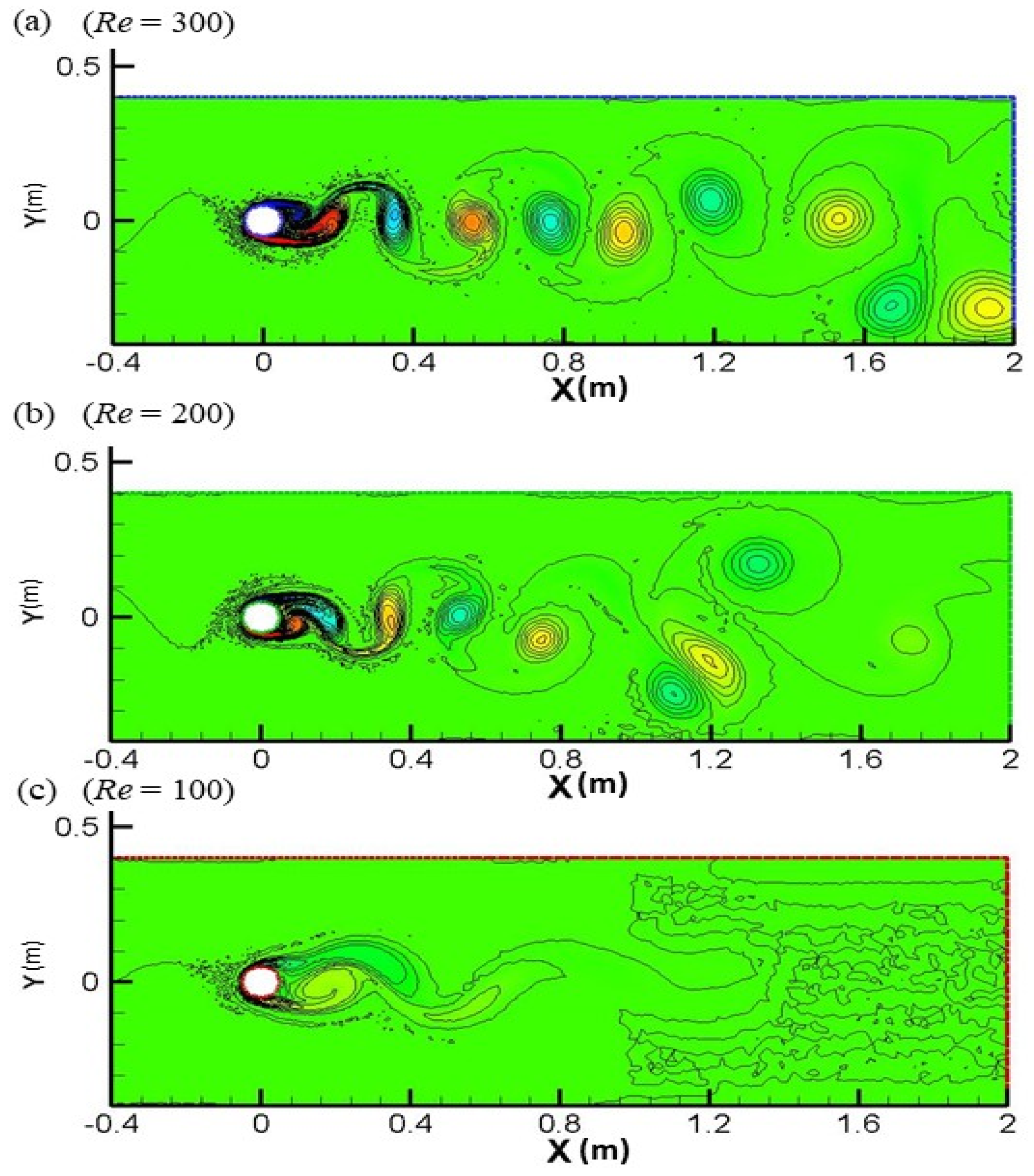
Figure 2 plots the U- and V-contours of each layer. The magnitude of flow of the top layer was larger than that of the middle and bottom layer. Periodic and well-organized alternating counter-rotating vortices were reproduced. The size of the vortex street of the top layer was longer and wider than those of the middle and bottom layer. The repeat (frequency) of U-contours was twice that of V-contours. This is one of the typical characteristics of a von Karman vortex street. Figure 3 depicts the contours of vorticity of each layer. The strength of vorticity was large in the top layer, and it decreased downstream. Well-organized alternating counter-rotating vortices were clearly observed.

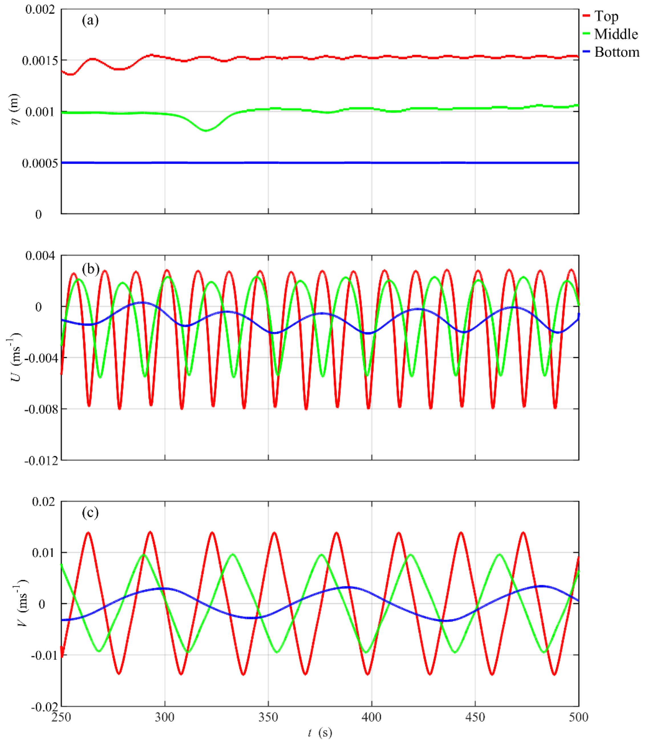
Figure 4 depicts the time history of η, U and V of the monitor point P (location of the monitor point P is shown in Figure 1b) of the top, middle, and bottom layers, respectively. The temporal variation of η was very small for this problem setting, and the temporal variation of U and V of each layer was quite different. The periods of U and V of the top, middle, and bottom layers were 15.6, 22.7, and 45.5 s, as well as 30, 43, and 92 s, respectively. The period of V is about twice of that of U. The corresponding averaged Strouhal number (St = D/UT) was 0.224, which agreed well with the value of 0.232, suggested by Williamson [2].

3.2. Green Island Vortex Shedding

There are two main islands in the southeast Taiwan water. The larger one is Orchid Island, which is located at 22°03′ N 121°32′ E, about 90 km off the southeast coast of Taiwan. It covers an area about 45 km², with a diameter of about 13.5 km. The smaller one is Green Island, which is located at 22°40′ N 121°28′ E, about 45 km off the southeast coast of Taiwan. It covers an area about 15 km², with a diameter about 5.5 km.

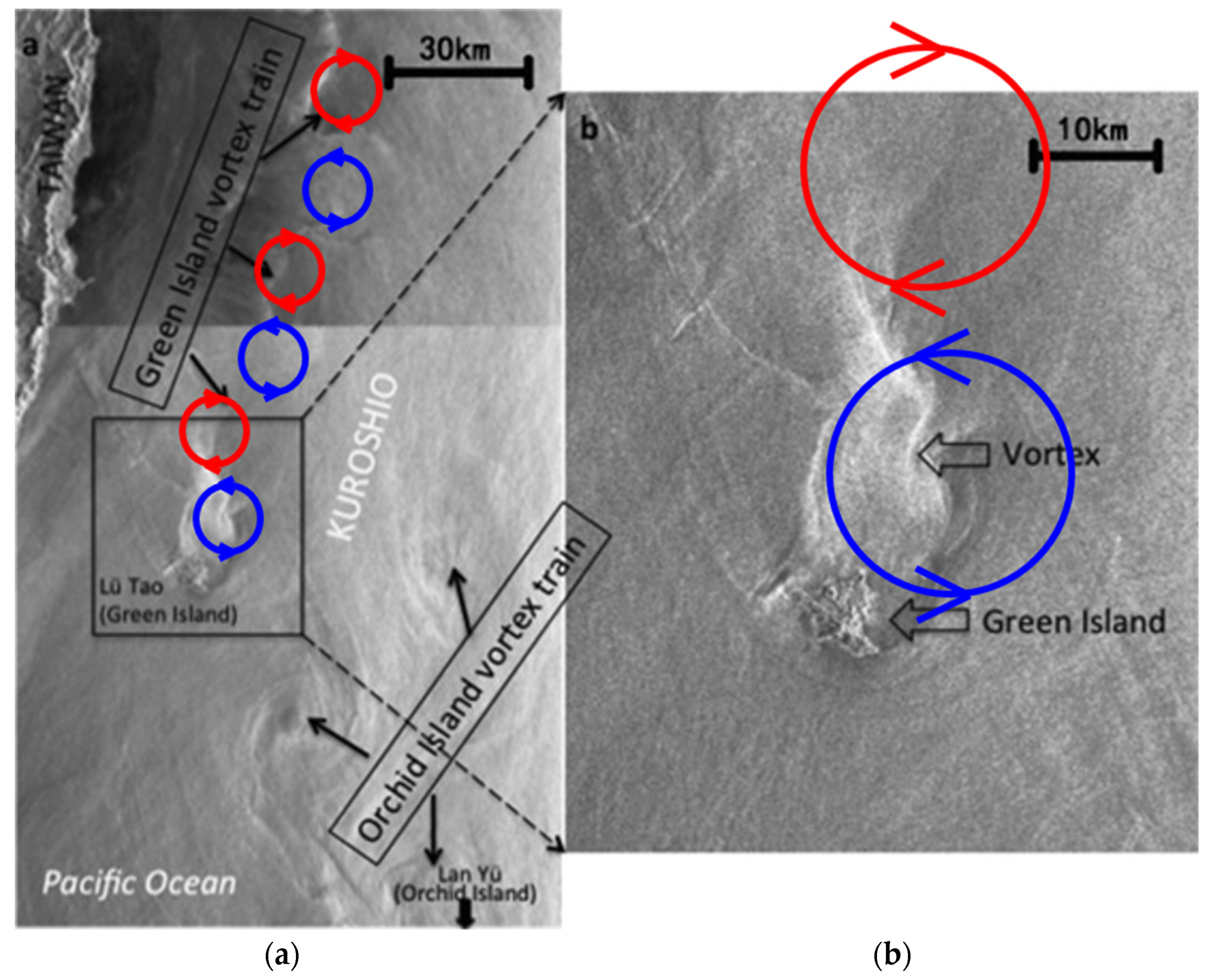
Primary package components of ADCP-CTD include a conductivity–temperature–depth (CTD) instrument and an acoustic Doppler current profiler (ADCP), allowing for the simultaneous measurement of density, water-mass tracers, and absolute velocity. Shipboard ADCP-CTD profiling was conducted to investigate the surface patterns, vertical structures, the evolution of the Green Island vortices [22,23]. The ERS-1 SAR images and Moderate-resolution Imaging Spectroradiometer (MODIS) satellite images [24,25,26,27], and numerical modelling [28,29,30,31,32] have also been used to study Kuroshio-induced island vortex of Orchid Island and Green Island. Figure 5a shows a composite ERS-1 SAR image of the Kuroshio-induced vortex of Orchid Island and Green Island, taken in one-week intervals, sequentially, at 17:01 UT September 25 (lower, with lighter colour background) and 19:02 UT 2 October 1996 (top, with darker colour background). The horizontal scale of the Orchid Island vortex street was about 50–70 km (about 3–5 times size of the island) in the streamwise direction, and 20–35 km (1.5–2.5 times size of the island) in the spanwise direction. While the horizontal scale of Green Island vortex street was about 50–60 km (8–10 times size of the island) in the streamwise direction, and 10–20 km (2–3 times size of the island) in the spanwise direction.

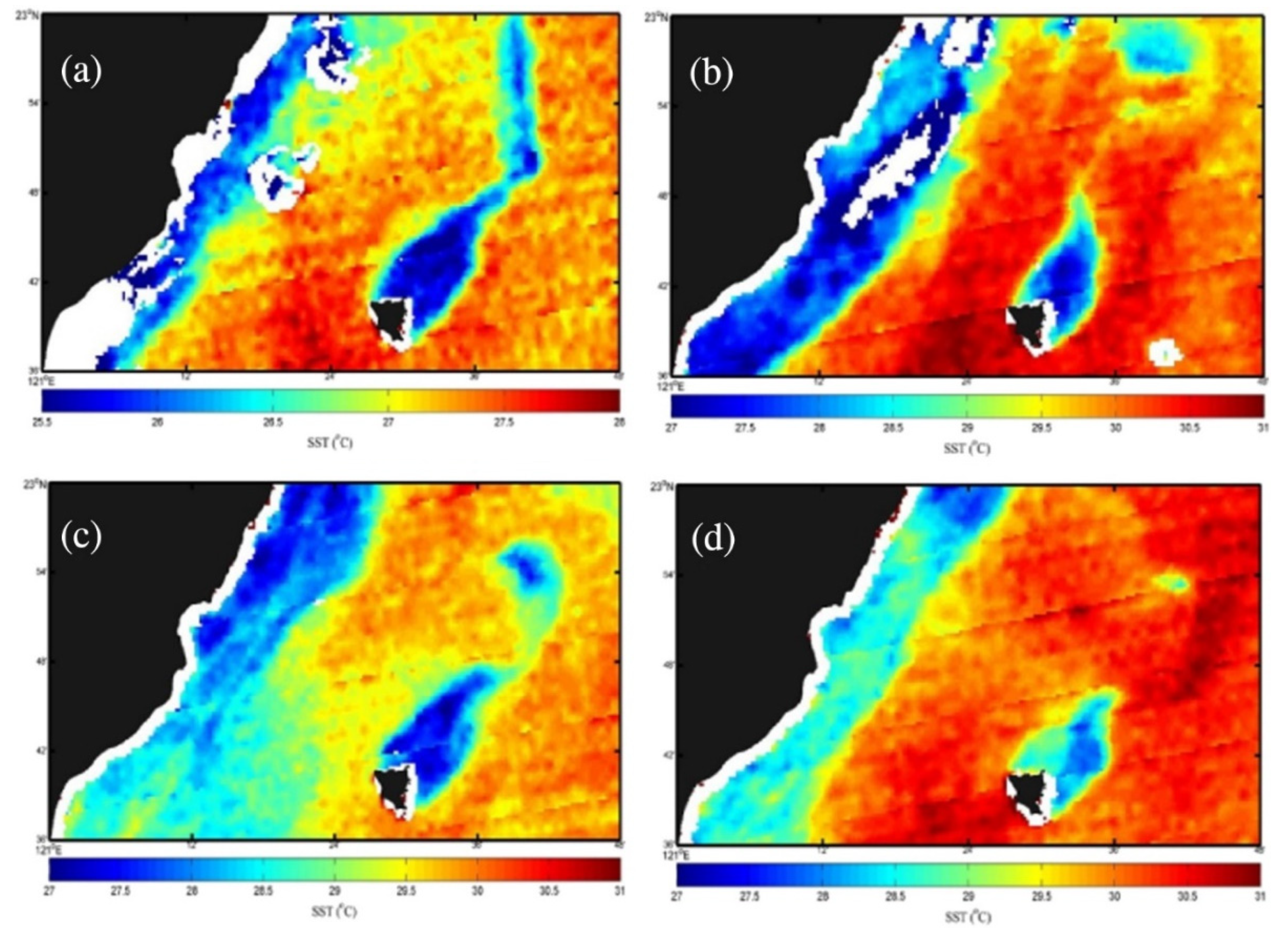
Current-induced vortices are associated with upwelling or vertical mixing, which causes cooler water to rise [22,63]. Figure 6 illustrates the Kuroshio-induced Green Island vortex using the sea surface temperature (SST) of MODIS Aqua images [25]. A recirculation zone covering area about 2–3 times the size of the island behind the island is clearly shown, following a meandering vortex street extending to about 6–8 times the size of the island downstream. Chang et al. [22] measured the SST of the recirculating water using shipboard ADCP-CDT, and found that the SST of the recirculating water was 1–2 °C colder than the SST of the surrounding waters.

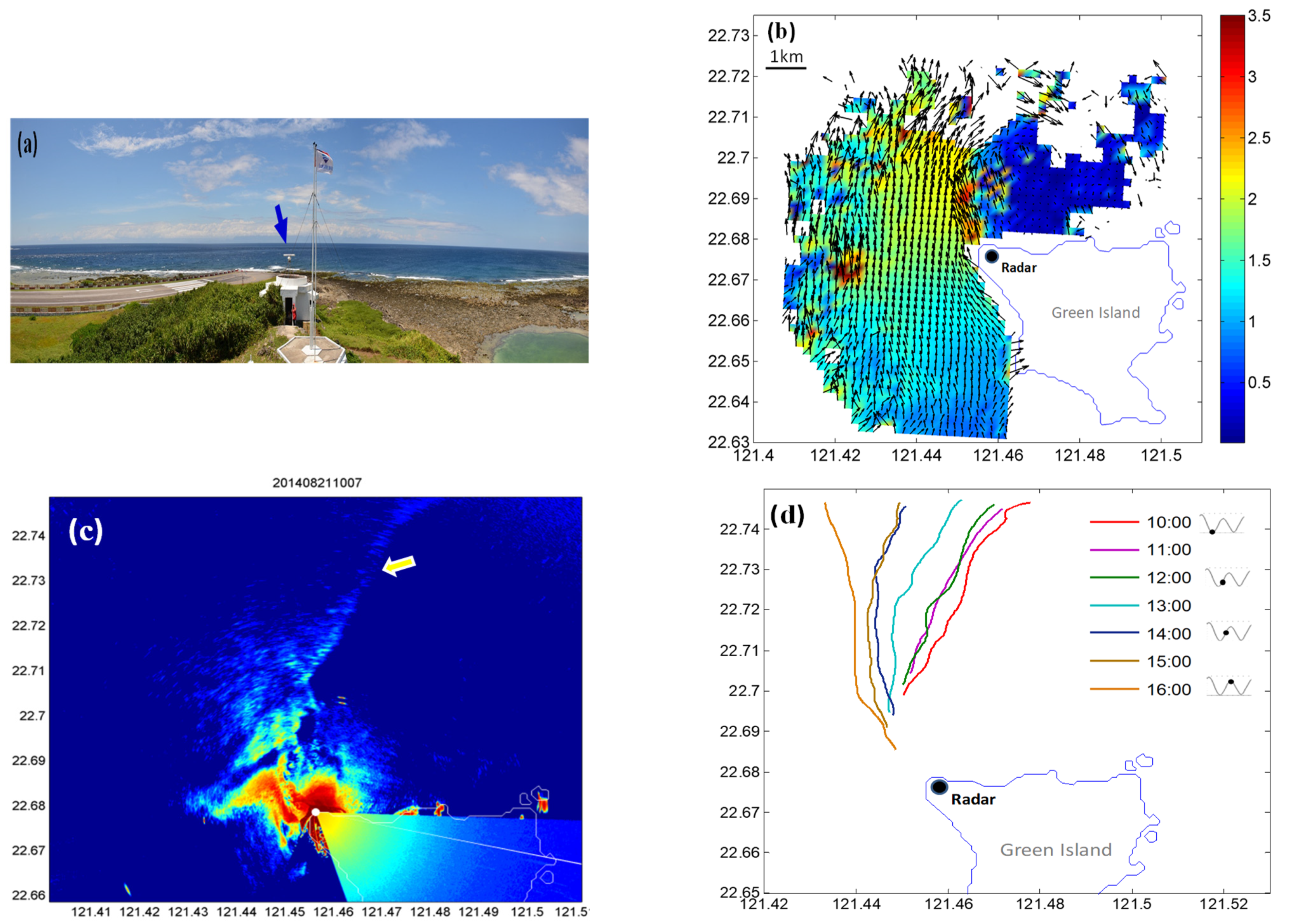
An observation study of Green Island wakes has been conducted using a land-based X-band marine radar system to measure the surface currents near the northwest of the island from 18 to 25 August 2014 [64] (see Figure 7a). The observation area covers an area with a diameter of about 10 km. The surface current can be derived from the radar backscatter by applying the wave dispersion relationship as the filter [65]. When Kuroshio passed the island (the surface speed is 1–1.5 ms⁻¹), a swirling recirculation was formed behind the island. The size of the recirculated water was about 1–1.5 times the size of the island, as shown in Figure 7b. This value is smaller than the value of 2–3 times the size of the island that was reported in [25] by analyzed satellite images. The speed of the Kuroshio current on the left-hand side downwind of the island was large, reaching 2–3 ms⁻¹. However, the surface current speed in the recirculation zone was less than 0.6 ms⁻¹ because of the blockage and shield of the island. The edge of the vortex street was identified by edge detection approach of the time-averaged radar images (see Figure 7c). The swing edge of the vortex shedding was time varying (see Figure 7d). The period of the swinging vortex shedding was estimated to be about 13 h.

3.3. Numerical Study

A depth-averaged one-layer hydrostatic shallow-water model was developed and applied to simulate the Green Island wakes in a previous study [28,29,30]. A high-resolution model is required to simulate the small-scale Green Island vortices (with sizes about 15–25 km in the streamwise direction, and 10–15 km in the spanwise direction) which are much smaller than the mesoscale ocean eddies with sizes of 100–500 km. In this study, a high-resolution (100–1200 m) three-layer shallow-water model was used to study the Green Island vortices and their interactions with the Orchid Island vortices.

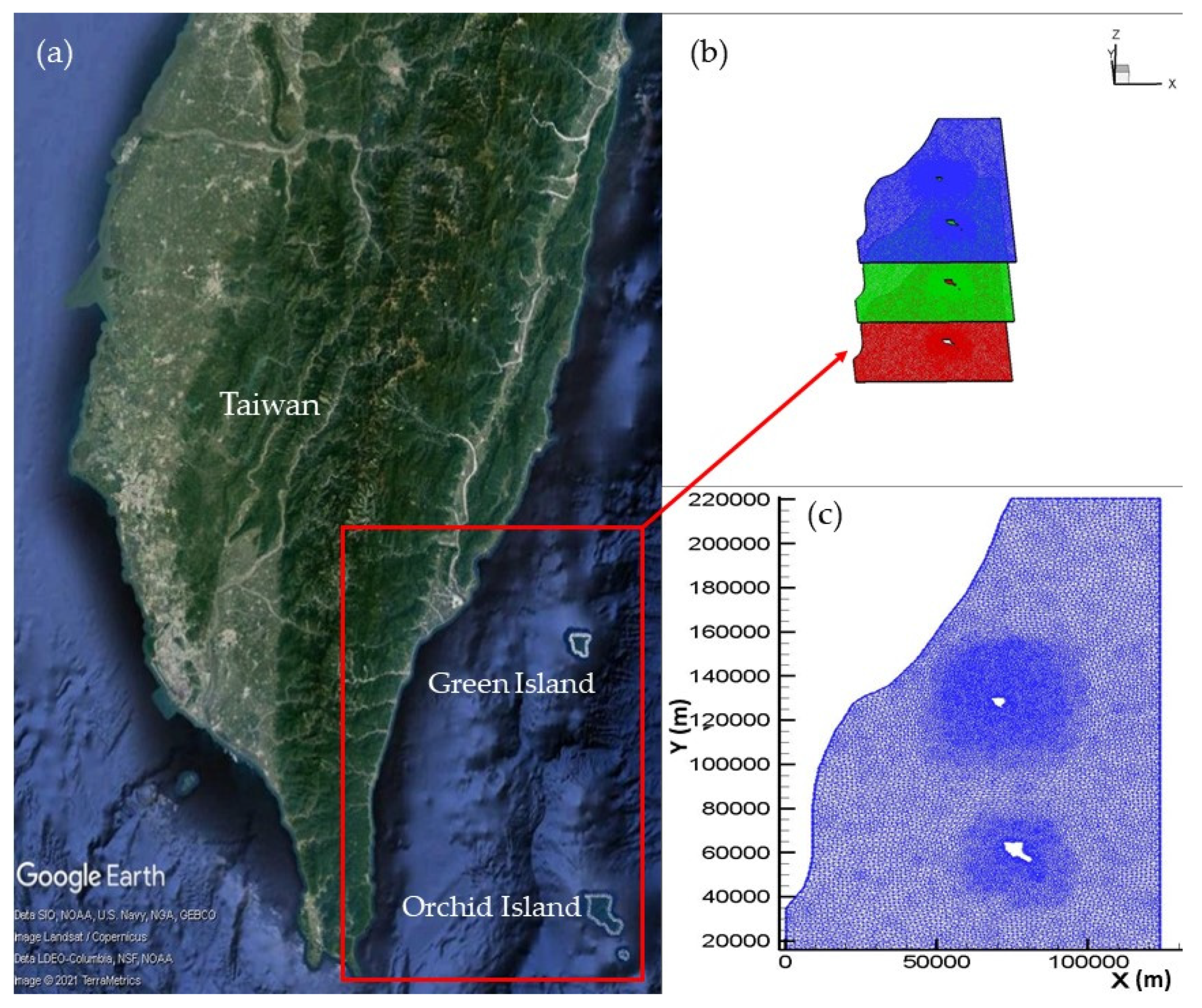
Figure 8a depicts the study area, with a length of about 220 km and a width of about 120 km. The Kuroshio current originates from the North Equatorial Current. It flows northward, parallel to the eastern coast of Taiwan, and passes Orchid Island and Green Island. The width of Kuroshio is about 100–150 km. According to the field measurements [22,25] and satellite image analysis [30], the speed of the Kuroshio current is about 1.0 ms⁻¹ in the top layer (0 m to −200 m), 0.5 ms⁻¹ in the middle layer (−200 m to −400 m), and 0.3 ms⁻¹ in the bottom layer (−400 m to −700 m). The influence range of the Kuroshio current is up to −800 m: water below −800 m is essentially motionless.

The top layer ranges from 0 m to −250 m, the middle layer from −250 m to −500 m, and the bottom layer −500 m from to −750 m. The speed of Kuroshio current is 1.00 ms⁻¹ in the top layer, 0.67 ms⁻¹ in the middle layer, and 0.33 ms⁻¹ in the bottom layer. This information was used in the simulations. Kuroshio enters the study area from the south boundary and exits the north boundary freely. On the west boundary, to the southeast of Taiwan, slip boundary condition was employed, and on the east boundary no normal flux condition was employed. A non-slip boundary condition was specified for both Orchid Island and Green Island.

Figure 8b shows the computational meshes, a total of 53,170 nodes and 13,166 nine-node quadrilateral elements. Fine meshes are used near the area of Orchid Island and Green Island, since significant variations of flow and waves are expected in these areas (see Figure 8c). Δt = 15 s was used in the modelling. The simulation started with motionless fluid, i.e., fluid was at rest initially. After a period of transition, about 30 h, recirculation and island-induced vortices developed, and flow reached a periodic state.

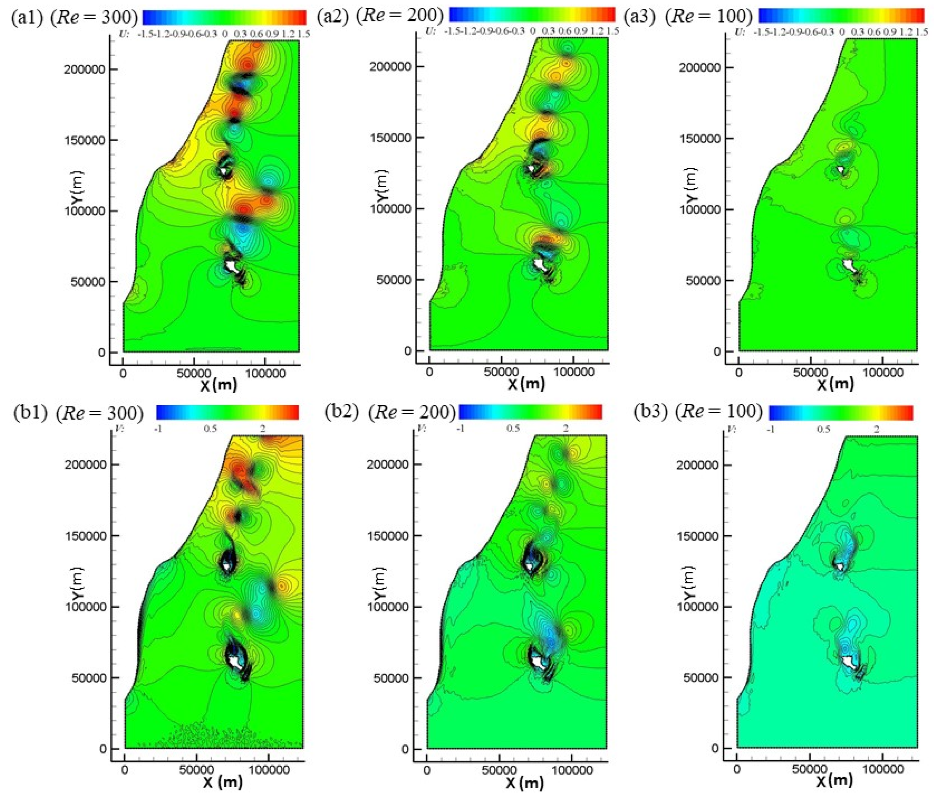
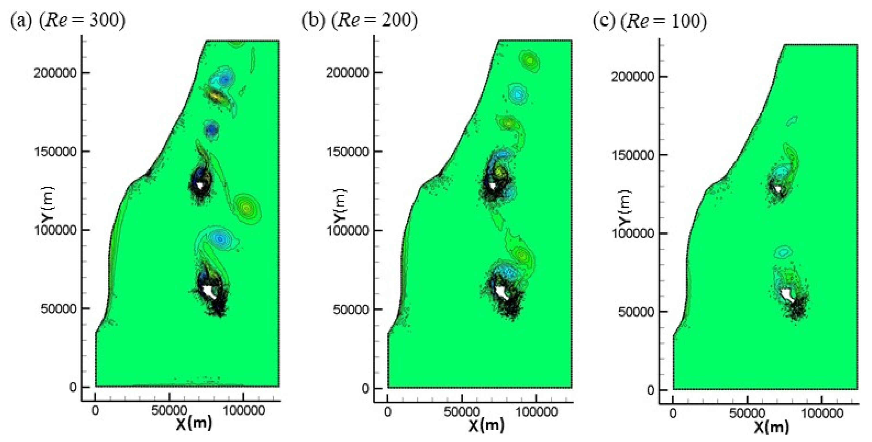
Figure 9 depicts the U- and V-contours of the top, middle, and bottom layers, respectively. The magnitude of current of the bottom layer was smaller than that of the middle and top layers. A recirculation of the top layer, with a size about 1–2 time of the island, was formed behind the island. It followed three pairs of alternating counter-rotating vortices that extended about 50–60 km (8–10 times the size of the island); two pairs of alternating counter-rotating vortices that extended about 30–50 km (5–8 times the size of the island); and one alternating counter-rotating vortices that extended about 15–30 km (2–5 times the size of the island) downstream of the top, middle, and bottom layer, respectively. Green Island is located about 60 km downstream of the Orchid Island vortex street. Green Island vortices of the top layer were obviously affected by the upstream Orchid Island vortices, also revealed in Figure 10 and Figure 11. However, the Green Island vortices of the middle and bottom layers seemed less affected by the Orchid Island vortices of the middle and bottom layers, respectively.

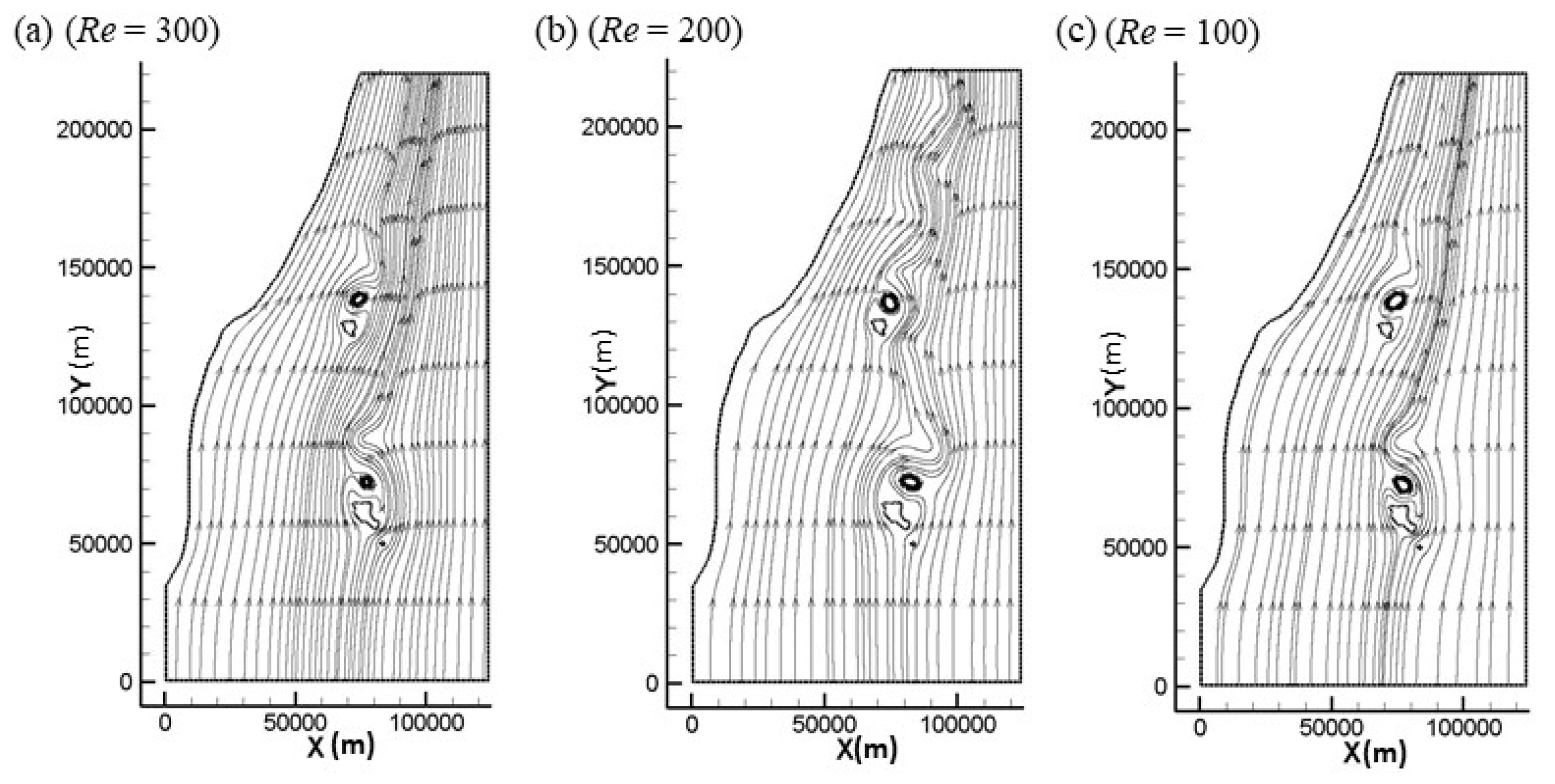
Figure 10 and Figure 11 show the contours, streamlines and vorticity of the top, middle, and bottom layers, respectively. Vortices of the top layer were larger than that of the middle and bottom layers. The vortex street of the top layer was longer and wider than that of the middle and bottom layers. The periods of top layer vortex shedding for Orchid Island and Green Island were found to be 32.8 and 14.5 h, respectively. The period of Orchid Island vortex shedding was larger than that of Green Island, due to its larger size, and therefore the larger Reynolds number of Orchid Island. The value of 14.5 h for the period of the top layer of Green Island vortex shedding agreed reasonably with the value of 13 h by the land-based X-band radar measurement [64].

3.4. Discussion

The least-square finite element method exhibits many theoretical, programming and computational advantages. For example, because of the use of a single approximating space for all variables, and the choice of approximating spaces not subjected to the Ladyzhenskaya–Babuska–Brezzi (LBB) condition, mixed formulation, collocation grid arrangement, and convection schemes are unnecessary [60,62]. Moreover, the resulting system of equations is symmetric and positive–definite, and therefore can be effectively solved by the preconditioned conjugate gradient method [66]. Advantages and details of the least-squares finite element method can be found in [60,62].

Deep water or stratified flows may experience large vertical flow variations. Strong dispersive or non-linear waves propagating shoreward may undergo significant wave deformation caused by variations in water depth or bottom friction. These phenomena may not well be presented in the nonlinear hydrostatic shallow-water models. Thus, it is often indispensable to consider non-hydrostatic effects in modelling free surface flows with large vertical variations, especially for both deep-water flows and short waves with high non-linearity. A number of non-hydrostatic coastal ocean models have been developed [44,45,46,47,48,49,50,51,52,53,54]. A depth-averaged (one-layer) non-hydrostatic shallow-water model was developed and applied to model the propagation of a solitary wave and the interactions of the propagating solitary wave with the submerged structure in a previous study [67]. Computed results showed the promising potential of the model.

Flows and waves of the surface and subsurface are more interesting and important, as well as easier to measure, in general. However, vertical variations and structures of flows and waves could be of importance in many situations, such as underwater coastal structures, sedimentations, anchored platforms, etc. The development and application of a multi-layer non-hydrostatic free-surface model for coastal environments is a focus of future study. The multi-layer non-hydrostatic modelling approach solves 2D layer-integrated equations, instead of solving 3D equations [56,57]; therefore, it is considered computationally efficient. Furthermore, only a relatively small number of vertical layers are required to enable the accurate simulation of vertically varying flows, as well as dispersive and nonlinear waves, in general.

4. Conclusions

In this paper, we present the formulation, development, and application of a multi-layer depth-integrated nonlinear hydrostatic shallow-water model for free-surface flows, with vertical variations using the θ time integration method and the least-square finite element method. The model was applied to simulate a von Karman vortex street and a Kuroshio-induced Green Island vortex.

Computed results of Green Island vortices showed that the vortices of the top layer were stronger than those of the middle and bottom layers. A recirculation was formed behind the island, with a size about 1.5 times the size of the island (agreeing with the value of 1.5 times the size of the island by the X-band radar measurement [64], and the modelling results of [28,29,30,34], but smaller than value of 2–3 times the size of the island by the analysis of satellite images [25]). The speed of the recirculation (~0.5 ms⁻¹) was small, due to the blockage and shield of the island (agreeing with the ADCP measurement [22] and the X-band radar measurement [64]). The streamwise and spanwise size of the Green Island vortex street of the top layer were 50–60 km and 10–15 km (agreeing with the value of 50–60 km and 10–20 km by the analysis of satellite imageries [24,25], and larger than value of 40–50 km and 10–20 km by the one-layer modelling results of [28,29,30,34]). The period of Green Island vortex shedding was 14.5 h (larger than the value of 13 h by the X-band radar measurement [64]). It was revealed that Green Island vortices were affected by the upstream Orchid Island vortices. This result was supported by the field measurement of [22].

An immediate next step is to extend the present model for multi-layer non-hydrostatic nonlinear shallow-water equations into future study, so that large vertically varying flows and highly dispersive waves can be better approximated. With the recent theory development of computational fluid dynamics, and the advancement of computer hardware, the simulation of large scale and complicated realistic fluid flows and waves is feasible.

References

- Tritton, D.J. Experiments on the flow past a circular cylinder at low Reynolds numbers. J. Fluid Mech. 1959, 6, 547–567. [Google Scholar] [CrossRef]
- Williamson, C.H.K. Oblique and parallel modes of vortex shedding in the wake of a circular cylinder at low Reynolds numbers. J. Fluid Mech. 1989, 206, 579. [Google Scholar] [CrossRef] [Green Version]
- Williamson, C.H. Vortex dynamics in the cylinder wake. Annu. Rev. Fluid Mech. 1996, 28, 477–539. [Google Scholar] [CrossRef]
- Zdravkovich, M.M. Flow around Circular Cylinders; Oxford University Press: Oxford, UK, 1997; ISBN 0198563965. [Google Scholar]
- Peter, A. Vortices and tall buildings: A recipe for resonance. Phys. Today 2010, 63, 9. [Google Scholar]
- Hubert, L.; Krueger, A. Satellite pictures of mesoscale eddies. Mon. Weather Rev. 1962, 90, 457–463. [Google Scholar] [CrossRef]
- Thomson, R.E.; Gower, J.F.; Bowker, N.W. Vortex streets in the wake of the Aleutian Islands. Mon. Weather Rev. 1977, 105, 873–884. [Google Scholar] [CrossRef] [Green Version]
- Li, X.F.; Clemente-Colon, P.; Pichel, W.G.; Vachon, P.W. Atmospheric vortex streets on a RADARSAT SAR image. Geophys. Res. Lett. 2000, 27, 1655–1658. [Google Scholar] [CrossRef]
- Young, G.S.; Zawislak, J. An observational study of vortex spacing in island wake vortex streets. Mon. Weather Rev. 2006, 134, 2285–2294. [Google Scholar] [CrossRef]
- Topouzelis, K.; Kitsiou, D. Detection and classification of mesoscale atmospheric phenomena above sea in SAR imagery. Remote Sens. Environ. 2015, 160, 263–272. [Google Scholar] [CrossRef]
- Barkley, R.A. Johnston atolls wake. J. Mar. Res. 1972, 30, 201–216. [Google Scholar]
- Wolanski, E.; Imberger, J.; Heron, M. Island wakes in shallow coastal waters. J. Geophys. Res. Ocean. 1984, 89, 10553–10569. [Google Scholar] [CrossRef]
- Heywood, K.J.; Stevens, D.P.; Bigg, G.R. Eddy formation behind the tropical island of Aldabra. Deep Sea Res. Part I 1996, 43, 555–578. [Google Scholar] [CrossRef] [Green Version]
- Dong, C.M.; McWilliams, J.C.; Shchepetkin, A.F. Island wakes in deep water. J. Phys. Oceanogr. 2007, 37, 962–981. [Google Scholar] [CrossRef]
- Zheng, Q.; Lin, H.; Meng, J.M.; Hu, X.M.; Song, Y.T.; Zhang, Y.Z.; Li, C.Y. Sub-mesoscale ocean vortex trains in the Luzon Strait. J. Geophys. Res. Ocean. 2008, 113, C04032. [Google Scholar] [CrossRef] [Green Version]
- Chelton, D.B.; Schlax, M.G.; Samelson, R.M. Global observations of nonlinear mesoscale eddies. Prog. Oceanogr. 2011, 91, 167–216. [Google Scholar] [CrossRef]
- Zheng, Q.; Holt, B.; Li, X.F.; Liu, X.N.; Zhao, Q.; Yuan, Y.L.; Yang, X.F. Deep-water seamount wakes on SEASAT SAR image in the Gulf stream region. Geophys. Res. Lett. 2012, 39, L16604. [Google Scholar] [CrossRef]
- Robinson, A.R.; McGillicuddy, D.J.; Calman, J.; Ducklow, H.W.; Fasham, M.J.R.; Hoge, F.E.; Leslie, W.G.; McCarthy, J.J.; Podewski, S.; Porter, D.L.; et al. Mesoscale and upper ocean variabilities during the 1989 JGOFS bloom study. Deep Sea Res. Part II Top. Stud. Oceanogr. 1993, 40, 9–35. [Google Scholar] [CrossRef]
- Faghmous, J.H.; Frenger, I.; Yao, Y.; Warmka, R.; Lindell, A.; Kumar, V. A daily global mesoscale ocean eddy dataset from satellite altimetry. Sci. Data 2015, 2, 150028. [Google Scholar] [CrossRef] [Green Version]
- Sorgente, R.; Olita1, A.; Oddo, P.; Fazioli1, L.; Ribotti, A. Numerical simulation and decomposition of kinetic energy in the Central Mediterranean: Insight on mesoscale circulation and energy conversion. Ocean Sci. 2011, 7, 503–519. [Google Scholar] [CrossRef] [Green Version]
- Dietze, H.; Matear, R.; Moore, T. Nutrient supply to anticyclonic meso-scale eddies off western Australia estimated with artificial tracers released in a circulation model. Deep-Sea Res. Pt. I 2009, 56, 1440–1448. [Google Scholar] [CrossRef]
- Chang, M.H.; Tang, T.Y.; Ho, C.R.; Chao, S.Y. Kuroshio-induced wake in the lee of Green Island of Taiwan. J. Geophys. Res. Ocean. Atmos. 2013, 118, 1508–1519. [Google Scholar] [CrossRef]
- Chang, M.H.; Jan, S.; Mensah, V.; Andres, M.; Rainville, L.; Yang, Y.J. Zonal migration and transport variations of the kuroshio east of Taiwan induced by eddy impingements. Deep Sea Res. Part I Oceanogr. Res. Pap. 2018, 131, 1–15. [Google Scholar] [CrossRef]
- Zheng, Z.W.; Zheng, Q. Variability of island-induced ocean vortex trains, in the Kuroshio region southeast of Taiwan Island. Cont. Shelf Res. 2014, 81, 1–6. [Google Scholar] [CrossRef]
- Hsu, P.C.; Chang, M.H.; Lin, C.C.; Huang, S.J.; Ho, C.R. Investigation of the island-induced ocean vortex train of the Kuroshio current using satellite imagery. Rem. Sens. Environ. 2017, 193, 54–64. [Google Scholar] [CrossRef]
- Hsu, P.C.; Cheng, K.H.; Jan, S.; Lee, H.J.; Ho, C.R. Vertical structure and surface patterns of green island wakes induced by the Kuroshio. Deep Sea Res. Part I Oceanogr. Res. Pap. 2019, 143, 1–16. [Google Scholar] [CrossRef]
- Hsu, P.C.; Ho, C.Y.; Lee, H.J.; Lu, C.Y.; Ho, C.R. Temporal variation and spatial structure of the Kuroshio-induced submesoscale island vortices observed from GCOM-C and Himawari-8 data. Rem. Sens. 2020, 12, 883. [Google Scholar] [CrossRef] [Green Version]
- Liang, S.J.; Lin, C.Y.; Hsu, T.W.; Ho, C.R.; Chang, M.H. Numerical study of vortex characteristics near Green Island, Taiwan. J. Coast. Res. 2013, 29, 1436–1444. [Google Scholar]
- Huang, S.J.; Ho, C.R.; Lin, S.L.; Liang, S.J. Spatial-temporal scales of Green Island wake due to passing of the Kuroshio current. Int. J. Rem. Sens. 2014, 35, 4484–4495. [Google Scholar] [CrossRef]
- Hsu, T.W.; Doong, D.J.; Hsieh, K.J.; Liang, S.J. Numerical study of Monsoon effecton Green Island Wake. J. Coast. Res. 2015, 31, 1141–1150. [Google Scholar] [CrossRef]
- Hou, T.H.; Chang, J.Y.; Tsai, C.C.; Hsu, T.W. 3D Numerical Simulation of Kuroshio-induced wake near Green Island, Taiwan. J. Mar. Sci. Tech. TAIW 2020, 29, 7. [Google Scholar] [CrossRef]
- Hou, T.H.; Chang, J.Y.; Tsai, C.C.; Hsu, T.W. Three-Dimensional Simulations of Wind Effects on Green Island Wake. Water 2020, 12, 3039. [Google Scholar] [CrossRef]
- Chen, F. The Kuroshio Power Plant; Springer: Cham, Switzerland, 2013. [Google Scholar]
- Hsu, T.W.; Liau, J.M.; Liang, S.J.; Tzang, S.Y.; Doong, D.J. Assessment of Kuroshio current power test site of Green Island, Taiwan. Renew. Energy 2015, 81, 853–863. [Google Scholar] [CrossRef]
- Phillips, O.M. The Dynamics of the Upper Ocean; Cambridge University Press: Cambridge, UK, 1977. [Google Scholar]
- Kinnmark, I. The Shallow-Water Wave Equations: Formulation, Analysis and Application; Springer: Berlin, Germany, 1986. [Google Scholar]
- Mei, C.C. The Applied Dynamics of Ocean Surface Waves; World Scientific: Singapore, 1989. [Google Scholar]
- Tan, W.Y. Shallow Water Hydrodynamics: Mathematical Theory and Numerical Solution fora Two-Dimensional System of Shallow-Water Equations; Elsevier: Singapore, 1992. [Google Scholar]
- Martin, J.L.; McCutcheon, S.C. Hydrodynamics and Transport for Water Quality Modeling; CRC Press: Boca Raton, FL, USA, 1998. [Google Scholar]
- Vreugdenhil, C.B. Numerical Methods for Shallow-Water Flow; Springer Science & BusinessMedia: Singapore, 2013. [Google Scholar]
- Peregrine, D.H. Long waves on a beach. J. Fluid Mech. 1967, 27, 815–827. [Google Scholar] [CrossRef]
- Nwogu, O. Alternative form of Boussinesq equations for nearshore wave propagation. J. Waterw. Port. Coast. Ocean. Eng. 1993, 119, 618–638. [Google Scholar] [CrossRef] [Green Version]
- Madsen, P.A.; Murray, R.; Sorensen, O.R. A new form of the Boussinesq equations with improved linear dispersion characteristics. Coast. Eng. 1991, 15, 371–388. [Google Scholar] [CrossRef]
- Casulli, V. Semi-implicit finite difference methods for two-dimensional shallow water equations. J. Comput. Phys. 1990, 86, 56–74. [Google Scholar] [CrossRef]
- Casulli, V.; Stalelling, G.S. Numerical simulation of 3D quasi-hydrostatic, free surface flows. J. Hydraul. Eng. 1998, 124, 678–686. [Google Scholar] [CrossRef]
- Casulli, V. A semi-implicit finite difference method for non-hydrostatic, free surface flows. Int. J. Numer. Methods Fluids 1999, 30, 425–440. [Google Scholar] [CrossRef]
- Namin, M.M.; Lin, B.; Falconer, R.A. An implicit numerical algorithm for solving non-hydrostatic free-surface flow problems. Int. J. Numer. Methods Fluids 2001, 35, 341–356. [Google Scholar] [CrossRef]
- Casulli, V.; Zanolli, P. Semi-implicit numerical modeling of nonhydrostatic free surface flows for environmental problems. Math. Comput. Model. 2002, 36, 1131–1149. [Google Scholar] [CrossRef]
- Lin, P.; Li, C.W. A σ-coordinate three-dimensional numerical model for surface wave propagation. Int. J. Numer. Meth. Fluids 2002, 38, 1045–1068. [Google Scholar] [CrossRef]
- Zijlema, M.; Stelling, G.S. Further experiences with computing non-hydrostatic free-surface flows involving water waves. Int. J. Numer. Methods Fluids 2005, 48, 169–197. [Google Scholar] [CrossRef]
- Waters, R.A. A semi-implicit finite element model for non-hydrostatic (dispersive) surface waves. Int. J. Numer. Methods Fluids 2005, 49, 721–737. [Google Scholar] [CrossRef]
- Fringer, O.B.; Gerritsen, M.; Street, R.L. An unstructured-grid, finite-volume, nonhydrostatic, parallel coastal ocean simulator. Ocean Model. 2006, 14, 139–173. [Google Scholar] [CrossRef]
- Yamazaki, Y.; Kowalik, Z.; Cheung, K.F. Depth-averaged non-hydrostatic model for wave breaking and run-up. Int. J. Numer. Methods Fluids 2009, 61, 473–497. [Google Scholar] [CrossRef]
- Wei, Z.P.; Jia, Y.F. Simulation of nearshore wave processes by a depth-integrated non-hydrostatic finite element model. Coast. Eng. 2014, 83, 93–107. [Google Scholar] [CrossRef]
- Lynett, P.; Liu, P.L.F. A two-layer approach to wave modeling. Proc. R. Soc. Lond. Ser. A 2004, 460, 2637–2669. [Google Scholar] [CrossRef]
- Pan, W.; Kramer, S.C.; Piggott, M.D. Multi-layer non-hydrostatic free surface modelling using the discontinuous Galerkin method. Ocean Model. 2019, 134, 68–83. [Google Scholar] [CrossRef]
- Pan, W.; Kramer, S.C.; Matthew, D.; Piggott, M.D. A σ-coordinate non-hydrostatic discontinuous finite element coastal ocean Model. Ocean Model. 2021, 157, 101732. [Google Scholar] [CrossRef]
- Liang, S.J.; Tang, J.H.; Wu, M.S. Solution of shallow-water equations using least-squares finite-element method. Acta Mech. Sin. 2008, 24, 523–532. [Google Scholar] [CrossRef]
- Liang, S.J.; Hsu, T.W. Least-Squares finite-element method for shallow-water equations with source terms. Acta Mech. Sin. 2009, 25, 597–610. [Google Scholar] [CrossRef]
- Gunzburger, M. Finite Element Methods for Viscous Incompressible Flows: A Guide to Theory, Practice and Algorithms; NASA STI/Recon Technical Report A; Academic Press: Cambridge, MA, USA, 1989; Volume 91, p. 30750. [Google Scholar]
- Laible, J.P.; Pinder, G.F. Solution of the shallow water equations by least squares collocation. Water Resour. Res. 1993, 29, 445–455. [Google Scholar] [CrossRef]
- Jiang, B.-N. The Least-Squares Finite Element Method—Theory and Applications in Computational Fluid Dynamics and Electromagnetics; Springer: Berlin, Germany, 1998. [Google Scholar]
- Caldeira, R.M.A.; Marchesiello, P.; Nezlin, N.P.; DiGiacomo, P.M.; McWilliams, J.C. Island wakes in the Southern California Bight. J. Geophys. Res. Ocean. Atmos. 2005, 110, C11012. [Google Scholar] [CrossRef]
- Doong, D.J.; Wu, L.C. Use of Microwave Radar Backscatter for Green Island Wake Observation and Analysis. In Ministry of Science and Technology (MOST) of Taiwan Project Report; Ministry of Science and Technology (MOST) of Taiwan: Taipei, Taiwan, 2016. (In Chinese) [Google Scholar]
- Borge, J.C.N.; Reichert, K.; Dittmer, J. Use of nautical radar as a wave monitoring instrument. Coast. Eng. 1999, 37, 331–342. [Google Scholar] [CrossRef]
- Saad, Y. Iterative Methods for Sparse Linear Systems; SIAM: Philadelphia, PA, USA, 2003. [Google Scholar]
- Liang, S.J.; Young, C.C.; Dai, C.; Wu, N.J.; Hsu, T.W. Simulation of ocean circulation of Dongsha water using non-hydrostatic shallow-water model. Water 2020, 12, 2832. [Google Scholar] [CrossRef]
Figure 1.
Study domain and computational meshes: (a) global view and (b) close-up local view around the cylinder. Point P is the monitor point where flow variables are recorded. (Unit measurement for x and y axis is m).
Figure 2.
Contours of U (a–c) and V (d–f) of the von Karman vortex street of the top, middle, and bottom layer, respectively (U–contours range from −0.008 to 0.35 ms−1 with an interval 0.001 ms−1; V–contours range from −0.016 to 0.015 ms−1 with an interval 0.001 ms−1).
Figure 3.
Contours of vorticity (each plot consisted of 30 contours): (a) ranges from −0.165 to 0.122 of the top layer; (b) ranges from −0.089 to 0.088 of the middle layer; and (c) ranges from −0.032 to 0.025 of the bottom layer, respectively.
Figure 4.
Time history of η, U and V of the monitor point P (see Figure 1b) of (a) top, (b) middle, and (c) bottom layers, respectively.
Figure 5.
(a) A composite ERS-1 SAR image of Kuroshio-induced ocean vortex of Orchid Island and Green Island taken at 17:01 UT 25 September (lower, with lighter colour background) and 19:02 UT 2 October 1996 (top, with darker colour background). (b) Zoomed-in Green Island vortex (source: modified from Figure 2 of Zheng and Zheng [24]).
Figure 6.
Kuroshio-induced Green Island vortex by MODIS Aqua images at (a) 05:10 UTC on 4 April 2015, (b) 05:05 UTC on 16 June 2015, (c) 05:15 UTC on 30 June 2015, and (d) 05:05 UTC on 2 July 2015. (Source: Figure 7 of Hsu, et al. [25]).
Figure 7.
(a) Photo of the X-band marine radar observation system located to the northwest of Green Island. (b) Surface current speed near Green Island at 18:00, 19 August 2014. (c) Edge of vortex shedding detected from time averaged radar images. (d) Time varying edge of vortex shedding on 21 August 2014.
Figure 8.
(a) Schematic illustration of the study area. (b) Computational meshes of top, middle and bottom layer. (c) Close-up view of fine meshes near Orchid Island and Green Island where variations of flow and waves are significant.
Figure 9.
Contours of (a) U (upper panel) and (b) V (lower panel) of Orchid Island vortex and Green Island vortex of the (1) top (left panels), (2) middle (central panels), and (3) bottom (right panels) layer. (U–contours range from −1.5 to 1.5 ms−1 with an interval 0.1 ms−1; V-contours range from −1.2 to 2.6 ms−1 with an interval 0.1 ms−1).
Figure 10.
Streamlines of Orchid Island vortex and Green Island vortex at (a) the top, (b) middle, and (c) bottom layer.
Figure 11.
Contours of vorticity of the Orchid Island vortex and Green Island vortex at (a) the top layer with ranges from −0.0022 to 0.0033, (b) the middle layer with ranges from −0.0013 to 0.0020, and (c) the bottom layer with ranges from −0.0006 to 0.0014 (there are 30 contours in each plot).
Publisher’s Note: MDPI stays neutral with regard to jurisdictional claims in published maps and institutional affiliations. |
© 2022 by the authors. Licensee MDPI, Basel, Switzerland. This article is an open access article distributed under the terms and conditions of the Creative Commons Attribution (CC BY) license (https://creativecommons.org/licenses/by/4.0/).
Share and Cite
MDPI and ACS Style
Liang, S.-J.; Doong, D.-J.; Chao, W.-T. Solution of Shallow-Water Equations by a Layer-Integrated Hydrostatic Least-Squares Finite-Element Method. Water 2022, 14, 530. https://doi.org/10.3390/w14040530
AMA Style
Liang S-J, Doong D-J, Chao W-T. Solution of Shallow-Water Equations by a Layer-Integrated Hydrostatic Least-Squares Finite-Element Method. Water. 2022; 14(4):530. https://doi.org/10.3390/w14040530
Chicago/Turabian StyleLiang, Shin-Jye, Dong-Jiing Doong, and Wei-Ting Chao. 2022. "Solution of Shallow-Water Equations by a Layer-Integrated Hydrostatic Least-Squares Finite-Element Method" Water 14, no. 4: 530. https://doi.org/10.3390/w14040530
Note that from the first issue of 2016, this journal uses article numbers instead of page numbers. See further details here.