Use of the Kalman Filter for the Interpretation of Aquifer Tests Including Model and Measurement Errors

Abstract

The hydraulic parameters representative of actual aquifer conditions can be obtained through aquifer tests formerly known as pumping tests. Diverse methodologies based on analytical or numerical solutions have been proposed for the interpretation of aquifer tests; however, measurement and model errors are often neglected, which could lead to hydraulic parameter values that do not reflect the aquifer conditions. In this paper, a new alternative is presented for the interpretation of aquifer tests in confined aquifers based on the Cooper–Jacob solution by means of the dynamic Kalman filter and a nonlinear optimization method. This proposal was tested in two previously published case studies; the measured drawdowns were filtered by considering measurement and model errors to match the Cooper–Jacob solution. For the case studies, the results show that filtering the measured drawdowns leads to variations of up to 49.97% in the values for $T$ and 150% for $S$ when compared to the values determined by methodologies that neglect measurement and model errors. A poor match between filtered and measured data reflects large measurement errors and considerable deviations of the aquifer conditions with respect to the proposed model.

1. Introduction

It has been stated that numerical flow models represent the most advisable and powerful available tool for the adequate evaluation, planning and management of groundwater [1]. Most groundwater models are based on mass conservation and Newton’s second and third laws (momentum and energy), and their analysis requires the solution of differential equations. To represent the heterogeneity of aquifer properties, the spatial distribution of various hydraulic parameters needs to be established, such as: the hydraulic conductivity ($K$, L¹T⁻¹), the hydraulic transmissivity ($T$, L²T⁻¹), particularly for horizontal flow, the storage coefficient ($S$, L³L⁻³), the specific storage (Ss, L⁻¹), and the hydraulic diffusivity (D, L²T⁻¹), among others [2].

In order to calibrate a numerical flow model, the hydraulic parameters can be obtained from aquifer tests, formerly known as pumping tests, which evaluate the response of an aquifer (time-drawdown data usually measured at observation wells) by extracting water (at a constant flow rate) through a pumping well. Another option to determine the hydraulic parameters is the execution of permeability tests performed in the laboratory, or alternatively with the use of tracers, from reference tables, or empirical formulas; however, aquifer tests provide the most representative values for specific aquifer conditions [3,4,5].

A number of approaches have been proposed for the interpretation of aquifer tests; traditional methods based on analytical solutions for the interpretation of aquifer tests consist of looking for the best match between a type-curve and plotted drawdown measurements to obtain values that are substituted into simplified mathematical forms of the solution to determine the hydraulic parameters. The type-curve for a specific flow solution represents a function of the theoretical relationships among the hydraulic parameters, the elapsed time from the start of pumping and the distance between the pumping and the observation well. Some classical analytical solutions for transient flow have been developed for: (a) confined aquifers [6,7]; (b) unconfined aquifers [8,9]; (c) leaky confined aquifers [10,11,12]; and (d) fractured aquifers [13,14]. They represent the exact solution of a mathematical model that describes the groundwater flow in the vicinity of a pumping well following particular assumptions.

A variety of commercial software solutions based on analytical solutions have been developed, such as Aquifer win32 [15], AQUIFERTEST [16], AQTESOLV [17], ANSDIMAT [18], and SATEM 2002 [19]; typically, field data are matched to type-curves through an optimization method. Poor adjustment can be related to the fact that the actual conditions of the pumping well and the aquifer do not satisfy the assumptions considered to obtain the analytical solution; however, in other cases, this may be associated with measurement errors.

The approach is different when using numerical models for the interpretation of aquifer tests; a model is constructed and calibrated by evaluating different values for the hydraulic parameters to produce drawdown estimates that approximate the measurements [20,21]. Even though numerical models represent a more general alternative for the interpretation of aquifer tests due to their ability to consider additional field conditions that analytical solutions neglect, the methodologies based on the latter continue to be the most practical alternative for the determination of the hydraulic parameters if field conditions do not deviate significantly from the assumptions employed for the derivation of the respective solution.

In both approaches (analytical and numerical), measured drawdowns differ from the estimated values, using the determined hydraulic parameters, mainly due to measurement errors and deviations from the model assumptions; in this sense, these differences can be reduced by filtering noisy measurements through data assimilation which consists of combining a set of discrete measurements and a prediction model to obtain the best estimates for a state variable.

The Kalman filter has been used for data assimilation in hydrogeology in different applications, such as: the calibration of groundwater numerical flow models [22], the optimal design of monitoring networks [23,24,25], the estimation of hydrogeological variables [26,27], and the interpretation of aquifer tests [28,29]. Recent studies proposed the use of artificial neural networks to estimate hydrogeological variables [30].

Şen [28] applied the Kalman filter for the interpretation of aquifer tests in confined aquifers using the Theis equation; this updates the estimation of $T$ and $S$ (and their respective estimate error variances) each time newly recorded time-drawdown data are input within the procedure. Leng et al. [29] used the extended Kalman filter (EKF) to interpret aquifer tests for confined and unconfined aquifers; a cubic spline was used to estimate values at regular time intervals, which were used to estimate the hydraulic parameters. An important advantage of both procedures is that the length of time for aquifer tests can be reduced since the employed adaptative processes help to determine the hydraulic parameters using only part of the observed drawdown data; however, as with traditional methods for the interpretation of aquifer tests, the drawdown measurement errors are neglected, which in some cases could lead to high uncertainty in the results, providing values of the hydraulic parameters that would not be representative of the aquifer in the vicinity of the pumping well where the aquifer test was carried out.

In this paper, the Cooper–Jacob solution [7] was selected as the mathematical flow model to implement the dynamic Kalman filter [31]. This model for confined aquifers express drawdowns as a function of the elapsed time from the start of pumping; the constant values for this relationship are the flow rate in the pumping well, the distance between the pumping and the observation well, and the hydraulic parameters ($T$ and $S$). Theoretically, the drawdown estimates obtained when filtering the observed data (considering the correct measurement and model errors) would produce values similar to the drawdowns obtained with the Cooper–Jacob solution. This procedure was used to calibrate the model (determine $T$ and $S$) and to evaluate uncertainties during the execution of aquifer tests; the results were compared to those obtained following different approaches for two previously published case studies.

2. Materials and Methods

The Kalman filter is a sequential mathematical procedure for data assimilation that operates through a prediction and correction mechanism. The filter is sequential because it recalculates the solution each time a new measurement is available without using old data again. This procedure obtains a new estimate of the state from its previous estimate by adding a correction term that incorporates the information provided by new measurements, so that the prediction error is statistically minimized.

In the Kalman filter, three models are defined, the set of which is usually called the process model, and two phases that constitute the Kalman filtering itself:

System model. Describes the evolution over time of the quantity to be estimated, expressed by means of a state vector $x_{n+1}$. The transition between states $x_n \mathrm{and} x_{n+1}$ is characterized by the transition matrix $A_{n+1}$ and the addition of a Gaussian white noise $w_{n+1}$ with covariance matrix $Q_{n+1}$.

$$x_{n+1}=A_{n+1}{x}_n+w_{n+1} , w_{n+1}~\mathrm{N}(0,Q_{n+1})$$

(1)

Measurement model. Relates the measurement vector $z_n$ to the state of the system $x_n$ through the measurement matrix $H_n$ and the addition of a Gaussian white noise $v_n$ with covariance matrix $R_n$.

$$z_n=H_n{x}_n+v_n, v_n~\mathrm{N}(0,R_n)$$

(2)

Prior model. Describes prior knowledge about the state vector at the initial time $x_n^0$ in terms of the expected value and the covariance matrix $P_n^0$. Process and sensor noises are assumed to be uncorrelated.

$$\mathrm{E}[x_n^0]={\widehat{x}}_n^0$$

(3)

$$P_n^0=\mathrm{E}[({\widehat{x}}_n^0-x_n^0){({\widehat{x}}_n^0-x_n^0)}^{\mathrm{T}}]$$

$$\mathrm{E}[w_n]=\mathrm{E}[v_n]=0$$

$$\mathrm{E}[w_n{v}_n^{\mathrm{T}}]=\mathrm{E}[v_n{w}_n^{\mathrm{T}}]=0$$

$$\mathrm{E}[w_n{w}_n^{\mathrm{T}}]=Q_n$$

$$\mathrm{E}[v_n{v}_n^{\mathrm{T}}]=R_n$$

Propagation phase. The new value of the quantity to be estimated is predicted using the system model. For this, the estimate of the previous state ${\widehat{x}}_n$ and its covariance matrix $P_n$ are extrapolated to form the predicted state vector ${\widehat{x}}_{n+1}^{-}$ and its covariance matrix $P_{n+1}^{-}$, where

$${\widehat{x}}_{n+1}^{-}=A_{n+1}{\widehat{x}}_n$$

(4)

$$P_{n+1}^{-}=A_{n+1}{P}_n{A}_{n+1}^{\mathrm{T}}+Q_{n+1}$$

(5)

Update phase. In this phase, the new state vector ${\widehat{x}}_{n+1}$ and its covariance matrix $P_{n+1}$ are calculated. For this, the predicted covariance is used to calculate the Kalman gain $K_{n+1}$. The new state vector ${\widehat{x}}_{n+1}$ is calculated adding to the predicted state vector ${\widehat{x}}_{n+1}^{-}$ the measurement residual $z_{n+1}-H_{n+1}{\widehat{x}}_{n+1}^{-}$ scaled with the Kalman gain.

$$K_{n+1}=P_{n+1}^{-}{H}_{n+1}^{\mathrm{T}}{(H_{n+1}{P}_{n+1}^{-}{H}_{n+1}^{\mathrm{T}}+R_{n+1})}^{-1}$$

(6)

$${\widehat{x}}_{n+1}={\widehat{x}}_{n+1}^{-}+K_{n+1}(z_{n+1}-H_{n+1}{\widehat{x}}_{n+1}^{-})$$

(7)

$$P_{n+1}=(I-K_{n+1}{H}_{n+1})P_{n+1}^{-}$$

(8)

The Kalman gain is constructed to obtain minimum variance estimates. After each update, the process is repeated, taking as a starting point the new estimates of the state and of the matrix error covariance.

2.1. Cooper–Jacob Solution for the Interpretation of Aquifer Tests

The Kalman filter’s implementation for the interpretation of aquifer tests was proposed based on the Cooper–Jacob solution [7] derived from the Theis Equation (6). The decisive factor for this choice was the relatively simple formulation of the Kalman filter equations for this model.

For transient flow conditions in a confined aquifer, Theis considered the following assumptions:

(a)

The flow in the aquifer follows Darcy’s law.

(b)

The aquifer is homogeneous, isotropic and of infinite areal extent.

(c)

The piezometric surface before pumping is horizontal.

(d)

Water is instantaneously removed from storage upon a decline in head.

(e)

The pumping well is fully penetrating, and the aquifer is of uniform thickness with horizontal bottom, and therefore flow is radial-horizontal everywhere within the aquifer to the well.

(f)

The discharge rate from the pumping well is constant.

(g)

The diameter of the pumping well is infinitesimally small, meaning that storage within it can be neglected.

(h)

Well losses are neglected.

The Theis solution is

$$s=\frac{Q}{4\pi T}W(u)$$

(9)

where:

• $s=\mathrm{drawdown} \mathrm{in} \mathrm{the} \mathrm{observation} \mathrm{well} \mathrm{located} \mathrm{at} \mathrm{a} \mathrm{distance} \mathrm{r} \mathrm{from} \mathrm{the} \mathrm{pumping} \mathrm{well} [\mathrm{L}].$
• $Q=\mathrm{constant} \mathrm{flow} \mathrm{rate} [{\mathrm{L}}^3{\mathrm{T}}^{-1}].$
• $T=\mathrm{aquifer} \mathrm{transmissivity} [{\mathrm{L}}^2{\mathrm{T}}^{-1}].$
• $W(u)=\mathrm{well} \mathrm{function}.$
• $u=\mathrm{auxiliar} \mathrm{function}.$

  $$u=\frac{r^{2}S}{4Tt}$$

  (10)

  where:
• $S=\mathrm{storage} \mathrm{coefficient} [{\mathrm{L}}^3{\mathrm{L}}^{-3}].$
• $t=\mathrm{ellapsed} \mathrm{time} \mathrm{from} \mathrm{the} \mathrm{start} \mathrm{of} \mathrm{pumping} [\mathrm{T}].$
• $r=\mathrm{distance} \mathrm{between} \mathrm{the} \mathrm{pumping} \mathrm{and} \mathrm{the} \mathrm{observation} \mathrm{well} [\mathrm{L}].$

The well function is defined as follows:

$$W(u)={\int }_u^{\infty }\frac{{\mathrm{e}}^{-u}}{u}du$$

(11)

This integral can be expressed as the series:

$$W(u)=-0.577216-\ln (u)+u-\frac{u^2}{2·2!}+\frac{u^3}{3·3!}-\frac{u^4}{4·4!}+\dots$$

(12)

Cooper and Jacob [7] noted that for small values of $r$ and large values of $t$, $u$ is small, so that in these cases drawdown can be calculated using only the first two terms of Equation (12). Therefore, Equation (9) can be approximated as:

$$s=\frac{Q}{4\pi T}[-0.577216-\ln (\frac{r^{2}S}{4Tt})]$$

(13)

Re-writing the first term inside the parenthesis as logarithm and using the logarithm rules:

$$s=\frac{Q}{4\pi T}[\ln 0.56146+\ln (\frac{4Tt}{r^{2}S})]=\frac{Q}{4\pi T}[\ln (\frac{4(0.56146)Tt}{r^{2}S})]$$

which leads to the form of the Cooper–Jacob solution used in this paper for the Kalman filter implementation:

$$s=\frac{Q}{4\pi T}\ln [\frac{2.25Tt}{r^{2}S}]$$

(14)

In the Cooper–Jacob straight line method for the interpretation of aquifer tests, Equation (14) is converted to base 10 logs:

$$s=\frac{2.3Q}{4\pi T}\log [\frac{2.25Tt}{r^{2}S}]$$

(15)

Equation (15) plots as a straight line on semilogarithmic paper. The first step of the interpretation method consists of adjusting a straight line to the plot of drawdown (in m) versus time (in minutes) in semi-logarithmic paper; this line is projected to intersect the x-axis ($s=0$).

As it can be seen in Equation (15), the slope of the adjusted straight line for a log cycle is $\frac{2.3Q}{4\pi T}$. This slope is calculated as $\frac{\Delta s}{\log [10]}=\Delta s$ (the value of the drawdown difference per log cycle), therefore:

$$T=\frac{2.3Q}{4\pi \Delta s}$$

(16)

On the other hand, the intercepted positive value of time in the x-axis ($s=0$) is designated $t_0$. Substituting $s=0$ and $t=t_0$ into Equation (15), the following is obtained:

$$0=\frac{2.3Q}{4\pi T}\log [\frac{2.25T{t}_0}{r^{2}S}]$$

(17)

Since $\frac{2.3Q}{4\pi T}$ cannot be zero, for the above to hold true, it is necessary that log$[\frac{2.25T{t}_0}{r^{2}S}]=$0, then $\frac{2.25T{t}_0}{r^{2}S}=1$. Rearranging Equation (16), the following is obtained:

$$S=\frac{2.25T{t}_0}{r^2}$$

(18)

Thus, the procedure uses Equation (16) to solve for $T$ and then Equation (18) to solve for $S$. Care must be taken to maintain consistency with the units used for the different values substituted in Equations (16) and (18). In order to avoid large errors, the critical value of $u$ required to achieve reasonable accuracy with the Cooper and Jacob approximation is $u\le 0.05$ [4,5].

2.2. Development of Cooper–Jacob Solution for the Kalman Filter

The implementation of the Kalman filter required the mathematical work to express the Cooper–Jacob solution in the manner that this estimation method demands. Drawdown $(s)$ and drawdown rate $(\frac{\partial \mathrm{s}}{\partial \mathrm{t}})$ were selected as the state variables that compose the estimation vector, which is updated each time a new drawdown measured during the aquifer test is filtered. Therefore, it was necessary to develop the equations for the components of the transition matrix that describes the evolution of these variables through time.

First, Equation (14) is differentiated with respect to $t$:

$$\frac{\partial s}{\partial t}=\frac{Q}{4\pi T}(\frac{1}{t})$$

(19)

Substituting $t_1$ (time elapsed from the beginning of the aquifer test to the moment of the first drawdown measurement) and $s_1$ (the first drawdown measurement taken at time $t_1$) into Equation (19), the instantaneous drawdown rate at time $t_1$ is obtained:

$$\frac{\partial s_1}{\partial t}=\frac{Q}{4\pi T}(\frac{1}{t_1})$$

(20)

For $\mathrm{B}=\frac{Q}{4\pi T}$, then:

$$\mathrm{B}=t_1(\frac{\partial {\mathrm{s}}_1}{\partial t})$$

(21)

In an analogous manner, for $t_2$ (time elapsed from the beginning of the aquifer test to the moment of the second drawdown measurement) and $s_2$ (the second drawdown measurement taken at time $t_2$):

$$\frac{\partial s_2}{\partial t}=\frac{Q}{4\pi T}(\frac{1}{t_2})=\mathrm{B}(\frac{1}{t_2})$$

(22)

Substituting (21) in Equation (22):

$$\frac{\partial s_2}{\partial t}=(\frac{\partial s_1}{\partial t})(\frac{t_1}{t_2})$$

(23)

Therefore, the drawdown rate at time $t_{n+1}$ can be computed with the previous drawdown rate at time $t_n$ as follows:

$$\frac{\partial s_{n+1}}{\partial t}=(\frac{\partial s_n}{\partial t})(\frac{t_n}{t_{n+1}})$$

(24)

Equation (24) is valid only for $t_n>0$.

Solving Equation (19) for $s$, using as integration limits $s_1$, $s_2$, $t_1$ and $t_2$.

$${\int }_{s_1}^{s_2}\partial s=\frac{Q}{4\pi T}{\int }_{t_1}^{t_2}(\frac{1}{t})\partial t$$

$$s_2-s_1=\frac{Q}{4\pi T}ln(\frac{t_2}{t_1})$$

(25)

Rearranging Equation (25) to isolate $s_2$ and substituting (21), the following obtained:

$$s_2=s_1+t_1(\frac{\partial s_1}{\partial t})ln(\frac{t_2}{t_1})$$

(26)

Therefore, the drawdown at time $t_{n+1}$ can be computed with the previous drawdown at time $t_n$ as follows:

$$s_{n+1}=s_n+t_n(\frac{\partial s_n}{\partial t})ln(\frac{t_{n+1}}{t_n})$$

(27)

Equation (27) is valid only for $t_n>0$.

2.3. Adaptation to the Kalman Filter

The propagation phase initiates with the use of Equation (4) constructed in the following manner:

$${\widehat{x}}_{{\mathrm{t}}_{n+1}}^{-}=\left[\begin{array}{c}{\widehat{s}}_{n+1}^{-}\\ \frac{\partial {\widehat{s}}_{n+1}^{-}}{\partial t}\end{array}\right]=\left[\begin{array}{cc}1& t_{n}ln(\frac{t_{n+1}}{t_n})\\ 0& \frac{t_n}{t_{n+1}}\end{array}\right]\left[\begin{array}{c}{\widehat{s}}_n\\ \frac{\partial {\widehat{s}}_n}{\partial t}\end{array}\right]$$

(28)

For Equation (5), the covariance matrix $P_n$ includes the estimate error variances of $s_n$ and $\frac{\partial s_n}{\partial t}$, as well as the covariance among these variables for time $t_n$ (in the first iteration it is used the prior covariance matrix). The covariance matrix $Q_{n+1}$ comprises the variances for the model errors $(s_{n+1}^{mod\ast } \mathrm{and} \frac{\partial s_{n+1}^{mod\ast }}{\partial t})$ and the covariance of these errors corresponding to time $t_{n+1}$. Therefore, Equation (5) is applied as:

$$P_{{\mathrm{t}}_{n+1}}^{-}=\left[\begin{array}{cc}1& t_{n}ln(\frac{t_{n+1}}{t_n})\\ 0& \frac{t_n}{t_{n+1}}\end{array}\right]\left[\begin{array}{cc}var({\widehat{s}}_n-s_n)& cov(\frac{\partial {\widehat{s}}_n}{\partial t}-\frac{\partial s_n}{\partial t},{\widehat{s}}_n-s_n)\\ cov({\widehat{s}}_n-s_n,\frac{\partial {\widehat{s}}_n}{\partial t}-\frac{\partial s_n}{\partial t})& var(\frac{\partial {\widehat{s}}_n}{\partial t}-\frac{\partial s_n}{\partial t})\end{array}\right]\left[\begin{array}{cc}1& 0\\ t_{n}ln(\frac{t_{n+1}}{t_n})& \frac{t_n}{t_{n+1}}\end{array}\right]+\left[\begin{array}{cc}var(s_{n+1}^{mod\ast })& cov(\frac{\partial s_{n+1}^{mod\ast }}{\partial t},s_{n+1}^{mod\ast })\\ cov(s_{n+1}^{mod\ast },\frac{\partial s_{n+1}^{mod\ast }}{\partial t})& var(\frac{\partial s_{n+1}^{mod\ast }}{\partial t})\end{array}\right]$$

(29)

In the update phase, Equation (6) (the Kalman gain) requires the predicted covariance matrix (Equation (29)), the measurement matrix $H_{n+1}$, which has the following form:

$$H_{n+1}=[\begin{array}{cc}1& 0\end{array}]$$

(30)

and the covariance matrix $R_{n+1}$, which includes the variance of the drawdown measurement error $(s_{n+1}^{meas\ast })$ for time $t_{n+1}$. Therefore, the Kalman gain is obtained with:

$$K_{n+1}=P_{n+1}^{-}\left[\begin{array}{c}1\\ 0\end{array}\right]{\left([\begin{array}{cc}1& 0\end{array}]P_{n+1}^{-}\left[\begin{array}{c}1\\ 0\end{array}\right]+var(s_{n+1}^{meas\ast })\right)}^{-1}$$

(31)

Equation (7) uses the predicted state vector (Equation (28)), the measurement matrix (Equation (30)), the Kalman gain (Equation (31)) and the measurement vector. The latter is as follows:

$$z_{n+1}=[s_{n+1}^{meas}]$$

(32)

The new state vector is obtained with:

$$\left[\begin{array}{c}{\widehat{s}}_{n+1}\\ \frac{\partial {\widehat{s}}_{n+1}}{\partial t}\end{array}\right]=\left[\begin{array}{c}{\widehat{s}}_{n+1}^{-}\\ \frac{\partial {\widehat{s}}_{n+1}^{-}}{\partial t}\end{array}\right]+K_{n+1}(s_{n+1}^{meas}-{\widehat{s}}_{n+1}^{-})$$

(33)

The covariance matrix for the new state vector is obtained with Equation (8).

With this implementation, the model and measurement errors are provided. Therefore, it is possible to include the measurement uncertainty (associated with the technique, utilized instrument, or human error when measuring drawdown and its evolution) and evaluate how far from the model (in this case, the Cooper–Jacob solution) the real aquifer conditions are in the vicinity of the pumping well.

2.4. Optimization

To select the pair of $T$ and $S$ values that calibrate the Cooper–Jacob solution within the proposed procedure, we used the generalized reduced gradient (GRG), which is an algorithm for solving nonlinear optimization problems [32]. The objective is to minimize the function:

$${\displaystyle \sum }_{i=1}^N{({\widehat{s}}_n-s_n^{C-J})}^2$$

where ${\widehat{s}}_n$ and $s_n^{C-J}$ are the drawdown estimates at time $t_n$ using the Kalman filter and the Cooper–Jacob solution, respectively.

The optimization procedure is subject to the following restrictions: $0.00001\le S\le 0.001$ (which corresponds to confined aquifers), $T>0$, and $s_1^{C-J}>0$. It is expected that filtered measurements will approximate the flow model estimates if measurement and model errors are adequately selected. The entire procedure was implemented in Microsoft Excel Version 2201 [33], using the solver tool for the optimization with a convergence of 0.0001 (solver stops if the values of the relative change in the objective function are smaller than this number for the last five iterations).

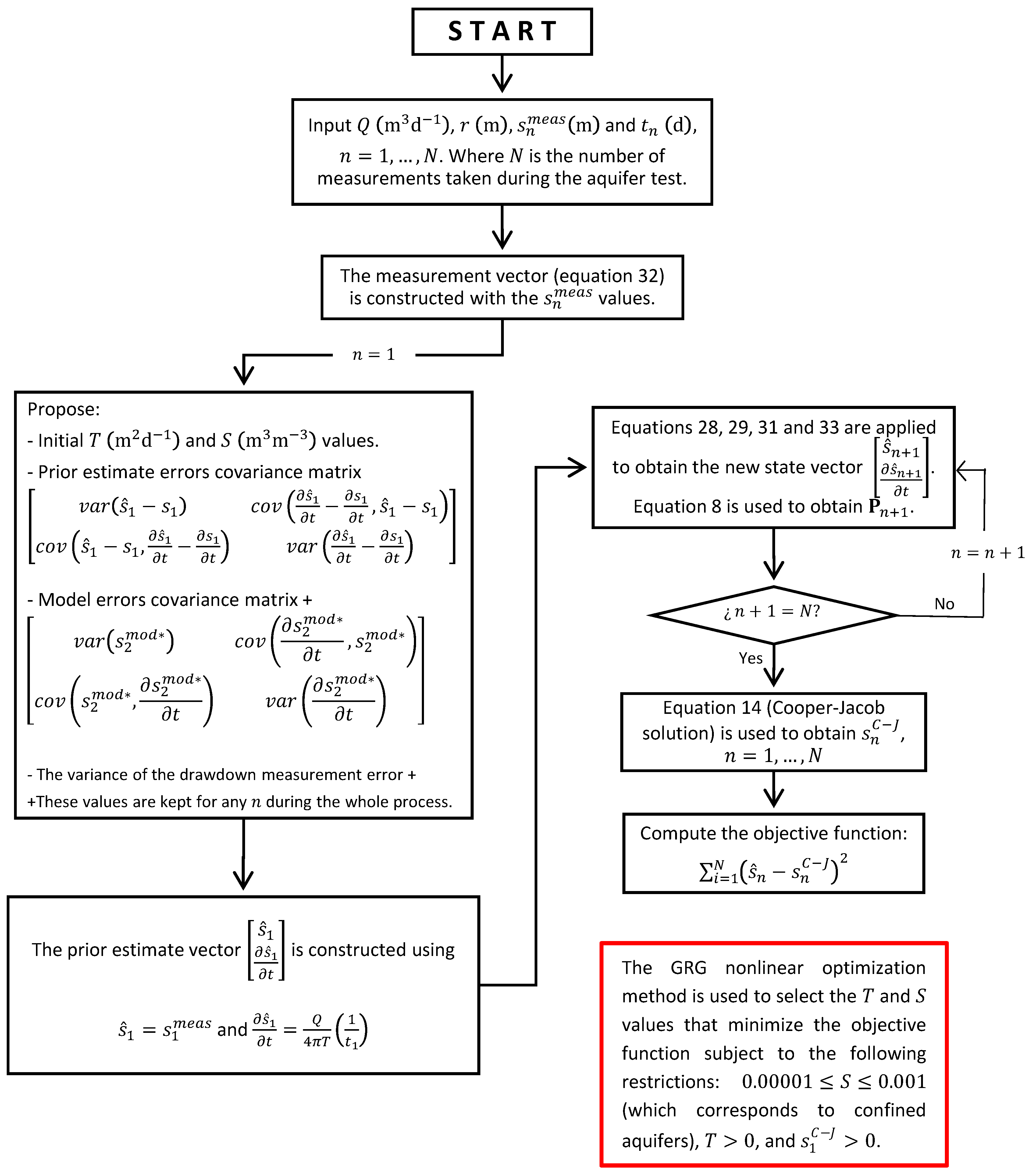
The full procedure is explained in the flowchart of Figure 1.

2.5. Case Study

The proposed approach was applied to confined-aquifer test data from two previously published cases. Theoretically, the assumptions employed in the development of the Cooper–Jacob solution are very approximate to real conditions for both cases.

(a)

The aquifer test “Oude Korendijk” presented in [34].

This aquifer test was conducted in the polder “Oude Korendijk”, south of Rotterdam, The Netherlands. The impermeable confining layer is composed of clay, peat, and clayey fine sand for the first 18 m below the surface. The aquifer (between 18 and 25 m below the surface) consists of coarse sand with some gravel. The base of the aquifer (considered impermeable) is formed by fine sandy and clayey sediments.

The well screen of the pumping well was installed over the whole thickness of the aquifer, and one piezometer with a depth of 20 m was placed at 30 m from it. Since other piezometers with a depth of 30 m showed a drawdown during pumping, it could be concluded that the clay layer between 25 and 27 m is not completely impermeable. For our purposes, however, we shall assume that all the water was derived from the aquifer between 18 and 25 m, and that the base is impermeable [34].

During the execution of the aquifer test, the data in

Table 1. Aquifer test data from the aquifer test “Oude Korendijk” [34].

Time after Pumping Started (min)	Drawdown (m)	Time after Pumping Started (min)	Drawdown (m)
0.10	0.040	18.00	0.680
0.25	0.080	27.00	0.742
0.50	0.130	33.00	0.753
0.70	0.180	41.00	0.779
1.00	0.230	48.00	0.793
1.40	0.280	59.00	0.819
1.90	0.330	80.00	0.855
2.33	0.360	95.00	0.873
2.80	0.390	139.00	0.915
3.36	0.420	181.00	0.935
4.00	0.450	245.00	0.966
5.35	0.500	300.00	0.990
6.80	0.540	360.00	1.007
8.30	0.570	480.00	1.050
8.70	0.580	600.00	1.053
10.00	0.600	728.00	1.072
13.10	0.640	830.00	1.088

were collected in the piezometer located 30 m from the pumping well, and the well was pumped at a constant discharge of $9.12{ \mathrm{L}}^1{\mathrm{s}}^{-1}$ $(\mathrm{or} 788{ \mathrm{m}}^3{\mathrm{d}}^{-1})$ for nearly 14 h.

(b)

The aquifer test of Todd and Mays corresponding to exercise 4.4.2 of [4].

This case study consists of an aquifer test in a well penetrating a confined aquifer that was pumped at a uniform rate of 2500 ${\mathrm{m}}^3{\mathrm{d}}^{-1}$. Time-drawdown data measured during the pumping period in an observation well 60 m away are presented in

Table 2. Aquifer test data from the aquifer test of Todd and Mays [4].

Time after Pumping Started (min)	Drawdown (m)	Time after Pumping Started (min)	Drawdown (m)
1	0.2	24	0.72
1.5	0.27	30	0.76
2	0.3	40	0.81
2.5	0.34	50	0.85
3	0.37	60	0.9
4	0.41	80	0.93
5	0.45	100	0.96
6	0.48	120	1
8	0.53	150	1.04
10	0.57	180	1.07
12	0.6	210	1.1
14	0.63	240	1.12
18	0.67

. In this case, there was no additional information about the aquifer conditions, and the constructive characteristics of the pumping and the observation well.

3. Results

For the implementation of the proposed procedure in the case studies, the following values were used:

-

Initial values: $T=100{ \mathrm{m}}^2{\mathrm{d}}^{-1}$ and $S=0.00001{ \mathrm{m}}^3{\mathrm{m}}^{-3}$.

-

The prior estimate errors covariance matrix $[\begin{array}{cc}0.25& 5\\ 5& 100\end{array}]$

-

The model errors covariance matrix $[\begin{array}{cc}0.0001& 0.001\\ 0.001& 0.1\end{array}]$

-

The variance of the drawdown measurement error (VDME) = 0.01 ${\mathrm{m}}^2$.

3.1. The Aquifer Test “Oude Korendijk”

To construct the prior estimate vector required in Equation (28), it is necessary to select initial estimates for the drawdown and the drawdown rates. The drawdown measured at time $t_1$ ($s_1^{meas}=0.040 \mathrm{m})$ was taken as the initial estimate for the drawdown (${\widehat{s}}_1$). The initial estimate for the drawdown rate was calculated with Equation (19), resulting in:

$$\frac{\partial {\widehat{s}}_1}{\partial t}=\frac{Q}{4\pi T}(\frac{1}{t_1})=\frac{788{ \mathrm{m}}^3{\mathrm{d}}^{-1} }{4\pi (100{ \mathrm{m}}^2{\mathrm{d}}^{-1})}(\frac{1}{\frac{0.10}{60\times 24} \mathrm{d}})=9029.81{ \mathrm{m}}^1{\mathrm{d}}^{-1}.$$

In this manner, the constructed prior estimate vector was $[\begin{array}{c}0.040\\ 9029.81\end{array}]$.

Once we had applied the GRG nonlinear optimization for the proposed procedure, $T=510.59{ \mathrm{m}}^2{\mathrm{d}}^{-1}$ and $S=0.000089{ \mathrm{m}}^3{\mathrm{m}}^{-3}$ were determined.

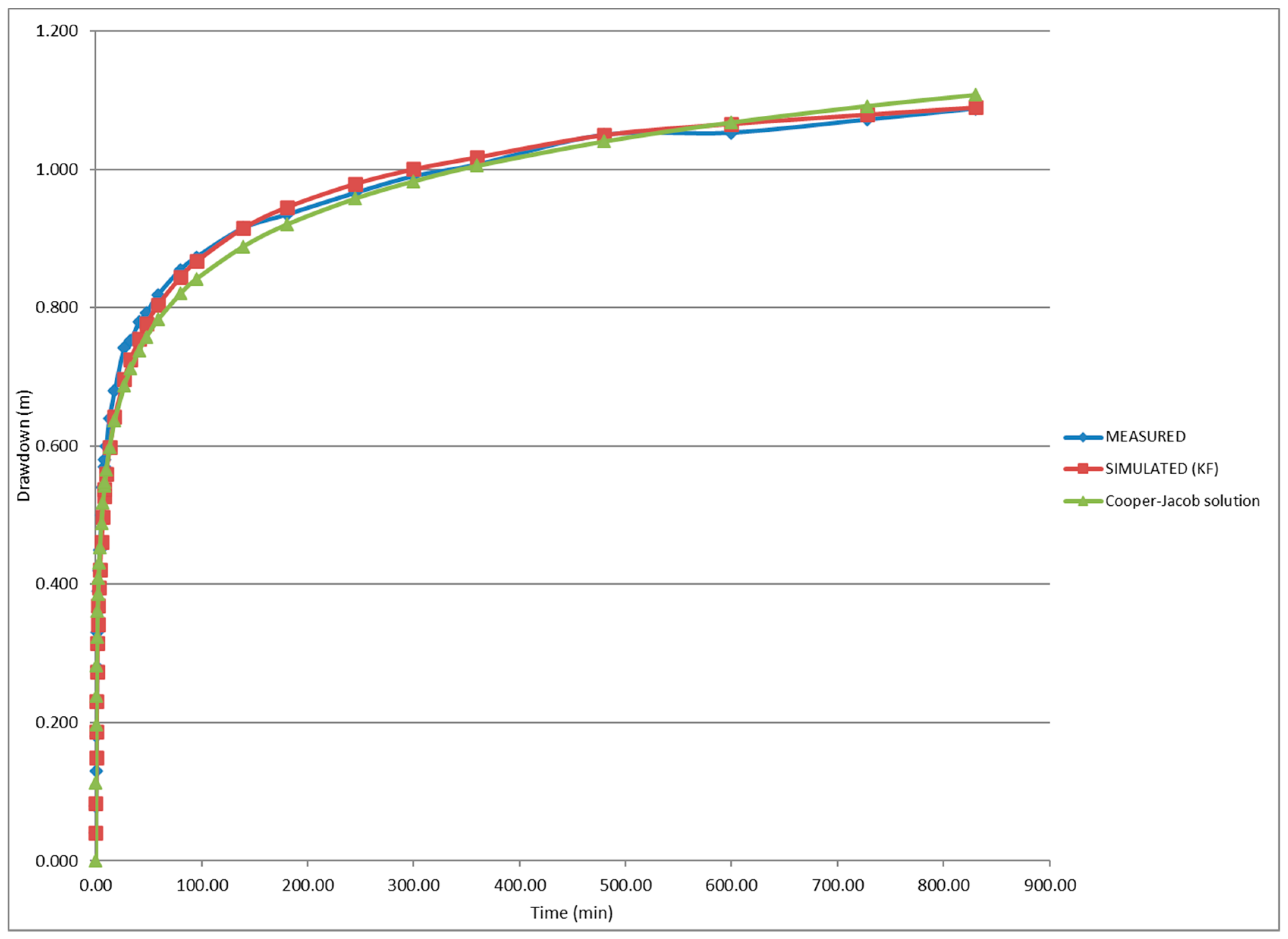
In Figure 2, a mismatch between the simulated drawdowns and the Cooper–Jacob solution before and after the 600 min point can be observed, although both follow the general evolution of the measured data.

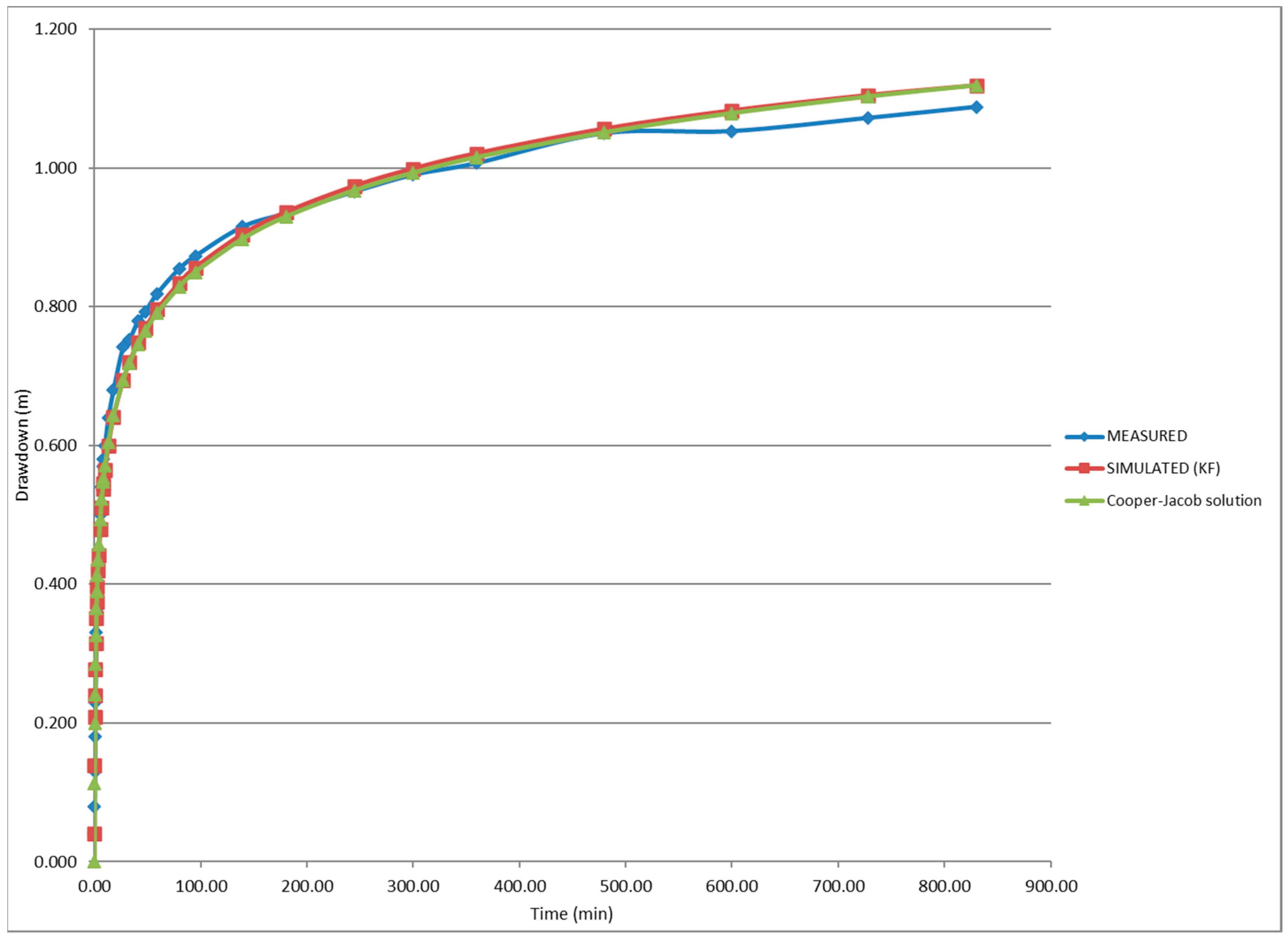
When using a VDME = 1.00 ${\mathrm{m}}^2$, $T=505.76{ \mathrm{m}}^2{\mathrm{d}}^{-1} \mathrm{and}$ $S=0.000088{ \mathrm{m}}^3{\mathrm{m}}^{-3}$ are obtained. The magnitude of this considered measurement error helps to filter the measurements in a manner that allows us to obtain a better adjustment between the simulated values and the Cooper–Jacob solution (Figure 3). However, simulated drawdowns and the Cooper–Jacob solution deviate significantly from the measurements for times greater than 500 min.

For comparison purposes, in

Table 3. Hydraulic parameters determined for data of the aquifer test “Oude Korendijk” using different interpretation procedures.

Parameter	Theis Procedure *	Cooper-Jacob Procedure *	Şen Procedure *	AquiferWin (Theis Solution)	KF-Based Proposed Procedure (VDME = 0.01 $m^2$)	KF-Based Proposed Procedure (VDME = 0.01 $m^2$)
$T ({\mathrm{m}}^2{\mathrm{d}}^{-1})$	342–418	375–401	342–420	480.67	510.59	505.76
$S ({\mathrm{m}}^3{\mathrm{m}}^{-3})$	0.00017	0.00022–0.00017	0.00016–0.0002	0.000112	0.000089	0.000088

* Values reported in [27].

are also presented the values for $T$ and $S$ reported in [27] obtained with traditional methods (Theis and Cooper–Jacob procedures) and using an adaptative pumping test analysis based on the Kalman filter (the Şen procedure); the results of using the software AquiferWin32 version 4.00 [16] are also included.

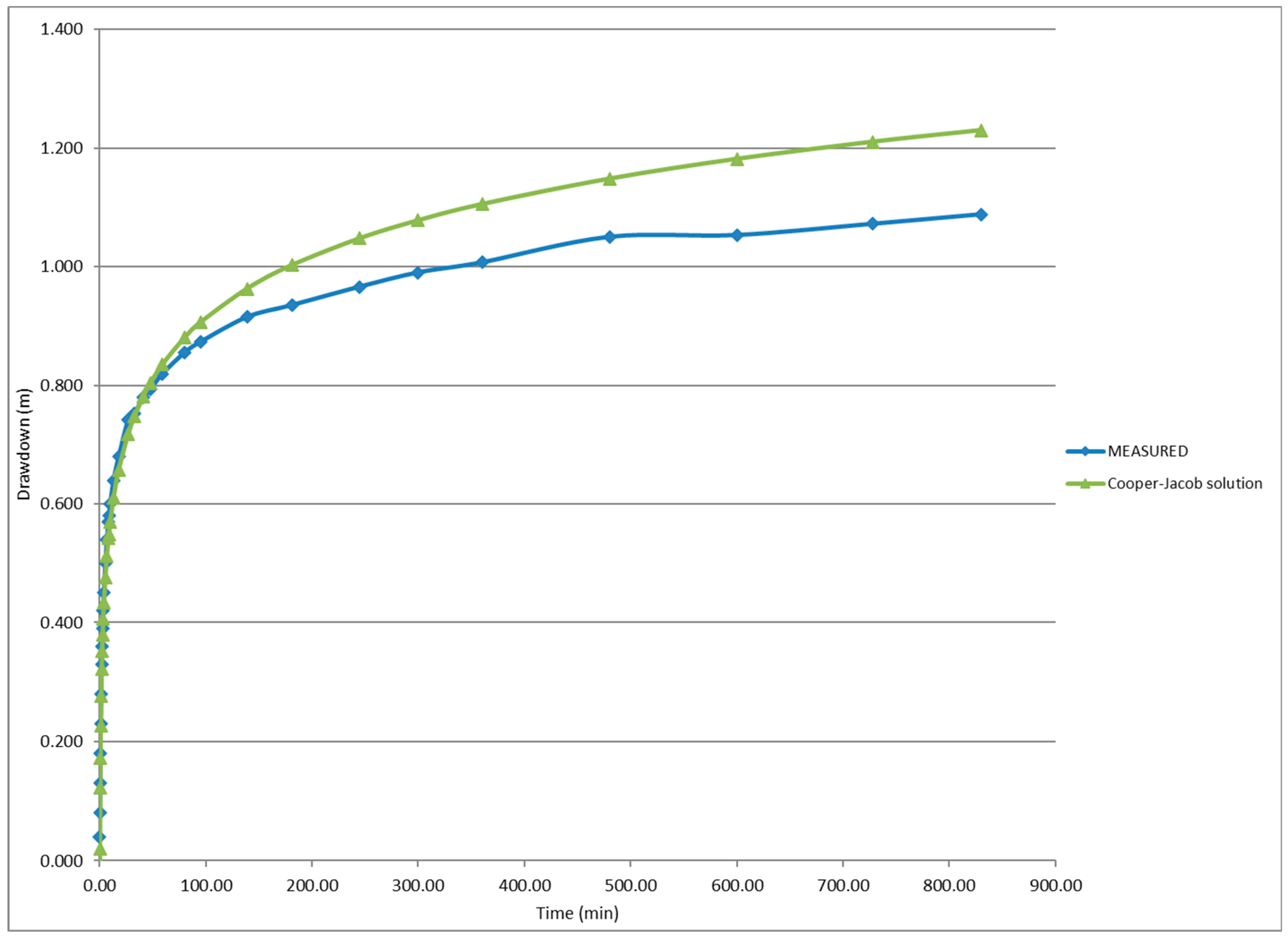
In Table 3, it can be observed that the values reported in [27] for $T$ and $S$ differ considerably from those found with the procedure proposed in this paper. When the former parameters are used to obtain drawdowns with the Cooper–Jacob solution, significant differences are obtained with respect to the measurements, especially for larger times. As an example, in Figure 4, the Cooper–Jacob solution for $T=420{ \mathrm{m}}^2{\mathrm{d}}^{-1} \mathrm{and}$ $S=0.00016{ \mathrm{m}}^3{\mathrm{m}}^{-3}$ is compared with the drawdown data of the aquifer test “Oude Korendijk”. A poor match is seen since the procedure for the selection of these hydraulic parameters assumed error-free measurements.

The plotting of measured drawdown data showed, from the initial moments of the aquifer test, significant deviations with respect to the estimates with the Cooper–Jacob solution using the $T$ and $S$ values obtained following the traditional and the adaptative methods. This result implies that these values are not representative of the actual aquifer conditions. When using the hydraulic parameters selected with the Kalman filter-based procedure, a best match between measured drawdowns and the Cooper–Jacob solution was obtained. Furthermore, increasing the value for the measurement errors produced a better adjustment between the Kalman filter estimates and the Cooper–Jacob solution; however, from 500 min after starting the aquifer test onwards, the measured drawdowns are consistently smaller than the estimates. These differences could reflect systematic errors for measurements, the non-compliance of the model assumptions, or a combination of both. Apparently, some considerable measurement errors occurred during the execution of the aquifer test, since the Kalman filter estimates and the Cooper–Jacob solution are more similar when the measurement uncertainties are increased in the proposed procedure. On the other hand, the smaller values of measured drawdowns for times greater than 500 min could reflect that some water is entering into the aquifer due to the permeability of the supposedly “confining” layers, as is stated in the description of this case study; in this case, one fundamental assumption of the selected model is not fulfilled.

3.2. The Aquifer Test of Todd and Mays

The prior estimate vector for this case study was constructed taking the drawdown measured at time $t_1$ ($s_1^{meas}=0.20 \mathrm{m})$ as the initial estimate for the drawdown (${\widehat{s}}_1$).

The initial estimate for the drawdown rate was calculated as:

$$\frac{\partial {\widehat{s}}_1}{\partial t}=\frac{Q}{4\pi T}(\frac{1}{t_1})=\frac{2500{ \mathrm{m}}^3{\mathrm{d}}^{-1} }{4\pi (1000{ \mathrm{m}}^2{\mathrm{d}}^{-1})}(\frac{1}{\frac{1}{60\times 24} \mathrm{d}})=2864.79{ \mathrm{m}}^1{\mathrm{d}}^{-1}$$

The prior estimate vector was then $[\begin{array}{c}0.20\\ 2864.79\end{array}]$.

Following the proposed procedure, $T=1180.43{ \mathrm{m}}^2{\mathrm{d}}^{-1}$ and $S=0.00017{ \mathrm{m}}^3{\mathrm{m}}^{-3}$ were determined.

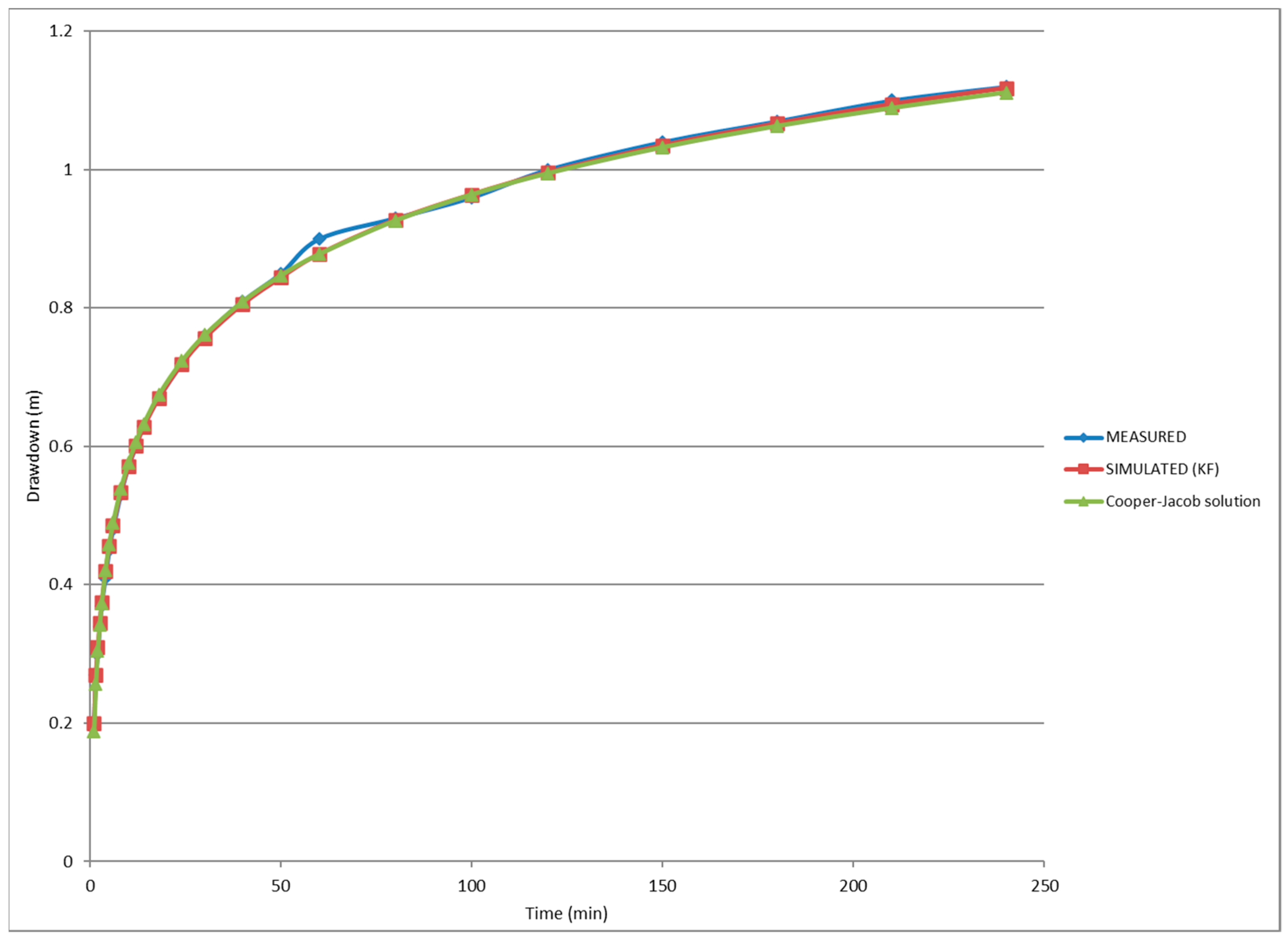
The Kalman filter estimates using these values for the hydraulic parameters are very similar to the measurements and the Cooper–Jacob solution (Figure 5), which indicates that the measurement and model errors are low for this aquifer test. The measurement taken at 60 min presents the largest error, but this is filtered during the simulation.

The hydraulic parameters for the different interpretations reported in

Table 4. Hydraulic parameters determined for data of the aquifer test of Todd using different interpretation procedures.

Parameter	Theis Procedure *	Cooper–Jacob Procedure *	AquiferWin (Theis Solution)	KF-Based Proposed Procedure (VDME = 0.01 $m^2$)
$T ({\mathrm{m}}^2{\mathrm{d}}^{-1})$	1110	1144	1138.17	1180.43
$S ({\mathrm{m}}^3{\mathrm{m}}^{-3})$	0.000206	0.000193	0.00019	0.00017

* Values reported in [4].

are by far more similar when compared to those corresponding to the “Oude Korendijk” case; this lower variability is related to the smaller measurement errors during the execution of the aquifer test and the high compliance of the model assumptions. For this reason, it was considered unnecessary to present the comparison between the measurements and the Cooper–Jacob solution for another pair of hydraulic parameters.

4. Discussion

The values of $T$ and $S$ obtained with the Kalman filter-based procedure were compared to those determined by other authors following previously developed approaches; the largest differences between these values were obtained for the case study with larger measurement and model errors. Following the proposed methodology for the interpretation of aquifer tests (filtering the model and measurement errors), the largest $T$ values and the smallest $S$ values were found for both case studies with respect to the methodologies that neglect these errors. According to the new values determined for these hydraulic parameters, water would flow easier, and the same amount of abstracted water would increase the drawdowns within the aquifer. Differences between the values of the hydraulic parameters for the different methods increase when measurement and model errors do the same.

For the aquifer test “Oude Korendijk”, the largest value determined for $T$ $(510.59{ \mathrm{m}}^2{\mathrm{d}}^{-1})$ is 49.29% larger than the smallest $(342{ \mathrm{m}}^2{\mathrm{d}}^{-1})$, while the largest value for $S$ $(0.00022{ \mathrm{m}}^3{\mathrm{m}}^{-3})$ is 150% larger than the smallest $(0.000088{ \mathrm{m}}^3{\mathrm{m}}^{-3})$. These results reflect significant measurement and model errors for the aquifer test; it is clear that even using an extremely large value of 1.00 ${\mathrm{m}}^2$ for the variance of the drawdown measurement error, the filtered data do not match the measured drawdowns, which reflects the considerable deviations in the aquifer conditions with respect to the proposed model.

For the case of the aquifer test of Todd and Mays, the largest value for $T$ $(1180{ \mathrm{m}}^2{\mathrm{d}}^{-1})$ is 6.34% larger than the smallest $(1110{ \mathrm{m}}^2{\mathrm{d}}^{-1})$, while the largest value for $S$ $(0.000206{ \mathrm{m}}^3{\mathrm{m}}^{-3})$ is 21.17% larger than the smallest $(0.00017{ \mathrm{m}}^3{\mathrm{m}}^{-3})$. In this case, measurement and model errors can be considered to be low, since a value of 0.01 ${\mathrm{m}}^2$ for the variance of the drawdown measurement error and the proposed values for the model errors covariance matrix helps to adequately filter the measured drawdowns.

These results show the relevance of the proposed procedure for the interpretation of aquifer tests, since it provides additional information about the compliance of the model assumptions and the quality of measured drawdown data.

With the proposed methodology, drawdowns and drawdown rates can be estimated at any time of the aquifer test with their respective estimate error variances, which could be useful in cases where some aquifer test data need to be determined, are missing or seem to be suspicious.

Future research could evaluate the confidence in the execution of an aquifer test by exploring optimization methods to quantify measurement and model errors. Future developments should also be made to obtain the estimate error variances of the determined hydraulic parameters.

5. Conclusions

The Kalman filter-based procedure proposed in this paper represents a new alternative for the interpretation of aquifer tests in confined aquifers considering model and measurement errors. It is based on the Cooper–Jacob solution due to its relatively simple implementation in the Kalman filter estimation method.

The existing methods for the interpretation of aquifer tests produce virtually the same hydraulic parameters when measurement and model errors are low; however, the differences between the determined values of $T$ and $S$ increase for large measurement errors, the non-compliance of the model assumptions, or a combination of both. Neglecting these errors could lead to determining values for the hydraulic parameters that do not adequately characterize the actual aquifer conditions.

One important advantage of the proposed Kalman filter-based procedure is that it can help to quantify the measurement errors during the execution of aquifer tests and/or identify significant deviations in the aquifer conditions with respect to the model assumptions; to complement this analysis, it is fundamental to provide a description of the execution of the aquifer test (including the techniques and instruments used to measure the flow rate and drawdowns), the hydrogeological framework including the hydrostratigraphic units and the constructive characteristics of the pumping and observation wells.

Furthermore, using the hydraulic parameters selected with this procedure produces a best match between the measured drawdowns and the Cooper–Jacob solution; this result shows that the determined $T$ and $S$ values calibrate more accurately the selected flow model.

References

- Konikow, L.F.; Glynn, P.D. Modeling Groundwater Flow and Quality. In Essentials of Medical Geology, 2nd ed.; Selinus, O., Ed.; Springer: Dordrecht, Germany, 2013; Volume 1, pp. 727–753. [Google Scholar] [CrossRef]
- Freeze, A.; Cherry, J. Groundwater, 1st ed.; Prentice-Hall: Hoboken, NJ, USA, 1979. [Google Scholar]
- Moore, J.E. Contribution of groundwater modeling to planning. J. Hydrol. 1979, 43, 121–128. [Google Scholar] [CrossRef]
- Todd, D.K.; Mays, L.W. Groundwater Hydrology, 3rd ed.; John Wiley & Sons: Hoboken, NJ, USA, 2004. [Google Scholar]
- Fetter, C.W. Applied Hydrogeology, 4th ed.; Prentice Hall: Upper Saddle River, NJ, USA, 2001. [Google Scholar]
- Theis, C.V. The relationship between the lowering of the piezometric surface and the rate and duration of discharge of a well using ground-water storage. Trans. Am. Geophys. Union 1935, 16, 519–524. [Google Scholar] [CrossRef]
- Cooper, H.H., Jr.; Jacob, C.E. A generalized graphical method for evaluating formation constants and summarizing well-field history. Trans. Am. Geophys. Union 1946, 27, 526–534. [Google Scholar] [CrossRef]
- Neuman, S.P. Effect of partial penetration on flow in unconfined aquifers considering delayed gravity response. Water Resour. Res. 1974, 10, 303–312. [Google Scholar] [CrossRef]
- Moench, A.F. Flow to a well of finite diameter in a homogeneous, anisotropic water table aquifer. Water Resour. Res. 1997, 33, 1397–1407. [Google Scholar] [CrossRef]
- Hantush, M.S.; Jacob, C.E. Non-steady radial flow in an infinite leaky aquifer. Trans. Am. Geophys. Union 1955, 36, 95–100. [Google Scholar] [CrossRef]
- Hantush, M.S. Modification of the theory of leaky aquifers. J. Geophys. Res. 1960, 65, 3713–3725. [Google Scholar] [CrossRef]
- Neuman, S.P.; Witherspoon, P.A. Field determination of the hydraulic properties of leaky multiple aquifer systems. Water Resour. Res. 1972, 8, 1284–1298. [Google Scholar] [CrossRef] [Green Version]
- Moench, A.F. Double-porosity models for a fissured groundwater reservoir with fracture skin. Water Resour. Res. 1984, 20, 831–846. [Google Scholar] [CrossRef]
- Barker, J.A. A generalized radial flow model for hydraulic tests in fractured rock. Water Resour. Res. 1988, 24, 1796–1804. [Google Scholar] [CrossRef] [Green Version]
- Rumbaugh, J.O.; Rumbaugh, D.B. Guide to Using Aquifer Win32; Environmental Simulations, Inc.: Reinholds, PA, USA, 1997. [Google Scholar]
- Waterloo Hydrogeologic AquiferTest Pro 10.0, Pumping and Slug Test Analysis, Interpretation and Visualization Software. 2020. User’s manual. Available online: https://www.waterloohydrogeologic.com/wp-content/uploads/PDFs/aquifertest/AquiferTest_Users_Manual.pdf (accessed on 28 December 2021).
- Duffield, G.M. AQTESOLV (AQuifer TESt SOLVer) for Windows Version 4.5 User’s Guide; HydroSOLVE, Inc.: Reston, VA, USA, 2007; Available online: http://www.aqtesolv.com/download/aqtw20070719.pdf (accessed on 28 December 2021).
- Sindalovskiy, L.N. Analytical Modeling of Aquifer Tests and Well Systems (ANSDIMAT Software Guide); Nauka: Sankt-Petersburg, Russia, 2014; Available online: http://ansdimat.com/help/source/ (accessed on 28 December 2021).
- Boonstra, J.; Kselik, R.A.L. SATEM 2002: Software for Aquifer Test Evaluation. International Institute for Land Reclamation and Improvement/ILRI; AA: Wageningen, The Netherlands, 2001; 148p, Available online: https://edepot.wur.nl/82326 (accessed on 28 December 2021).
- Rathod, K.S.; Rushton, K.R. Interpretation of pumping from a two-zone layered aquifer using a numerical model. Ground Water 1991, 29, 499–509. [Google Scholar] [CrossRef]
- Rushton, K.R. Groundwater Hydrology: Conceptual and Computational Models, 1st ed.; John Wiley & Sons: West Sussex, UK, 2003. [Google Scholar]
- Moradkhani, H.; Sorooshian, S.; Gupta, H.V.; Hauser, P.R. Dual state–parameter estimation of hydrological models using ensemble Kalman filter. Adv. Water Res. 2005, 28, 135–147. [Google Scholar] [CrossRef] [Green Version]
- Andricevic, R. Cost-effective network design for groundwater flow monitoring. Stochastic Hydrol. Hydraul. 1990, 4, 27–41. [Google Scholar] [CrossRef]
- Zhou, H.; Gómez-Hernández, J.J.; Hendricks-Franssen, H.J.; Li, L. An approach to handling non-Gaussianity of parameters and state variables in ensemble Kalman filtering. Adv. Water Resour. 2011, 34, 844–864. [Google Scholar] [CrossRef] [Green Version]
- Haught, J.; Hopkinson, K.; Stuckey, N.; Dop, M.; Stirling, A. A Kalman filter-based prediction system for better network context-awarenesss. In Proceedings of the 2010 Winter Simulation Conference, Baltimore, MI, USA, 5–8 December 2010; pp. 2927–2934. Available online: https://www.informs-sim.org/wsc10papers/271.pdf (accessed on 15 December 2021).
- Clark, M.P.; Rupp, D.; Woods, R.A.; Zheng, X.; Ibbitt, R.P.; Slater, A.G.; Schmidt, J.; Uddstrom, M. Hydrological data assimilation with the ensemble Kalman filter: Use of streamflow observations to update states in a distributed hydrological model. Adv. Water Resour. 2008, 31, 1309–1324. [Google Scholar] [CrossRef]
- Júnez-Ferreira, H.E.; González-Trinidad, J.; Júnez-Ferreira, C.A.; Robles Rovelo, C.O.; Herrera, G.; Olmos-Trujillo, E.; Bautista-Capetillo, C.; Contreras Rodríguez, A.R.; Pacheco-Guerrero, A.I. Implementation of the Kalman Filter for a Geostatistical Bivariate Spatiotemporal Estimation of Hydraulic Conductivity in Aquifers. Water 2011, 12, 3136. [Google Scholar] [CrossRef]
- Şen, Z. Adaptive pumping test analysis. J. Hydrol. 1984, 74, 259–270. [Google Scholar] [CrossRef]
- Leng, C.H.; Yeh, H.D. Aquifer parameter identification using the extended Kalman filter. Water Resour. Res. 2003, 39, 1–16. [Google Scholar] [CrossRef]
- Ostad-Ali-Askar, K.; Shayannejad, M.; Ghorbanizadeh-Kharazi, H. Artificial Neural Network for Modeling Nitrate Pollution of Groundwater in Marginal Area of Zayandeh-rood River, Isfahan, Iran. KSCE J. Civ. Eng. 2017, 21, 134–140. [Google Scholar] [CrossRef]
- Kalman, R.E. A New Approach to Linear Filtering and Prediction Problems. J. Basic Eng. 1960, 82, 35–45. [Google Scholar] [CrossRef] [Green Version]
- Lasdon, L.S.; Fox, R.S.; Ratner, M.W. Nonlinear optimization using the generalized reduced gradient method. Revue française d’automatique, informatique, recherche opérationnelle. Rech. Opérationnelle 1974, 8, 73–103. [Google Scholar] [CrossRef] [Green Version]
- Microsoft Corporation. 2022. Microsoft Excel Version 2201. Available online: https://office.microsoft.com/excel (accessed on 26 January 2022).
- Kruseman, G.P.; de Ridder, N.A. Analysis and Evaluation of Pumping Test Data, 2nd ed.; Publication 47; International Institute for Land Reclamation and Improvement: Wageningen, The Netherlands, 1994. [Google Scholar]
Figure 1.
Flow chart of the Kalman filter-based procedure to interpret aquifer tests.
Figure 2.
Comparison between the measured drawdowns, simulated with the Kalman Filter (VDME = 0.01 ) and the Cooper–Jacob solution (the aquifer test “Oude Korendijk”).
Figure 3.
Comparison between the measured drawdowns, simulated with the Kalman filter (VDME = 1.00 ), and the Cooper–Jacob solution (the aquifer test “Oude Korendijk”).
Figure 4.
Comparison between the measured drawdowns and the Cooper–Jacob solution using (the aquifer test “Oude Korendijk”).
Figure 5.
Comparison between the measured drawdowns, simulated with the Kalman filter (VDME = 0.01 ) and the Cooper–Jacob solution (the aquifer test of Todd and Mays).