Assessing the Effect of Land-Use and Land-Cover Changes on Discharge and Sediment Yield in a Rural Coal-Mine Dominated Watershed in Kentucky, USA

Abstract

The Appalachian Mountain region of eastern Kentucky is unique and contains high proportions of forestland along with coal and natural gas depositaries. Landscape changes due to extreme mining activities can eventually threaten the downstream ecosystems, including soil and water quality, resulting in excessive runoff and sedimentation. The purpose of this study is to assess the impacts of land-use and land-cover (LULC) changes in streamflow and sediment yield in Yellow Creek Watershed, Kentucky, USA, between 1992 and 2016. LULC, digital elevation model, soil, and weather data were inputted into the Soil and Water Assessment Tool (SWAT) to simulate discharge and sediment yield. The model output was evaluated on several statistical parameters, such as the Nash-Sutcliffe efficiency coefficient (NSE), RMSE-observations standard deviation ratio (RSR), percent bias (PBIAS), and the coefficient of determination (R²). In addition, two indices, P-factor and R-factor, were used to measure the prediction uncertainty. The calibrated model showed an increase in surface runoff and sediment yield due to changes in LULC in the Yellow Creek Watershed. The results provided important insights for studying water management strategies to make more informed land management decisions and adaptive practices.

1. Introduction

Land-use and land-cover (hereafter LULC) change is a phenomenon that has been taking place since the beginning of humankind. It has long been considered a factor affecting the global environment [1,2]. Numerous studies over the past decade have highlighted the role of LULC change on various aspects of the environment, such as hydrological response [3,4,5], climate change [6,7,8], ecosystem services [9,10], and food security [11,12]. Among the studied impacts of LULC change, hydrological responses and accompanying factors, such as water quality and quantity, have received a great deal of attention. The complexities in the LULC change process and the associated hydrological cycle vary across geographic regions [1]. Changes in LULC in the watershed alter hydrological responses, including increased runoff, high streamflow, soil erosion, and inferior water quality [4,5,13,14]. Moreover, studies have shown wide variations in hydrological responses due to variations in watershed characteristics. This highlights the importance of LULC change impact on watershed levels, which is unique to the region itself.

Various anthropogenic activities have played an important role in landscape changes in the Appalachian Mountains region. Surface mining has been one of the major activities since World War II, resulting in a significant alteration in the mountain landscapes with the transformation of native forests and their associated soils into heavily disturbed mine lands [15,16,17]. The “Surface Mining Control and Reclamation Act of 1977” details the effects of surface mining on the landscape, including soil erosion and landslides, flooding, water contamination, and habitat destruction [18]. Furthermore, research has demonstrated the hydrologic effects of mining on Appalachian landscapes, including increased peak flows at newly mined watersheds in response to strong storm events, increased subsurface void space, and increased base flows [15,16,19].

It has become necessary to study the temporal and spatial variations in hydrological balance and to understand the mechanisms of influence behind LULC change impacts. However, it is impossible to measure every component of the hydrological system due mainly to watershed heterogeneity and inadequate measuring tools [20]. Hydrological models can assist in overcoming these constraints by extrapolating information to the watershed scale from available data in both time and space [21]. The Soil and Watershed Assessment Tool (SWAT) is the most frequently used hydrological model, evaluated across a broad range of watershed scales and environmental conditions throughout the world [22,23,24]. It can simulate the quantity and quality of surface and groundwater and predict the impact of land management practices on water, sediment, and agricultural chemical yields in large complex watersheds with heterogeneous soils, land use, and management conditions over a long period [22]. It requires specific information about weather, soil properties, topography, vegetation, and land management practices in the watershed to model the physical process associated with water movement, sediment movement, crop growth, and nutrient cycling [22,23].

In the United States, SWAT is increasingly being used to study in-stream processes [25,26], climate change impact [27,28,29], the impact of LULC changes [30,31], sediment loss and transport [32,33,34], the impact of best management practices [35,36,37], and other water use and water quality applications [38,39,40]. SWAT has also emerged in other regions, as shown by various studies published in multiple journals [4,14,41,42,43,44]. However, a hydrological model, such as SWAT, has much potential that remains to be fully utilized for the Appalachian Mountains region, particularly in Kentucky. To date, very few modeling studies that employ SWAT have been undertaken in Kentucky; in one study, Spruill et al. [45] simulated the discharge using the SWAT model in a small watershed in central Kentucky. They found the model effective for describing monthly runoff in the karst-influenced watershed. Chattopadhyay et al. [46] evaluated the potential impacts of climate change on the hydrologic process in the Kentucky River basin using SWAT. Modeled future scenarios reported an increase in monthly surface runoff, evapotranspiration, and water yield, resulting in hydrological drought.

Considering the void that exists in the literature, this study provides a case study from the Yellow Creek Watershed, a small critical watershed in eastern Kentucky that has been heavily impacted by coal-mining activities but supports local livelihoods and the ecosystem within and around the Appalachian Mountains region. The purpose of this study is to assess the impact of LULC changes on streamflow and sediment yield between 1992 and 2016. The Yellow Creek Watershed is particularly of interest to this study due to past and ongoing surface mining and reclamation activities as a major LULC change in the region (See Figure A1: Coal mine areas in and outside of the watershed). The availability of long-term observed discharge and sediment data, as well as the quality of da-ta available, have also been considered.

2. Materials and Methods

2.1. Description of the Study Region

The Yellow Creek Watershed falls within the Upper Cumberland River basin. The watershed is primarily located in Bell County, Kentucky, but extends into Claiborne County, Tennessee. The outlet of this watershed corresponds to the point where a monitoring station (USGS 03402000) is installed, which is at Yellow Creek near Middlesboro (latitude: 36°40′05″, longitude: 83°41′19″) (Figure 1). From the outlet, it derives a catchment area of 157.18 m². Except for the broad, alleviated valley of Yellow Creek at Middlesboro, most of the watershed is located in the rugged mountainous region with an elevation of 335 m to 960 m above sea level. The nearest United States Weather Bureau station is located at Middlesboro, at 358 m.a.s.l elevation. During the 1987–2016 period, the mean annual precipitation was 1283.64 mm. The mean annual temperature was 13.4 °C, with a mean winter minimum of −3 °C and a mean summer maximum of 24 °C. According to the Cropscape-Cropland data of 2016, the watershed was majority forested (76.14%), followed by urban (15.37%), pasture (6.11%), and barren land (2.0%).

2.2. The SWAT Model

The SWAT model is a physically based, watershed-scale simulation model jointly developed by the USDA Agricultural Research Service and Texas A&M AgriLife Research, part of the Texas A&M University System [22,23]. In SWAT, a watershed is divided into a number of sub-watersheds or sub-basins, which are further divided into hydrologic response units (HRUs) [23,47]. HRUs are lumped areas within the sub-basin that are comprised of unique land cover, soil, and slope. The model estimates relevant hydrologic components such as evapotranspiration, surface runoff, groundwater flow, and sediment yield for each HRU [23]. The hydrologic cycle simulated by SWAT is based on the water balance equation [23,47]:

$$SWt=SW0+ {\displaystyle \sum }_{i=1}^t{(R}_{\mathit{day}}-Q_{\mathit{surf}}-E_a-W_{\mathit{seep}}-Q_{\mathit{gw}})$$

(1)

where SW_t is the final soil water content on day i, SW₀ is the initial soil water content on day i, t is the time in days, R_day is the amount of rainfall on day i, Q_surf is the amount of surface runoff on day i, E_a is the amount of evapotranspiration on day i, W_seep is the amount of water entering the vadose zone from the soil profile on day i, and Q_gw is the amount of base flow or return flow on day i.

The surface runoff was estimated by using the United States Department of Agriculture (USDA) Soil Conservation Services (SCS) runoff curve number (CN) approach [22,23,48]. The CN is the function of land use, soil permeability, and antecedent soil moisture condition. The SCS equation [48] is:

$$Q_{\mathit{surf}}=\frac{{(R}_{\mathit{day}}-I_a{)}^2}{{(R}_{\mathrm{day}}{+I}_a+S)}$$

(2)

where Q_surf is the accumulated runoff or rainfall access, R_day is the rainfall depth of the day (mm H₂O), I_a is the initial abstractions, which includes surface storage, interception and infiltration prior to runoff (mm H₂O), and S is the retention parameter (mm H₂O). The retention parameter (S) is dependent spatially to changes in soils, land use, management, and slope, and temporarily to changes in soil water content [23]. The retention parameter (S) [23] is given by the equation

$$S=25.4\times \left(\frac{1000}{\mathit{CN}}-10\right)$$

(3)

where CN is the curve number for the day. The initial abstraction, I_a, is usually approximated as 0.2S, so equation 2 can be rewritten as

$$Q_{\mathit{surf}}=\frac{{(R}_{\mathrm{day}}-{0.2S)}^2}{{(R}_{\mathit{day}}+0.8S)}$$

(4)

The SWAT offers three methods to estimate potential evapotranspiration (PET): the Penman-Monteith method, the Priestley-Taylor method, and the Hargreaves method [23]. In our study, PET was estimated using the Penman/Monteith method, which requires solar radiation, air temperature, relative humidity, and wind speed as inputs. The Penman-Monteith equation [49] is

$$\lambda E=\frac{\Delta \left(H_{\mathit{net}}-G)+{\rho }_{\mathit{air}}·C_p·\right(e_z^0-e_z)/r_a}{\Delta +\gamma ·(1+r_c/r_a)}$$

where $\lambda E$ is the latent heat flux density (MJ m⁻² d⁻¹), E is the depth rate evaporation (mm d⁻¹), $\Delta$ is the slope of the saturation vapor pressure-temperature curve, de/dT (kPa °C^–1), H_net is the net radiation (MJ m⁻² d⁻¹), G is the heat flux density to the ground (MJ m⁻² d⁻¹), ${\rho }_{\mathit{air}}$ is the air density (kg m⁻³), c_p is the specific heat at constant pressure (MJ kg⁻¹ °C⁻¹), $e_z^0$ is the saturation vapor pressure of air at height z (kPa), $e_z$ is the water vapor pressure of air at height z (kPa), $\gamma$ is the psychometric constant (kPa °C⁻¹), $r_c$ is the plant canopy resistance (s m⁻¹), and $r_a$ is the diffusion resistance of the air layer (aerodynamic resistance) (s m⁻¹) [23]. Upon determination of PET, the actual evapotranspiration (ET) was calculated with the method similar to that suggested by Richtie [50].

The sediment component for each HRU was calculated using the modified universal soil loss equation (MUSLE). The MUSLE [51] is

$$\mathit{sed}=11.88·{{(Q}_{\mathit{surf}}·q_{\mathit{peak}}·{\mathit{area}}_{\mathit{hru}})}^{0.56}·K_{\mathit{USLE}}·C_{\mathit{USLE}}·P_{\mathit{USLE}}·{\mathit{LS}}_{\mathit{USLE}}·\mathit{CFRG}$$

(5)

where sed is the sediment yield on a given day (metric tons), Q_surf is the surface runoff volume (mm H₂O/ha), q_peak is the peak runoff rate (m³/s), area_hru is the area of HRU (ha), K_USLE is the USLE soil erodibility factor (0.013 metric ton m² hr/m³-metric ton cm), C_USLE is the USLE cover and management factor, P_USLE is the USLE support practice factor, LS_USLE is the USLE topographic factor, and CFRG is the coarse fragment factor. More details on SWAT can be found in the Soil and Water Assessment Tool theoretical documentation version 2009 (https://swat.tamu.edu/docs/, accessed on 20 December 2020) [22,23].

2.3. SWAT Input Data

2.3.1. Spatial Data

The spatial data used in SWAT for this study included Digital Elevation Model (DEM), soil and LULC data (Figure 2). DEM (30 m × 30 m resolution) was downloaded from the United States Geological Survey (USGS) at the National Map Viewer website. LULC data were obtained from the National Land Cover Database (NLCD) and CropScape-Cropland Data layer website. Soil data was downloaded from Soil Survey Geographic Database (SSURGO) at the Web Soil Survey website.

2.3.2. Hydro-Climatic Data

Table 1. Input data for the SWAT model.

Data	Date	Resolution	Source (Date Accessed: December 2020)
DEM	2018	30 m × 30 m	https://apps.nationalmap.gov/downloader/#/
Soil	2020	30 m × 30 m	https://websoilsurvey.nrcs.usda.gov/
LULC	1992, 2016	30 m × 30 m	https://www.mrlc.gov/data/, https://nassgeodata.gmu.edu/CropScape/
Precipitation and Temperature	1987–2016	4 km	(https://prism.oregonstate.edu/)
Wind, Relative humidity, and Solar radiation	1987–2016	0.25° × 0.25°	SWAT weather generator
Discharge	1990–2004	Observed	https://waterdata.usgs.gov/
Sediment	1990–2004	Observed/ LOADEST Simulated	https://waterdata.usgs.gov/

highlights the source and description of the data used in the SWAT model. The weather data was downloaded from PRISM Climate Group, which includes maximum and minimum temperature and precipitation. Wind speed, relative humidity, and solar radiation were simulated for the nearest weather station using the weather generator in SWAT. Monthly discharge (1987–2004) and sediment data (1987–1992) were obtained from the gauging station (USGS 03402000) at the outlet of the watershed. Since sediment data was only available for parts of the simulation periods (until 1992), we used a LOAD Estimator (LOADEST) to simulate sediment data to match the period with discharge (1987–2004).

The LOADEST is a FORTRAN-based model developed by the U.S. Geological Survey [52] to estimate the constituent loads in streams and rivers given a time series of stream flows, additional data variables, and constituent concentrations. It uses a regression model to estimate the constituent loads. Streamflow, the time factor, and the user-specified variables are the independent variables of the regression model which is used to estimate load over the user’s specified time interval. The regression model is used to estimate mean load and the statistical properties: standard errors and 95 percent confidence interval on a monthly basis.

LOADEST uses three statistical estimation methods for the calibration [52]. The first two methods, adjusted maximum likelihood estimation (AMLE) and maximum likelihood estimation (MLE), are useful when a model error (residuals) is normally distributed, whereas the third method, least absolute deviation (LAD), is useful when residuals are not normally distributed. The valuable information inside the LOADEST output, like diagnostic tests and warnings, helps users select the appropriate estimation method and interpret the estimated loads. The stream flows and their constituent are used to calibrate LOADEST to determine the best-preloaded models inside the LOADEST for load estimating.

2.4. SWAT Model Setup

ArcSWAT 2012, an ArcGIS extension and interface for SWAT, was used to simulate the SWAT model. ArcSWAT interface is a public domain software, and as such may be used freely [47]. ArcSWAT extension for ArcGIS and documentation are available as downloads (https://swat.tamu.edu/software/arcswat/ accessed on 20 December 2020). Based on ArcSWAT, the SWAT model data preparation is characterized by three modules: (1) the SWAT Watershed Delineator, which allows the users to discretize the watershed and sub-watersheds using the data derived from the digital elevation model (DEM); (2) the SWAT HRU Analysis Tool, which combines data derived from LULC, soil characteristics, and slope variations to discretize the HRUs; and (3) the SWAT Input Editor, which allows the user to create an input database and modify various model parameters.

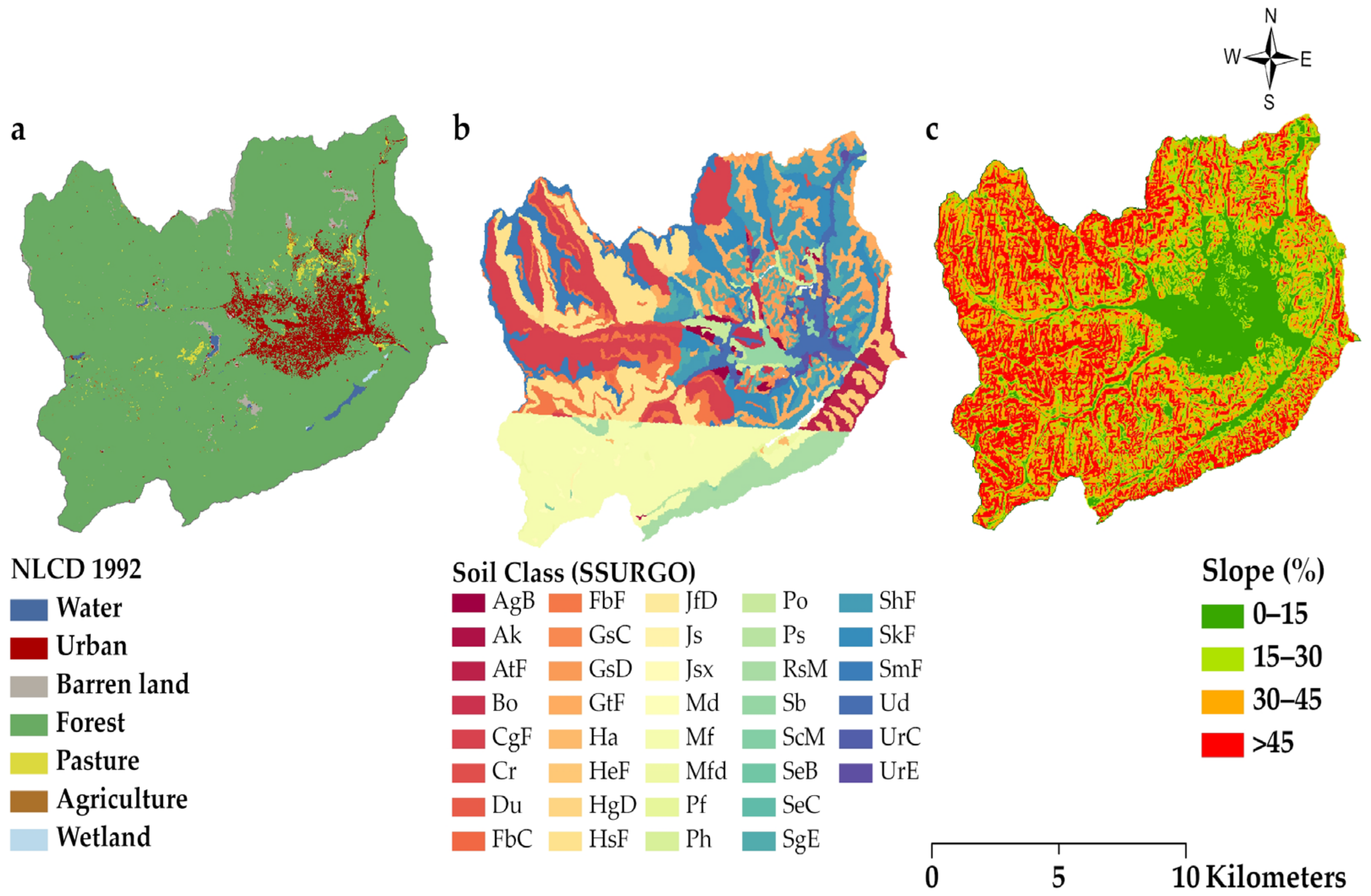
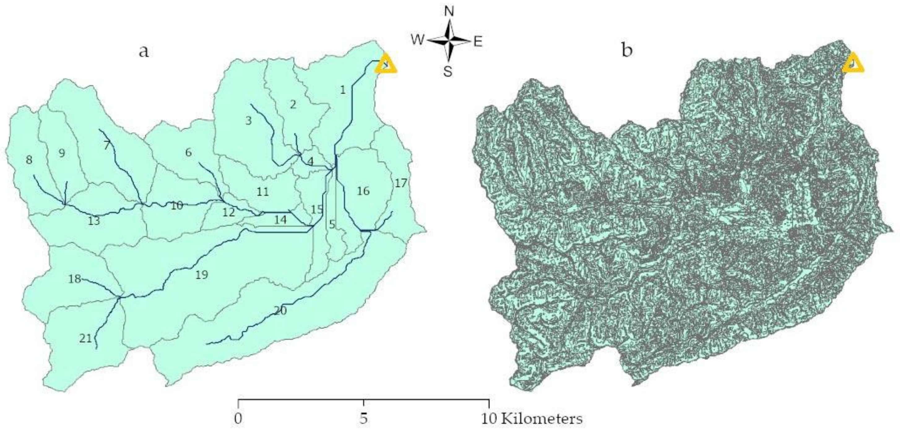
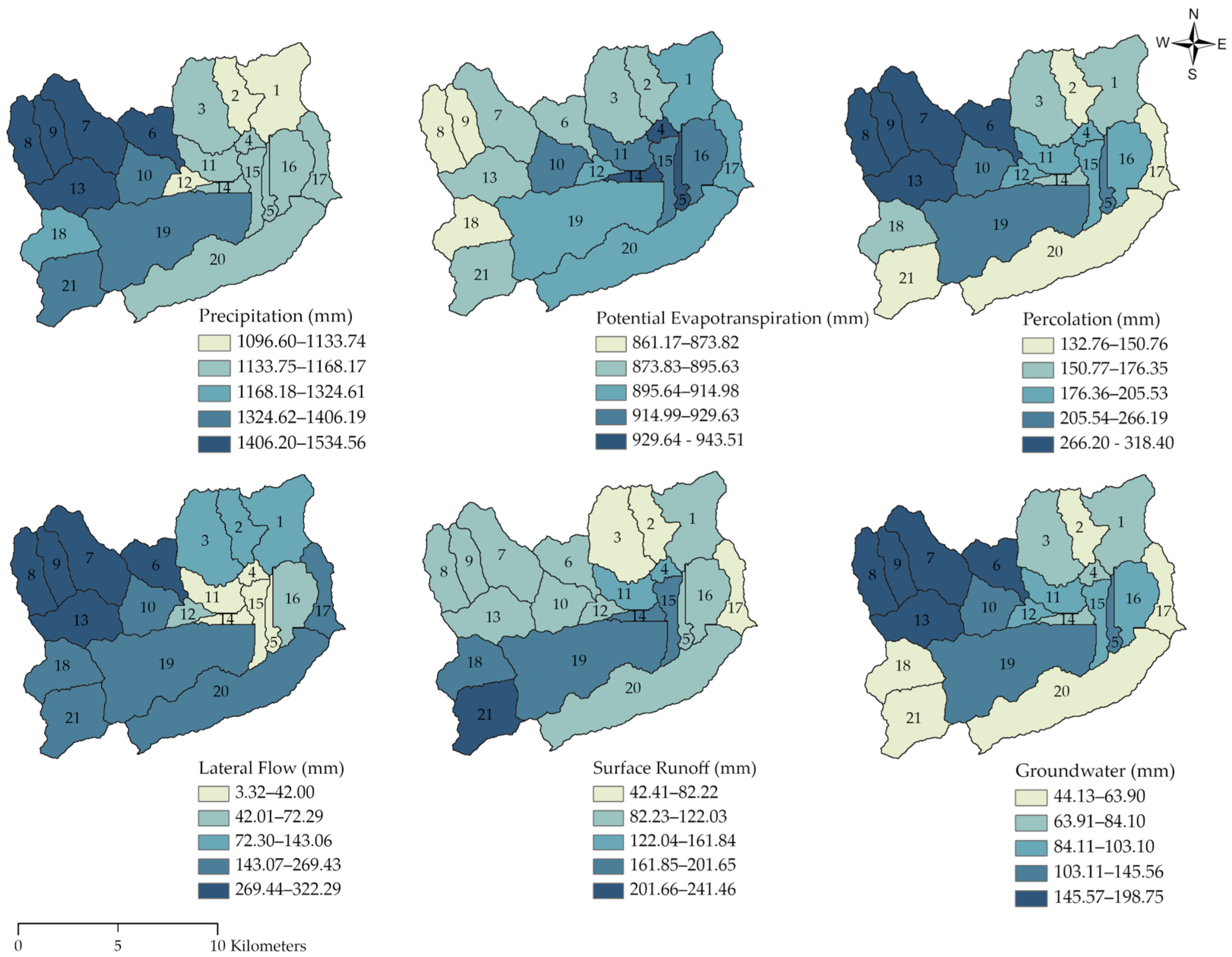
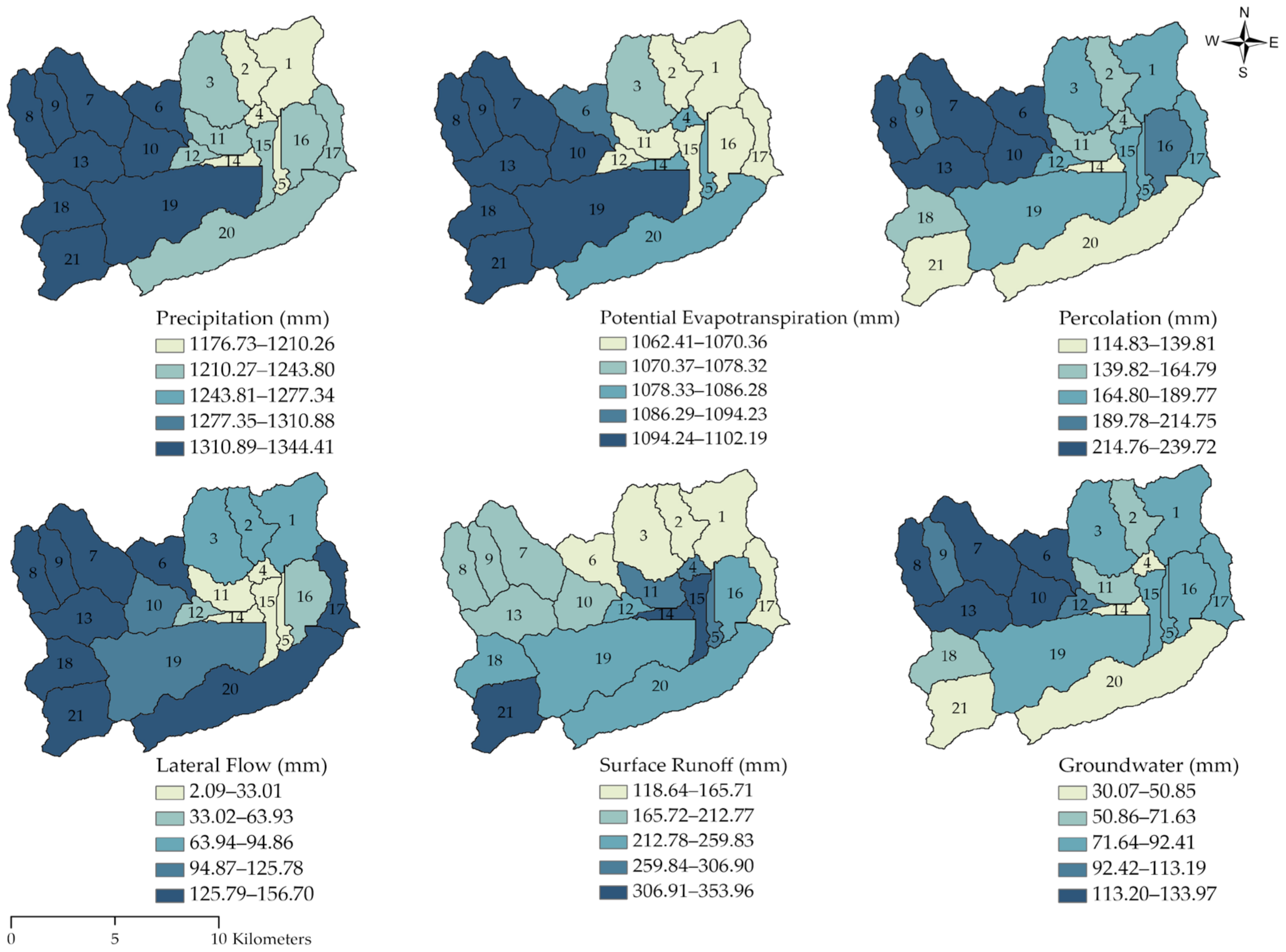
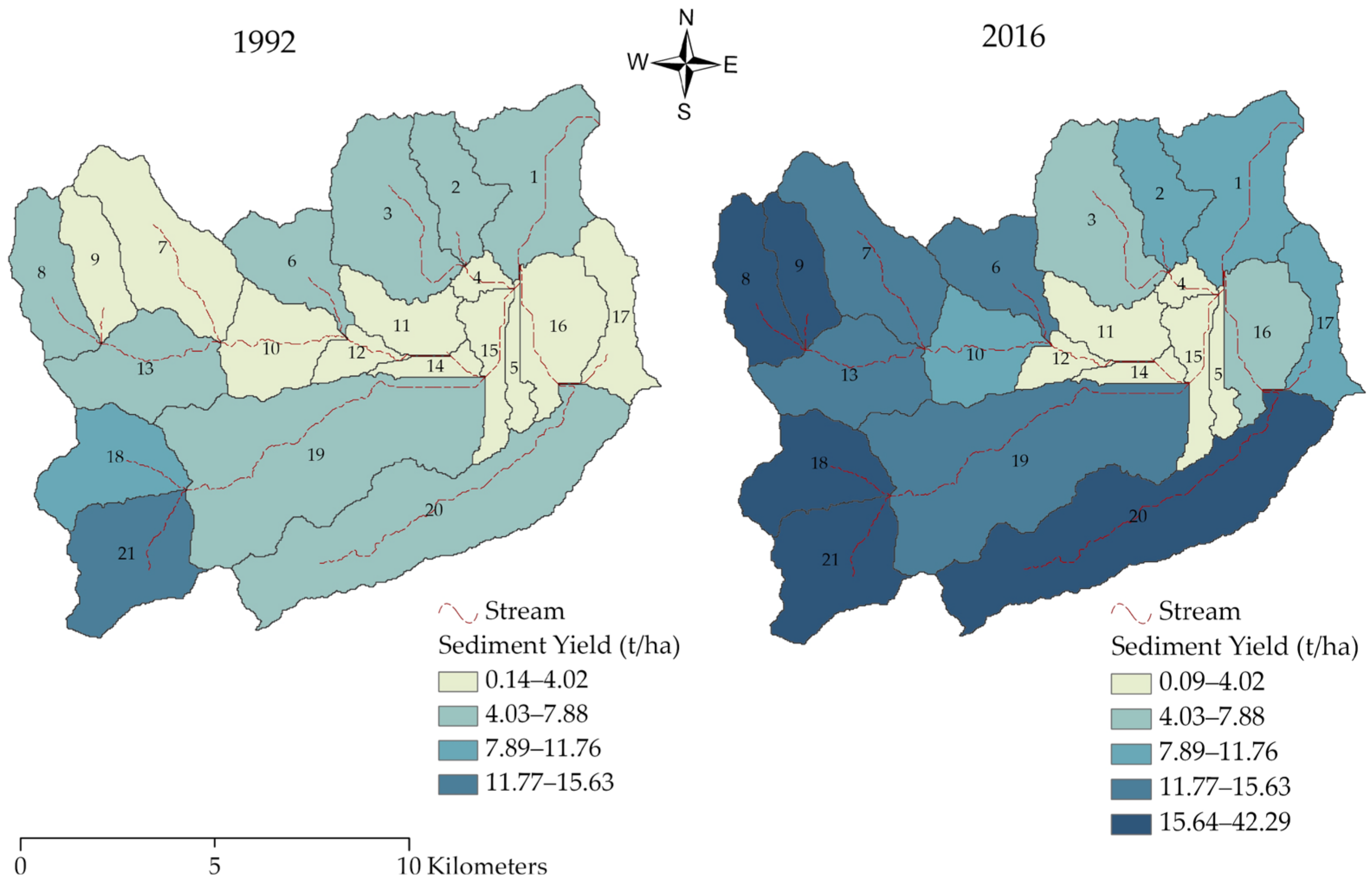
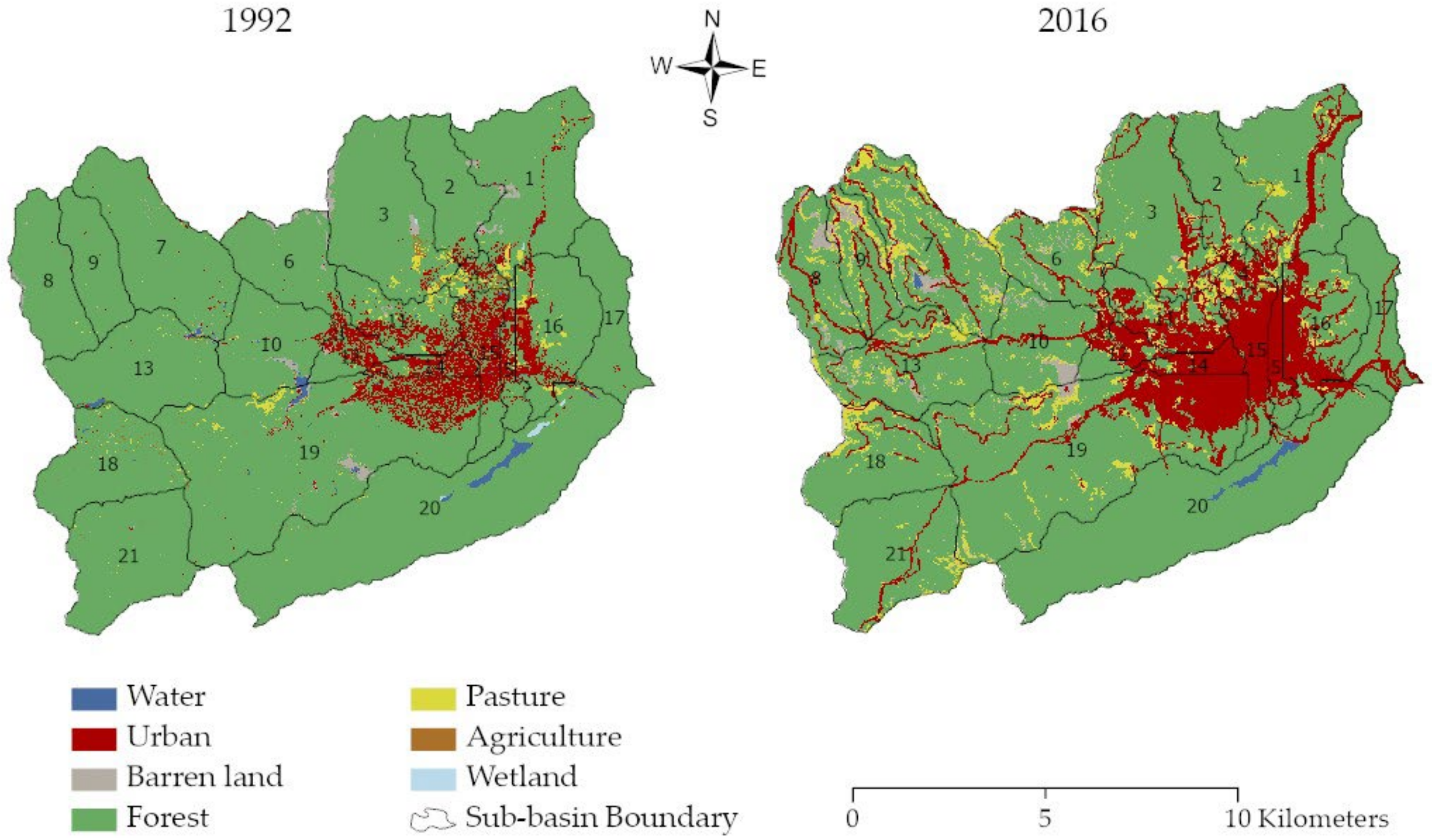
A threshold critical source area of 350 ha (between the suggested range by ArcGIS watershed delineation interface) was used for this study, which divided the watershed into 21 sub-basins (Figure 3a). It was based on the understanding that a smaller threshold generates a denser stream network in the watershed [53]. The LULC maps of 1992 (NLCD) and 2016 (CropScape-Cropland Data) were aggregated into seven LULC types: Water, Urban, Barren, Forest, Pasture, Agriculture, and Wetland. SSURGO, a higher resolution soil map, defined 38 different soil types in the watershed. The slopes were classified into four classes: 0–15%, 15–30%, 30–45% and >45%. We opted out threshold (LULC/Soil/Slope: 0/0/0[%]) in HRU definition, which resulted in the further partition of sub-basins into 1847 HRUs (Figure 3b).

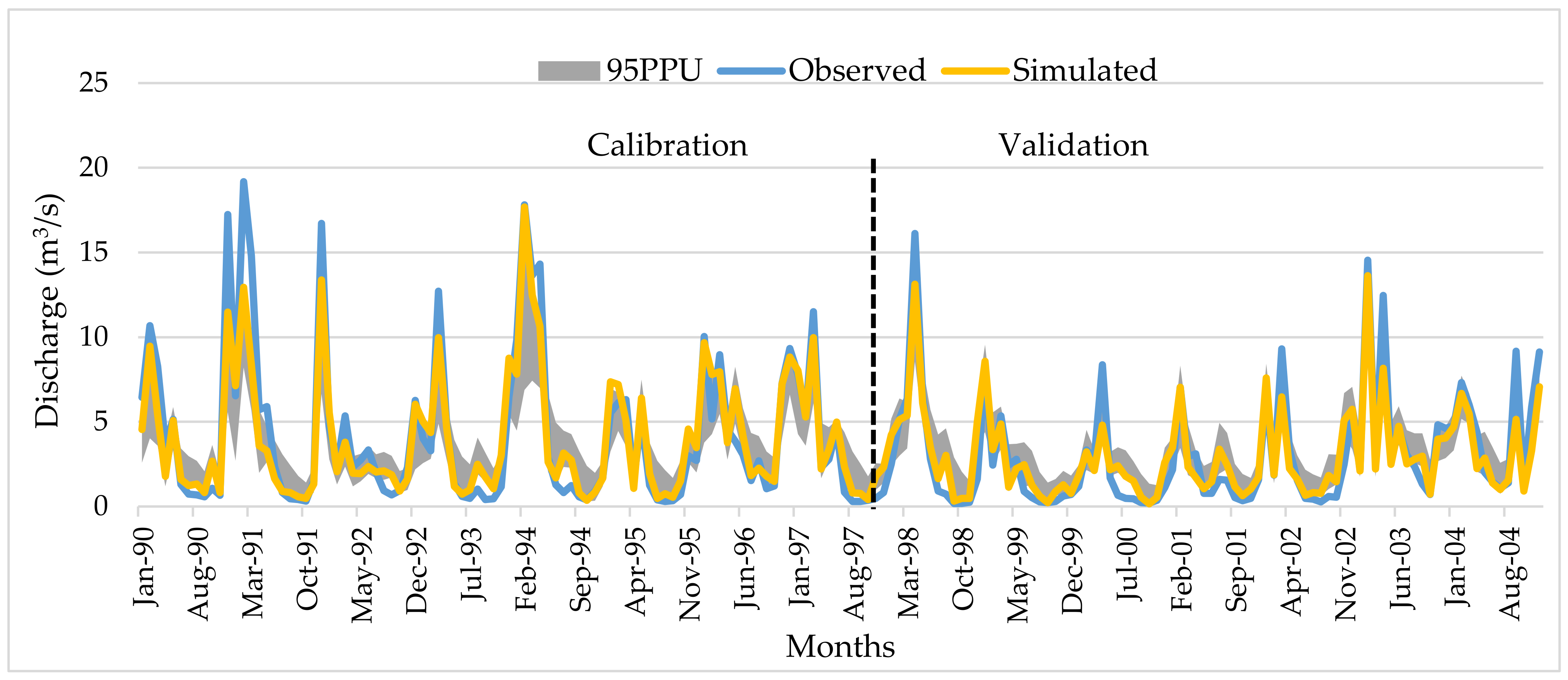
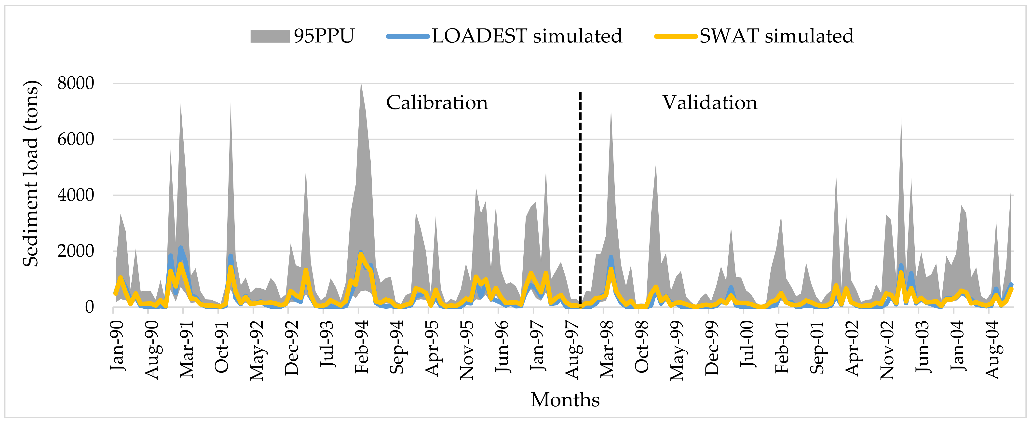
The SWAT model was set up to run for 18 years from 1 January 1987 to 31 December 2004. The period of 1 January 1987, to 31 December 1989, was considered a “warm-up” period. The remaining available years were divided into calibration and validation periods that extended from 1990–1997 and 1998–2004, respectively. After calibration and validation of the SWAT model based on LULC 1992, the model was rerun with the LULC of 2016 with the best parameter values for the 2005–2016 period.

2.5. SWAT-CUP Premium and SWAT Parameter Estimator (SPE) Algorithm

We used SWAT-CUP Premium (SWAT-CUPP), a computer program developed for calibration of the SWAT model (https://www.2w2e.com/home/SwatCupPremium; accessed on 17 February 2021). SWAT-CUPP is an improved version of SWAT-CUP, which allows for behavioral and multi-objective calibration [54].

SWAT-CUPP offers two algorithms, SWAT Parameter Estimator (SPE) and Particle Swarm Optimization (PSO). We used the SPE algorithm (previously Sequential Uncertainty Fitting (SUFI-2)) for model sensitivity analysis, calibration, uncertainty analysis, and validation [5,13]. In SPE, the algorithm maps all uncertainties (parameter, conceptual model, input, etc.) on the parameters (expressed as uniform distributions or ranges) and tries to capture most of the measured data within the 95% prediction uncertainty (95PPU) of the model in an iterative process determined at the 2.5% and 97.5% levels of cumulative distribution of output variables obtained through Latin hypercube sampling [54,55]. Users are provided with several choices of objective function (11 functions including the Nash-Sutcliffe Efficiency coefficient (NSE), the coefficient of determination (R²), and percent bias (PBIAS)). We selected NSE as our objective function in this study because it is recommended to be the best objective function for reflecting the overall fit of a hydrograph [56,57]. NSE is a normalized statistic that determines the relative magnitude of the residual variance compared to the measured data variance [58]. NSE is computed as

$$\mathit{NSE}=1–\frac{{{\displaystyle \sum }}_{i=1}^n{{(Y}_i^{\mathit{obs}}{-Y}_i^{\mathit{sim}})}^2}{{{\displaystyle \sum }}_{i=1}^n{{(Y}_i^{\mathit{obs}}{-Y}_i^{\mathit{mean}})}^2}$$

(6)

where $Y_i^{\mathit{obs}}$ is the ith observation for the constituent being evaluated, $Y_i^{\mathit{sim}}$ is the ith simulated value for the constituent being evaluated, $Y_i^{\mathit{mean}}$ is the mean of observed data for the constituent being evaluated, and n is the total number of observations [59]. The details of the SWAT-CUPP and SPE algorithms can be found in the SWAT-CUPP user manual [54].

2.6. Model Sensitivity Analysis

Sensitivity analysis is the foremost step in the calibration and validation process in SWAT-CUPP, which determines the most sensitive parameters for a given watershed [55]. SPE is embedded with two systems for sensitivity analysis (i.e., one-at-a-time and global). This study utilizes both: one-at-a-time sensitivity analysis to identify the sensitive parameters and global sensitivity analysis to define the rank of the model parameters.

One-at-a-time sensitivity analysis was conducted for each parameter while keeping other parameter values constant [54]. In global sensitivity analysis, a multiple regression system regresses the Latin hypercube-generated parameters against objective function values to determine the sensitivity of the parameters [54]. The sensitivity is calculated according to

$$g=\alpha +{\displaystyle \sum }_{i=1}^m{\beta }_i{b}_i$$

(7)

where g denotes the objective function, b is the parameter, $\alpha$ is the regression constant, $\beta$ corresponds to the technical coefficient attached to the variable b, and m is the number of parameters [60].

In addition, statistical measurements t-stat and p-value were used to identify the sensitive parameters, with larger t-stats and smaller p-values representing greater sensitivity. Based on one-at-a-time sensitivity analysis, Abbaspour et al. [60], and the relevant literature [45,47,61], a total of 30 parameters (see

Table A2. SWAT parameter range and description.

Parameters for Both Variables
Input Parameter	Description	Initial Range
CN2.mgt	SCS runoff curve number	35–98
2. ESCO.hru	Soil evaporation compensation factor	0–1
3. EPCO.hru	Plant uptake compensation factor	0–1
4. HRU_SLP.hru	Average slope steepness	0–0.6
5. SLSUBBSN.hru	Average slope length	10–150
6. OV_N.hru	Manning’s “n” value for overland flow	0.01–4
7. GWQMN.gw	Threshold depth of water in the shallow aquifer required for return flow to occur (mm)	0–5000
8. REVAPMN.gw	Threshold depth of water in the shallow aquifer for “revap” to occur (mm)	0–1000
9. GW_REVAP.gw	Groundwater “revap” coefficient	0.02–0.2
10. ALPHA_BF.gw	Baseflow alpha factor (days)	0–1
11. GW_DELAY.gw	Groundwater delay (days)	0–500
12. RCHRG_DP.gw	Deep aquifer percolation fraction	0–1
13. SOL_K.sol	Saturated hydraulic conductivity	0–2000
14. SOL_BD.sol	Moist bulk density	0.9–2.5
15. SOL_AWC.sol	Available water capacity of the soil layer	0–1
16. CH_N2.rte	Manning’s “n” value for the main channel	−0.01–0.3
17. CH_K2.rte	Effective hydraulic conductivity in main channel alluvium	−0.01–500
18. SURLAG.bsn	Surface runoff lag time	0.025–24
19. SFTMP	Snowfall temperature	−10–10
20. SMTMP	Snow melt base temperature	−10–10
21. SMFMX	Maximum melt rate for snow during year	0–10
22. SMFMN	Minimum melt rate for snow during the year	0–10
23. TIMP	Snow pack temperature lag factor	0–1
Parameters for Sediment Only
Input Parameter	Description	Initial Range
24. SPEXP.bsn	Channel re-entrained exponent parameter	1–1.5
25. SPCON.bsn	Sediment re-entrained linear parameter	0.0001–0.01
26. PRF.bsn	Sediment routing factor in main channels	0–2
27. USLE_P.mgt	Support practice factor	0–1
28. USLE_K.sol	Soil erodability factor	0–0.65
29. CH_COV1.rte	Channel erodability factor	−0.05–0.6
30. CH_COV2.rte	Channel cover factor	−0.001–1

) were selected for global sensitivity analysis. To perform global sensitivity analysis, we ran our first iteration among 23 selected parameters for discharge. Our first iteration was run with 600 simulations. In our analysis, the larger the value of t-stat (in absolute value) and the smaller the p-value (p < 0.05), the more sensitive the parameters were [54]. Once the satisfactory calibration performance was obtained for discharge, sensitivity analysis was carried out for the sediment parameters with a similar approach. The initial parameter ranges were set according to the SWAT manual and available guidelines [23,47,55] (see Table A2).

The results of global sensitivity analysis after the first iteration are listed in

Table 2. List of sensitive parameters (p < 0.05) (ranked in descending order) to discharge and sediment (v = replace, r = relative).

Sensitivity of Parameters to Discharge					Sensitivity of Parameters to Sediment
Parameter Name	t-Stat	p-Value	Calibration Range	Fitted Value	Parameter Name	t-Stat	p-Value	Calibration Range	Fitted Value
v__ALPHA_BF.gw	14.63	0.00	0–0.6	0.45	v__CH_N2.rte	10.914	0.00	−0.01–0.12	0.05
r__CN2.mgt	7.57	0.00	0.1–0.3	0.16	v__GWQMN.gw	−2.74		240–1128	673.75
v__CH_K2.rte	−10.07	0.00	−0.01–50	18.28	r__CN2.mgt	−2.08	0.03	0.06–0.2	0.08
v__GWQMN.gw	−10.91	0.00	0–2565	378.33	v__SPEXP.bsn	2.01	0.04	1.16–1.38	1.37
v__CH_N2.rte	−5.17	0.00	−0.01–0.3	0.03
r__SOL_BD().sol	4.24	0.00	−0.6–0.01	−0.51
v__GW_DELAY.gw	−3.80	0.00	0–52	4.73
v__SFTMP.bsn	−3.93	0.00	−5–5	−4.31
r__SOL_AWC().sol	−3.62	0.00	−0.1–0.02	−0.005
r__SOL_K().sol	2.99	0.01	−0.6–0.2	−0.64
v__GW_REVAP.gw	−2.68	0.01	0.02–0.14	0.04
v__ESCO.hru	2.55	0.01	0.3–0.7	0.53
r__HRU_SLP.hru	2.29	0.02	−0.5–0.4	−0.10
v__SMFMN.bsn	2.17	0.03	0–10	4.78
r__SLSUBBSN.hru	−2.09	0.04	−0.5–0.02	−0.42

. The parameters related to groundwater (ALPHA_BF, GWQMN, GW_DELAY, and GW_REVAP), runoff curve number (CN2), channel routing (CH_K2 and CH_N2), soil (SOL_BD, SOL_AWC, SOL_K, and ESCO), snow (SFTMP and SMFMN), and topography (HRU_SLP and SLSUBBSN) were the most sensitive (p < 0.05) to discharge. Sediment was most sensitive (p < 0.05) to routing parameter (CH_N2), groundwater (GWQMN), runoff curve number (CN2), and channel re-entrained exponent parameter (SPEXP).

2.7. Model Calibration and Uncertainty Analysis

The second step is model calibration, in which parameter value ranges are adjusted to improve the fit between model predictions and real-world observations [47]. SWAT-CUPP allows users to select specific model parameters for auto-calibration within their acceptable ranges (see Table A2) and execute hundreds of SWAT simulations to find the optimal set of parameter values that minimizes the error between model predictions and observed data [54,55]. During calibration of parameters, only sensitive parameters (Table 2) were calibrated based on the results of the sensitivity analysis in SWAT-CUPP.

Calibration is characteristically subjective and, therefore, closely linked to model output uncertainty [24,55]. The term uncertainty analysis refers to the propagation of all model input errors and uncertainties to model outputs. In SWAT-CUPP, two indices referred to as “P-factor” and “R-factor” are used to quantify the fit between simulation results [24,47,55,60]. The P-factor is the fraction of measured data (plus its error) bracketed by the 95PPU band, and the average distance $\overline{d}$ between the upper and the lower 95PPU (or the degree of uncertainty) estimated from

$${\overline{d}}_X=\frac{1}{k}{{\displaystyle \sum }}_{l=1}^k{{(X}_U {–X}_L)}_l$$

(8)

where k is the number of observed data points, $l$ is a counter and $X_L$ (2.5th) and $X_U$ (97.5th) represent the lower and upper boundaries of the 95PPU [54,55,60]. The P-factor varies from 0 to 1, where 1 indicates 100% bracketing of the measured data within model prediction uncertainty (i.e., a perfect model simulation considering the uncertainty). The R-factor is the ratio of the average width of the 95PPU band and the standard deviation of the measured variable. The R-factor is estimated by

$$R-\mathit{factor}=\frac{{\overline{d}}_X}{{\sigma }_X}$$

(9)

where ${\sigma }_X$ is the standard deviation of the measured variable X. The P-factor value of >0.7 (at least 70%) and R-factor value of <1.5 (at most 150%) are desirable and recommended to be adequate [60,62]. However, depending on the project scale and availability of input and calibration data, these requirements can be adaptable [24,60,62]. In general, a larger P-factor can be achieved at the cost of a larger R-factor. A balance between the two must, therefore, always be considered. When appropriate values of R-factor and P-factor are achieved, the parameter ranges are taken as the calibration parameters in the final iteration. However, it is important to understand that there is no single good solution representing model output but rather an envelope of good solutions expressed by the 95PPU, with certain parameter ranges [24].

2.8. Model Validation

After calibration, the model is validated with the calibrated parameter ranges and by comparing predictions to additional observed data, which is not used for calibration. Based on the level of agreement between predictions and the additional observations, the model is validated for further use, or model inputs and parameters are revisited for further calibration [47,56]. Similar to calibration, validation results are also quantified by the P-factor and R-factor.

The initial model obtained from ArcSWAT was divided into two periods, 1990–1997 for calibration and 1998–2004 for validation in SWAT-CUPP. Discharge was calibrated first since it is the primary controlling variable [54]. After running the one-at-a-time sensitivity analysis and following the literature [5,24,45,61], the model was parameterized, and ranges were assigned. The model was run for three iterations (600 simulations each) for calibration. After each iteration, new parameter ranges were suggested, which were used for another round of iteration. Finally, the model was run for another iteration (600 simulations) with the calibrated parameter ranges for validation. A similar procedure was applied for the calibration and validation of sediment.

Parallel processing was utilized to speed up the calibration process. The parallel processing module utilized all eight CPUs where, for each iteration, 600 simulations were divided into eight simultaneous runs of 75 each per CPU. This substantially improved the runtime of the calibration and validation process [54].

2.9. Model Performance Indices

In addition to two indices used for prediction uncertainty analysis, P-factor and R-factor, multiple indices are made available to check the performance of the SWAT model [59]. In this study, the Nash-Sutcliffe efficiency coefficient (NSE), RMSE-observations standard deviation ratio (RSR), percent bias (PBIAS), and the coefficient of determination (R²) were used to evaluate calibration and validation performance of the SWAT model. These are among some of the most widely used indices. NSE indicates how well the observed versus simulated data plot fits within the 1:1 line [59]. NSE ranges between −∞ and 1, with NSE = 1 being the optimal value. RSR is the ratio of RMSE and the standard deviation of observed value, with a lower value being the better model simulation performance [59]. PBIAS, with an optimal value of 0, evaluates the average tendency of the simulated data to be greater or lesser than their observed counterparts [63]. The low values of PBIAS imply accurate model simulation, positive values indicate model underestimation, and negative values indicate model overestimation bias [59]. The proportion of the variance in measured data explained by the model is described by R² [63]. The value of R² ranges from 0 to 1, with higher values indicating less error variance [59,64]. More details on the thresholds for evaluation of model performance can be found in Moriasi et al. [59,65] (see

Table A3. Statistics recommended by Moriasi et al. [59,65] to evaluate the performance of the SWAT model.

	Component	Very Good	Good	Satisfactory	Not Satisfactory
NSE	Discharge	NSE > 80	0.70 < NSE ≤ 0.80	0.50 < NSE ≤ 0.70	NSE ≤ 0.50
	Sediment	NSE > 80	0.70 < NSE ≤ 0.80	0.45 < NSE ≤ 0.70	NSE ≤ 0.45
R2	Discharge	R2 > 85	0.75 < NSE ≤ 0.85	0.60 < NSE ≤ 0.75	R2 ≤ 0.60
	Sediment	R2 > 80	0.65 < NSE ≤0.80	0.40 < NSE ≤ 0.65	R2 ≤ 0.40
PBIAS	Discharge	PBIAS < ±5	±5 < PBIAS < ±10	±10 ≤ PBIAS < ±15	PBIAS ≥ ±15
	Sediment	PBIAS < ±10	±10 < PBIAS < ±15	±10 ≤ PBIAS < ±20	PBIAS ≥ ±20
RSR	Discharge/Sediment	0.00 ≤ RSR ≤ 0.50	0.50 < RSR ≤ 0.60	0.60 < RSR ≤ 0.70	RSR > 0.70

).

3. Results

3.1. Model Calibration, Uncertainty Analysis, and Validation

After performing three iterations (600 simulations in each) with modifications to the parameters, the model was observed to have a good fit between the observed and simulated discharge and between the LOADEST-simulated and SWAT-simulated sediment. The statistical results of the model performance for discharge and sediment during both calibration and validation periods are summarized in

Table 3. Statistical results of calibration and validation.

Discharge	P-Factor	R-Factor	NSE	RSR	R2	PBIAS
Calibration (1990–1997)	0.58	0.58	0.87	0.36	0.89	2.8
Validation (1998–2004)	0.62	0.69	0.84	0.40	0.86	−0.4
Sediment	P-Factor	R-Factor	NSE	RSR	R2	PBIAS
Calibration (1990–1997)	0.55	3.15	0.86	0.38	0.88	−18.8
Validation (1998–2004)	0.46	4.19	0.81	0.44	0.84	−15.9

. The calibration and validation of discharge and sediment are illustrated as a 95PPU graph in Figure 4 and Figure 5, respectively.

Graphical results during both calibration and validation (Figure 4) indicated adequate performance over the range of discharge. The calibrated model achieved both the P-factor and R-factor of 0.58. This explains that 58% of the measured discharge was bracketed by 95PPU within model prediction uncertainty. The 95PPU bracketed about 62% of the measurement in the validation period, which is higher than the calibration period. Similarly, the R-factor had the desired values of 0.58 and 0.69 (R-factor < 1.5). Overall, the NSE values (0.87 and 0.84) indicate a good match between measured and simulated monthly discharge for the calibration and validation period. The RSR values were 0.36 and 0.40 during the calibration and validation period. These values indicated a very good model performance for residual discharge variation. The R² (0.89 and 0.86) showed a strong linear correlation between measured and simulated monthly discharge. PBIAS values were 2.8 and –0.4 for calibration and validation, respectively. These values were also within the “very good” range (PBIAS < ±5) according to the guidelines [59,65].

The 95PPU bracketed about 55% of the observations in the case of sediment load calibration (Figure 5). Additionally, NSE (0.86), RSR (0.38), and R² (0.88) were excellent statistics. However, the PBIAS value (−18.8) could only be of a satisfactory level for the calibration period. In comparison to a calibration period, the validation period (Figure 5) reached a lower P-factor (0.46). However, considerably impressive results were recorded for NSE (0.81), RSR (0.44), and R² (0.84). Similar to calibration, the validation period also achieved a satisfactory result with PBIAS (−15.9). In sediment load calibration and validation, the model achieved R-factor values of 3.15 and 4.19, respectively. Overall, it can be evaluated as a good model based on the criteria by Moriasi et al. [59,65].

3.2. Impact of LULC Change on the Water Balance Components in Yellow Creek Watershed

The annual summaries of water balance components between 1992 and 2016 are listed in

Table 4. Impact of LULC change on the water balance components in the Yellow Creek Watershed.

Year	1992	2016	% Change
Precipitation (mm)	1304.84	1268.75	−2.76
Surface Runoff (mm)	125.66	209.66	+66.85
Lateral Flow (mm)	207.39	113.44	−45.30
Groundwater (mm)	105.49	81.83	−22.43
Percolation (mm)	209.41	177.1	−15.43
Potential Evapotranspiration (mm)	900.6	1086.87	+20.68
Water Yield (mm)	462.37	424.19	−8.26
Sediment Yield (t/ha)	5.34	14.66	+174.53

. Results show that total yearly precipitation, lateral flow, and groundwater experienced a decrease of 2.76%, 45.3%, and 22.43%, respectively, whereas surface runoff increased by 66.85% from 1992 to 2016. Loss of water due to percolation accounted for about a 15.43% decrease from 1992 to 2016. There was a slight increase in evapotranspiration (0.32%), while the potential evapotranspiration witnessed a 20.68% increment from 1992 to 2016. Overall, the total annual water yield decreased from 462.37 mm in 1992 to 424.19 mm in 2016. Between 1992 and 2016, sediment yield increased from 5.34 t/ha to 14.66 t/ha.

Figure 6 and Figure 7 illustrate the distribution of the annual water balance components in 1992 and 2016. Total annual precipitation varied from 1096.60 mm to 1534.56 mm at the sub-basin scale in 1992. Sub-basins 6, 7, 8, 9, and 13 received the highest precipitation, whereas sub-basins 1, 2, and 12 recorded the lowest. The overall range of precipitation declined in 2016 (1176.73–1344.41 mm), with the highest amount of precipitation at sub-basins located in the northwest and southwest regions of the watershed. Potential evapotranspiration ranged from 861.17 mm to 943.51 mm in 1992, where sub-basins 4, 5, and 14 had the highest and sub-basins 8, 9, and 18 had the lowest amounts. Total annual potential evapotranspiration increased in 2016, which varied from 1062.41 mm to 1102 mm.

Figure 7 depicts sub-basins in the northwest and southwest region that witnessed the highest amount of potential evapotranspiration in 2016, whereas it was lowest in sub-basins in the central and eastern side of the watershed. Percolation ranged from 132.76 mm to 150.76 mm and 114.83 mm to 139.81 mm in 1992 and 2016, respectively, with sub-basins located on the northeast side of the watershed witnessing the highest amount. In 1992, the amount of lateral flow ranged from 3.32 mm to 322.29 mm, with a similar spatial distribution to percolation. In 2016, there was a decline in lateral flow, with the lowest range of 2.09–33.01 mm in sub-basins located in the central region of the watershed to the highest range of 269.44–322.29 mm in sub-basins situated in the northeast side of the watershed. Surface runoff varied from 42.41 mm to 82.22 mm in 1992, whereas it increased in 2016 with the lowest value of 118.64 mm to the highest of 353.96 mm. Finally, the total annual values of groundwater ranged from 44.13 mm to 196.75 mm in 1992, which declined in 2016 to the range of 30.07–133.97 mm.

3.3. Sediment Yield and LULC Change in Yellow Creek Watershed

The spatial distribution of sediment yield in 1992 and 2016 within the Yellow Creek Watershed is illustrated in Figure 8. In 1992, the total sediment yield ranged from 0.14 t/ha to 15.63 t/ha, where sub-basin 21 recorded the highest sediment yield, followed by sub-basin 18. In 2016, the sediment yield increased significantly, ranging from 0.09 t/ha to 42.29 t/ha. Sub-basins 8, 9, 18, 20, and 21 yielded the highest sediment (>15.64 t/ha). Except for sub-basins 3, 4, 5, 11, 12, 14, and 15, all sub-basins experienced an increase in sediment yield.

As illustrated in

Table 5. LULC change from 1992 to 2016 in Yellow Creek Watershed.

Land Cover Type	1992		2016		Change (ha)	% Change of 1992	% Change of Total Area
	Area (ha)	%	Area (ha)	%
Water	0.80	0.51	0.52	0.33	−0.28	−0.18	−0.01
Urban	9.35	5.95	24.17	15.37	14.82	9.43	5.99
Barren Land	1.56	0.99	3.14	2.0	1.58	1.01	0.64
Forest	142.84	90.88	119.67	76.14	−23.17	−14.74	−9.37
Pasture	1.72	1.09	9.60	6.11	7.88	5.02	3.19
Agriculture	0.78	0.50	0.08	0.05	−0.70	−0.45	−0.28
Wetland	0.13	0.08	0.002	0.001	−0.12	−0.079	−0.05
Total	157.18	100	157.18	100

, a comparison between 1992 and 2016 reveals that all LULC classes have undergone some changes. In the last 25 years, the changes in each LULC ranged from 0.05% to 9.37% of the total watershed area. The highest percentage of change occurred in forested areas, by a total of 14.74%. The change can be attributed to the conversion of forest area into urban development, pasture, and barren land, which increased by 9.43%, 5.02%, and 1.01%, respectively. Similarly, agriculture and water also declined by 0.45% and 0.18%, respectively. The wetland area declined by 0.079%, which only covered 0.02 ha in 2016.

Furthermore, the spatial distribution of LULC classes in 1992 and 2016 is illustrated in Figure 9. The northwestern region of the watershed experienced the most intensive changes in forest cover. Sub-basins heavily forested in 1992 converted into barren lands, pastures, and urban developments in 2016. Overall, the change in forest cover is more or less found to be distributed in all sub-basins. Conversion of LULC in the form of barren land in 2016 is primarily attributed to the development of coal-mining lands, which can be seen in sub-basins 7, 8, 9, and 10 (Figure 9). As evident in Figure 8, these sub-basins contributed the highest sediment yield in 2016. Moreover, the increase in sediment yield seems to be mainly associated with sediment transport from barren lands (mining fields), urban development activities, and pasturelands [9,66,67,68]. This implies that the sediment yield increased due to the direct and indirect consequences of LULC changes in the watershed.

Figure 9 also shows barren land areas in 1992 (Sub-basins 1, 3, & 19) converted into other classes. This may be the result of various post-mining reclamation practices that have been implemented in the watershed [69,70]. Additionally, some forest-dominated regions (sub-basin 20) witnessed an increase in sediment in 2016. This might be attributed to comparatively steeper slopes in some regions. As seen in this study, sub-basins with the greatest sediment yield had a slope of more than 30% (Figure 2 and Figure 8). Furthermore, studies have demonstrated a significant correlation between sediment yield and slope gradient [71,72].

4. Discussion

The resulting statistics of our study were acceptable based on the guidelines [59,65], and were similar to values found in other studies conducted in the United States [5,13,45,73,74,75,76,77] and around the world [4,45,46,47,48,49,50]. Spruill et al. [45] reported the SWAT model as an effective model for simulating monthly runoff in a small watershed in central Kentucky, with NSE values of 0.89 (calibration) and 0.58 (validation). Coffey et al. [78] stated similar results for the same watershed. Shrestha et al. [5] used SWAT to study industrial wood pellet impact on streamflow in Georgia. In the latter study, predicted values compared well with observed values, with NSE and R² values above 0.75, and predicted streamflow 3.57–7.28% lower than the observed streamflow. In their study in North Carolina, Ayivi and Jha [79] reported a good agreement for discharge, with both NSE and R² values greater than 0.70. In another study conducted by Tadesse et al. [73] in a watershed located in Tennessee and Alabama, the model adequately simulated sediment with R² and NSE values of 0.71 and 0.70, respectively. Compared to these studies, our model achieved adequate statistics, which indicates a much better correlation with NSE values higher than 0.80 for both calibration and validation periods.

The results from this study imply that LULC modification might have a significant impact on the annual water balance in the watershed. The decline in percolation, lateral flow, and groundwater might be mainly due to changes in LULC and altered soil properties due to coal-mining activities in the watershed. Similarly, increased runoff indicated the lower infiltration capacity of the surface. Evidence from previous studies also suggests the historical LULC change impact in basin-scale water balance, such as with the Raccoon River Watershed in Iowa [13], the Little River Watershed in Tennessee [3], the Kentucky River Basin [46], and the Reedy Fork-Buffalo Creek Watershed in North Carolina [79].

Our findings are consistent with previous studies that suggest increasing sediment yields, water quality degradation, and increasing flood events pertaining to LULC changes [9,73] caused by the clear-cutting of forests. The increase in sediment yield indicates an impact of LULC changes in the Yellow Creek Watershed. As seen, sub-basins dominant with barren lands and pastures contributed most in sediment yield. It may be due to mining activities and emerging pastures in the reclaimed mine lands [9,69,70]. According to the report prepared by the Appalachian Regional Commission, coal production has fallen by more than 45% in Appalachia between 2005 and 2015 due to the depletion of high-grade coal seams [80]. However, a recent study showed that the cumulative mining area is still increasing in central Appalachia, though at a significantly lower growth rate [9,81]. The continuous growth of cumulative mines indicates that mining might still be a key driving factor in the LULC transformation in some Appalachian Mountains areas [9,69,70].

Several studies show higher peak and total storm runoff from mined lands compared to forested lands in the Appalachian region [82,83]. These results suggest that surface mining may increase the risks of more flooding hazards and recommend more studies for quantification and evaluation of the effects of mined land conversions in the region. Knowledge of the extent of mining is critical to managing or mitigating the potential impacts of surface mining on sedimentation.

SWAT is an effective and widely accepted tool in predicting the impact of LULC changes [23,47]; however, success of SWAT depends on the quality of input data, such as the resolution of the DEM, LULC data, and soil [23,84]. In our study, given the availability of data, we were limited to moderate resolution data (30 m × 30 m) such as NLCD LULC data. Precipitation is a crucial factor affecting runoff events and sediment export. In SWAT, precipitation is simulated in each sub-basin according to the nearest gauge to the sub-basin centroid [85]. Having a sufficient number of gauges in a watershed is, therefore, incredibly beneficial for hydrological simulations in SWAT. However, our analysis was restricted by the absence of ground observation data, and substitute methods such as PRISM climate data were utilized.

5. Conclusions

This study was successful in simulating sediment yield and quantifying the impact of LULC change on the hydrology of the watershed. The results showed a very good agreement between observed and predicted discharge and sediment at the outlet. The results showed that the Yellow Creek Watershed experienced LULC changes over 25 years between 1992 and 2016. It consisted primarily of a decrease in forest cover which mostly converted into coal-mine lands, urban development, and growth in pastureland. Similarly, the comparison of the distribution of water balance components, sediment yield, and LULC changes in the watershed implied that LULC changes, specifically ongoing surface mining activities, increasing pastureland, and urban development, have contributed to augmenting the sediment yield in the watershed.

This study contributes to studying land management practices in watersheds impaired by coal-mine operations. Addressing impacts of LULC change issues strategically and timely is essential for the effective management of coal-mine lands and water resources. Identifying critical areas and selecting best management practices (BMPs) in watershed scale are necessary for reducing sedimentation. The BMPs in watershed scale, for example, should focus on approaches for reducing the environmental footprints of mining by implementing reclamation practices that are feasible in the watershed.

Despite model and data limitations, this study fills the gap that exists in modeling LULC impacts on water and land management in the coal-mine lands of the Appalachian region in Kentucky. The findings presented provide a plethora of information on LULC changes and their impact on hydrology. The maps and tables produced in this study provide essential spatial information on the sub-basin scale to researchers in identifying and implementing appropriate land management practices.

There is a dearth of systematic research and data to quantify the effects of coal-mine lands on increased surface runoff and sediment yield. This research is a case study modeling impacts of LULC on runoff and sediment yield. We recommend continuing similar studies in the other watersheds to discern the role of change in LULC on runoff and sediment yield using high-resolution land cover data and integrating such data with human populations and infrastructure changes such as access roads to coal mine areas. Future studies should include local rainfall characteristics and evapotranspiration data. Rainfall patterns and their impacts on coal-field areas will be important to study in this region.

In future studies, this approach can further be utilized in other similar watersheds to explore the impacts of surface-mining activities on the hydrological properties and to evaluate the effectiveness of best management practices (BMPs) in managing sediment yields for environmental stewardship at the watershed level. We will expand this research to include other watersheds from the Appalachian region to explore the impacts of land-use change on water discharge, as well as the effects of current agricultural and forestry-related BMPs in sediment control and management.

References

1. Lambin, E.F.; Turner, B.L.; Geist, H.J.; Agbola, S.B.; Angelsen, A.; Bruce, J.W.; Coomes, O.T.; Dirzo, R.; Fischer, G.; Folke, C.; et al. The Causes of Land-Use and Land-Cover Change: Moving beyond the Myths. Glob. Environ. Chang. 2001, 11, 261–269. [Google Scholar] [CrossRef]
2. Turner, B.L. Local Faces, Global Flows: The Role of Land Use and Land Cover in Global Environmental Change. Land Degrad. Dev. 1994, 5, 71–78. [Google Scholar] [CrossRef]
3. Zhu, C.; Li, Y. Long-Term Hydrological Impacts of Land Use/Land Cover Change From 1984 to 2010 in the Little River Watershed, Tennessee. Int. Soil Water Conserv. Res. 2014, 2, 11–21. [Google Scholar] [CrossRef] [Green Version]
4. Pokhrel, B.K. Impact of Land Use Change on Flow and Sediment Yields in the Khokana Outlet of the Bagmati River, Kathmandu, Nepal. Hydrology 2018, 5, 22. [Google Scholar] [CrossRef] [Green Version]
5. Shrestha, S.; Dwivedi, P.; McKay, S.K.; Radcliffe, D. Assessing the Potential Impact of Rising Production of Industrial Wood Pellets on Streamflow in the Presence of Projected Changes in Land Use and Climate: A Case Study from the Oconee River Basin in Georgia, United States. Water 2019, 11, 142. [Google Scholar] [CrossRef] [Green Version]
6. Shrestha, S.; Rahimzadeh-Bajgiran, P.; De Urioste-Stone, S. Probing Recent Environmental Changes and Resident Perceptions in Upper Himalaya, Nepal. Remote Sens. Appl. Soc. Environ. 2020, 18, 100315. [Google Scholar] [CrossRef]
7. Deng, X.; Zhao, C.; Yan, H. Systematic Modeling of Impacts of Land Use and Land Cover Changes on Regional Climate: A Review. Adv. Meteorol. 2013, 2013, e317678. [Google Scholar] [CrossRef]
8. Pielke, R.A.; Pitman, A.; Niyogi, D.; Mahmood, R.; McAlpine, C.; Hossain, F.; Goldewijk, K.K.; Nair, U.; Betts, R.; Fall, S.; et al. Land Use/Land Cover Changes and Climate: Modeling Analysis and Observational Evidence. WIREs Clim. Chang. 2011, 2, 828–850. [Google Scholar] [CrossRef]
9. Gurung, K.; Yang, J.; Fang, L. Assessing Ecosystem Services from the Forestry-Based Reclamation of Surface Mined Areas in the North Fork of the Kentucky River Watershed. Forests 2018, 9, 652. [Google Scholar] [CrossRef] [Green Version]
10. Sharma, R.; Rimal, B.; Baral, H.; Nehren, U.; Paudyal, K.; Sharma, S.; Rijal, S.; Ranpal, S.; Acharya, R.P.; Alenazy, A.A.; et al. Impact of Land Cover Change on Ecosystem Services in a Tropical Forested Landscape. Resources 2019, 8, 18. [Google Scholar] [CrossRef] [Green Version]
11. Lone, S.A.; Mayer, I.A. Geo-Spatial Analysis of Land Use/Land Cover Change and Its Impact on the Food Security in District Anantnag of Kashmir Valley. GeoJournal 2019, 84, 785–794. [Google Scholar] [CrossRef]
12. Wolde, Z.; Wei, W.; Likessa, D.; Omari, R.; Ketema, H. Understanding the Impact of Land Use and Land Cover Change on Water–Energy–Food Nexus in the Gidabo Watershed, East African Rift Valley. Nat. Resour. Res. 2021, 30, 2687–2702. [Google Scholar] [CrossRef]
13. Schilling, K.E.; Jha, M.K.; Zhang, Y.-K.; Gassman, P.W.; Wolter, C.F. Impact of Land Use and Land Cover Change on the Water Balance of a Large Agricultural Watershed: Historical Effects and Future Directions. Water Resour. Res. 2008, 44. [Google Scholar] [CrossRef]
14. Wang, Q.; Liu, R.; Men, C.; Guo, L.; Miao, Y. Effects of Dynamic Land Use Inputs on Improvement of SWAT Model Performance and Uncertainty Analysis of Outputs. J. Hydrol. 2018, 563, 874–886. [Google Scholar] [CrossRef]
15. Evans, D.M.; Zipper, C.E.; Hester, E.T.; Schoenholtz, S.H. Hydrologic Effects of Surface Coal Mining in Appalachia (U.S.). JAWRA J. Am. Water Resour. Assoc. 2015, 51, 1436–1452. [Google Scholar] [CrossRef]
16. Poudyal, N.C.; Gyawali, B.R.; Simon, M. Local Residents’ Views of Surface Mining: Perceived Impacts, Subjective Well-Being, and Support for Regulations in Southern Appalachia. J. Clean. Prod. 2019, 217, 530–540. [Google Scholar] [CrossRef]
17. Townsend, P.A.; Helmers, D.P.; Kingdon, C.C.; McNeil, B.E.; de Beurs, K.M.; Eshleman, K.N. Changes in the Extent of Surface Mining and Reclamation in the Central Appalachians Detected Using a 1976–2006 Landsat Time Series. Remote Sens. Environ. 2009, 113, 62–72. [Google Scholar] [CrossRef]
18. U.S. Congress. Surface Mining Control and Reclamation Act of 1977; Public Law 95-87, 30; U.S. Government Printing Office: Washington, DC, USA, 1977.
19. Liang, J.; Wu, K.; Li, Y.; Wei, Z.; Zhuo, P.; Yan, Q.; Luo, X. Impacts of Large-Scale Rare Earth Mining on Surface Runoff, Groundwater, and Evapotranspiration: A Case Study Using SWAT for the Taojiang River Basin in Southern China. Mine Water Environ. 2019, 38, 268–280. [Google Scholar] [CrossRef]
20. Pechlivanidis, I.G.; Jackson, B.M.; Mcintyre, N.R.; Wheater, H.S. Catchment Scale Hydrological Modelling: A Review of Model Types, Calibration Approaches and Uncertainty Analysis Methods in the Context of Recent Developments in Technology and Applications. Glob. Nest J. 2011, 13, 193–214. [Google Scholar] [CrossRef]
21. Teshager, A.D.; Gassman, P.W.; Secchi, S.; Schoof, J.T.; Misgna, G. Modeling Agricultural Watersheds with the Soil and Water Assessment Tool (SWAT): Calibration and Validation with a Novel Procedure for Spatially Explicit HRUs. Environ. Manag. 2016, 57, 894–911. [Google Scholar] [CrossRef] [Green Version]
22. Arnold, J.G.; Srinivasan, R.; Muttiah, R.S.; Williams, J.R. Large Area Hydrologic Modeling and Assessment Part I: Model Development1. J. Am. Water Resour. Assoc. 1998, 34, 73–89. [Google Scholar] [CrossRef]
23. Neitsch, S.L.; Arnold, J.G.; Kiniry, J.R.; Williams, J.R. Soil and Water Assessment Tool Theoretical Documentation Version 2009; Texas Water Resources Institute: College Station, TX, USA, 2009. [Google Scholar]
24. Abbaspour, K.C.; Rouholahnejad, E.; Vaghefi, S.; Srinivasan, R.; Yang, H.; Kløve, B. A Continental-Scale Hydrology and Water Quality Model for Europe: Calibration and Uncertainty of a High-Resolution Large-Scale SWAT Model. J. Hydrol. 2015, 524, 733–752. [Google Scholar] [CrossRef] [Green Version]
25. Tian, Y.Q.; Wang, D.; Chen, R.F.; Huang, W. Using Modeled Runoff to Study DOC Dynamics in Stream and River Flow: A Case Study of an Urban Watershed Southeast of Boston, Massachusetts. Ecol. Eng. 2012, 42, 212–222. [Google Scholar] [CrossRef]
26. Gao, F.; Feng, G.; Ouyang, Y.; Jenkins, J.; Liu, C. Simulating Potential Weekly Stream and Pond Water Available for Irrigation in the Big Sunflower River Watershed of Mississippi Delta. Water 2019, 11, 1271. [Google Scholar] [CrossRef] [Green Version]
27. Kharel, G.; Kirilenko, A. Comparing CMIP-3 and CMIP-5 Climate Projections on Flooding Estimation of Devils Lake of North Dakota, USA. PeerJ 2018, 6, e4711. [Google Scholar] [CrossRef]
28. Wang, R.; Kalin, L. Combined and Synergistic Effects of Climate Change and Urbanization on Water Quality in the Wolf Bay Watershed, Southern Alabama. J. Environ. Sci. 2018, 64, 107–121. [Google Scholar] [CrossRef] [PubMed]
29. Jeong, J.; Kannan, N.; Arnold, J.G. Effects of Urbanization and Climate Change on Stream Health in North-Central Texas. J. Environ. Qual. 2014, 43, 100–109. [Google Scholar] [CrossRef] [PubMed]
30. Heo, J.; Yu, J.; Giardino, R.; Cho, H. Water Resources Response to Climate and Land-Cover Changes in a Semi-Arid Watershed, New Mexico, USA. Terr. Atmos. Ocean. Sci. 2015, 26, 463–474. [Google Scholar] [CrossRef] [Green Version]
31. Wang, R.; Kalin, L.; Kuang, W.; Tian, H. Individual and Combined Effects of Land Use/Cover and Climate Change on Wolf Bay Watershed Streamflow in Southern Alabama. Hydrol. Process. 2014, 28, 5530–5546. [Google Scholar] [CrossRef]
32. Mueller-Warrant, G.W.; Phillips, C.L.; Trippe, K.M. Use of SWAT to Model Impact of Climate Change on Sediment Yield and Agricultural Productivity in Western Oregon, USA. Open J. Mod. Hydrol. 2019, 9, 54–88. [Google Scholar] [CrossRef] [Green Version]
33. Jha, M.K.; Wolter, C.F.; Schilling, K.E.; Gassman, P.W. Assessment of Total Maximum Daily Load Implementation Strategies for Nitrate Impairment of the Raccoon River, Iowa. J. Environ. Qual. 2010, 39, 1317–1327. [Google Scholar] [CrossRef]
34. Mitchell, N.; Kumarasamy, K.; Cho, S.J.; Belmont, P.; Dalzell, B.; Gran, K. Reducing High Flows and Sediment Loading through Increased Water Storage in an Agricultural Watershed of the Upper Midwest, USA. Water 2018, 10, 1053. [Google Scholar] [CrossRef] [Green Version]
35. Pokhrel, B.K.; Paudel, K.P. Assessing the Efficiency of Alternative Best Management Practices to Reduce Nonpoint Source Pollution in a Rural Watershed Located in Louisiana, USA. Water 2019, 11, 1714. [Google Scholar] [CrossRef] [Green Version]
36. Merriman, K.R.; Russell, A.M.; Rachol, C.M.; Daggupati, P.; Srinivasan, R.; Hayhurst, B.A.; Stuntebeck, T.D. Calibration of a Field-Scale Soil and Water Assessment Tool (SWAT) Model with Field Placement of Best Management Practices in Alger Creek, Michigan. Sustainability 2018, 10, 851. [Google Scholar] [CrossRef] [Green Version]
37. Santhi, C.; Srinivasan, R.; Arnold, J.G.; Williams, J.R. A Modeling Approach to Evaluate the Impacts of Water Quality Management Plans Implemented in a Watershed in Texas. Environ. Model. Softw. 2006, 21, 1141–1157. [Google Scholar] [CrossRef]
38. Cibin, R.; Trybula, E.; Chaubey, I.; Brouder, S.M.; Volenec, J.J. Watershed-Scale Impacts of Bioenergy Crops on Hydrology and Water Quality Using Improved SWAT Model. GCB Bioenergy 2016, 8, 837–848. [Google Scholar] [CrossRef]
39. Cho, K.H.; Pachepsky, Y.A.; Kim, J.H.; Kim, J.-W.; Park, M.-H. The Modified SWAT Model for Predicting Fecal Coliforms in the Wachusett Reservoir Watershed, USA. Water Res. 2012, 46, 4750–4760. [Google Scholar] [CrossRef] [PubMed]
40. Zeiger, S.J.; Hubbart, J.A. A SWAT Model Validation of Nested-Scale Contemporaneous Stream Flow, Suspended Sediment and Nutrients from a Multiple-Land-Use Watershed of the Central USA. Sci. Total Environ. 2016, 572, 232–243. [Google Scholar] [CrossRef]
41. Hallouz, F.; Meddi, M.; Mahé, G.; Alirahmani, S.; Keddar, A. Modeling of Discharge and Sediment Transport through the SWAT Model in the Basin of Harraza (Northwest of Algeria). Water Sci. 2018, 32, 79–88. [Google Scholar] [CrossRef] [Green Version]
42. Ang, R.; Oeurng, C. Simulating Streamflow in an Ungauged Catchment of Tonlesap Lake Basin in Cambodia Using Soil and Water Assessment Tool (SWAT) Model. Water Sci. 2018, 32, 89–101. [Google Scholar] [CrossRef] [Green Version]
43. Gautam, S.; Dahal, V.; Bhattarai, R. Impacts of Dem Source, Resolution and Area Threshold Values on SWAT Generated Stream Network and Streamflow in Two Distinct Nepalese Catchments. Environ. Process. 2019, 6, 597–617. [Google Scholar] [CrossRef]
44. Munoth, P.; Goyal, R. Impacts of Land Use Land Cover Change on Runoff and Sediment Yield of Upper Tapi River Sub-Basin, India. Int. J. River Basin Manag. 2020, 18, 177–189. [Google Scholar] [CrossRef]
45. Spruill, C.; Workman, S.; Taraba, J. Simulation of Daily and Monthly Stream Discharge from Small Watersheds Using the SWAT Model. Trans. ASAE 2000, 43, 1431–1439. [Google Scholar] [CrossRef]
46. Chattopadhyay, S.; Edwards, D.R.; Yu, Y.; Hamidisepehr, A. An Assessment of Climate Change Impacts on Future Water Availability and Droughts in the Kentucky River Basin. Environ. Process. 2017, 4, 477–507. [Google Scholar] [CrossRef]
47. Arnold, J.G.; Moriasi, D.N.; Gassman, P.W.; Abbaspour, K.C.; White, M.J.; Srinivasan, R.; Santhi, C.; Harmel, R.D.; van Griensven, A.; van Liew, M.W.; et al. SWAT: Model Use, Calibration, and Validation. Trans. ASABE 2012, 55, 1491–1508. [Google Scholar] [CrossRef]
48. USDA. Soil Conservation Service, National Engineering Handbook; Section 4: Hydrology; USDA: Washington, DC, USA, 1972.
49. Monteith, J.L. Evaporation and Environment. Symp. Soc. Exp. Biol. 1965, 19, 205–234. [Google Scholar]
50. Ritchie, J.T. Model for Predicting Evaporation from a Row Crop with Incomplete Cover. Water Resour. Res. 1972, 8, 1204–1213. [Google Scholar] [CrossRef] [Green Version]
51. Williams, J.R. Spnm, a Model for Predicting Sediment, Phosphorus, and Nitrogen Yields from Agricultural Basins. J. Am. Water Resour. Assoc. 1980, 16, 843–848. [Google Scholar] [CrossRef]
52. Runkel, R.L.; Crawford, C.G.; Cohn, T.A. Load Estimator (LOADEST): A FORTRAN Program for Estimating Constituent Loads in Streams and Rivers; Techniques and Methods; USGS Numbered Series 4-A5; U.S. Geological Survey: Reston, VA, USA, 2004; Volume 4. [CrossRef] [Green Version]
53. Luo, Y.; Su, B.; Yuan, J.; Li, H.; Zhang, Q. GIS Techniques for Watershed Delineation of SWAT Model in Plain Polders. Proc. Environ. Sci. 2011, 10, 2050–2057. [Google Scholar] [CrossRef] [Green Version]
54. Abbaspour, K.C. SWAT-CUP Premium 2020: SWAT Calibration and Uncertainty Programs (Premium Version): A User Manual; Eawag—Swiss Federal Institute of Aquatic Science and Technology: Dübendorf, Switzerland, 2020. [Google Scholar]
55. Abbaspour, K.C.; Vaghefi, S.A.; Srinivasan, R. A Guideline for Successful Calibration and Uncertainty Analysis for Soil and Water Assessment: A Review of Papers from the 2016 International SWAT Conference. Water 2018, 10, 6. [Google Scholar] [CrossRef] [Green Version]
56. Servat, E.; Dezetter, A. Selection of Calibration Objective Fonctions in the Context of Rainfall-Ronoff Modelling in a Sudanese Savannah Area. Hydrol. Sci. J. 1991, 36, 307–330. [Google Scholar] [CrossRef]
57. Null, N. Criteria for Evaluation of Watershed Models. J. Irrig. Drain. Eng. 1993, 119, 429–442. [Google Scholar] [CrossRef]
58. Nash, J.E.; Sutcliffe, J.V. River Flow Forecasting through Conceptual Models Part I—A Discussion of Principles. J. Hydrol. 1970, 10, 282–290. [Google Scholar] [CrossRef]
59. Moriasi, D.N.; Arnold, J.G.; Van Liew, M.W.; Bingner, R.L.; Harmel, R.D.; Veith, T.L. Model Evaluation Guidelines for Systematic Quantification of Accuracy in Watershed Simulations. Trans. ASABE 2007, 50, 885–900. [Google Scholar] [CrossRef]
60. Abbaspour, K.C.; Yang, J.; Maximov, I.; Siber, R.; Bogner, K.; Mieleitner, J.; Zobrist, J.; Srinivasan, R. Modelling Hydrology and Water Quality in the Pre-Alpine/Alpine Thur Watershed Using SWAT. J. Hydrol. 2007, 333, 413–430. [Google Scholar] [CrossRef]
61. Veith, T.L.; Liew, M.W.V.; Bosch, D.D.; Arnold, J.G. Parameter Sensitivity and Uncertainty in SWAT: A Comparison across Five USDA-ARS Watersheds. Trans. ASABE 2010, 53, 1477–1486. [Google Scholar] [CrossRef]
62. Abbaspour, K.C.; Johnson, C.A.; Van Genuchten, M.T. Estimating Uncertain Flow and Transport Parameters Using a Sequential Uncertainty Fitting Procedure. Vadose Zone J. 2004, 3, 1340–1352. [Google Scholar] [CrossRef]
63. Gupta, H.V.; Sorooshian, S.; Yapo, P.O. Status of Automatic Calibration for Hydrologic Models: Comparison with Multilevel Expert Calibration. J. Hydrol. Eng. 1999, 4, 135–143. [Google Scholar] [CrossRef]
64. Santhi, C.; Arnold, J.G.; Williams, J.R.; Dugas, W.A.; Srinivasan, R.; Hauck, L.M. Validation of the Swat Model on a Large Rwer Basin with Point and Nonpoint Sources1. J. Am. Water Resour. Assoc. 2001, 37, 1169–1188. [Google Scholar] [CrossRef]
65. Moriasi, D.N.; Gitau, M.W.; Pai, N.; Daggupati, P. Hydrologic and Water Quality Models: Performance Measures and Evaluation Criteria. Trans. ASABE 2015, 58, 1763–1785. [Google Scholar]
66. White, K.; Smoot, J.L.; Jackson, J.K.; Choquette, A. Surface Water-Quality Assessment of the Kentucky River Basin, Kentucky; Project Description; U.S. Geological Survey: Reston, VA, USA, 1987. [CrossRef] [Green Version]
67. Pond, G. Effects of Surface Mining and Residential Land Use on Headwater Stream Biotic Integrity in the Eastern Kentucky Coalfield Region Eastern Kentucky Coalfield Region; Kentucky Department for Environmental Protection, Division of Water: Frankfort, KY, USA, 2004. [Google Scholar] [CrossRef]
68. Haag, K.; García, R.; Jarrett, G.; Porter, S.D. Water-Quality Assessment of the Kentucky River Basin, Kentucky: Results of Investigations of Surface-Water Quality, 1987–90; Water-Resources Investigation Report; U.S. Geological Survey: Reston, VA, USA, 1995; pp. 95–4163. [Google Scholar] [CrossRef] [Green Version]
69. Wade, G.L.; Thompson, R. Flora of the Fonde Surface Mine Demonstration Area, Bell County, Kentucky. J. Am. Soc. Min. Reclam. 2002, 674–701. In Proceedings of the 19th Annual National Meeting, American Society of Mining and Reclamation (ASMR), Lexington, KY, USA, 9–13 June 2002. [Google Scholar] [CrossRef]
70. Cook, R.; Mallette, R. Quality of Surface Water in Bell County, Kentucky; Kentucky Geological Survey: Lexington, KY, USA, 1981. [Google Scholar] [CrossRef]
71. El Kateb, H.; Zhang, H.; Zhang, P.; Mosandl, R. Soil Erosion and Surface Runoff on Different Vegetation Covers and Slope Gradients: A Field Experiment in Southern Shaanxi Province, China. CATENA 2013, 105, 1–10. [Google Scholar] [CrossRef]
72. Zhang, X.; Hu, M.; Guo, X.; Yang, H.; Zhang, Z.; Zhang, K. Effects of Topographic Factors on Runoff and Soil Loss in Southwest China. CATENA 2018, 160, 394–402. [Google Scholar] [CrossRef]
73. Tadesse, W.; Whitaker, S.; Crosson, W.; Wilson, C. Assessing the Impact of Land-Use Land-Cover Change on Stream Water and Sediment Yields at a Watershed Level Using SWAT. Open J. Mod. Hydrol. 2015, 5, 68. [Google Scholar] [CrossRef] [Green Version]
74. Liew, M.W.V.; Feng, S.; Pathak, T.B. Climate Change Impacts on Streamflow, Water Quality, and Best Management Practices for the Shell and Logan Creek Watersheds in Nebraska, USA. Int. J. Agric. Biol. Eng. 2012, 5, 13–34. [Google Scholar] [CrossRef]
75. Paul, M.; Dangol, S.; Kholodovsky, V.; Sapkota, A.R.; Negahban-Azar, M.; Lansing, S. Modeling the Impacts of Climate Change on Crop Yield and Irrigation in the Monocacy River Watershed, USA. Climate 2020, 8, 139. [Google Scholar] [CrossRef]
76. Shrestha, S.; Sharma, S.; Gupta, R.; Bhattarai, R. Impact of Global Climate Change on Stream Low Flows: A Case Study of the Great Miami River Watershed, Ohio, USA. Int. J. Agric. Biol. Eng. 2019, 12, 84–95. [Google Scholar] [CrossRef]
77. Van Liew, M.; Mittelstet, A. Comparison of Three Regionalization Techniques for Predicting Streamflow in Ungaged Watersheds in Nebraska, USA Using SWAT Model. Int. J. Agric. Biol. Eng. 2018, 11, 110–119. [Google Scholar] [CrossRef] [Green Version]
78. Coffey, M.E.; Workman, S.R.; Taraba, J.L.; Fogle, A.W. Statistical Procedures for Evaluating Daily and Monthly Hydrologic Model Predictions. Trans. ASAE 2004, 47, 59–68. [Google Scholar] [CrossRef] [Green Version]
79. Ayivi, F.; Jha, M.K. Estimation of Water Balance and Water Yield in the Reedy Fork-Buffalo Creek Watershed in North Carolina Using SWAT. Int. Soil Water Conserv. Res. 2018, 6, 203–213. [Google Scholar] [CrossRef]
80. Bowen, E.; Christiadi; Deskins, J.; Lego, B. An Overview of the Coal Economy in Appalachia; Working Paper Research Paper 2018-02; Regional Research Institute, West Virginia University: Morgantown, VW, USA, 2018. [Google Scholar]
81. Lindberg, T.T.; Bernhardt, E.S.; Bier, R.; Helton, A.M.; Merola, R.B.; Vengosh, A.; Giulio, R.T.D. Cumulative Impacts of Mountaintop Mining on an Appalachian Watershed. Proc. Natl. Acad. Sci. USA 2011, 108, 20929–20934. [Google Scholar] [CrossRef] [Green Version]
82. Bonta, J.V.; Amerman, C.R.; Harlukowicz, T.J.; Dick, W.A. Impact of Coal Surface Mining on Three Ohio Watersheds - Surface-Water Hydrology1. J. Am. Water Resour. Assoc. 1997, 33, 907–917. [Google Scholar] [CrossRef]
83. Negley, T.L.; Eshleman, K.N. Comparison of Stormflow Responses of Surface-Mined and Forested Watersheds in the Appalachian Mountains, USA. Hydrol. Process. 2006, 20, 3467–3483. [Google Scholar] [CrossRef]
84. Gassman, P.W.; Reyes, M.R.; Green, C.H.; Arnold, J.G. The Soil and Water Assessment Tool: Historical Development, Applications, and Future Research Directions; ISU General Staff Paper 200701010800001020; Iowa State University, Department of Economics: Ames, IA, USA, 2007. [Google Scholar]
85. Douglas-Mankin, K.R.; Srinivasan, R.; Arnold, J.G. Soil and Water Assessment Tool (SWAT) Model: Current Developments and Applications. Trans. ASABE 2010, 53, 1423–1431. [Google Scholar] [CrossRef]
Figure 1. Location of the (a) Yellow Creek Watershed within (b) the states of Kentucky and Tennessee, and (c) the contiguous USA.
Water 14 00516 g001
Figure 2. Input data for the SWAT model (a) LULC map (1992, NLCD), (b) Soil map (SSURGO), and (c) Slope map of the Yellow Creek Watershed. (See Table A1 for a complete description of SSURGO soil classes).
Water 14 00516 g002
Figure 3. Sub-basin delineation (a) and HRU distribution (b) in the Yellow Creek Watershed. Blue lines show stream networks, and the yellow triangle represents outlet location.
Water 14 00516 g003
Figure 4. Observed and SWAT simulated monthly discharge hydrograph with 95% prediction uncertainty (95PPU) at the watershed outlet for Calibration (1990–1997) and Validation (1998–2004) periods.
Water 14 00516 g004
Figure 5. LOADEST simulated and SWAT simulated monthly sediment hydrograph with 95% prediction uncertainty (95PPU) at the watershed outlet for Calibration (1990–1997) and Validation (1998–2004) period.
Water 14 00516 g005
Figure 6. Spatial distribution of water balance components at sub-basin level in 1992.
Water 14 00516 g006
Figure 7. Spatial distribution of water balance components at sub-basin level in 2016.
Water 14 00516 g007
Figure 8. Total annual sediment yield distribution among 21 sub-basins in the Yellow Creek Watershed.
Water 14 00516 g008
Figure 9. LULC map (1992 & 2016) of the Yellow Creek Watershed.
Water 14 00516 g009