Characteristics of Evapotranspiration and Crop Coefficient Correction at a Permafrost Swamp Meadow in Dongkemadi Watershed, the Source of Yangtze River in Interior Qinghai–Tibet Plateau

Abstract

The Qinghai–Tibet Plateau (QTP), known as the Earth’s third pole, is highly sensitive to climate change. Various environmental degradation has occurred due to the effects of climate warming such as the degradation of permafrost and the thickening of active layers. Evapotranspiration, as a key element of hydrothermal coupling, has become a key factor of the plateau environment for deciphering deterioration, and the FAO P-M model has a good physical foundation and simple model data requirements as a primary tool to study the plateau evapotranspiration. There has been a large research base, but the estimation of evapotranspiration in alpine regions is still subject to many uncertainties. This is reflected in the fact that the classification of underlying surface types has not been sufficiently detailed and the evapotranspiration characteristics of some special underlying surface types are still unclear. Therefore, in this work, we modified the FAO P-M coefficients based on the characteristics of actual evapotranspiration measured by the Eddy covariance system and the key influencing factors to better simulate the actual evapotranspiration in alpine swamp meadow. The results were as follows: (1) Both ET_a measured by the Eddy covariance system and ET₀ calculated by FAO P-M showed the same trend at the daily and annual scales and hysteresis was confirmed to exist, so the error caused by hysteresis should be considered in further research. (2) The annual ET_a was 566.97 mm and annual ET_a/P was 0.76, and about 11.19% of ET_a occurred during the night. The ET_a was 2.15 during the non-growing seasons, implying that a large amount of soil water was released into the air by evapotranspiration. (3) The evapotranspiration characteristics of alpine swamp meadow are formed under the following conditions: control of net radiation (R_n) affected by VPD during the growing season and affected by soil temperature and humidity during the non-growing season. Precipitation and soil water content are no longer the main controlling factors of evapotranspiration during the growing season at the alpine swamp meadow as the volume soil water content tends to saturate. (4) The basic corrected K_c was 1.14 during the initial and mid-growing season, 1.05 during the subsequent growing season, and 0–0.25 during the non-growing season, and the correction factor process can also provide ideas for correcting the K_c of other vegetation.

1. Introduction

Evapotranspiration refers to the process of surface water transfer to the atmosphere through phase change or the transpiration of vegetation, accompanied by huge latent heat exchange. Studies have shown that about 64% of precipitation on the land surface re-enters into the atmosphere though evapotranspiration; this proportion could reach 90% in arid areas [1], and its energy consumption usually accounts for 48–88% of the net radiation [2]. Therefore, evapotranspiration is not only an important part of the land water cycle, but also an important part of the land surface energy balance [3]. Moreover, both potential evapotranspiration (ET_p) and actual evapotranspiration (ET_a) had positive responses to temperature [4,5] and water vapor, which returns to the atmosphere through evapotranspiration and is also a major greenhouse gas capable of warming the climate [6]. Reasonable estimation of evapotranspiration is of great significance to regional climate change research [7], the rational utilization of water resources, agricultural irrigation, and water conservation projects [8]. The ET_p can be calculated from meteorological observations with a wide distribution and high density. Even with absent local weather stations, a gridded weather dataset can provide information useful for potential crop evapotranspiration calculations [9]. However, it is necessary to determine how to accurately simulate the actual evapotranspiration through ET_p [10].

Meanwhile, the widespread existence of hydrothermal coupling [11] made evapotranspiration a key element in understanding the impact of climate warming on ecosystems [12]. The Qinghai–Tibet Plateau (QTP) is known as the third pole and Asia’s water tower [13]. It is also one of the most sensitive areas to climate change and is a highly suitable area for the coupled study of terrestrial ecosystem and climate change [14,15]. Due to global warming, the active layer has obviously warmed and thickened since the last century, which has intensified the hydrothermal exchange between the atmosphere and land surface [16,17]. Consequently, the alpine meadow soil, which covers about 36–40% of the area of QTP, also underwent serious degradation [18]. As it is difficult to establish local weather stations in the QTP and other special environmental areas, the Penman–Monteith (P–M) equation has become the widely used method for evapotranspiration calculation [19,20]. Based on the P–M equation, the FAO P–M was proposed based on reference crops and only requires simple meteorological data input [21], but the crop coefficient K_c could not be easily obtained [22]. Ma et al. used a water-carbon coupled biophysical model, Penman–Monteith-Leuning Version 2 (PML-V2), to evaluate the evapotranspiration in the QTP and indicated that precipitation was considered to be the most important factor at the Yangtze River source [23]. Jia et al. simulated evapotranspiration in swamp land using the FAO P–M with the recommended crop coefficients significantly higher than that measured, and assigning the crop coefficient must be modified if FAO P–M is used to simulate the ET_a from swamp land [24]. The alpine swamp meadow in the Yangtze River source area occupied the main position in the hydrological process, but climate change had degraded about 12.9% of the swamp meadow region [25]. However, many studies lacked a proper distinction between the alpine swamp meadow and other alpine plants. Notably, without the limitation of water, evapotranspiration may be greater and precipitation may not be the most important influencing factor in alpine swamp meadows.

Therefore, the world’s first Eddy covariance system on the alpine swamp meadow above 5000 m of the QTP was used to discuss the characteristics of evapotranspiration and its influencing factors. The corrected crop coefficient suitable for an alpine swamp meadow was determined to provide data and method support for subsequent research.

2. Materials and Methods

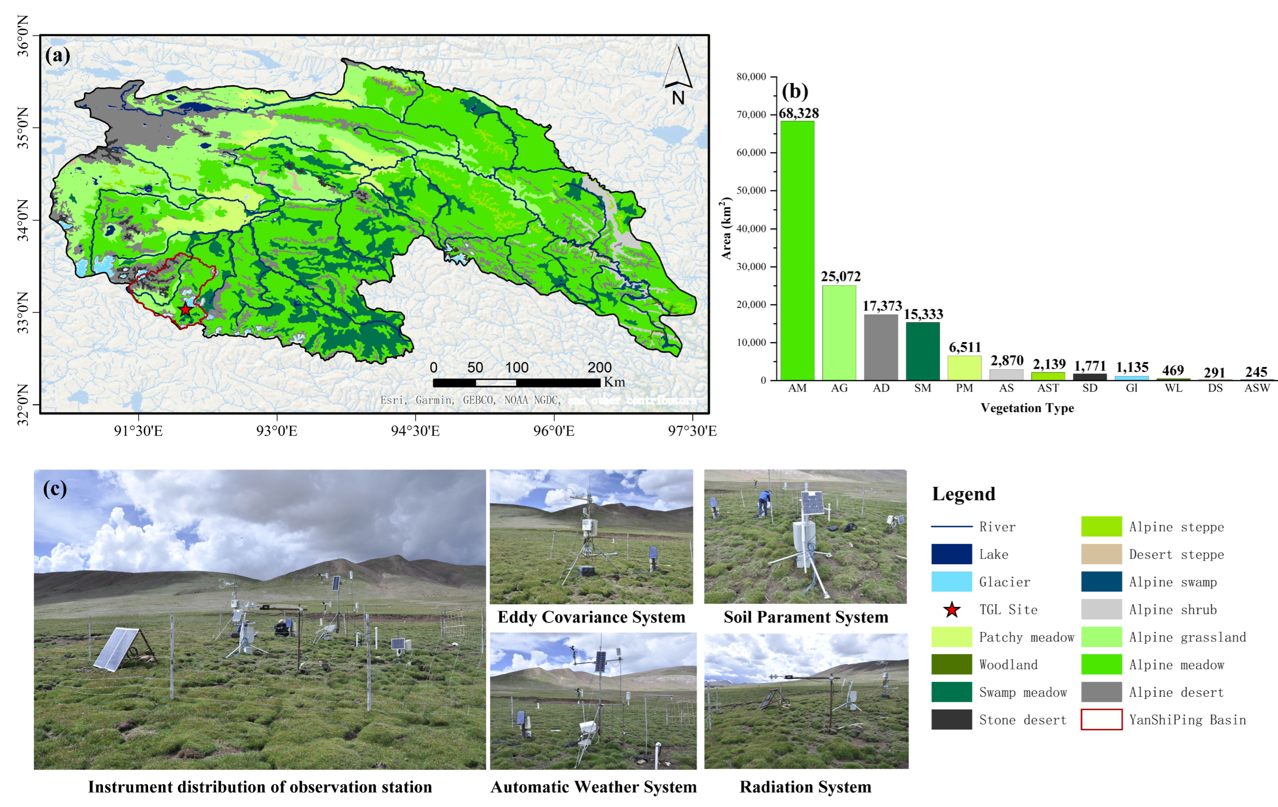
2.1. Study Area

About 11% of the vegetation types in the source region of the Yangtze River (SRYR) were alpine swamp meadow [26], but alpine swamp meadow has lacked the proper distinction from other alpine vegetations in past studies on evapotranspiration, which has impeded further research on its mechanism. Thus, according to the Vegetation Map of the People’s Republic of China, the vegetation types in the SRYR were clearly distinguished based on the dominant species and soil type, and the alpine swamp meadow was dominated by Kobresia littledalei and Carex moorcroftii (Figure 1a). The world’s first Eddy covariance system (Figure 1c) on the alpine swamp meadow above 5000 m was used to observe evapotranspiration at the Tanggula Mountain Cryosphere Hydrology and Ecology Field Scientific Experiment Station of the Chinese Academy of Sciences (TGL, 33°02′12.48″ N, 92°00′28.08″ E), which is located in the Dongkemadi River Basin in the source region of the Yangtze River on the central Tibetan Plateau. The orientation of the TGL is northeast to southwest (prevailing wind direction), so the areas covered by the Eddy covariance footprint (calculated by FFP) was a uniform alpine swamp meadow [27].

2.2. Data Acquisition and Processing

An integrated observation station was built at this site including an Eddy covariance system, meteorological system, and soil parameter system. The observation items and instruments, the data acquisition unit, and measurement height (depth) are listed in

Table 1. List of the observation items and instruments at the TGL site.

Observation Items		Sensor	Data Acquisition	Height/Depth
Eddy covariance system	3D wind velocity 3D wind direction	CSAT3, Campbell	CR1000	2.5 m
	Mixing ratio of water vapor	Li-7500, Campbell		2.5 m
Meteorological system	Wind velocity and direction	0513, R.M.Young	CR510X	1.5 m
	Air temperature	109, Campbell	CR510X	1.5 m
	Precipitation	T-200B, Geonor	CR1000	1.7 m
	Net radiation a	NR01, Hukseflux	CR1000	1.5 m
Soil parameter system	Soil moisture b and temperature	Hydra, Stevens	CR1000	0.1 m, 0.2 m, 0.3 m, 0.4 m 0.5 m, 0.7 m, 0.9 m, 1.1 m

Note(s): ^a Upward/downward shortwave radiation and upward/downward longwave radiation were measured separately. ^b Volumetric soil water content was measured and used to represent the soil moisture.

. Data from January to December 2020 were selected for research, and all data were resampled with a time resolution of 30 min.

2.2.1. Eddy Covariance System

The Eddy covariance method was coupled with the pulsation and vertical wind by covariance to compute the sensible heat flux H and latent heat flux λET_a:

$$H=\rho C_p\overline{{\omega }^{\prime }{\theta }^{\prime }}$$

(1)

$$\lambda E{T}_a=\lambda \rho \overline{{\omega }^{\prime }{q}^{\prime }}$$

(2)

where ρ is the density of air (kg/m³); C_p is the specific heat of air at constant pressure [(MJ/(kg·℃)]; λ is the latent heat of vaporization (MJ/kg); ω′ is the pulsation of the vertical component (m/s); θ′ is the pulsation of temperature (℃); and q′ is the pulsation of specific humidity (g/kg).

To ensure the accuracy of the results, raw data acquired at 10 Hz were processed using EddyPro (LI-COR, USA) including the spike removal, lag correction of H₂O relative to the vertical wind component, sonic virtual temperature correction, the performance of the planar fit coordinate rotation, corrections for density fluctuation (WPL-correction), and frequency response correction. Output flux data were conducted as follows: (i) data from periods of sensor malfunction were rejected; (ii) those within 1 h before and after precipitation were rejected; (iii) those missing more than 3% of raw data were rejected; (iv) data were rejected when the friction velocity was below 0.1 m/s, and after conducting the above procedure, about 71% of the flux data was available and quality flags were calculated for all fluxes; the flag values qc = 0 and qc = 1 for fluxes suitable for general analysis and qc = 2 for fluxes were discarded from the result dataset.

During long time observation, 17–50% of flux data were missing or rejected [28]. Liu used a look-up table (LUT) and mean diurnal variations (MDV) to fill the gap of flux data [3]. Xu indicated that LUT could obtain a better result when the meteorological observation data were available synchronously and MDV was more suitable for a short time gap-fill [29]. In this study, days of maximum continuous lack of data were less than 5 days; thus, LUT and MDV were required for the gap-fill and added with online flux data calculated by EasyFlux_DL (IRGASON, USA).

2.2.2. Meteorological System

The meteorological system included a two-layer gradient automatic weather system (GAWS) and a four-component radiation system. Wind speed (W_s) and direction (W_d) were measured at 1.5 m by Sensor-05103 (R.M. Young, USA). Mean air temperature (AT, °C) and relative humidity (RH, %) were measured at 1.5 m by a Sensor-109 (Campbell, USA). Precipitation (P, mm) was measured at 1.7 m using T-200B (Geonor, Norway) and the snow depth (S_dp, cm) was measured at 1.7 m by the snow-depth sensor and snow-pillow at the Earth’s surface. The net radiation (R_n, W/m²) was calculated from the downward/upward short-wave radiation and downward/upward long-wave radiation measured independently by NR01 (Hukseflux, The Netherlands) at a height of 1.5 m. It can be formulated as follows:

R_n = S_d − S_u + L_d − L_u

(3)

where S_d and S_u were the downward and upward short-wave radiation, and L_d and L_u were the downward and upward short-wave radiation, respectively. The unit of the above parameters was W/m².

All data were collected from the data acquisition unit by LoggerNet (Campbell, USA) and because the capture rates of solid and liquid precipitation are different, the precipitation data were corrected using a scheme in this area proposed by He [30].

2.2.3. Soil Parameter System

Soil parameters were measured at eight levels by HydraProbe (Stevens, USA) at a depth of 0.1–1.1 m, which include the volumetric soil water content (VSWC, m³/m³) and soil temperature (ST, °C). Additionally, the soil moisture and ST were used to calculate the soil heat flux (G, W/m²) using the thermal diffusion equation correction (TDEC) proposed by Yang [31], which has been well validated in a typical permafrost region of Naqu. The one-dimensional heat conduction equation of soil is as follows:

$$\frac{\partial {\rho }_s{\mathrm{c}}_{s}T}{\partial t}=-\frac{\partial G}{\partial z}$$

(4)

Integrating over both sides:

$$G(z)=G(z_r)+{\displaystyle \underset{Z_r}{\overset{Z}{\int }}\frac{\partial {\rho }_s{c}_{s}T(z)}{\partial t}}dz$$

(5)

Given the soil temperature profile T(Z_i), Equation (5) can be expressed as:

$$G(z)=G(z_r)+\frac{1}{\Delta t}{\displaystyle \sum _{Z_i}^Z\left[{\rho }_s{c}_s(Z_i,t+\Delta t)\cdot T_s(Z_i,t+\Delta t)-{\rho }_s{c}_s(Z_i,t)\cdot T_s(Z_i,t)\right]}$$

(6)

where ρ_sc_s is the soil heat storage [J/(kg·K)]; T_s is soil temperature (℃); t is the time (s); and G_z is the soil heat flux at a depth of z (W/m²) and G(Z_r) can be iterated from zero when the soil moisture and soil temperature observations are adequately deep. In this passage, we assumed that the soil heat conduction coefficient was 1.0 W/(m·k); subsequently, the soil diffusion equation was used to solve the temperature profile T(Z_i), and the observed temperature profile was used to correct it. Finally, Equation (6) was used to solve the soil heat flux of each layer, and the surface soil heat flux (G₀) was selected for future calculations.

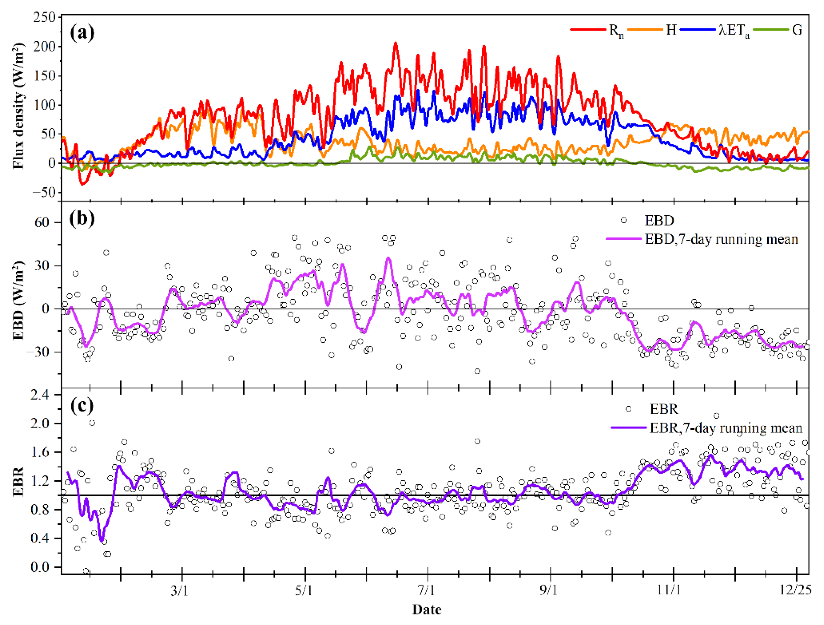
2.3. Energy Balance and Calculation of Evapotranspiration

The energy balance of an alpine swamp meadow is expressed as follows:

R_n = H +λET + G₀

(7)

As has been noted in the literature, the energy balance Equation (4) is not usually closed [29] The energy balance ratio (EBR) and energy balance deficit (EBD) were used to check the turbulence flux observation; this is expressed as follows:

$$EBR=\frac{{\displaystyle \sum (H+\lambda E)}}{{\displaystyle \sum (R_n-G})}$$

(8)

$$EBD=R_n-H-\lambda ET-G_0$$

(9)

In addition to the Eddy covariance to calculate the actual evapotranspiration (ET_a), the FAO Penman–Monteith Equation (FAO P–M; [21]) was used to calculate the reference crop evapotranspiration (ET₀), and the crop coefficient (K_c) at the alpine swamp meadow was calculated by comparing two approaches. The related formulas are expressed as follows:

$$E{T}_{0-daily}=\frac{0.408\Delta \left(R_n-G_0\right)+\gamma \frac{900}{T_a+273}{u}_2\left(e_s-e_a\right)}{\Delta +\gamma \left(1+0.34u_2\right)}$$

(10)

$$E{T}_{0-hourly}=\frac{0.408\Delta \left(R_n-G_0\right)+\gamma \frac{37}{T_a+273}{u}_2\left(e_s-e_a\right)}{\Delta +\gamma \left(1+0.34u_2\right)}$$

(11)

$$K_c=E{T}_a/E{T}_0$$

(12)

where Δ is the rate of change of saturation vapor pressure with temperature (kpa/℃); γis the psychrometric constant (kpa/℃); T_a is the air temperature at 2 m (℃); e_s and e_a represent the saturation vapor pressure at T_a and the actual air vapor pressure (kpa), respectively; and u₂ is the wind velocity at 2 m (m/s).

To calculate ET_a from ET₀ using a corrected K_c at the alpine swamp meadow, the root-mean-square error (RMSE) and Nash–Sutcliffe efficiency coefficient (NSE) were selected to evaluate the effectiveness of different approaches; their formulas are expressed as follows:

$$RMSD=[\frac{1}{n}{\displaystyle \sum _{i=1}^n(E{T}_{\mathrm{ec}(i)}}-{E{T}_{pm(i)})}^2{]}^{1/2}$$

(13)

$$NSE=1-\frac{{\displaystyle {\sum }_1^N{(E{T}_{\mathrm{ec}(i)}-E{T}_{pm(i)})}^2}}{{\displaystyle {\sum }_1^N{(E{T}_{pm(i)}-\overline{E{T}_{pm}})}^2}}$$

(14)

where ET_ec(i) indicates the actual evapotranspiration calculated by the Eddy covariance; ET_pm(i) is the actual evapotranspiration calculated by FAO P-M using the different K_c approach; and the overline denotes the average value.

2.4. Calculations of Parameters Influencing the Characteristics of Evapotranspiration

The daily equilibrium evapotranspiration (ET_eq, mm/d) and surface conductance g_s (ms⁻¹) were calculated from the Penman–Monteith equation using the following form [32]:

$$E{T}_{eq}=\frac{\Delta }{\Delta +\gamma }(R_n-G)$$

(15)

$$g_s^{-1}={\rho }_a{C}_{p}VPD/(\gamma \lambda E)+(\beta \Delta /\gamma -1)/g_a$$

(16)

where ET_eq (mm/d) is the evapotranspiration influenced only by radiative heating; ρ_a (kg/m³) is the moist air density; C_p [(MJ/(kg·℃)] is the specific heat of air at constant pressure; β is the Bowen ratio, which was computed by H/λE. The aerodynamic conductance g_a (m/s) was estimated from the friction velocity u_* (m/s) and wind speed u (m/s), and is expressed as:

$$g_a^{-1}=u/u_{*}^2+6.2u_{*}^{-0.67}$$

(17)

3. Result and Discussion

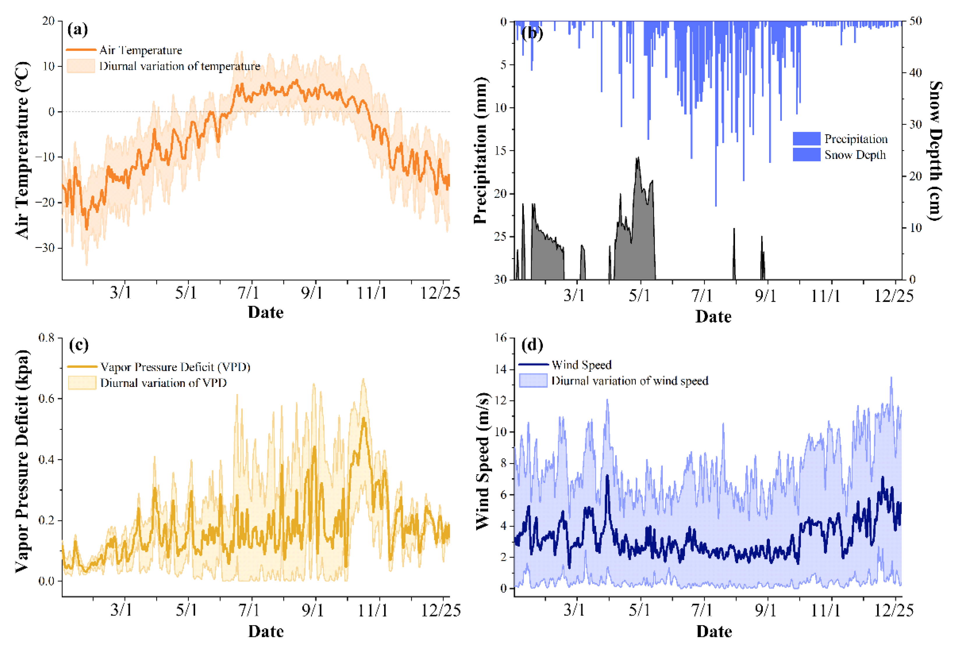
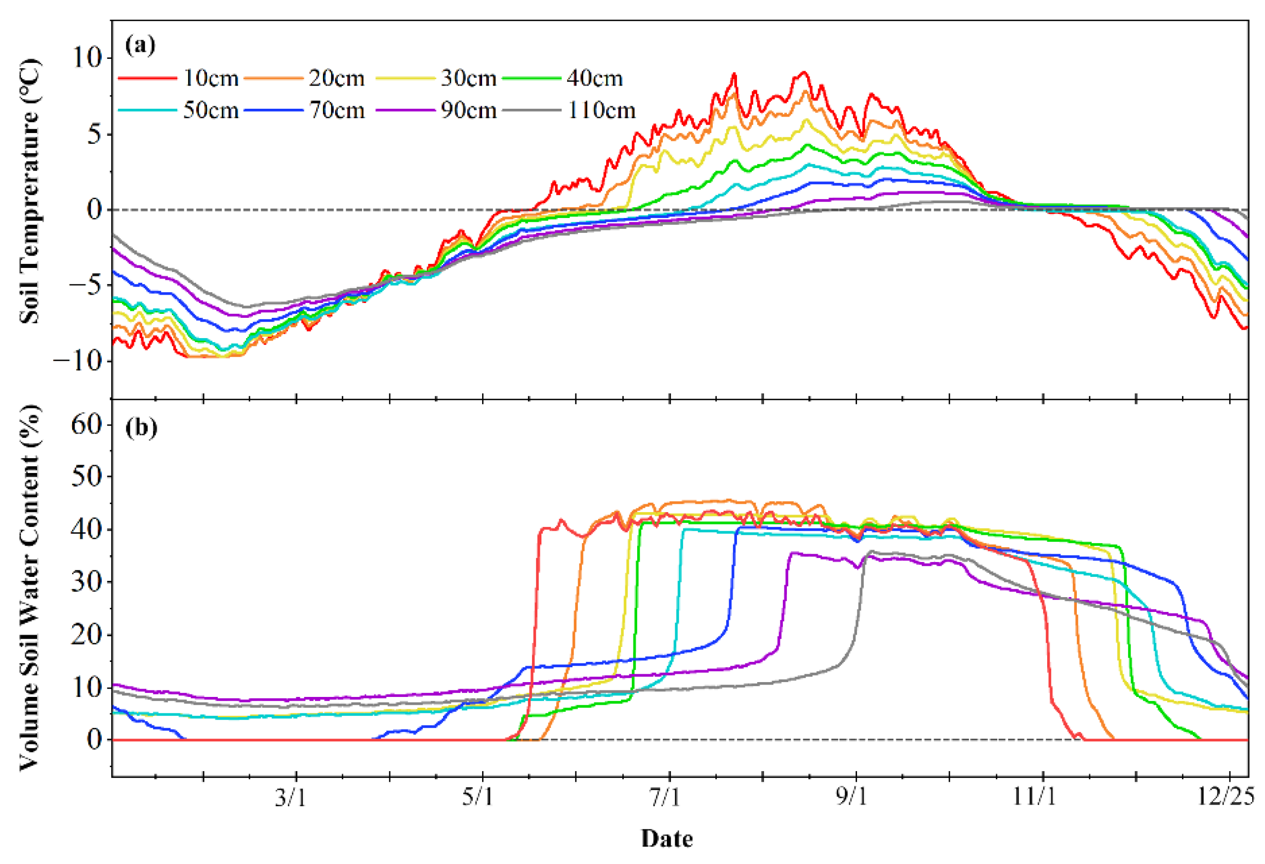
3.1. Characteristics of Environmental Elements

Meteorology, underlying surface, and radiation conditions are critical parameters affecting evapotranspiration. Therefore, the automatic meteorological system (AWS), soil parameter system, and radiation system of the TGL station was used to analyze the basic meteorological, underlying surface and radiation characteristics of the typical alpine swamp meadow and was the basis for subsequent research analysis. Figure 2 shows the variations in the meteorological conditions. The mean annual air temperature was −5.5 °C; the highest and lowest temperatures were 7.7 °C (9 August) and −26.96 °C (24 January), respectively. According to Wang [33], when the temperature was steady above 3 °C, the alpine swamp meadow entered the Ini-growing season. When the temperature was steady above 5 °C, the alpine swamp meadow entered the mid-growing season. When the temperature was steady under 5 °C but above 3 °C, the alpine swamp meadow entered the late-growing season. Thus, the Ini-growing season, mid-growing season, late-growing season were from 11 June–12 July, 13 July–15 August, and 16 August–21 September, respectively. The average wind speeds during the non-growing and growing seasons were 3.32 and 2.43 m/s, respectively, and the fluctuation was lower during the growing season. The mean values of the vapor pressure deficit (VPD) during the growing and non-growing seasons were 0.19 and 0.17 kpa, respectively. Precipitation occurred on 212 days throughout the year, with 741.7 mm of accumulated precipitation; the single maximum daily precipitation reached 21.4 mm (9 July). According to the snow depth sensor, solid precipitation was dominant in the non-growing season, and the snow-free period was from 13 May–31 December.

Figure 3 shows the variations in the ST and VSWC conditions. A distinct freezing–thawing cycle could be observed; the completely frozen stage (1 January–14 May) occurred when the ST was completely lower than 0 °C and the VSWC was stable. When the temperature of the surface soil was above 0 °C and the VSWC was saturated, the thawed stage began (2 September–27 October); when the VSWC increased, the thawing stage occurred (15 May–1 September); when the VSWC decreased, the freezing stage occurred (28 October–31 December).

Figure 4 shows the radiation condition and characteristics of the energy budget at this site. As the site is located at a high altitude, seasonal variation in the daily-mean net radiation (R_n) was significant, ranging from −32.64 to 222.77 W/m² (Figure 5a), and the annual average daily net radiation was 79.78 W/m². The maximum and minimum values occurred on 18 July–11 January, respectively. The average daily EBD and EBR were −2.47 W/m² and 1.078, respectively. Therefore, the energy balance in this site almost closed, and thus the λET values measured by the Eddy covariance system were considered reliable and the reason for the worse EBD and EBR values was the advection effect by the higher wind speed during the non-growing season.

3.2. Seasonal and Diurnal Variation of Evapotranspiration

Figure 5 shows the ET_a measured by the Eddy covariance system and reference evapotranspiration (ET₀) computed by the FAO P–M equation. ET_a and ET₀ had similar trends both on the day and annual scales, and all values showed unimodal variation (Figure 6a). ET_a was close to ET₀ during the growing season, but ET₀ was higher than ET_a during the freezing and completely frozen periods. ET₀ was higher than ET_a between 8:00 and 16:00 during the day, and the maximum ET₀ and ET_a values occurred at about 14:00 and 15:00, respectively. (Figure 5b). There was a hysteresis effect between the Eddy covariance and FAO Penman–Monteith methods and this phenomenon was also observed in an underlying surface with exposed water [34]. The ET_a measured by the Eddy covariance system indicated that nocturnal evapotranspiration existed at alpine swamp meadows, but the FAO P–M method underestimated it. Additionally, the nocturnal evapotranspiration phenomenon in the northern Utah region accounted for 1.7% of the total during a complete growing cycle of alfalfa [35]; that in the north Qinghai–Tibet Plateau region accounted for 9.8–15.8% from May to September in an alpine desert, alpine steppe, alpine meadow steppe, and alpine meadow [36], but the nocturnal evapotranspiration of alpine swamp meadows is still unclear.

Figure 6 shows the annual distribution of evapotranspiration. There was an obvious distribution characteristic: evapotranspiration after 12:00 accumulated 443.77 mm, and accounted for 78.3% of the annual actual evapotranspiration. Nocturnal evapotranspiration occurring during the growing season accumulated 63.45 mm, and accounted for 11.19% of the annual actual evapotranspiration.

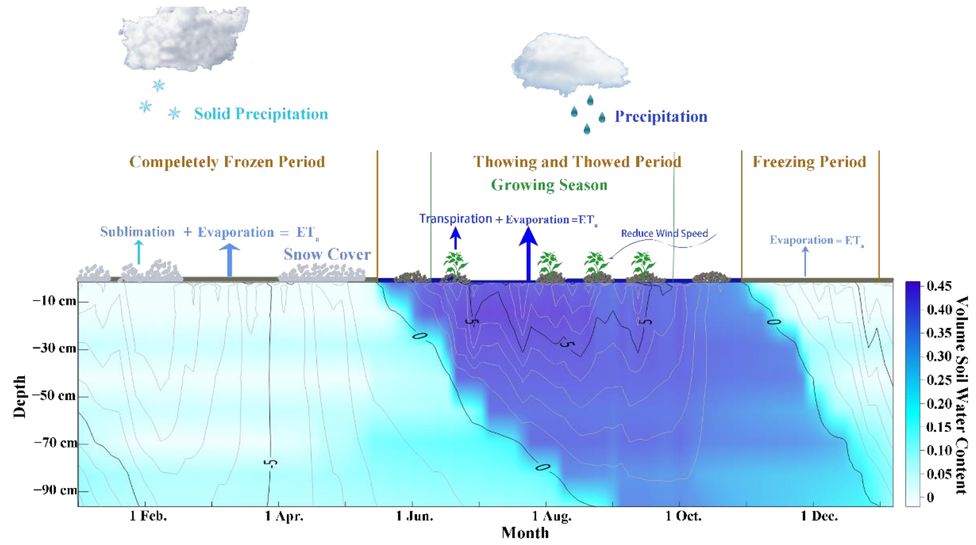
3.3. Hydrologic Balance

Figure 7 shows the seasonal variation in evapotranspiration and precipitation and its cumulative value in the alpine swamp meadow. During the period of observation, the cumulative precipitation (P_c) reached 741.7 mm, of which 476.3 mm occurred in the growing season, accounting for 64% of the annual precipitation (Figure 7a). The ratio of ET_a to P (ET_a/P) is an important parameter to depict the hydrological balance [37]. The annual actual evapotranspiration is 566.97 mm; thus, the annual ET_a/P was 0.76 and this value was close to that of an alpine steppe (0.51–0.77; [38]) but lower than that of a degraded alpine meadow (0.97; [37]). There were significant differences in the different periods. The ET_a/P values were 0.63 and 2.15 during the growing and during the non-growing seasons. Thus, from the ET_a/P, we inferred that the precipitation was recharged in air through evapotranspiration in the alpine swamp meadow; and in addition to precipitation, a mass of soil water entered the air through evapotranspiration during the non-growing season. Cumulative annual ET_eq (ET_eqc) and cumulative annual ET₀ (ET_0c) values were 917.50 and 889.84 mm, which were higher than the cumulative annual ET_a (ET_ac) and cumulative annual precipitation (P_c). The ET_eqc partly reflects the maximum possible evapotranspiration of an ecosystem influenced only by radiation [20], but the ET_0c was higher than ET_eqc before the growing season. Additionally, despite the marked increase in ET_eq and P_c during the growing season, there were no significant increases in ET_ac and ET_0c during the growing season. ET_eqc, P_c, and ET_ac were reduced, but ET_0c still had a rapid grow rate after the growing season (Figure 7b).

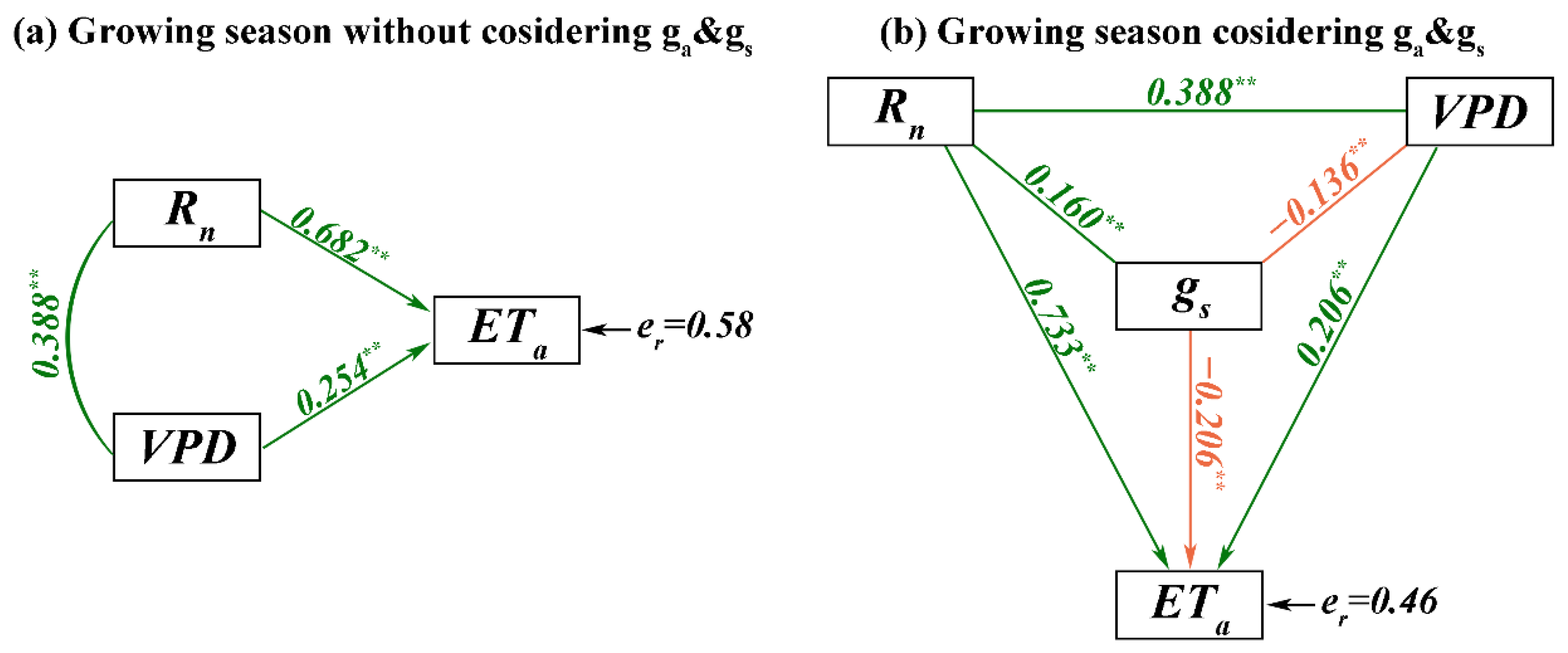
3.4. Relationship between Evapotranspiration and Environmental Elements

In this section, stepwise regression and path analysis were used to find the similarities and differences in the relationship between evapotranspiration and environmental elements during the growing and non-growing seasons.

Table 2. Results of the stepwise regression.

Period	Interpretation Equation	Adjust R2
Growing season	ETa = 0.696Rn + 0.247VPD	0.656
Non-growing season	ETa = 0.447VSWC a + 0.381Rn + 0.211ST a − 0.134P − 0.068Ws	0.793

Note(s): ^a Volume soil water content (VSWC) and soil temperature (ST) were selected as the average value of ground surface 0–10 cm.

presents the results of stepwise regression; we can recognize that the major influence factors during the growing season (MF_G) were the net radiation (R_n) and VPD, and those during the non-growing season (MF_NG) were the VSWC, net radiation (R_n), ST, P, and wind speed (W_s). The adjusted R² shows that the MF_G and MF_NG could explain about 66 and 79% of the evapotranspiration characteristics during the growing and non-growing seasons, respectively.

Figure 8 shows the structure of MF_G and MF_NG given by path analysis. The structure of MF_G and MF_NG given by path analysis reflects that the ET_a was mainly influenced by the radiation (R_n) and atmospheric (VPD) conditions during the growing season (Figure 8a); in addition to the radiation and atmospheric conditions, the soil condition also had a notable influence on the ET_a during the non-growing season. Evapotranspiration increased by 0.780 mm/d for every 1 W/m² increase in net radiation, wherein 0.682 mm/d was directly influenced by changes in the radiation condition and 0.098 mm/d occurred by the interaction between the radiation and atmospheric conditions (Path.1, Rn-VPD-ET_a: 0.098 mm/d) during the growing season (Figure 8a). Evapotranspiration increased by 0.749 mm/d for every 1 W/m² increase in net radiation, wherein 0.381 mm/d was directly influenced by changes in the radiation condition, 0.382 mm/d was through the positive interaction between the radiation and soil conditions (Path.1, Rn-VSWC-ET_a: 0.242 mm/d; Path.2 Rn-ST-ET_a: 0.119 mm/d; Path.3 Rn-Ws-ET_a: 0.021 mm/d), and −0.015 mm/d was through the negative interaction between the radiation and atmospheric conditions (Path.1 Rn-P-ET_a:−0.015 mm/d) during the non-growing season (Figure 8b).

From the above relationship, we inferred that ET_a was restrained when precipitation occurred during the non-growing season because the solid precipitation blocked the water exchange between the air and ground surface. Soil conditions were no longer major factors influencing the ET_a at the alpine swamp meadow during the growing season because the soil surface water content had already saturated during the onset of the growing season; this also explained why the jump in precipitation had not brought notable changes in the ET_a. This conclusion was similar to that of Zhang, who highlighted that the positive effect between VSWC and ET_a was stronger during drought [39]. Although the results of stepwise regression show that the direct effect of wind speed on evapotranspiration is negative (path.1 Ws-ET_a), the combined effect exerted by other environmental elements through wind speed increases the actual evapotranspiration (e.g., Path1.R_n-W_s-ET_a).

As presented in Table 2 and shown in Figure 8a, regardless of whether the adjusted R² was lower or e_r was higher during the growing season, other factors influenced the ET_a. Burenina et al. pointed out that the characteristics of evapotranspiration is determined by the general climatic characteristics of the research area and different species composition [40]. Thus, the surface conductance g_s and aerodynamic conductance g_a were incorporated into the path analysis model to evaluate the influence of the alpine swamp meadow on evapotranspiration. The results shown in Figure 9 indicate that after considering factor g_s, which represents the effect of vegetation, the adjusted R² and e_r increased from 0.656 to 0.790 and 0.56 to 0.46, respectively. Although g_s had a negative relationship with ET_a, the effect of g_s was two-sided: one way was evapotranspiration influenced by the increase in atmospheric conditions from 0.519 to 0.547 mm/d for every 1 kpa increase in VPD (Path.1 VPD-g_s-ET_a), and another way is evapotranspiration influenced by the change in radiation conditions from 0.780 to 0.747 mm/d for every 1 W/m² increase in net radiation (Path.1 Rn-g_s-ET_a). This may partly explain why the ET_eqc had a more rapid growth rate than that of ET_ac during the growing season in Figure 7b.

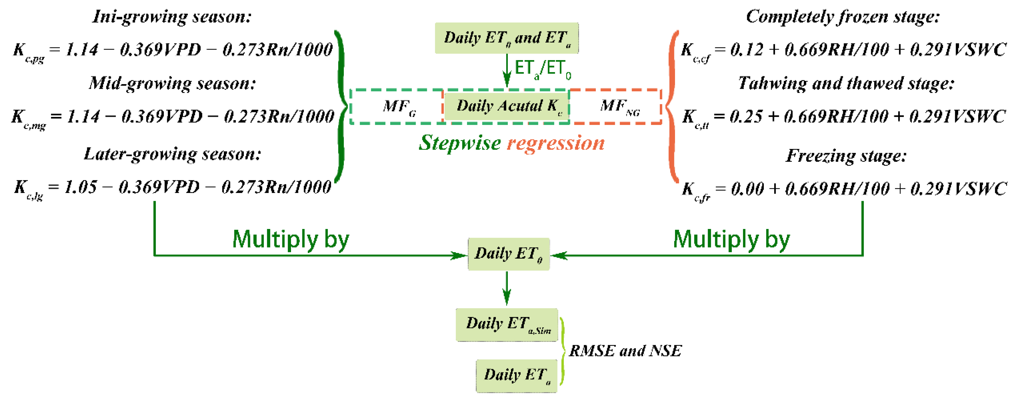
3.5. A New Correct Scheme of Crop Coefficient

Figure 10 shows the process of evapotranspiration at the alpine swamp meadow. Obvious thawing and freezing processes and exposed water existed during the growing season, thereby leading to a unique evapotranspiration process in the alpine swamp meadow. Thus, we inferred that the reason for a significantly higher ET₀ than ET_a during the thawed and completely frozen periods is that the FAO P–M only uses radiation and atmospheric conditions to calculate evapotranspiration without sufficiently considering the influence of freeze–thaw cycle to evapotranspiration, and the crop coefficient recommended by the FAO also does not fully consider the impact of the freeze–thaw process. Thus, the crop coefficient (K_c) requires a new correction scheme when using the FAO P–M in the alpine swamp meadow with an obvious freeze–thaw cycle.

Figure 11 shows the parameterization schemes of K_c and the result for the correction of K_c by initially calculating the actual K_c by ET_a/ET₀. Additionally, MF_G and MF_NG were used to build the regression equation between the daily actual K_c and to ensure the accuracy of K_c; the piecewise function was established according to the vegetation growth stage and freeze–thaw process. The new K_c was multiplied with the daily ET₀ to obtain the daily ET_a calculated by ET₀ (ET_a,Sim). The results showed that the foundation coefficients were between 0 and 0.25 and 1.05 and 1.14 during the non-growing and growing seasons, respectively, and the VSWC was found to be the key parameter in the model during the non-growing season. The modified crop coefficients take into account VSWC to reflect the effects of the freeze–thaw processes on evapotranspiration and can improve the computational accuracy of models for evapotranspiration. The correction scheme proposed in this paper can not only obtain the actual evapotranspiration in the growing season by ET₀, but also obtain the actual evapotranspiration in the non-growing season by calculating the crop coefficient by VSWC and RH.

Figure 12 shows the corrected result and ET_a measured by the Eddy covariance system. The annual ET_a calculated by ET₀ was 592.34 mm, which was 25.37 mm larger than the ET_a. The NSE of the scheme was 0.87 and the RMSE of the scheme was 0.44 mm/d; thus, this scheme could effectively evaluate the ET_a of the alpine swamp meadow. Moreover, we also calculated ET_a through the FAO-recommended Kc [21], whose values are as follows: K_c,ini = 0.4; K_c,mid = 1.05 + K_c,FAO; K_c,later = 0.85 + K_c,FAO. The related formula is expressed as:

$$K_{c,FAO}=K_{c,recommend}+[0.04(u_2-2)-0.004R{H}_{\min }-45]{(\frac{h}{3})}^{0.3}$$

(18)

where h is the canopy height of the alpine swamp meadow (m).

The result showed that the FAO-recommended K_c underestimated the ET_a at the Ini-growing season and was similar to the corrected results during mid- and later-growing seasons. The main reasons why the FAO recommended factors underestimate the actual evapotranspiration during the Ini-growing season are: (1) the growth characteristics of alpine swamp meadow are not a perfect match with the reference crops; (2) dramatic changes in soil water content caused by permafrost freeze–thaw cycles and surface micro-fluctuations in alpine swamp meadow cause the aerodynamic resistance and canopy surface resistance to differ significantly from the reference crops (Jia et al., 2014). This new corrected scheme error mainly occurs in the following ways:

• By providing less consideration to parameters and using a one-dimensional linear relationship;
• The soil water content of an alpine swamp meadow is high, and the enthalpy of water leads to a phase difference between the ET_a and ET₀ calculated by FAO P–M [34].

4. Conclusions

The annual correction coefficient of the FAO P–M formula was obtained through comparative observations based on the clear evapotranspiration characteristics and influencing factors of an alpine swamp meadow. Thus, it can be better applied in an alpine swamp meadow area, and our conclusions are as follows:

(1)

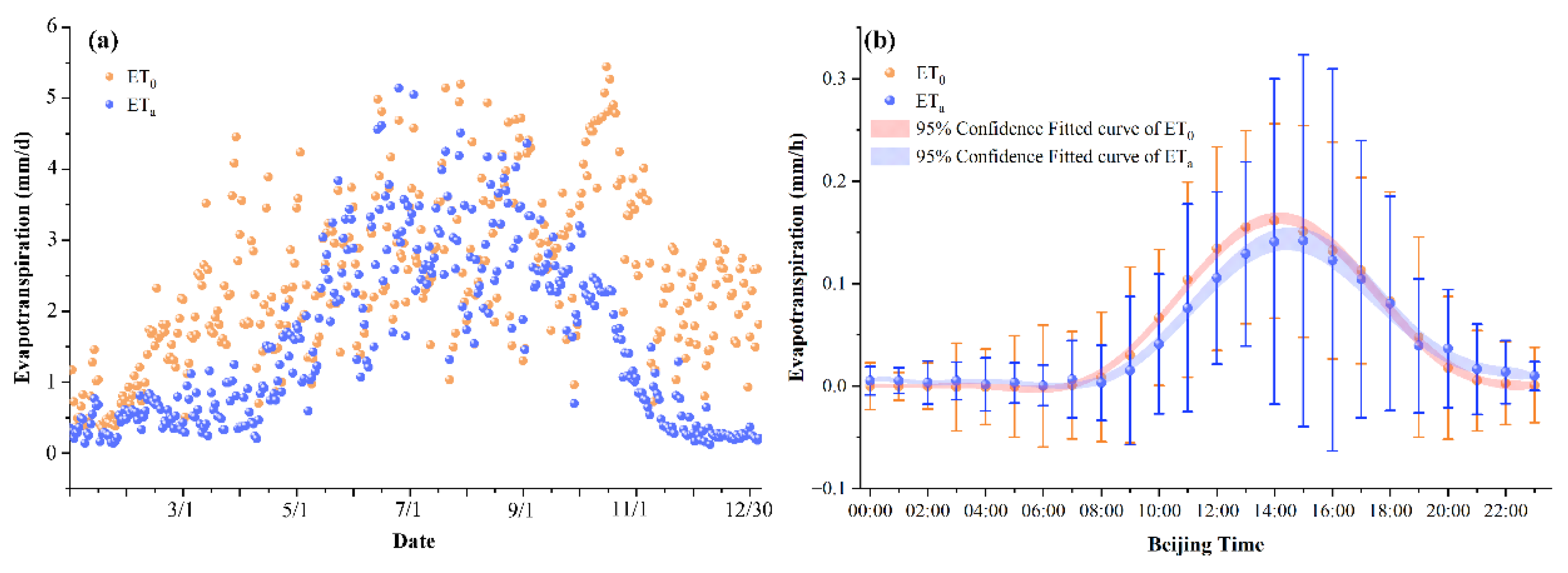
ET_a measured by the Eddy covariance system and ET₀ calculated by FAO P–M showed the same trend on the daily and annual scales, where all values showed unimodal variation, and hysteresis was confirmed between ET₀ and ET_a. Therefore, ET_a can be calculated by ET₀ for alpine swamp meadow, but the error due to hysteresis should be considered in subsequent studies.

(2)

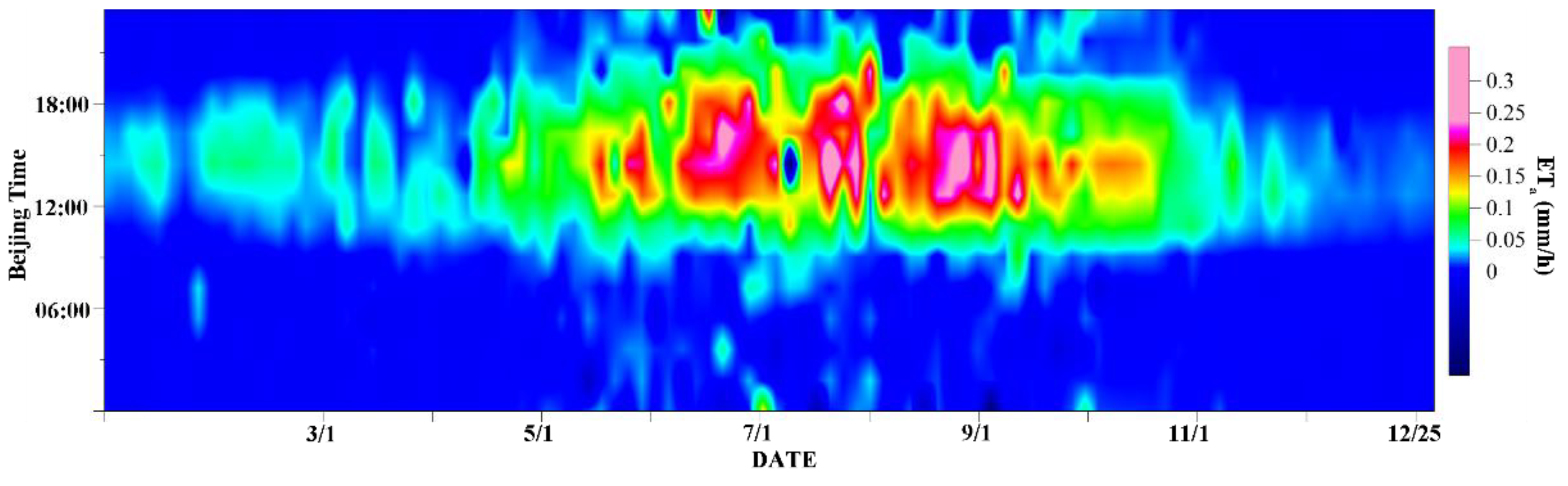
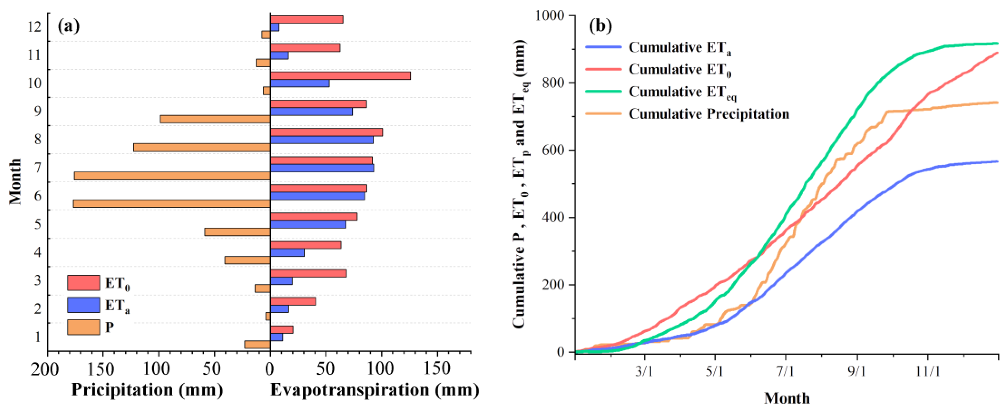
The hydrological balance of alpine swamp meadow was different from that of an alpine steppe and alpine meadow, where the annual ET_a and annual ET_a/P were 566.97 mm and 0.76, with about 11.19% of ET_a occurring at night. The ET_a during non-growing seasons was 2.15, implying that a large amount of soil water was released into the air by evapotranspiration, and whether is this the cause of alpine meadow degradation also remains to be investigated.

(3)

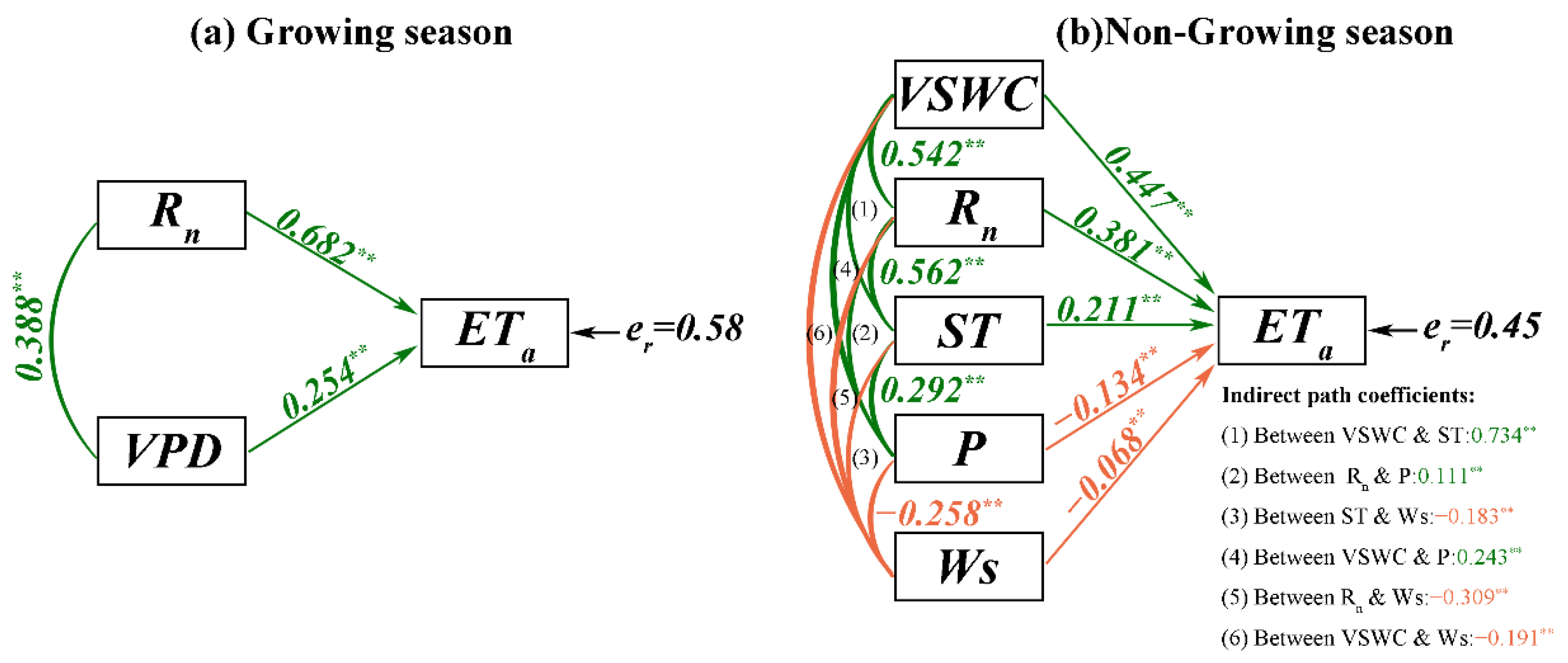
The main influencing factors during the growing season were R_n, VPD, and g_s, and the main influencing factors during the non-growing season were VSWC, Rn, ST, P, and W_s. Therefore, the evapotranspiration characteristics of an alpine swamp meadow are formed under the following conditions: control of net radiation, affected by VPD during the growing season and affected by soil temperature and humidity during the non-growing season. Precipitation and soil water content are no longer the main controlling factors of evapotranspiration during the growing season at an alpine swamp meadow as the volume soil water content tends to saturate.

(4)

The basic corrected K_c was 1.14 during the initial and mid-growing season, 1.05 during the later growing season, and 0–0.25 during the non-growing season. Moreover, not only can this corrected crop coefficient effectively calculate the actual evapotranspiration from ET₀ of the alpine swamp meadow, the correction factor process can also provide ideas for correcting the Kc of other vegetation. In fact, in this paper, we only corrected the single-crop coefficients, which could not separate vegetation transpiration and evaporation. Therefore, the segmentation of transpiration and evaporation in alpine swamp meadow is still worth further discussion.

References

1. Wu, J.; Chen, J.; Qin, Y. Comparative Study of Evapotranspiration in an Alpine Meadow in the Upper Reach of Shulehe River Basin. Sci. Geogr. Sin. 2013, 33, 97–103. [Google Scholar]
2. Oliver, H.R.; Oliver, S.A. The Role of Water and the Hydrological Cycle in Global Change; Springer: Berlin/Heidelberg, Germany, 1995. [Google Scholar]
3. Liu, S.; Xu, Z.; Zhu, Z.; Jia, Z.; Zhu, M. Measurements of evapotranspiration from eddy-covariance systems and large aperture scintillometers in the Hai River Basin, China. J. Hydrol. 2013, 487, 24–38. [Google Scholar] [CrossRef]
4. Wang, R.; Li, L.; Gentine, P.; Zhang, Y.; Chen, J.; Chen, X.; Chen, L.; Ning, L.; Yuan, L.; Lü, G. Recent increase in the observation-derived land evapotranspiration due to global warming. Environ. Res. Lett. 2022, 17, 024020. [Google Scholar] [CrossRef]
5. Zhu, B.; Zhang, Q.; Yang, J.-H.; Li, C.-H. Response of Potential Evapotranspiration to Warming and Wetting in Northwest China. Atmosphere 2022, 13, 353. [Google Scholar] [CrossRef]
6. Azam, F.; Farooq, S. Agriculture and Global Warming: Evapotranspiration as an Important Factor Compared to CO2. Pak. J. Biol. Sci. 2005, 8, 1630–1638. [Google Scholar] [CrossRef] [Green Version]
7. Jung, M.; Reichstein, M.; Ciais, P.; Seneviratne, S.I.; Sheffield, J.; Goulden, M.L.; Bonan, G.; Cescatti, A.; Chen, J.; de Jeu, R.; et al. Recent decline in the global land evapotranspiration trend due to limited moisture supply. Nature 2010, 467, 951–954. [Google Scholar] [CrossRef] [Green Version]
8. Liu, Z. Estimating land evapotranspiration from potential evapotranspiration constrained by soil water at daily scale. Sci. Total Environ. 2022, 834, 155327. [Google Scholar] [CrossRef]
9. Lewis, C.S.; Allen, L.N. Potential crop evapotranspiration and surface evaporation estimates via a gridded weather forcing dataset. J. Hydrol. 2017, 546, 450–463. [Google Scholar] [CrossRef] [Green Version]
10. Wang, H.; Zhang, M.; Cui, L.; Yu, X. Spatial Heterogeneity in Sensitivity of Evapotranspiration to Climate Change. Polish J. Environ. Stud. 2017, 26, 2287–2293. [Google Scholar] [CrossRef]
11. Su, T.; Feng, G.L. Spatial-temporal variation characteristics of global evaporation revealed by eight reanalyses. Sci. China-Earth Sci. 2015, 58, 255–269. [Google Scholar] [CrossRef]
12. Fisher, J.B.; Melton, F.; Middleton, E.; Hain, C.; Anderson, M.; Allen, R.; McCabe, M.F.; Hook, S.; Baldocchi, D.; Townsend, P.A.; et al. The Future of Evapotranspiration: Global requirements for ecosystem functioning, carbon and climate feedbacks, agricultural management, and water resources. Water Resour. Res. 2017, 53, 2618–2626. [Google Scholar] [CrossRef]
13. Yao, T.; Bolch, T.; Zhao, P. The imbalance of the Asian water tower. Nat. Rev. Earth Environ. 2022, 3, 1–15. [Google Scholar] [CrossRef]
14. Peng, J.; Liu, Z.; Liu, Y.; Wu, J.; Han, Y. Trend analysis of vegetation dynamics in Qinghai-Tibet Plateau using Hurst Exponent. Ecol. Indic. 2012, 14, 28–39. [Google Scholar] [CrossRef]
15. Zhou, D.; Hao, L.; Kim, J.B.; Liu, P.; Pan, C.; Liu, Y.; Sun, G. Potential impacts of climate change on vegetation dynamics and ecosystem function in a mountain watershed on the Qinghai-Tibet Plateau. Clim. Change 2019, 156, 31–50. [Google Scholar] [CrossRef]
16. Chen, B.; Luo, S.; Lü, S.; Zhang, Y.; Di, M. Effects of the soil freeze-thaw process on the regional climate of the Qinghai-Tibet Plateau. Clim. Res. 2014, 59, 243–257. [Google Scholar] [CrossRef]
17. Cheng, G.; Wu, T. Responses of permafrost to climate change and their environmental significance, Qinghai-Tibet Plateau. J. Geophys. Res.-Earth Surf. 2007, 112. [Google Scholar] [CrossRef] [Green Version]
18. Zeng, C.; Zhang, F.; Joswiak, D.R. Impact of alpine meadow degradation on soil hydraulic properties over the Qinghai-Tibetan Plateau. J. Hydrol. 2013, 478, 148–156. [Google Scholar] [CrossRef]
19. Nistor, M.M.; Cheval, S.; Gualtieri, A.F.; Dumitrescu, A.; Boţan, V.E.; Berni, A.; Hognogi, G.; Irimuş, I.A.; Porumb-Ghiurco, C.G. Crop evapotranspiration assessment under climate change in the Pannonian basin during 1991–2050: Climate change effects on crop evapotranspiration, Pannonian basin. Meteorol. Appl. 2017, 24, 84–91. [Google Scholar]
20. Wu, H.T.; Zhu, W.W.; Huang, B. Seasonal variation of evapotranspiration, Priestley-Taylor coefficient and crop coefficient in diverse landscapes. Geogr. Sustain. 2021, 2, 224–233. [Google Scholar] [CrossRef]
21. Allan, R.; Pereira, L.; Smith, M. Crop Evapotranspiration-Guidelines for Computing Crop Water Requirements-FAO Irrigation and Drainage Paper 56; Utah State University: Logan, UT, USA, 1998. [Google Scholar]
22. Ragab, R.; Evans, J.G.; Battilani, A.; Solimando, D. Towards Accurate Estimation of Crop Water Requirement without the Crop Coefficient Kc: New Approach Using Modern Technologies. Irrig. Drain. 2017, 66, 469–477. [Google Scholar] [CrossRef] [Green Version]
23. Ma, N.; Zhang, Y. Increasing Tibetan Plateau terrestrial evapotranspiration primarily driven by precipitation. Agric. For. Meteorol. 2022, 317, 108887. [Google Scholar] [CrossRef]
24. Jia, Z.-J.; Han, L.; Wang, G.; Zhang, T.-S. Adaptability analysis of FAO Penman-Monteith model over typical underlying surfaces in the Sanjiang Plain, Northeast China. Chin. J. Appl. Ecol. 2014, 25, 1327–1334. [Google Scholar]
25. Wang, G.; Li, Y.; Wang, Y.; Shen, Y. Impacts of alpine ecosystem and climate changes on surface runoff in the headwaters of the Yangtze River. J. Glaciol. Geocryol. 2007, 29, 159–168. [Google Scholar]
26. Wang, Z.-W.; Wang, Q.; Zhao, L.; Wu, X.-D.; Yue, G.-Y.; Zou, D.-F.; Nan, Z.-T.; Liu, G.-Y.; Pang, Q.-Q.; Fang, H.-B.; et al. Mapping the vegetation distribution of the permafrost zone on the Qinghai-Tibet Plateau. J. Mt. Sci. 2016, 13, 1035–1046. [Google Scholar] [CrossRef]
27. Kljun, N.; Calanca, P.; Rotach, M.W.; Schmid, H.P. A simple two-dimensional parameterisation for Flux Footprint Prediction (FFP). Geosci. Model Dev. 2015, 8, 3695–3713. [Google Scholar] [CrossRef] [Green Version]
28. Falge, E.; Baldocchi, D.; Olson, R.; Anthoni, P.; Aubinet, M.; Bernhofer, C.; Burba, G.; Ceulemans, R.; Clement, R.; Dolman, H.; et al. Gap filling strategies for defensible annual sums of net ecosystem exchange. Agric. For. Meteorol. 2011, 107, 43–69. [Google Scholar] [CrossRef] [Green Version]
29. Xu, Z.; Liu, S.; Tongren, X.; Jiemin, W. Comparison of the Gap Filling Methods of Evapotranspiration Measured by Eddy Covariance System. Adv. Earth Sci. 2009, 24, 372–382. [Google Scholar]
30. He, X.B.; Ye, B.S.; Ding, Y.J. Bias correction for precipitation mesuament in Tanggula Mountain Tibetan Plateau. Adv. Water Sci. 2009, 20, 403–408. [Google Scholar]
31. Yang, K.; Wang, J. A temperature prediction correction method for calculating surface soil heat flux based on soil temporature and humidity data. Sci. China Press 2008, 38, 243–250. [Google Scholar]
32. Monteith, J.I.L. Evaporation and Environment. Symp. Soc. Exp. Biol. 1965, 19, 205–234. [Google Scholar]
33. Wang, L.; He, X.; Ding, Y. Characteristics and influence factors of the evapotranspiration from alpine meadow in central Qinghai-Tibet Plateau. J. Glaciol. Geocryol. 2019, 41, 801–808. [Google Scholar]
34. Cui, Y.; Liu, Y.; Gan, G.; Wang, R. Hysteresis Behavior of Surface Water Fluxes in a Hydrologic Transition of an Ephemeral Lake. J. Geophys. Res. -Atmos. 2020, 125, e2019JD032364. [Google Scholar] [CrossRef]
35. Malek, E. Night-time evapotranspiration vs. daytime and 24h evapotranspiration. J. Hydrol. 1992, 138, 119–129. [Google Scholar] [CrossRef]
36. Liao, Q.; Li, X.; Shi, F.; Deng, Y.; Wang, P.; Wu, T.; Wei, J.; Zuo, F. Diurnal Evapotranspiration and Its Controlling Factors of Alpine Ecosystems during the Growing Season in Northeast Qinghai-Tibet Plateau. Water 2022, 14, 700. [Google Scholar] [CrossRef]
37. Zhang, L.-F.; Zhang, J.-Q.; Zhang, X.; Liu, X.-Q.; Zhao, L.; Li, Q.; Chen, D.-D.; Gu, S. Characteristics of Evapotranspiration of Degraded Alpine Meadow in the Three-River Source Region. Acta Agrestia Sin. 2017, 25, 273–281. [Google Scholar]
38. Gu, S.; Tang, Y.; Cui, X.; Du, M.; Zhao, L.; Li, Y.; Xu, S.; Zhou, H.; Kato, T.; Qi, P.; et al. Characterizing evapotranspiration over a meadow ecosystem on the Qinghai-Tibetan Plateau. J. Geophys. Res. -Atmos. 2018, 113, D08118-1–D08118-10. [Google Scholar] [CrossRef]
39. Zhang, H.; Dou, R.Y. Interannual and seasonal variability in evapotranspiration of alpine meadow in the Qinghai-Tibetan Plateau. Arab. J. Geosci. 2020, 13, 968. [Google Scholar] [CrossRef]
40. Burenina, T.; Danilova, I.; Mikheeva, N. Spatial-Temporal Dynamics of Evapotranspiration in the Podkamennaya Tunguska River Basin. Contemp. Probl. Ecol. 2022, 15, 449–458. [Google Scholar] [CrossRef]
Figure 1. (a) Map of the vegetation type of the source region of the Yangtze River (SRYR), which is located in in the interior Qinghai–Tibet Plateau (QTP). [Editorial Board of Vegetation Map of China, Chinese Academy of Sciences, 2001]. (b) Proportion of vegetation and underlying surface types in the SRYR: AM, Alpine meadow; AG, Alpine grassland; AD, Alpine desert; SM, Swamp meadow; PM, Patchy meadow; AS, Alpine shrub; AST, Alpine steppe; SD, Stone desert; Gl, Glacier; WL, Woodland; DS, Desert steppe; ASW, Alpine swamp. (c) Distribution of instruments of the observation station and photos of the Eddy covariance system, soil parameter system, automatic weather system, and radiation system.
Water 14 03578 g001
Figure 2. Variations in the (a) air temperature (AT) at a height of 2 m; (b) precipitation (bar) and snow depth (shaded graph); (c) vapor pressure deficit (VPD) at 2 m; and (d) wind speed (WS) at 2.5 m. All data are 30-min averages and (a) air temperature, (b) wind speed, and (c) VPD are shown with their respective daily maximums and minimums. The light color divides the growing season and non-growing periods.
Water 14 03578 g002
Figure 3. Variations in the (a) soil temperature (ST) and (b) volumetric soil water content (VSWC) at depths of 0.1 to 1.1 m, respectively.
Water 14 03578 g003
Figure 4. Variations in the (a) flux density at a height of 2 m, (b) energy balance deficit (EBD), and (c) energy balance ratio (EBR); the purple and pink solid lines represent 7-day running mean values, and others represent the daily mean value.
Water 14 03578 g004
Figure 5. Variations in the (a) daily average evapotranspiration; the red squares represent the reference evapotranspiration (ET0) and blue hollow circles represent the actual evapotranspiration (ETa); (b) hourly average evapotranspiration; the red squares represent the reference evapotranspiration (ET0), blue hollow circles represent the actual evapotranspiration (ETa), the red shadow represents the fitted curve of ET0 under a 95% confident level, the blue shadow represents the fitted curve of ETa under a 95% confident level, and error bars denote the standard deviation of hourly data.
Water 14 03578 g005
Figure 6. The annual distribution of evapotranspiration at the alpine swamp meadow during 2020. The different colors from blue to pink represent the actual evapotranspiration (ETa) per half hour. The time between 6:00 and 18:00 represents daytime.
Water 14 03578 g006
Figure 7. (a) Seasonal variation in evapotranspiration and precipitation in the alpine swamp meadow. (b) Cumulative reference evapotranspiration (ET0c), cumulative actual evapotranspiration (ETac), cumulative equilibrium evapotranspiration (ETeqc), and cumulative precipitation (Pc).
Water 14 03578 g007
Figure 8. The structures of MFG and MFNG given by path analysis during the (a) growing season and (b) non-growing season. One-way influence was shown with arrows; the interplay of environmental elements is represented by the line without arrows. Additionally, the green and orange colors implied positive and negative relationships between the actual evapotranspiration (ETa) and environmental elements, respectively. er indicates that the residual error was calculated by er = (1-R2)1/2. The asterisk superscript implies that the value passed the 95% significance t-test.
Water 14 03578 g008
Figure 9. (a) The structure of MFG and MFNG given by path analysis without considering ga and gs during the growing season; and (b) that while considering ga and gs during the growing season. One-way influence was denoted by arrows; the interplay of environmental elements was represented by a line without arrows. Additionally, green and orange colors implied positive and negative relationships between the actual evapotranspiration (ETa) and environmental element. er indicates that the residual error was calculated by er = (1 − R2)1/2. The asterisk superscript implies that the value passed the 95% significance t-test.
Water 14 03578 g009
Figure 10. The process of evapotranspiration at the alpine swamp meadow; the bottom half refers to the VSWC and ST; ST and VSWC are denoted by contours and color strips, respectively. The upper half shows the condition of the underlying surface. The arrow implies evapotranspiration from the surface and the dark blue underlying surface represents the exposed water.
Water 14 03578 g010
Figure 11. Correction and parameterization schemes of Kc; rectangle with rounded corners and green background implies the used or calculated data. Green arrow implies the processing of data and the dashed rectangle implies the stepwise regression between the data and main influencing factors. Brace represents the result. ETa,Sim represents the actual evapotranspiration calculated by the reference evapotranspiration.
Water 14 03578 g011
Figure 12. The corrected ETa (little red square) calculated by ET0 compared with the ETa (blue line) measured by the Eddy covariance system and ETa (gray hollow circle) calculated by the FAO-recommended Kc.
Water 14 03578 g012