
A Hydrograph-Based Approach to Improve Satellite-Derived Snow Water Equivalent at the Watershed Scale

Département de Génie Civil et de Génie du Bâtiment, Université de Sherbrooke, Sherbrooke, QC J1K 2R1, Canada
*
Author to whom correspondence should be addressed.
Water 2022, 14(21), 3575; https://doi.org/10.3390/w14213575
Submission received: 7 October 2022
/
Revised: 1 November 2022
/
Accepted: 2 November 2022
/
Published: 7 November 2022
(This article belongs to the Section Hydrology)
Abstract
:For the past few decades, remote sensing has been a valuable tool for deriving global information on snow water equivalent (SWE), where products derived from space-borne passive microwave radiometers are favoured as they respond to snow depth, an important component of SWE. GlobSnow, a novel SWE product, has increased the accuracy of global-scale SWE estimates by combining remotely sensed radiometric data with other physiographic characteristics, such as snow depth, as quantified by climatic stations. However, research has demonstrated that passive microwaves algorithms tend to underestimate SWE for deep snowpack. Approaches were proposed to correct for such underestimation; however, they are computer intensive and complex to implement at the watershed scale. In this study, SWEmax information from the near real time 5-km GlobSnow product, provided by Copernicus and the European Space Agency (ESA) and GlobSnow product at 25 km resolution were corrected using a simple bias correction approach for watershed scale applications. This method, referred to as the Watershed Scale Correction (WSC) approach, estimates the bias based on the direct runoff that occurs during the spring melt season. Direct runoff is estimated on the one hand from SWEmax information as main input. Infiltration is also considered in computing direct runoff. An independent estimation of direct runoff from gauged stations is also performed. Discrepancy between these estimates allows for estimating the bias correction factor. This approach is advantageous as it exploits data that commonly exists i.e., flow at gauged stations and remotely sensed/reanalysis data such as snow cover and precipitation. The WSC approach was applied to watersheds located in Eastern Canada. It was found that the average bias moved from 33.5% with existing GlobSnow product to 18% with the corrected product, using the recommended recursive filter coefficient β of 0.925 for baseflow separation. Results show the usefulness of integrating direct runoff for bias correction of existing GlobSnow product at the watershed scale. In addition, potential benefits are offered using the recursive filter approach for baseflow separation of watersheds with limited in situ SWE measurements, to further reduce overall uncertainties and bias. The WSC approach should be appealing for poorly monitored watersheds where SWE measurements are critical for hydropower production and where snowmelt can pose serious flood-related damages.
1. Introduction
Hydrological processes for watersheds located in northern latitudes and at high elevations are greatly affected by seasonal snowfall. Spring snowmelt is arguably one of the most important processes for operational hydrology of these territories, as it is a critical component for determining flood risk [1]. However, the prediction of spring snowmelt is contingent on having accurate estimates of the amount of liquid water stored in the snowpack, i.e., snow water equivalent (SWE), and more particularly, the maximum snow water equivalent (SWEmax) before the onset of snowmelt. This is especially true for effective management of water resources and for predicting spring floods over large watersheds where spring snowmelt may last for extended periods and where there is a delay between the occurrence of SWEmax and peak flow. Additionally, accurate estimates of SWE are important ecologically in terms of water availability. This is so because groundwater replenishment depends on the amount of snowmelt and unusually low SWEmax will affect summer low flows [2].
SWE, including SWEmax, are traditionally estimated from manual point snow surveys. These surveys are limited in their spatial (i.e., individual observation points) and temporal coverage (i.e., typically only begins once the snowpack is considered well developed) and, therefore, do not always well represent watershed state [3]. For smaller and more homogeneous environments, the interpolation of spatially sparse point snow observations from either snow courses or weather stations may be adequate for estimating SWE and SWEmax at the watershed scale. However, for larger and more heterogeneous watersheds, alternative methods are needed in order to capture the high spatial (and temporal) variability of the snowpack, combined with terrestrial heterogeneity, and therefore, estimate SWE and SWEmax at the watershed scale.
Passive microwave (PM) sensors have been used for decades to improve the spatial coverage of SWE estimates. These sensors quantify the brightness temperature naturally emitted from Earth across the microwave wavelengths and can be used to estimate SWE because snow grains of a developed snowpack scatters microwave radiation as it is transmitted through the snowpack [4]. This method has three main limitations Firstly, the microwave brightness temperature decreases as the snowpack gets deeper [5]. This methodology is limited to dry snow conditions, as wet snow is opaque to microwaves and the quantified microwave radiation originates from a thin layer at the top of the snowpack [6]. Secondly, this methodology underestimates SWE under deep snow conditions (i.e., when SWE exceeds approximately 150 mm). The main reason is that higher brightness temperature values are recorded as snow absorbs radiation from the bottom layer and emits a signal stronger than that of dry snow covering soil, which is not properly accounted for [7]. The exact limit depends on snowpack stratigraphy and grain size. Thirdly, Space-borne microwave radiometers, like the Advanced Microwave Scanning Radiometer-EOS (AMSR-E) and the Special Sensor Microwave Imager/Sounder (SSMI/S) provide SWE estimates with full spatial coverage under dry snow conditions. However, these estimates suffer issues related to the coarse spatial resolution of these sensors (approximately 25 km2). Snowpack properties are highly variable at spatial scales smaller than the satellites’ footprint (<25 km2), driven by changes in vegetative and topographic controls [4,8], this fine-scale heterogeneity results in measurement errors in SWE estimates. Therefore, stand-alone algorithms for these PM observations can be suitable for mesoscale to continental scale applications but may not provide sufficient accuracy at the watershed scale for operational hydrology application [9], save for very large watersheds.
Methods that combine remote sensing with ground-based measurements, for example, the algorithm in described in Pulliainen [10], can help overcome limitations of either method alone and have further improved SWE estimates. Pullianinen’s algorithm combines passive microwave radiometer data with ground-based synoptic snow depth observations in the Helsinki University of Technology (HUT) snow emission model to estimate SWE [11]. The algorithm first solves the HUT model using weather station measurements of snow depth to obtain effective snow grain size by fitting simulated to observed satellite brightness temperature measurements at the locations of weather stations. This information is then interpolated to a 25 km × 25 km pixel resolution and used in an assimilation procedure for estimating SWE [10]. GlobSnow applies this approach using PM data from Nimbus-7 Scanning Multichannel Microwave Radiometer (SMMR), The Defense Meteorological Satellite Program (DMSP) SSM/I and DMSP SSMI/S to produce a 25-km SWE product over the Northern hemisphere, as described in Takala et al. [12] and Luojus et al. [11]. Further refinement to the original GlobSnow dataset uses land cover/land use data [13] to downscale SWE estimates to a 5-km product, which is available in near-real time.
With these advances, the GlobSnow SWE product is at a spatial resolution appropriate for hydrological applications at the watershed scale; however, limitations regarding the issue of SWE underestimation in deeper snowpack remains. Several methods have been proposed to reduce the bias with some success, such as explicitly considering snowpack stratification in the microwave emission model [11,14] and assimilating PM data into a microwave emission model using snow grain size simulated by a physically based snowpack model [14]. However, these approaches are complex to implement operationally and, therefore, there is a need for a simple bias correction approach that can provide SWE and SWEmax estimates at the watershed scale. The Watershed Scale Correction (WSC) approach proposed here aims to correct the underestimation of spatially varying SWE, including SWEmax, produced by GlobSnow, at the watershed scale. This approach innovatively applies historical streamflow measurements and, thus, can be applied even if there are no available ground-based snow measurements. To do so, runoff water volumes retrieved from streamflow gauge stations are compared with the volumes resulting from SWEmax of GlobSnow, and then corrected based on the volumetric difference. The functionality of the approach is demonstrated by comparing the corrected SWE values with those obtained from snow course measurements at selected watersheds of varying sizes in the province of Québec, Canada.
2. Materials and Methods
2.1. WSC Overview
The WSC approach aims to improve the accuracy of the SWEmax of regional databases, such as GlobSnow V3 [11] using streamflow information. The approach was coded in MATLAB.
The motivation behind the WSC approach is that the watershed surface runoff originating from snowmelt, along with any precipitation during the spring snowmelt period, will eventually leave the watershed through its outlet. This approach focuses on direct runoff (i.e., total runoff minus baseflow) instead of looking at total runoff. According to the mass balance equation applied at the watershed scale, the direct runoff calculated from the amount of snow over the watershed, referred to as DRG (Direct Runoff using GlobSnow), should be equal to DRH, the direct runoff hydrograph retrieved from measured streamflow, which is:
DRH = DRG
However, given that SWEmax from GlobSnow is typically underestimated, it is likely that DRG be less than DRH. To remove this bias, an adjustment is applied to GlobSnow’s SWEmax, according to the following equation:
where, is the SWEmax estimated from GlobSnow, is the corrected SWEmax, and CF is the correction factor value. Note that a single CF value is applicable to the entire watershed, while SWEmax (both corrected and GlobSnow) is spatially distributed.
The estimation of DRG and DRH can be done using the following equations:
where, ROtotal is the total runoff estimated from the streamflow hydrograph, B is the baseflow, I is the infiltration, P is the total precipitation occurring during the snowmelt period, and A is the watershed surface area.
Combining Equations (1)–(4), one obtains the equation for CF:
Given that is typically underestimated, DRG is likely less than DRH, and therefore CF will be larger than 1.
Recall that a single CF value is applicable to the entire watershed, while SWEmax (either corrected or GlobSnow) is spatially distributed. A CF value should be computed for each year, where a spring runoff hydrograph is available. Therefore, it is expected that no single CF value will characterize a watershed for the following reasons:
- is derived using the HUT model. GlobSnow V1 and V2 [12] assume that the snowpack is made of a single homogeneous layer, while V3 [11] represents the snowpack as a stacked system of snow layers. Despite this improvement over the original HUT model, uncertainties in SWEmax estimation remain, especially when the snowpack undergoes multiple freeze-thaw and rain-on snow events, which will be reflected by changing CF values.
- Because of the limited penetration depth of the PM signal, it is expected that the CF will be larger when deeper snowpack conditions are encountered.
- Flow measurements also have errors related to the rating curve used to convert stream water level into streamflow.
- Finally, other sources of uncertainty related to precipitation, baseflow, and infiltration estimates will also affect CF.
Therefore, the proposed WSC approach is likely to provide a range of CF values. Although this might raise questions regarding how to select the ‘best’ CF value for correcting SWE, when the approach is applied to flood forecasting, the range of CF values is compatible and may be seen as reflecting the various sources of uncertainties affecting SWE estimation.
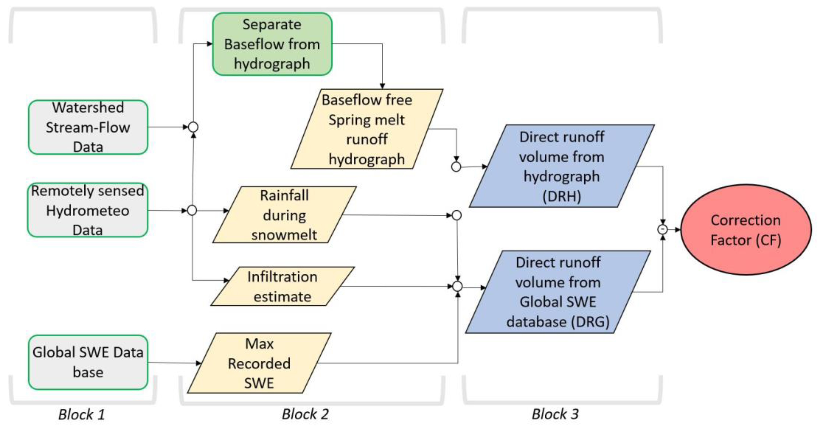
The WSC method can be divided into three main blocks as depicted in Figure 1. The first block relates to the organisation and retrieval of data, based on the watershed’s location. Each watershed is characterized by its own hydrometeorological regime and state variables (e.g., streamflow, precipitation, temperature, and SWE).
The second block uses the information obtained in Block 1 to estimate watershed state variables and hydrological processes required to compute DRG and DRH, and ultimately the correction factor (as shown in Block 3). Watershed state variables include SWEmax from the GlobSnow database and the duration of the snowmelt period, defined as the difference between the time SWEmax occurs and when the snow has disappeared. Both state variables can be retrieved from time series of SWE provided by the GlobSnow database. Alternatively, snow cover area obtained from ERA5 land cover product, based on information from MODIS datasets, can be used to establish the last day where there is snow in a watershed, and therefore to estimate the duration of the snowmelt period. Watershed hydrological processes include precipitation during the snowmelt period, watershed infiltration and baseflow. Once the duration of the snowmelt period is established, the total precipitation (rain and snow) occurring during this period can be retrieved. Baseflow separation and watershed infiltration methods used here are briefly described below.
Baseflow separation. Baseflow separation was performed using the HydRun tool box [15], a nested group of functions used for rapid and flexible rainfall-runoff analysis. The package, written in MATLAB, allows computing baseflow (Bt) and direct runoff (qt) from total runoff Qt, see Equations (6) and (7) below. The baseflow is computed using the recursive digital filter technique proposed by Nathan and McMahon [16]:
where is the baseflow at time t, is the direct runoff, represents the original streamflow and , is a filter coefficient which affects the magnitude of the baseflow values. For example, increasing produce a lower baseflow. Researchers used prescribed values for to obtain optimal results [17,18]. Gan and Zuo [17] set the value between the range 0.90–0.95, whereas Mau and Winter [18] used 0.85 for best results. Nathan and McMahon [16] suggested that the optimal value should be 0.925. It is advised to thoroughly investigate the value depending on the hydro-geological conditions in the catchment. To facilitate baseflow separation, the software also offers options to preprocess the hydrograph, such as hydrograph filtering establishing the maximum tolerable difference of discharge between the start and finish of an event and discarding peaks lower than a threshold value, allowing small fluctuations to be ignored while computing Bt.
The toolbox is effective for analysis of rainfall-generated hydrographs but presents some uncertainty as it remains to be tested for hydrographs generated by snowmelt [15]. However, other studies have applied the digital recursive method of separation to areas with snow cover [17,19,20,21]. While Hammond and Kampf [19] and Fan et al. [21] used β = 0.925 as the optimal filtering parameter value as suggested by previous studies [16,20], baseflow separation is highly sensitive to the filtering parameter and heuristic baseflow separation should be done with care, as true values of baseflow in snow-dominated systems are seldom available for optimizing the filtering parameter value [20].
As an alternative to observed baseflow values, Ref. [17] simulated baseflow in glacier melt dominated basins using the SWAT hydrological model and compared these ‘observations’ with baseflow produced according to the recursive filter method with β = 0.925. They found that the recursive filtering method produced flows comparable to SWAT during the low-flow period but overestimated baseflow in the high-flow method. Therefore, for the catchments examined here we chose a range of values from 0.800–0.995, with one run including the suggested optimal value, as it will be seen/discussed later.
Infiltration. Frozen ground is common to northern regions and infiltration of meltwater into frozen ground is a complex process that involves exchange of heat and mass flow with phase change [22]. To estimate DRG (see Equation (4)), it is required to estimate the amount of water infiltrating into frozen ground. According to Nicholaichuk and Gray [23], infiltration of snowmelt into frozen ground involves three possible water transfer and storage conditions depending on the surface entry conditions for the study area: restricted, unlimited, and limited. Restricted and unlimited water flows result in most all, or no snowmelt being infiltrated, respectively. In contrast, limited water flows result in some snowmelt being infiltrated and is influenced primarily by the soil physical properties, such as the available water storage capacity. Gray et al. [22] describe an algorithm that calculates areal infiltration into frozen ground on a watershed or hydrological response unit that combines the above three infiltration conditions. For each landscape unit in the watershed, the fraction classified as unlimited, restricted and limited infiltration varies dynamically according to the water holding capacity of frozen soil and cumulative infiltration is computed accordingly.
The equation used to quantify the Infiltration for frozen, unsaturated soils of limited infiltrability is described as:
where INF if the cumulative infiltration (mm), S0 is the soil moisture content at the soil surface, C is the land cover type coefficient, t0 is the infiltration opportunity time (h), SI and TI are the average soil saturation (mm3/mm3) and temperature (K), respectively, of the first 40-cm soil layer at the start of infiltration. S0 is usually taken as 1 due to low infiltration rate for frozen soil in areas where snow ablates rapidly. For prairie land covers C is 2.10, while for the forest covers it is 1.14.
The variable t0 is the time it takes for the snow cover to completely melt assuming that the melt is continuous, there is a small storage space, and little evaporation [22]. The following equation was used to estimate the t0:
Here, we assumed that limited infiltration conditions prevail during the snowmelt period and, accordingly, Equation (8) was used to calculate total infiltration into frozen soil. Note that depending on the value taken by SI, which is the soil saturation at the onset of the snowmelt, solving Equation (8) would result in restricted infiltrability if the soil is completely saturated (SI = 1, therefore INF = 0) and unlimited infiltrability would result as SI = 0. Further information on the infiltration into frozen ground algorithm is given in Gray et al. [22] and in Zhao and Gray [24].
Figure 2 proposes a linear relationship between CF and SWE. As mentioned above, CF corrects for the bias in estimates based on the direct runoff that occurs during the spring melt season. The same correction factor cannot be applied to correct observations during the winter season, which presents SWE information when SWE is below SWEmax. Previous research e.g., [25,26,27] has shown that PM starts underestimating SWE under deep snow conditions. It is therefore conceivable that the CF factor should vary between 1 (no correction) when SWE is above a certain threshold value, called SWEthres, and CFmax, the correction factor corresponding to SWEmax.
Whether or not this linear relationship holds true would require a detailed analysis of GlobSnow derived SWE against ground measurements. Nevertheless, for simplicity a linear relationship was applied here and provided reasonable estimates of corrected SWE values when compared against observed ground measurements (see result section for details). Here, we calculated CF only during the build-up of the snowpack. Initially, we defined SWEthresh as 150 mm following Luojus et al. [27] However, we observed that some years GlobSnow reported values of SWEmax below 150 mm and our associated CF values were smaller than 1 suggesting that SWEthresh should be smaller than 150 mm. This is in line with Larue et al. [7] in their analysis of GlobSnow data in Eastern Canada, who observed that PM SWE starts to be underestimated at depths above 100 mm. Accordingly, we defined SWEthresh value as 100 mm.
2.2. Study Area
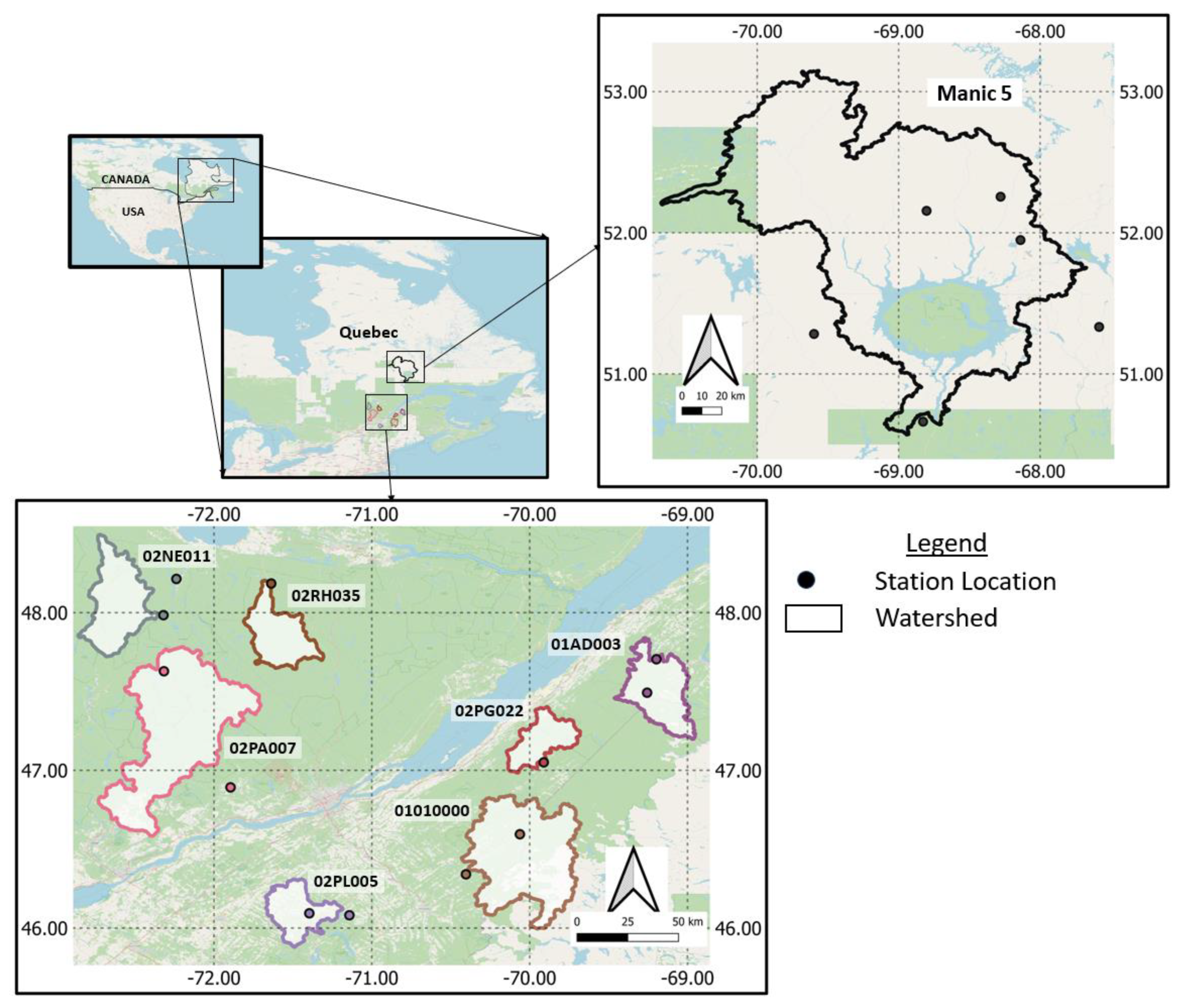
The study was conducted on eight watersheds located in south central Quebec, Canada, between 50 to 54° N latitude and 67 to 70° W longitude, see Figure 3. All watersheds have natural flows, except for the Manic 5 watershed, which has regulated flows. The watersheds’ areas vary from 795 km2 (02PG022—Ouelle River Watershed) to 24,698 km2 (Manic 5 watershed), see Table 1. All watersheds are mostly forested; for example, forests in 02PA007 (Batiscan River) and Manic 5 watersheds occupy respectively 87 and 83% of the total surface area. The remaining landcover is characterized as either open water (including wetlands), agricultural, or urban areas; for example, 14% of Manic 5 watershed consists of open water and wetlands, while only 7% of 02PA007 watershed is open water and wetlands. The Manic 5, 02RH035 (Aux Écorces River), 02NE011 (Croche River), and 02PA007 watersheds are in the Canadian Shield, which is characterized by small lakes and rolling hills as the result of glacial erosion from the last ice age. 02PL005 (Upper Bécancour River), 01010000 (St-John River), 01AD003 (St-Francis), and 02PG022 watersheds are located in the Appalachian Region of Eastern Canada, which is characterized by rolling hills and mountains. These watersheds are characterized by heavy winter snowfall and snowmelt runoff in the spring. Average maximum snow water equivalent (SWE) varies from 217 mm for 02PL005 watershed up to 298 mm for 02RH035 watershed, and generally increases from south to north because of lower air temperature with increasing latitude. Annual peak flow predominantly occurs during the spring thaw. The Manic 5 watershed, the largest in size and with heavy snowpack, has mean annual discharge is 529 m3/s [28] and annual peak flows exceeding on average 2000 m3/s, occurring in May. SWE can reach values of 300 mm or more [29]. Flow from Manic 5 drains into a 2000 km2 hydropower reservoir, with an installed capacity of 2.6 GW [30].
Hydrometeorological information about these watersheds can be found in Table 1.
2.3. Data
2.3.1. GlobSnow
The GlobSnow V3 SWE dataset, as described in Luojus et al. [11], was selected for analysis. The product combines passive microwave radiometer data from Nimbus-7 Scanning Multichannel Microwave Radiometer (SMMR), the Special Sensor Microwave Imager/Imager (SSM/I) and the Special Sensor Microwave Imager/Sounder (SSMIS) Defense Meteorological Satellite Program (DMSP), along with ground based synoptic snow depth observations using Bayesian data assimilation in the HUT snow emission model [11]. The algorithm first solves the HUT model using weather station measurements of snow depth to obtain effective snow grain size by fitting simulated to observed satellite brightness temperature measurements at the locations of weather stations. This information is then interpolated to a 25 km × 25 km grid cell and used in an assimilation procedure for the estimation of SWE [10,27]. Takala et al. in their study [32] applied a two-dimensional convolution window of 0.25° × 0.25° (25 km × 25 km) to change the calculation grid to 0.05° (approximately 5 km) projected in EASE-grid. The 25-km gridded GlobSnow product is available from 1979 to present. The 5-km product is available from 2006 to present and provides daily SWE 12 h after global satellite data has been acquired [33]. According to Luojus et al. [11], the 25-km product has an overall root mean square error (RMSE) for shallow to moderate snowpack (SWE < 150 mm) of 32.7 mm for the period covering 1980–2016 with no apparent bias but uncertainty increases when SWE is above this threshold.
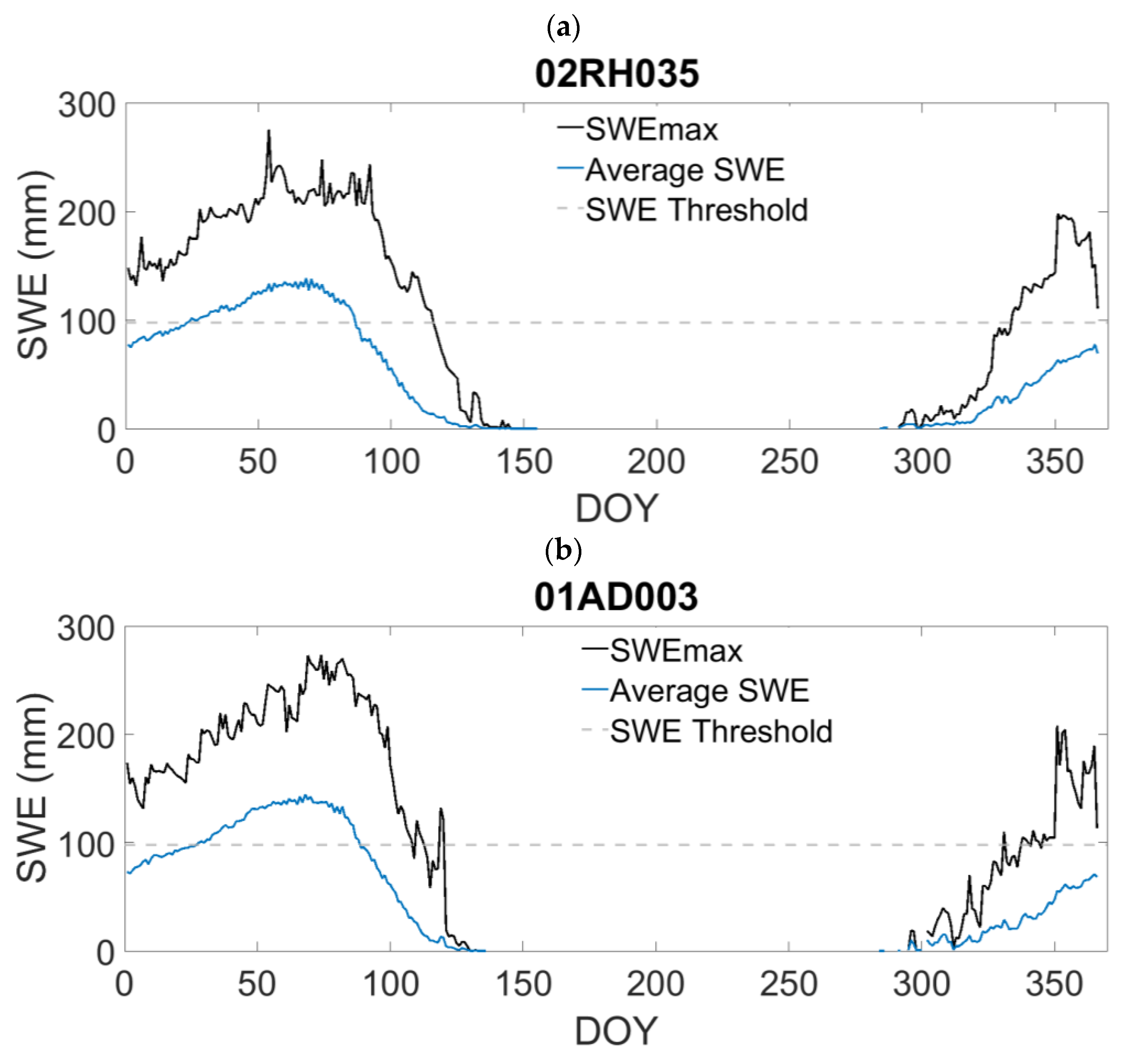
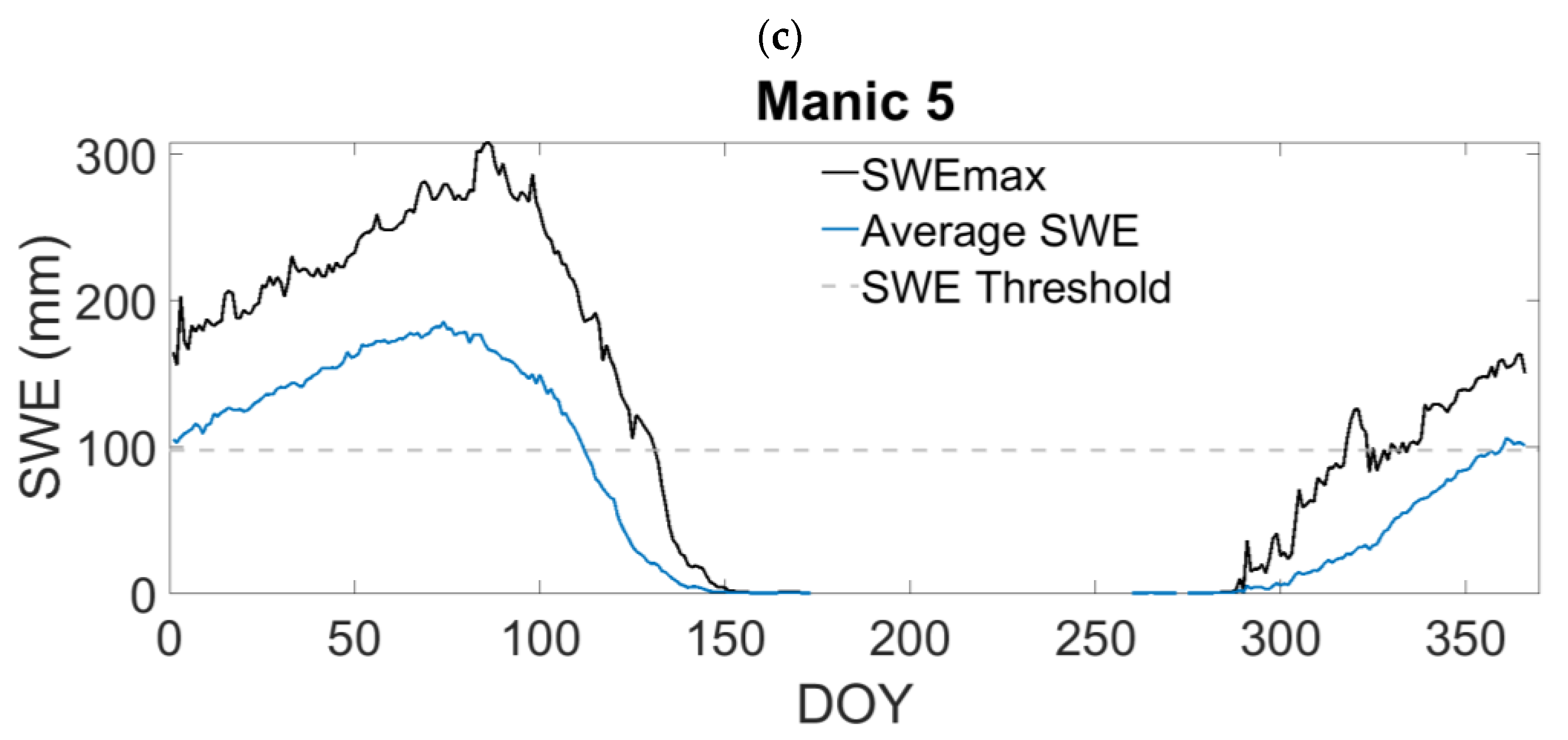
We retrieved the SWE information for the study watersheds from the GlobSnow database. Figure 4 illustrates the temporal evolution of SWE for three watersheds, namely 02RH035 (Rivière des Écorces), 01AD003 (St-Francis River), and Manic 5. The temporal coverage, average SWEmax from GlobSnow and from ground observations for the watersheds illustrated in Figure 4 along with other study sites are presented in Table 2, showing that GlobSnow underestimates SWE compared to in situ measurements.
2.3.2. ERA5
The fifth-generation European Centre for Medium- Range Weather Forecasts (ECMWF) atmospheric Reanalysis of global climate (ERA5) database provides hourly data estimates at a resolution of approximately 31 km for the global atmosphere, land surface, and ocean waves from 1950 to present. We used ERA5 to obtain the average soil saturation (SI) and temperature (TI) required as input for the Gray’s infiltration model. Compared to its predecessor ERA-interim, ERA5 has been greatly improved [34]. Improvements of the land surface model of ERA5 include a point wise simplified extended Kalman filter for three soil moisture layers in the top 1 m of soil, and a one-dimensional optimal interpolation for soil temperature [35]. Additional improvements of ERA5 are explained in detail by Hersbach et al. [36].
2.3.3. Streamflow Data
We used streamflow information from the Hydrometeorological Sandbox—École de technologie supérieure (HYSETS), a comprehensive dataset containing daily hydrometeorological data for over 14,400 watersheds across north America [31]. Streamflow information includes station location, flow regime (i.e., natural or regulated), daily flow data, as well as maximum and minimum daily air temperature and precipitation weather gauges, along with the SWE of ERA5-land. The database includes data covering the period 1950–2018 depending on the type and source of data. The streamflow data in HYSETS were retrieved from national water agencies repositories. For our study watersheds, streamflow is collected by Water Survey Canada (WSC) and stored in the National Water Data Archive (HYDAT). Further details on the HYSETS configuration are given in Arsenault et al. [31].
2.3.4. In Situ Data
The in situ SWE data, which from hence forth will be used interchangeably with the term ‘reference SWE data’, comes from Hydro-Québec’s (HQ) snow course measurements for Manic 5 watershed and from Québec’s Ministère de l’Environnement et de la Lutte contre les changements climatiques (MELCC) for the remaining watersheds investigated in this study. The SWE measurements are the average value of 10 samples equally spaced along a 300-m snow course [29]. These measurements are usually taken biweekly once the snowpack is developed until the snowmelt begins. The location of the measurement sites is depicted in Figure 3.
3. Results
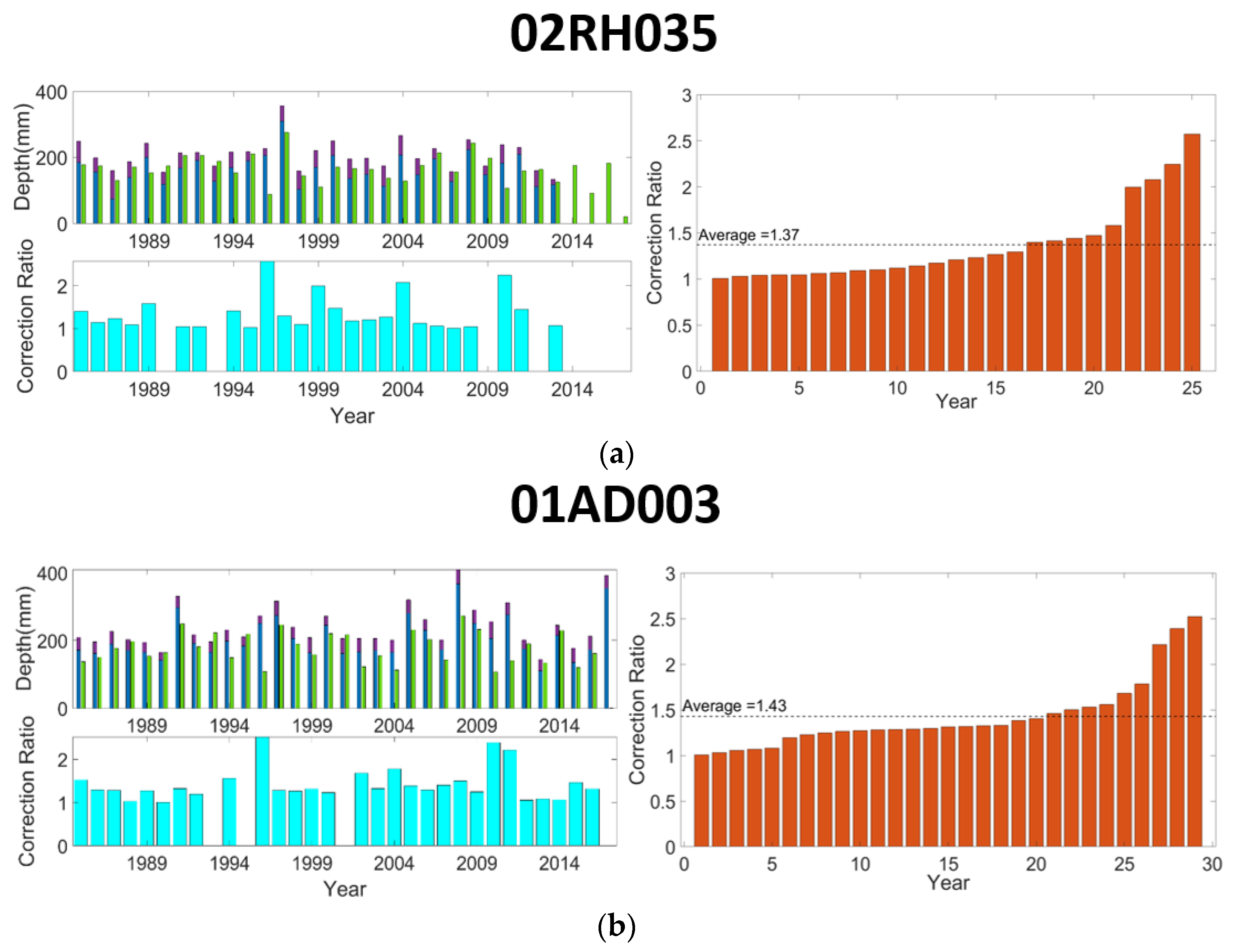
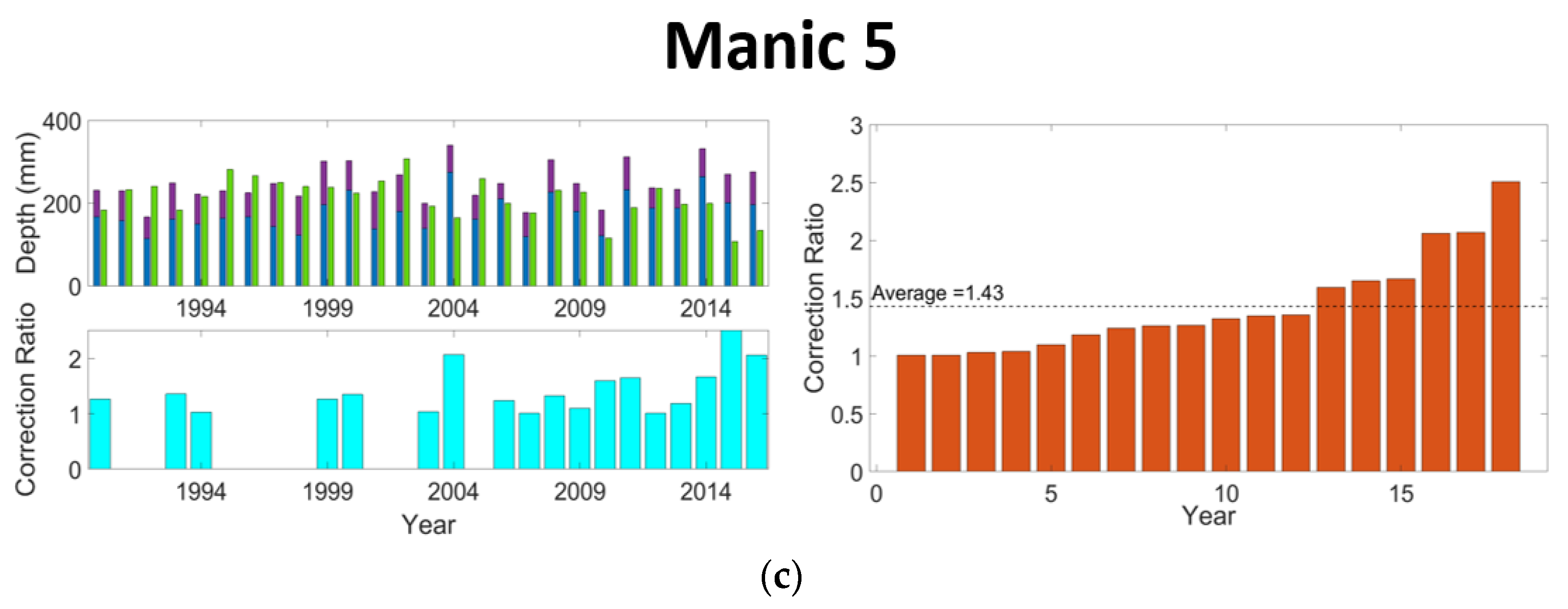
Correction factors (CF) values were computed for all watersheds and years under study according to Equation (5). This was done through estimation of the direct runoff DRH, calculated with Equation (3) by removal of the estimated baseflow from total runoff estimated from gauged stations. Direct runoff was also estimated from SWEmax data from GlobSnow, that is DRG, and considering precipitation and watershed infiltration occurring during the snowmelt period. Results are shown in Figure 5 and Table 3.
As expected, CF values of a given watershed vary from year-to-year in response to varying snowpack characteristics (e.g., stratigraphy, grain size), which are much simplified in the radiative transfer model (HUT) used to retrieve GlobSnow’s SWE estimates. Any important deviation from this snowpack representation will affect SWE estimation; for example, the presence of ice lenses in the snowpack may have a significant effect on microwave scattering and emission properties of the pack. This in turn may be wrongly interpreted as a snowpack with smaller SWE than reality, producing a larger CF value (CF > 1) (Equation (5)). Therefore, year-to-year variations in CF values can be seen as a consequence of varying hydrometeorological conditions leading to a heterogeneous snowpack, which are not adequately simulated by the HUT model used to estimate SWE. Saturation of the microwave signal as the snowpack gets thicker will also increase deviation of the estimated SWE compared to the ‘real’ SWE and, therefore, it is expected that large CF values will be obtained for years with thicker snowpack.
The average CF factor of the watersheds, as show in Table 3, has values ranging from 1.29 to 1.91. These results indicate that the range is rather small. The standard deviation for the study ranged from 0.29 to 0.53 with higher deviations coming from watersheds furthest south of the St. Lawrence, which may be an indication of difficulty in retrieving SWE data from the satellite microwave signal. A possible cause for such difficulty is the presence of complex snowpack stratigraphy, e.g., ice lenses, resulting from mid-winter rain-on-snow and freeze-thaw events, which are common in these regions. This is in contrast to watersheds located further north, where such meteorological events are less susceptible to occurs and therefore where snowpack is generally more homogeneous. Consequently, standard deviation of the retrieved CF factors is generally smaller.
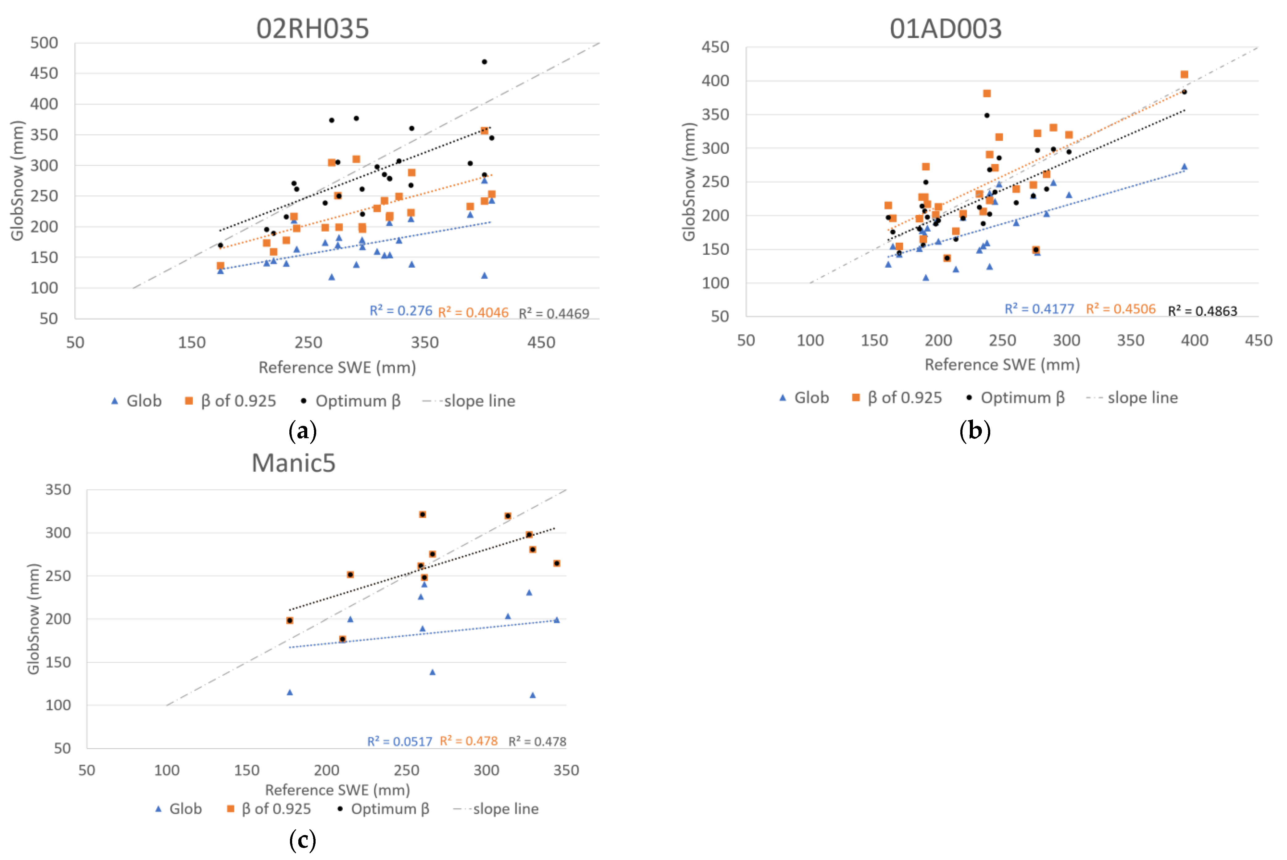
Figure 6 shows examples of scatterplots of available in situ maximum SWE data against the original and corrected GlobSnow products with the recommended baseflow separation factor β = 0.925 for the 02RH035, 01AD003, and Manic5 watersheds.
The limited in situ measurements affected the analysis; for example, the Manic5 watershed only had 11 years of in situ measurements over the 18 possible years. The figure confirms that the original GlobSnow product underestimates SWEmax; for example, the observed SWEmax values of the 02RH035 watershed vary between 170 and 450 mm but the corresponding GlobSnow values range from 120 to 270 mm. After correction, using the recommended β of 0.925, the range increases from 130 to 355 mm. Similar behavior are observed for all watersheds under study. Despite the bias being reduced, an underestimation remains.
Predominantly, the WSC approach increased the estimation of SWEmax, as summarized in Table 4. The WSC approach increased the range between minimal and maximal SWEmax values, and reduced the bias when compared to the referenced SWEmax. However, the degree of linear correlation between estimated and reference SWEmax values did not increase for all watersheds, nor did the RMSE systematically decrease (for example, see 02PL005). An increase of RMSE means that the WSC approach increased the dispersion of the corrected SWEmax values with relation to observed SWEmax. This is related to uncertainties along the modelling chain leading to the corrected SWEmax product. For example, a recommended value of the baseflow separation factor β is 0.925 for all watersheds, but studies have shown that β can differ depending on the watershed’s characteristics [18]. Higher/lower β values will decrease/increase baseflow and, therefore, directly affect the magnitude of direct runoff (DRH) and the magnitude of the corresponding correction factor (CF). The issue of model uncertainty is addressed later in this paper.
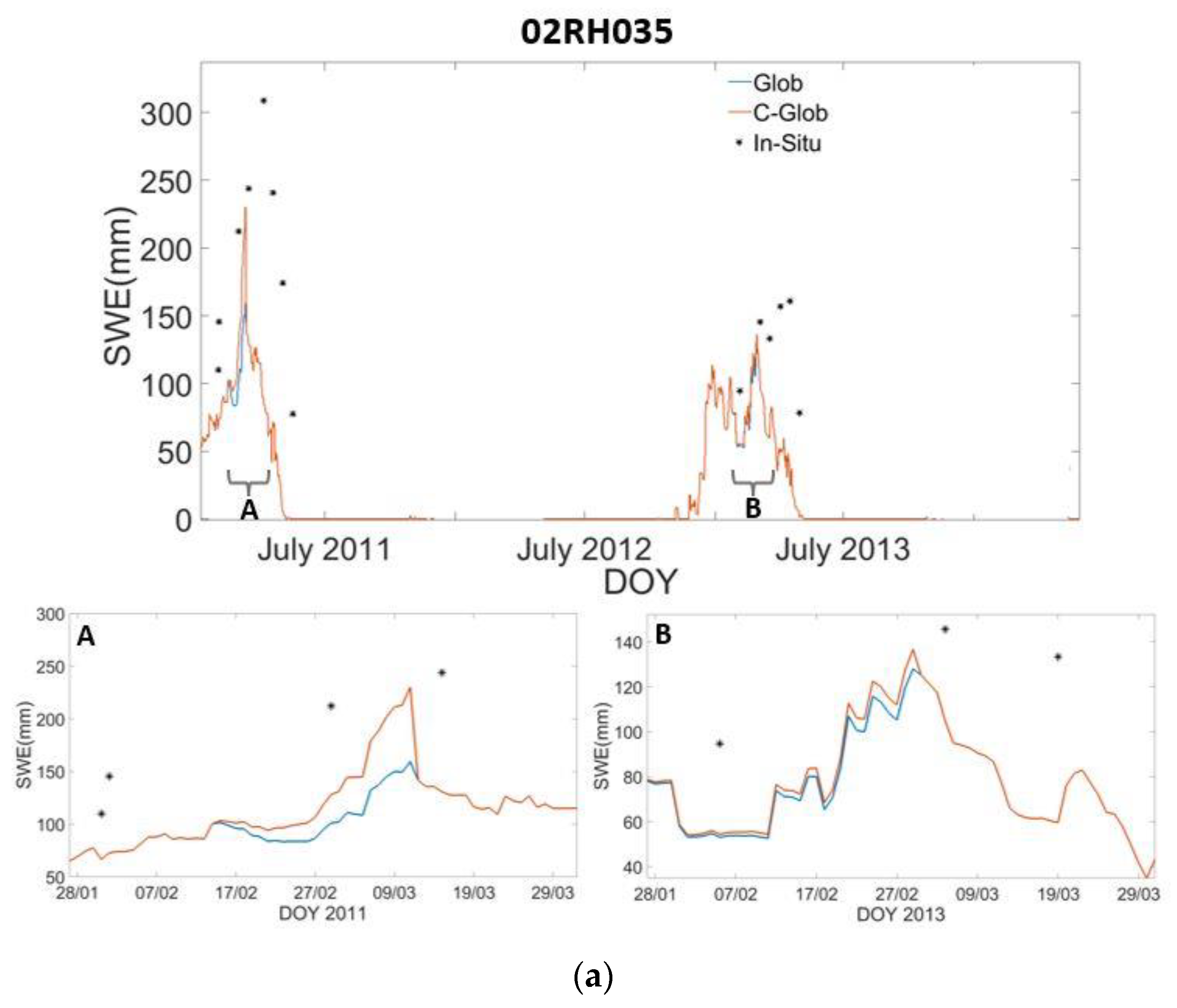
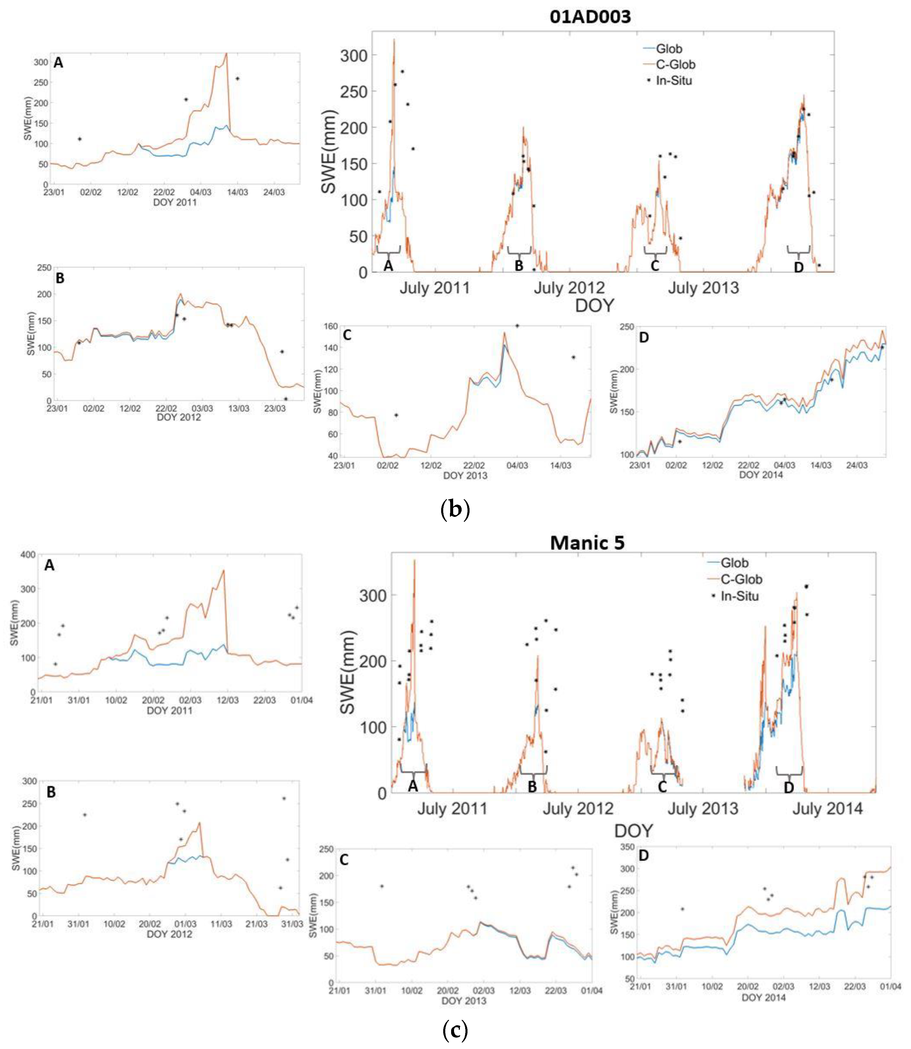
The time series of the corrected GlobSnow product and the original GlobSnow against in situ SWE is shown in Figure 7. Once the snowpack is developed, the corrected SWE estimation becomes greater than the original GlobSnow estimation and approaches the in situ SWE data. However, the corrected GlobSnow still underestimates SWE for some years and overestimates for others. Overestimation occurs in years that have gaps in the in situ SWE data around the time when GlobSnow estimates the snowpack to be at its peak.
4. Discussion
In this study, we proposed a hydrograph-based approach to correct the underestimation of SWE derived from remotely sensed passive microwave data (PM), specifically, the GlobSnow product. The chief advantage of our Watershed Scale Correction (WSC) approach is that it uses data that commonly already exists (i.e., flow at gauged stations and remotely sensed data) and that it does not require labour intensive and costly field measurements of SWE. This contrasts with more ‘classical’ approaches that consist of merging point SWE measurements to SWE maps derived from PM. Moreover, the WSC approach preserves GlobSnow’s physically based approach, but additionally incorporates a scaling factor derived from hydrological processes (i.e., direct runoff). While purely statistical approaches, such as spatial interpolation (e.g., simple approaches such as Thiessen polygons to more sophisticated methods such as kriging) between point SWE measurements have no physical basis. Additionally, the WSC approach allows for the correction of daily SWE products, such as GlobSnow, at the watershed scale, which SWE surveys cannot achieve. Therefore, the WSC approach reduces the need to have frequent field surveys to have greater temporal information on the state of watersheds. Therefore, the WSC approach adds value in the continued interest of presenting watershed state information on SWE during the snowpack accumulation period of winter. This in turn is valuable information for operational water resources managers to mitigate the threats of spring flood and also for optimal reservoir management for hydroelectric production.
Because PM typically underestimates SWE for deeper snowpacks [7], a number of physically based approaches have been proposed to correct the underestimation and have been successful. However, such approaches are complex to implement and are computer intensive when applied at the watershed scale. For example, LaRue et al. [14] implemented a chain of models to assimilate PM observations and obtained substantial bias reduction compared to original SWE simulations [14]. In their approach, they coupled the physically based Crocus snow model, driven by a global-scale atmospheric model, to the Dense Media Radiative Transfer-Multilayers (DMRT-ML) model to calibrate the snow stickiness parameter of DMRT-ML. They then assimilated AMSR-E TB observations in the calibrated DMRT-ML model to improve SWE estimations for 12 weather stations in northeastern Canada where continuous SWE measurements were available. Our WSC approach is comparatively simpler and can be applied to correct SWE at the watershed scale while retaining the physics of the algorithm used to convert TB into SWE.
Correction factor-based approaches were proposed in the literature and have been shown to provide more accurate SWE estimations. However, these approaches were developed to correct snowfall and not SWE directly. For example, Kang et al. [37] adjusted snowfall using a correction factor that was obtained by minimizing the difference between simulated SWE from a distributed hydrological model and observed SWE from PM. However, their approach is limited to shallow snowpacks because they assumed the reference SWE estimated from PM is unbiased, which does not hold true as the snowpack gets thicker. To our knowledge, no other study has presented an approach based on correcting SWE based on observed flow. Our WSC approach is relatively simple, requiring less complex modeling, and, therefore, is more user friendly.
4.1. Baseflow Separation as a Source of Uncertainty
As in any modelling approaches, the WSC has uncertainties in the modelling chain that affect results represented by the range of CF values obtained (see Figure 5 and Table 3). One uncertainty pertains to the HUT model’s simplification of the snowpacks complex structure (e.g., stratigraphy, crystallography) when converting the PM signal into SWE in the GlobSnow product (see results section for more details).
Another potentially important source of uncertainty relates to the baseflow separation technique used for estimating direct runoff. Nathan and McMahon [16] recommend that the baseflow filter coefficient (β) of the recursive filter approach should assigned the value of 0.925. However, Ref. [15] stipulate that the Hydrun toolbox used in our study (which is based on the digital recursive method) was not intended for cold regions winter analysis because it was originally developed by associating a runoff event to a rainfall input event. Therefore, it is likely that the volume of direct runoff estimated using this method will be misrepresented for watersheds where slower melt events occur. This limitation likely contributed to errors, however, future versions of the toolbox is expected to include more detailed characterizations of snowmelt processes [15].
Using the current iteration of the toolbox, this source of uncertainty can be reduced by optimizing the β factor for each watershed. To do so, indirect approaches are required because baseflow is seldom directly measured. Gan and Zuo [17] proposed to use a hydrological model to fit the β factor to match simulated baseflow; however, the resulting optimized β factor will be dependent of the structure of the hydrological model used to perform baseflow matching. In contrast, we optimized the β factor by minimizing the distance between GlobSnow’s SWEmax and observed SWEmax and, thus, our method is not model dependent. However, the drawback is that in situ SWEmax measurements are required, which negates the WSC approach’s prime advantage of not requiring in situ SWE measurements.
The optimization process is summarized in Table 5 that details the % bias of the corrected GlobSnow SWEmax relative the reference SWEmax for different baseflow β factors. The % bias for the recommended β value of 0.925 is shown in this table. With this β value the average bias was reduced to 18%, notably better than the Globsnow products 33.5% existing bias. While bold values are % bias which were minimized by adjusting β. Results indicate that using a single value for β fails to optimally correct for the underestimation of GlobSnow SWEmax values. Instead, β values vary from 0.800 to 0.995 for the 8 watersheds under analysis. Interestingly, the average β is 0.914, which is close to the 0.925 recommended value of [16]. Adjusted β values reduced the bias in the WSC approach as illustrated in Figure 6. Moreover, RMSE was reduced, and the degree of linear correlation overall increased, as shown in Table 6. Optimizing β values therefore contributed to reducing overall uncertainty.
We demonstrate that with watershed specific optimized β values, one can improve SWEmax estimation from GlobSnow. However, this is at the expense of requiring in situ SWEmax measurements. One way to avoid requiring in situ SWE, would be to develop a relationship between β and watershed physiographic and/or hydroclimatic characteristics and apply such relationship to watersheds where SWE is not measured.
This was attempted here, although a small number of watersheds were analysed which limits the robustness of our findings. Therefore, more watersheds need to be incorporated into such analysis to confirm the reported relationships below.
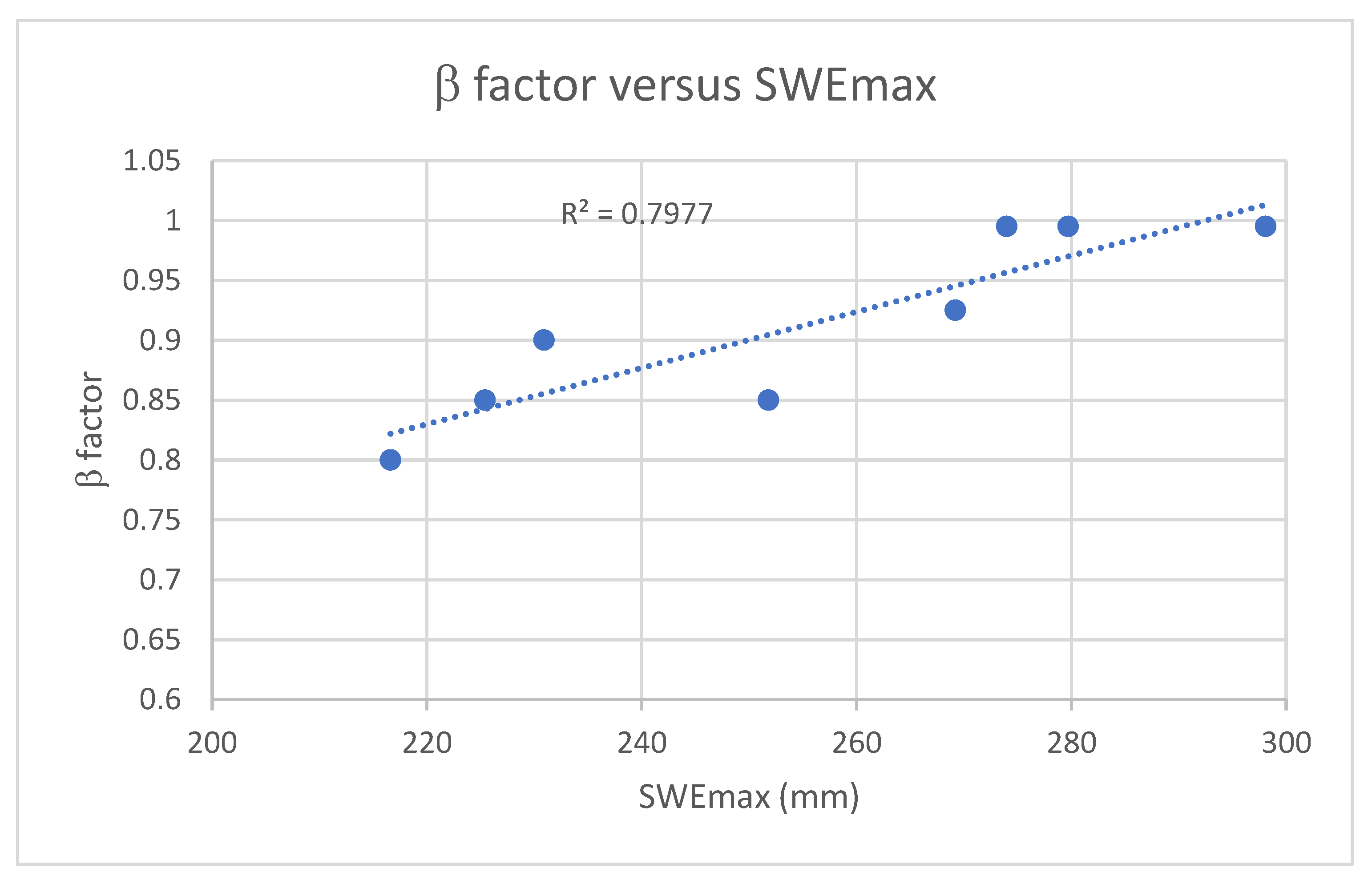
As a first attempt, we investigated the relationship between β and in situ SWEmax, see Figure 8. We found a strong linear relationship, with a R2 value of 0.798; deeper snowpacks, which have larger volumes of spring melt runoff, had larger β values. Recall that larger β value is associated with a lower contribution of baseflow to total runoff, while a lower β value means that the baseflow contribution is more significant to total runoff. This behaviour aligns with the nature of infiltration in northern watersheds, which is restricted and, sometimes almost completely limited, by a layer of frozen ground. Therefore, saturation overland flows occur as the soil above the frozen soil layer becomes saturated and any additional snowmelt (and rainfall) causes runoff.
Our second attempt was to unravel possible relationships between β values and watershed physiographic characteristics (i.e., geology/pedology) as this influences baseflow. Indeed, baseflow—which is not to confused with groundwater flow—is the proportion of river runoff from stored sources such as soils, surficial deposits and permeable rocks. We observed that the watersheds located in the Appalachian region (0PL005, 02PG022, 01AD003 and 01010000) had lower β values, ranging from 0.800 to 0.900, whereas the watersheds located in the Canadian Shield (0RH035, 02PA007 and 02NE011) had higher value of 0.995. These two regions are characterized by different geological and pedological characteristics that likely effect baseflow. The Canadian Shield is generally associated with thin soils and the occurrence of granitic, gneiss, and volcanic bedrock where the capacity to store water is small. For example, at study sites characterized as Canadian Shield in Ontario, Refs. [38,39] found that water storage capacity to be only 6 mm and 8 mm, respectively. In contrast, the Appalachian region is mostly characterized by sedimentary bedrock covered with fine-to-deep glacial deposits where flow through fractured sediment rock and superficial deposits are more likely to occur. We argue that these different geologic and pedologic regimes of these regions may explain differences observed in the β values of watersheds, where lower/higher β values are associated with higher/lower baseflow contribution to total runoff. Additional analyses using more watersheds are needed to validate this hypothesis.
4.2. Other Sources of Uncertainty
In addition to snowpack structure and baseflow separation techniques, other sources of uncertainties in the WSC approach (see Equation (5)) include precipitation during the melt period (P), modelling infiltration into frozen ground (I), and total runoff as measured at the gaging station (ROtotal).
The accuracy of total precipitation (P) during the melt period is source dependent. Here we used the ERA5 daily precipitation that, according to Xiong et al. [40], shows good accuracy especially for the winter in our study region. Although, Crossett et al. [41] indicate that ERA5 underestimates precipitation along the Atlantic coast but overestimates precipitation inland compared to in situ observational weather stations. Despite that, ERA5 and similar products are particularly well suited for regions where weather stations are scarce and for larger watersheds, such as Manic5. However, for smaller watersheds and where weather station density is high, such as the study sites located in the Appalachian region, it may be preferable to use in situ observations. In this study, P was estimated from the ERA5 global reanalysis and therefore contains its uncertainties. This may affect the accuracy of the CF derived, impacting the corresponding corrected GlobSnow product.
Frozen ground infiltration was estimated using Gray’s model (Equation (8)), which requires average near-surface (40 cm) soil saturation (SI) and temperature (TI) that were retrieved from the ERA5 reanalysis product. The ERA5 reanalysis product uses soil texture information to simulate SI and TI, where soil texture is categorized using the seven soil types derived from the root zone data of the FAO/UNESCO Digital Soil Map of the World [42]. However, this coarse representation of the true soil types inevitably introduced errors in SI and TI, and incorporating these products into the limited infiltration equation may have enhanced the bias associated with the algorithm and led to additional errors. Future works will benefit from the addition of in situ soil data that more accurately represents infiltration.
The opportunity time (t0) is another variable affecting estimation of the infiltration into frozen ground, which is calculated according to Equation (9). For simplicity, we determined t0 from the ERA5 SWEmax and snow cover extent (SCE) product. Although the time at which SWEmax occurs is rather straightforward to obtain, the time at which snow cover completely disappears is more difficult to retrieve because of the relatively low spatial resolution of the product. One way to improve future estimations of t0 would be to use high spatial resolution snow cover data sets when available.
Given that t0 corresponds to the duration of the snowmelt period, which was used to calculate the amount of precipitation (P), any error in estimating t0 will also have repercussions on the estimation of P. Ideally, one should use the time during which surface runoff is occurring to calculate P across this period. This could be retrieved from a baseflow separation analysis; however, in our work, given the uncertainty at estimating the β filter parameter, we decided to approximate the runoff duration time as the duration of the snowmelt period. For small to medium size watersheds, this will have a minimal impact as the time of concentration is in the order of hours to a few days. However, in larger watersheds such as Manic5, the time of concentration will be several days and, therefore, will potentially impact the estimation of total precipitation during the opportunity time.
A rating curve is used for converting surface water elevation into river discharge. The curve is a relationship between water levels and discharges at a specific cross-section of the stream or the river and is established using gauged discharges and water levels. Rating curves can lead to significant errors. These errors can arise from a suite of operational factors (e.g., the number of sampling points and location of gauged section) and the uncertainty in discharge measurements might be as high as 20% of the observed value [43]. Furthermore, since discharge measurements are often impracticable during high floods, extrapolation errors are generally introduced. Additionally, rating curves may provide poor estimates of river discharge under ice conditions, as the river cross-section is constricted and produces higher river stage compared to ice-free periods. Any increase/decrease of river flow will directly impact CF values, see Equation (5). For example, assuming in a hypothetical watershed a ±10% uncertainty on river discharge, where P = 20 mm, I = 0, SWEmax = 250 mm, total runoff = 350 mm and baseflow = 30 mm would result in CF ranging between 1.20 and 1.52.
4.3. The SWC Approach as Part of an Ensemble Flow Forecast System
Although the above uncertainties result in a range of watershed-scale CF values, we argue that this is an appealing feature when applying the WSC approach to probabilistic flow forecasts. An ensemble of corrected GlobSnow SWE values can be used to set initial conditions of a hydrological model for generating ensemble flow forecasts. As mentioned above, a 5-km GlobSnow SWE product is available 12 h after global satellite data has been acquired (data available in the Copernicus site). Therefore, the raw SWE product can be used to generate near real time corrected products. This is particularly useful to agencies concerned by spring flow forecasts, e.g., hydropower companies and river forecast centers, as forecasting flow scenarios becomes possible with estimates of corrected SWE at near real time, along with forecasted temperature and precipitation information.
While the WSC approach strictly applies to correct SWEmax estimates from PM data (here GlobSnow), in the context of operational flood forecasting, one needs to correct SWE at any time a flow forecast is required. This requires having CF varying over time during snowpack build-up. Here, we proposed a simple linear relationship between CF and SWE from GlobSnow, see Figure 2, with a lower bound of CF = 1 and the upper value calculated according to equation 5. Whether or not a linear relationship between CF and SWE truly reflects the expected evolution of CF across the snowpack buildup remains to be validated by comparing resulting SWE values against in situ SWE(t) measurements.
In a probabilistic forecast world, the WSC approach produces an ensemble of SWEmax values. Combining the ensemble with the CF(SWE) relationship (Figure 2), results in an ensemble of corrected SWE values each time a forecast is issued. Therefore, the corresponding probability distribution of corrected SWE at a given time only depends the corrected SWEmax distribution and on CF-SWE relationship. Beneficially, no exogeneous information (e.g., observed SWE at the time a forecast is issued) is involved in defining the distribution. With better knowledge on the trajectory of SWE as the snowpack gradually accumulates (e.g., whether a thick or a thin snowpack is anticipated at the onset of the spring melt), one may update the probability distribution of the corrected SWEmax. In other words, having the prior distribution of SWEmax, one would obtain the posterior distribution of SWEmax with knowledge of SWE at time t using a statistical inference method such as Bayesian inference:
where is the posterior probability of H given E, is the prior probability of H and is the probability of observing E given H. In this equation, H = SWEmax and E = SWE at a given time t. , , and can all be obtained from historical observations of SWE, including SWEmax.
Alternatively, the most likely SWEmax value in a given year could be computed/updated each time new exogenous information affecting SWEmax becomes available. This would require leveraging historical data to develop a statistical model between SWEmax and exogenous variables at time t, such as the current SWE value. Using this approach, the most likely SWEmax value computed at the time a forecast is issued would be used to correct the current SWE value using the CF-SWE relationship (Figure 2).
4.4. Validation of the WSC Approach: An Issue of Scale Mismatch
In this study, we describe a novel approach for correcting a remote sensing derived SWE product that avoids using in situ SWE measurements. However, as with the development of any quantitative remote sensing algorithm, we are limited in our ability to effectively validate the approach due to the severe spatial scale discrepancy between the data source used as the benchmark (i.e., in situ SWE measurements), and model product (i.e., corrected GlobSnow SWE). As pointed out by Wu [44] (p. 1769), ‘Scale effects constrain the accuracy of retrieval and limit the development of remote sensing applications’. Therefore, it is important to match the reference SWE and the corrected SWE product to a common scale, here the watershed scale, for proper validation. The simplest upscaling approach is the arithmetic mean (a member of the Area-Weighted Methods family), which was used in this work.
In situ SWE sites are carefully selected to be representative surrounding areas by avoiding local effects on SWE values; for example, sites where wind effects are significant (resulting in either underestimating or overestimating the ‘true’ SWE) are avoided. Despite such cautions, accurate local SWE measurements may not be representative of the watershed scale SWE if the number of measurement sites is small, as is the case for this study. Benchmark SWE values were obtained from only one or two in situ SWE measurements for all watersheds under study, except for the Manic 5 watershed, where 5 stations were used (locations of in situ measurements illustrated in Figure 2). Therefore, the low number of in situ stations used to obtain the reference SWE may explain situations where poor fits between the reference and the corrected SWE were obtained, in addition to the various sources of uncertainty discussed above. For example, watershed 01AD003 in 2010 was found to have a poor fit, where the corrected GlobSnow SWEmax differed from the reference SWEmax by 140 mm, resulting in a 60% deviation from the reference (note that this was obtained using β = 0.925). An improved data archive or SWEmax would not only allow for better validation of the WSC approach but would also help in better defining relationships between the optimal β factor and SWEmax discussed above. Datasets such as SNODAS [45] and CanSWE [46] may be considered for setting the benchmark.
5. Conclusions
In this study, we demonstrate the usefulness of integrating additional physical hydrological processes, specifically direct runoff, in the bias correction of GlobSnow, a global SWE database derived from space-borne passive microwave sensors. Unlike other physically based approaches that are more computer intensive and complex to implement, the WSC approach can correct SWE at the watershed scale while preserving the physics of the temperature brightness algorithm used in SWE conversion.
As with all modeling approaches, there are issues relating to uncertainties with the WSC approach; of those, the most critical to the output was the baseflow separation technique used in estimating direct runoff. While the recommended value of the baseflow filter coefficient (β = 0.925) for the recursive filter approach, overall reduced bias for all studied watersheds, we found that optimizing the β value for watersheds better corrected for the underestimation of GlobSnow SWEmax values reducing overall uncertainty. We found that the deeper the snowpack the larger the corresponding β value, which is in line with the limited nature of infiltration in northern watersheds. Incorporating in situ soil data will reduce uncertainty associated with using the Gray’s model to determine infiltrability. Additional uncertainty comes from the rating curve as it may provide poor estimates of river discharge under icy conditions as CF is sensitive to any increase or decrease in the river flow.
Despite these uncertainties, the WSC approach can be used for probabilistic flow forecasts. GlobSnow produces a near real time 5-km SWE product and an ensemble of corrected GlobSnow SWE produced using the WSC approach could be used to initialize conditions of a hydrological model. This application may be particularly useful to water management organizations concerned about spring flows.
To conclude, our WSC approach performed acceptably, increasing the accuracy of SWEmax estimates when compared to in situ measurements for the studied watersheds. However, due to a scale discrepancy between the data used as benchmark and model product, and the representability of the local measurements to be used as a representative for the watershed, there were situations of poor fit. An improved benchmark would allow for better validating the WSC approach. Future studies will be dedicated to improving the benchmark and other assumptions made in evaluation of the approach.
Author Contributions
C.W. and R.L. contributed to the conception and design. C.W. performed Data analysis; C.W. prepared the original manuscript draft and did edits; R.L. reviewed and edited the manuscript and supervised the study. All authors have read and agreed to the published version of the manuscript.
Funding
This research was funded as part of the Canadian Natural Science and Engineering Research Council (NSERC) Industrial Research Chair on the Application of Hydrometeorological Data from Satellite Images to Improve Hydrological Forecasting. Financial support came from the following organizations: Hydro-Quebec, Brookfield and the City of Sherbrooke.
Data Availability Statement
Observed SWE data was obtained through private communications and is not available for sharing.
Conflicts of Interest
The authors declare no conflict of interest.
References
- Buttle, J.M.; Allen, D.M.; Caissie, D.; Davison, B.; Peters, D.L.; Pomeroy, J.W.; Simonovic, S.; St-Hilaire, A.; Whitfield, P.H. Flood Processes in Canada: Regional and Special Aspects. Can. Water Resour. J. 2016, 41, 7–30. [Google Scholar] [CrossRef]
- Foulon, É.; Rousseau, A.N.; Gagnon, P. Development of a Methodology to Assess Future Trends in Low Flows at the Watershed Scale Using Solely Climate Data. J. Hydrol. 2018, 557, 774–790. [Google Scholar] [CrossRef] [Green Version]
- Neumann, N.N.; Derkens, C.; Smith, C.; Goodison, B. Characterizing Local Scale Snow Cover Using Point Measurements during the Winter Season. Atmosphere-Ocean 2006, 44, 257–269. [Google Scholar] [CrossRef]
- De Gregorio, L.; Günther, D.; Callegari, M.; Strasser, U.; Zebisch, M.; Bruzzone, L.; Notarnicola, C. Improving SWE Estimation by Fusion of Snow Models with Topographic and Remotely Sensed Data. Remote Sens. 2019, 11, 2033. [Google Scholar] [CrossRef] [Green Version]
- Vuyovich, C.; Jacobs, J.M. Remote Sensing of Environment Snowpack and Runoff Generation Using AMSR-E Passive Microwave Observations in the Upper Helmand Watershed, Afghanistan. Remote Sens. Environ. 2011, 115, 3313–3321. [Google Scholar] [CrossRef]
- Tiuri, M.E.; Sihvola, A.H.; Nyfors, E.G.; Hallikaiken, M.T. The Complex Dielectric Constant of Snow at Microwave Frequencies. IEEE J. Ocean. Eng. 1984, 9, 377–382. [Google Scholar] [CrossRef]
- Larue, F.; Royer, A.; De Sève, D.; Langlois, A.; Roy, A.; Brucker, L. Validation of GlobSnow-2 Snow Water Equivalent over Eastern Canada. Remote Sens. Environ. 2017, 194, 264–277. [Google Scholar] [CrossRef] [Green Version]
- Derksen, C.; Walker, A.E.; Goodison, B.E.; Strapp, J.W. Integrating In Situ and Multiscale Passive Microwave Data for Estimation of Subgrid Scale Snow Water Equivalent Distribution and Variability. IEEE Trans. Geosci. Remote Sens. 2005, 43, 960–972. [Google Scholar] [CrossRef]
- Koenig, L.S.; Forster, R.R. Evaluation of Passive Microwave Snow Water Equivalent Algorithms in the Depth Hoar-Dominated Snowpack of the Kuparuk River Watershed, Alaska, USA. Remote Sens. Environ. 2004, 93, 511–527. [Google Scholar] [CrossRef]
- Pulliainen, J. Mapping of Snow Water Equivalent and Snow Depth in Boreal and Sub-Arctic Zones by Assimilating Space-Borne Microwave Radiometer Data and Ground-Based Observations. Remote Sens. Environ. 2006, 101, 257–269. [Google Scholar] [CrossRef]
- Luojus, K.; Pulliainen, J.; Takala, M.; Lemmetyinen, J.; Mortimer, C.; Derksen, C.; Mudryk, L.; Moisander, M.; Hiltunen, M.; Smolander, T.; et al. GlobSnow v3.0 Northern Hemisphere Snow Water Equivalent Dataset. Sci. Data 2021, 8, 163. [Google Scholar] [CrossRef]
- Takala, M.; Luojus, K.; Pulliainen, J.; Derksen, C.; Lemmetyinen, J.; Kärnä, J.; Koskinen, J.; Bojkov, B. Remote Sensing of Environment Estimating Northern Hemisphere Snow Water Equivalent for Climate Research through Assimilation of Space-Borne Radiometer Data and Ground-Based Measurements. Remote Sens. Environ. 2011, 115, 3517–3529. [Google Scholar] [CrossRef]
- Pulliainen, J.; Hallikainen, M. Retrieval of Regional Snow Water Equivalent from Space-Borne Passive Microwave Observations. Remote Sens. Environ. 2001, 75, 76–85. [Google Scholar] [CrossRef]
- Larue, F.; Royer, A.; De Sève, D.; Roy, A.; Picard, G.; Vionnet, V.; Cosme, E. Simulation and Assimilation of Passive Microwave Data Using a Snowpack Model Coupled to a Calibrated Radiative Transfer Model Over Northeastern Canada. Water Resour. Res. 2018, 54, 4823–4848. [Google Scholar] [CrossRef]
- Tang, W.; Carey, S.K. HydRun: A MATLAB Toolbox for Rainfall—Runoff Analysis. Hydrol. Process. 2017, 31, 2670–2682. [Google Scholar] [CrossRef]
- Nathan, R.J.; McMahon, T.A. Evaluation of Automated Techniques for Base Flow and Recession Analyses. Water Resour. Res. 1990, 26, 1465–1473. [Google Scholar] [CrossRef]
- Gan, R.; Zuo, Q. Assessing the Digital Filter Method for Base Flow Estimation in Glacier Melt Dominated Basins. Hydrol. Process. 2016, 30, 1367–1375. [Google Scholar] [CrossRef]
- Mau, D.P.; Winter, T.C. Estimating Ground-Water Recharge from Streamflow Records. Ground Water 1997, 35, 291–304. [Google Scholar] [CrossRef]
- Hammond, J.C.; Kampf, S.K. Subannual Streamflow Responses to Rainfall and Snowmelt Inputs in Snow-Dominated Watersheds of the Western United States. Water Resour. Res. 2020, 56, e2019WR026132. [Google Scholar] [CrossRef]
- Voutchkova, D.D.; Miller, S.N.; Gerow, K.G. Parameter Sensitivity of Automated Baseflow Separation for Snowmelt-Dominated Watersheds and New Filtering Procedure for Determining End of Snowmelt Period. Hydrol. Process. 2018, 33, 876–888. [Google Scholar] [CrossRef]
- Fan, Y.; Chen, Y.; Liu, Y.; Li, W. Variation of Baseflows in the Headstreams of the Tarim River Basin during 1960–2007. J. Hydrol. 2013, 487, 98–108. [Google Scholar] [CrossRef]
- Gray, D.M.; Toth, B.; Zhao, L.; Pomeroy, J.W.; Granger, R.J. Estimating Areal Snowmelt Infiltration into Frozen Soils. Hydrol. Process. 2001, 15, 3095–3111. [Google Scholar] [CrossRef]
- Nicholaichuk, W.; Gray, D.M. Snow Trapping and Moisture Infiltration Enhancement. In Proceedings of the 5th Annual Western Provinces Conference Rationalization of Soil and Water Research and Management, Calgary, AB, Canada, 18–20 November 1986. [Google Scholar]
- Zhao, L.; Gray, D.M. Estimating Snowmelt Infiltration into Frozen Soils. Hydrol. Process. 1999, 1842, 1827–1842. [Google Scholar] [CrossRef]
- De Sève, D.; Évora, N.D.; Tapsoba, D. Comparison of Three Algorithms for Estimating Snow Water Equivalent (SWE) over the La Grande River Watershed Using SSM/I Data in the Context of Hydro-Qúbec’s Hydraulic Power Management. In Proceedings of the IEEE International Geoscience and Remote Sensing Symposium, Barcelona, Spain, 23–27 July 2007; pp. 4257–4260. [Google Scholar] [CrossRef]
- Langlois, A.; Royer, A.; Derksen, C.; Montpetit, B.; Dupont, F.; Gota, K. Coupling the Snow Thermodynamic Model SNOWPACK with the Microwave Emission Model of Layered Snowpacks for Subarctic and Arctic Snow Water Equivalent Retrievals. Water Resour. Res. 2012, 48, 1–14. [Google Scholar] [CrossRef] [Green Version]
- Luojus, K.A.R.I.L.; Ulliainen, J.O.P.; Akala, M.A.T.; Emmetyinen, J.U.H.A.L.; Angwa, M.W.K.; Molander, T.U.S. Algorithm Theoretical Basis Document—SWE-Algorithm. 2013. Available online: https://www.globsnow.info/docs/GS2_SWE_ATBD.pdf (accessed on 6 October 2022).
- Chen, J.; Brissette, F.P.; Chaumont, D.; Braun, M. Performance and Uncertainty Evaluation of Empirical Downscaling Methods in Quantifying the Climate Change Impacts on Hydrology over Two North American River Basins. J. Hydrol. 2013, 479, 200–214. [Google Scholar] [CrossRef]
- Badreddine, S.F.; Goïta, K.; Vachon, F.; De Sherbrooke, U. Comparison of Quebec Snow Grid Data and GlobSnow Products over the La Grande and Manicouagan Watersheds in Canda from 2006 to 2010. In Proceedings of the IGARSS 2018-2018 IEEE International Geoscience and Remote Sensing Symposium, Valencia, Spain, 22–27 July 2018; pp. 5216–5219. [Google Scholar] [CrossRef]
- Chen, J.; Brissette, F.P.; Leconte, R. Uncertainty of Downscaling Method in Quantifying the Impact of Climate Change on Hydrology. J. Hydrol. 2011, 401, 190–202. [Google Scholar] [CrossRef]
- Arsenault, R.; Brissette, F.; Martel, J.; Troin, M.; Lévesque, G.; Davidson-chaput, J.; Gonzalez, M.C.; Ameli, A.; Poulin, A. A Comprehensive, Multisource Database for Hydrometeorological Modeling of 14, 425 North American Watersheds. Sci. Data 2020, 7, 243. [Google Scholar] [CrossRef] [PubMed]
- Takala, M.; Ikonen, J.; Luojus, K.; Lemmetyinen, J.; Metsamaki, S.; Cohen, J.; Arslan, A.N.; Pulliainen, J. New Snow Water Equivalent Processing System with Improved Resolution over Europe and Its Applications in Hydrology. IEEE J. Sel. Top. Appl. Earth Obs. Remote Sens. 2016, 10, 428–436. [Google Scholar] [CrossRef]
- Luojus, K.; Lemmetyinen, J.; Pulliainen, J.; Takala, M.; Moisander, M.; Cohen, J.; Ikonen, J. Copernicus Global Land Operations “Cryosphere and Water” Algorithm Theoretical Basis Document. 2017. Available online: https://land.copernicus.eu/global/sites/cgls.vito.be/files/products/CGLOPS2_ATBD_SWE-NH-5km-V1_I1.01.pdf (accessed on 6 October 2022).
- Tang, W.; Qin, J.; Yang, K.; Zhu, F.; Zhou, X. Does ERA5 Outperform Satellite Products in Estimating Atmospheric Downward Longwave Radiation at the Surface? Atmos. Res. 2021, 252, 105453. [Google Scholar] [CrossRef]
- Muñoz-sabater, J.; Dutra, E.; Agustí-panareda, A.; Albergel, C.; Hersbach, H.; Martens, B.; Miralles, D.G.; Piles, M.; Rodríguez-fernández, N.J. ERA5-Land: A State-of-the-Art Global Reanalysis Dataset for Land Applications. Earth Syst. Sci. Data 2021, 13, 4349–4383. [Google Scholar] [CrossRef]
- Hersbach, H.; Bell, B.; Berrisford, P.; Hirahara, S.; Horányi, A.; Nicolas, J.; Peubey, C.; Radu, R.; Bonavita, M.; Dee, D.; et al. The ERA5 Global Reanalysis. Q. J. R. Meteorol. Soc. 2020, 146, 1999–2049. [Google Scholar] [CrossRef]
- Kang, D.; Lee, K.; Kim, E.J. Improving Cold-Region Streamflow Estimation by Winter Precipitation Adjustment Using Passive Microwave Snow Remote Sensing Datasets. Environ. Res. Lett. 2021, 16, 044055. [Google Scholar] [CrossRef]
- Allan, C.J.; Roulet, N.T. Runoff Generation in Zero-order Precambrian Shield Catchments: The Stormflow Response of a Heterogeneous Landscape. Hydrol. Process. 1994, 8, 369–388. [Google Scholar] [CrossRef]
- Peters, D.L.; Buttle, J.M.; Taylor, C.H.; LaZerte, B.D. Runoff Production in a Forested, Shallow Soil, Canadian Shield Basin. Water Resour. Res. 1995, 31, 1291–1304. [Google Scholar] [CrossRef]
- Xiong, W.; Tang, G.; Wang, T.; Ma, Z.; Wan, W. Partitioning on the Global Scale. Water 2022, 14, 1122. [Google Scholar] [CrossRef]
- Crossett, C.C.; Betts, A.K.; Dupigny-Giroux, L.A.L.; Bomblies, A. Evaluation of Daily Precipitation from the Era5 Global Reanalysis against Ghcn Observations in the Northeastern United States. Climate 2020, 8, 148. [Google Scholar] [CrossRef]
- Hartemink, A.E.; Krasilnikov, P.; Bockheim, J.G. Soil Map of the World. Nature 1957, 179, 1168. [Google Scholar] [CrossRef]
- Domeneghetti, A.; Castellarin, A.; Brath, A. Assessing Rating-Curve Uncertainty and Its Effects on Hydraulic Model Calibration. Hydrol. Earth Syst. Sci. 2012, 16, 1191–1202. [Google Scholar] [CrossRef]
- Wu, H.; Li, Z.L. Scale Issues in Remote Sensing: A Review on Analysis, Processing and Modeling. Sensors 2009, 9, 1768–1793. [Google Scholar] [CrossRef]
- Barrett, A.P. National Operational Hydrologic Remote Sensing Center Snow Data Assimilation System (SNODAS) Products at NSIDC; National Snow and Ice Data Center: Boulder, CO, USA, 2003. [Google Scholar]
- Vionnet, V.; Mortimer, C.; Brady, M.; Arnal, L.; Brown, R. Canadian Historical Snow Water Equivalent Dataset (CanSWE, 1928–2020). Earth Syst. Sci. Data 2021, 13, 4603–4619. [Google Scholar] [CrossRef]
Figure 1.
Overall methodology of the WSC approach developed for computing CF.

Figure 2.
Schematic of linear relationship between SWE and correction factors.

Figure 3.
Study watersheds with location of SWE surveys (circular points). Watershed IDs taken from the HYSET database [31].
Figure 3.
Study watersheds with location of SWE surveys (circular points). Watershed IDs taken from the HYSET database [31].

Figure 4.
Watershed scale SWE retrieved from GlobSnow: (a) 02RH035 (Rivière des Écorces), (b) 01AD003 (St-Francis), and (c) Manic 5 watersheds. Blue line: average SWE; black line: maximum SWE.
Figure 4.
Watershed scale SWE retrieved from GlobSnow: (a) 02RH035 (Rivière des Écorces), (b) 01AD003 (St-Francis), and (c) Manic 5 watersheds. Blue line: average SWE; black line: maximum SWE.


Figure 5.
CF values of Manic5 (a), 02RH035 (b) an 01AD003 (c) watersheds. For each watershed, upper left graph shows the direct runoff hydrograph (DRH) in blue, watershed infiltration (I) in purple, and maximum snow water equivalent from GlobSnow () in green. Lower left graph shows the resulting CF values. Values lower than 1 are discarded. The graph to the right shows the sorted CF values ranked from lowest to largest. The average CF value is shown as the dotted line. In this figure, baseflow was estimated using β = 0.925.


Figure 6.
Scatter plots of in situ SWEmax data against the original and corrected GlobSnow products for (a) 02RH035, (b) 01AD003, and (c) Manic5 watersheds. Corrected GlobSnow with recommended baseflow separation factor β = 0.925 and with optimal β value are shown. The dashed line represents the 1:1 line.

Figure 7.
Temporal evolution of SWE for Glob (blue), C-Glob (orange) and in situ (black) data for watersheds (a) 02RH035, (b) 01AD003, and (c) Manic 5. Sub figures (A–D) represent specific years as indicated on the main plot. Note that no corrections are applied once SWEmax is reached because the WSC approach only applies during snowpack build-up. The Glob, C-Glob, and in situ data are averaged watershed measurements.


Figure 8.
Scatterplot of the optimum β versus in situ SWE max.


Table 1.
Physiographic and hydrometeorological data of the watersheds under study.
| Long Term Averaged Measured Values | |||||
|---|---|---|---|---|---|
| Watershed ID | Station Name | Data Period | Area (km2) | SWEmax (mm) | Peak Flow (m3/s) |
| 02RH035 | aux Écorces River at highway-bridge 169 | 1985–2013 | 1110 | 298 | 166 |
| 01AD003 | St. Francis River at outlet of Glasier lake | 1985–2016 | 1359 | 231 | 200 |
| Manic5 | Manicouagan 5 | 2006–2016 | 24,698 | 269 | 2018 |
| 01010000 | St. John River at Ninemile Bridge | 1985–2016 | 3473 | 225 | 690 |
| 02NE011 | Croche River downstream of Changy Brook | 1985–2013 | 1570 | 274 | 190 |
| 02PA007 | Batiscan River downstream of des Envies River | 1985–2013 | 4480 | 280 | 551 |
| 02PL005 | Bécancour River upstream Palmer River | 1985–2013 | 919 | 217 | 214 |
| 02PG022 | Ouelle River near St. Gabriel de Kamouraska | 1986–2013 | 795 | 252 | 207 |
Table 2.
GlobSnow and in situ seasonal maximum SWEmax data.
| Watershed ID | Data Period | Average SWEmax | |
|---|---|---|---|
| GlobSnow Product | In Situ Measurements | ||
| 02RH035 | 1985–2013 | 171 | 298 |
| 01AD003 | 1985–2016 | 178 | 231 |
| Manic5 | 2006–2016 | 185 | 269 |
| 01010000 | 1985–2016 | 162 | 225 |
| 02NE011 | 1997–2013 | 158 | 274 |
| 02PA007 | 1985–2013 | 162 | 279 |
| 02PL005 | 1985–2013 | 151 | 216 |
| 02PG022 | 1985–2013 | 181 | 252 |
Table 3.
Computed CF values for all watersheds under study.
| Watershed ID | Area | GlobSnow Average SWEmax (mm) | CF | |||
|---|---|---|---|---|---|---|
| Average | Std Dev | Min | Max | |||
| 02RH035 | 1110 | 171 | 1.37 | 0.43 | 1.01 | 2.57 |
| 01AD003 | 1359 | 178 | 1.43 | 0.37 | 1.01 | 2.52 |
| Manic5 | 24,698 | 185 | 1.43 | 0.41 | 1.01 | 2.51 |
| 01010000 | 3473 | 162 | 1.78 | 0.53 | 1.10 | 3.47 |
| 02NE011 | 1570 | 158 | 1.29 | 0.29 | 1.02 | 2.27 |
| 02PA007 | 4480 | 162 | 1.36 | 0.33 | 1.01 | 2.66 |
| 02PL005 | 919 | 151 | 1.91 | 0.52 | 1.20 | 4.08 |
| 02PG022 | 795 | 181 | 1.74 | 0.40 | 1.15 | 2.77 |
Table 4.
Statistical summary of the original (Glob) and corrected (C-Glob) SWEmax. A negative bias means that GlobSnow and corrected GlobSnow underestimate SWE relative to the reference (in situ) SWE.
Table 4.
Statistical summary of the original (Glob) and corrected (C-Glob) SWEmax. A negative bias means that GlobSnow and corrected GlobSnow underestimate SWE relative to the reference (in situ) SWE.
| Watershed | Average SWEmax (mm) | Range (mm) | Bias (%) | Correlation Coefficient | RMSE (mm) | |||||
|---|---|---|---|---|---|---|---|---|---|---|
| Glob | C-Glob | Glob | C-Glob | Glob | C-Glob | Glob | C-Glob | Glob | C-Glob | |
| 02RH035 | 171 | 228 | 119–276 | 137–357 | −42.4 | −23.5 | 0.525 | 0.636 | 136.8 | 85 |
| 01AD003 | 178 | 241 | 108–273 | 137–410 | −23.2 | 4.54 | 0.646 | 0.671 | 66.4 | 50.5 |
| Manic5 | 185 | 263 | 112–240 | 177–321 | −31.4 | −2.2 | 0.227 | 0.691 | 103.3 | 38.6 |
| 01010000 | 162 | 264 | 104–277 | 114–417 | −28.2 | 17.1 | 0.461 | 0.475 | 86.3 | 78.1 |
| 02NE011 | 158 | 196 | 93–277 | 93–314 | −42.2 | −28.3 | 0.756 | 0.639 | 123.5 | 93.1 |
| 02PA007 | 162 | 208 | 111–265 | 121–319 | −42.1 | −25.8 | 0.791 | 0.691 | 124.9 | 85.6 |
| 02PL005 | 151 | 275 | 103–232 | 142–558 | −30.2 | 27.1 | 0.711 | 0.442 | 74.4 | 89.1 |
| 02PG022 | 181 | 292 | 127–281 | 132–441 | −28.1 | 15.9 | 0.583 | 0.306 | 83.9 | 85.8 |
Table 5.
Performance of the WSC approach to replicate the maximum measured SWE for the studied watersheds as a function of baseflow separation factor β.
Table 5.
Performance of the WSC approach to replicate the maximum measured SWE for the studied watersheds as a function of baseflow separation factor β.
| Watershed | In Situ SWE Max | % Difference from In Situ SWEmax Measurements | |||||||
|---|---|---|---|---|---|---|---|---|---|
| GlobSnow | Baseflow Separation Factor β | ||||||||
| 0.800 | 0.825 | 0.850 | 0.900 | 0.925 | 0.975 | 0.995 | |||
| 02RH035 | 298.1 | −42.4 | −42.4 | −38.0 | −35.6 | −29.2 | −23.5 | −8.1 | −1.9 |
| 01AD003 | 230.9 | −23.2 | −19.1 | −17.1 | −14.3 | −3.7 | 4.5 | 27.1 | 40 |
| Manic5 | 269.2 | −31.4 | −24.3 | −22.1 | −16.8 | −6.5 | −2.2 | 13.4 | 21.6 |
| 02PA007 | 279.7 | −42.1 | −41.4 | −40.4 | −38.7 | −31.7 | −25.8 | −8.4 | −0.7 |
| 02PG022 | 251.8 | −28.1 | −9.2 | −6.1 | −2.0 | 8.8 | 15.9 | 34.0 | 42.4 |
| 02PL005 | 216.6 | −30.2 | −0.1 | 3.9 | 8.42 | 19.8 | 27.1 | 46.0 | 60.7 |
| 02NE011 | 274.0 | −42.2 | −42.2 | −40.4 | −39.3 | −33.7 | −28.3 | −14.1 | −5.4 |
| 1010000 | 225.4 | −28.2 | −10.1 | −6.3 | −1.8 | 9.5 | 17.1 | 35.8 | 46.1 |
Table 6.
Performance metrics of the WSC approach using the recommended β and the optimized β for the watersheds.
Table 6.
Performance metrics of the WSC approach using the recommended β and the optimized β for the watersheds.
| Watershed | Average SWEmax (mm) | Range (mm) | Bias (%) | Correlation Coefficient | RMSE (mm) | |||||
|---|---|---|---|---|---|---|---|---|---|---|
| β = 0.925 | βopt | β = 0.925 | βopt | β = 0.925 | βopt | β = 0.925 | βopt | β = 0.925 | βopt | |
| 02RH035 | 228.1 | 292.5 | 137–357 | 173–484 | −23.5 | −1.9 | 0.636 | 0.653 | 85 | 55.2 |
| 01AD003 | 241.4 | 222.5 | 137–410 | 137–384 | 4.5 | −3.7 | 0.671 | 0.697 | 50.5 | 44.2 |
| Manic5 | 263.2 | 263.2 | 177–321 | 177–321 | −2.2 | −2.2 | 0.691 | 0.691 | 38.6 | 38.6 |
| 02PA007 | 207.5 | 281.5 | 121–319 | 121–443 | −25.8 | 0.7 | 0.691 | 0.570 | 85.6 | 62.1 |
| 02PG022 | 291.9 | 246 | 132–441 | 130–365 | 15.9 | −2.0 | 0.306 | 0.286 | 85.8 | 65.7 |
| 02PL005 | 275.2 | 216.5 | 143–558 | 139–443 | 27.1 | 0.1 | 0.442 | 0.360 | 89.1 | 58.0 |
| 02NE011 | 196.6 | 259 | 93–315 | 93–406 | −28.3 | −5.3 | 0.639 | 0.560 | 93.1 | 68.8 |
| 01010000 | 263 | 221 | 114–417 | 114–345 | 17.1 | −1.8 | 0.475 | 0.485 | 78.1 | 59.3 |
Publisher’s Note: MDPI stays neutral with regard to jurisdictional claims in published maps and institutional affiliations. |
© 2022 by the authors. Licensee MDPI, Basel, Switzerland. This article is an open access article distributed under the terms and conditions of the Creative Commons Attribution (CC BY) license (https://creativecommons.org/licenses/by/4.0/).
Share and Cite
MDPI and ACS Style
Whittaker, C.; Leconte, R. A Hydrograph-Based Approach to Improve Satellite-Derived Snow Water Equivalent at the Watershed Scale. Water 2022, 14, 3575. https://doi.org/10.3390/w14213575
AMA Style
Whittaker C, Leconte R. A Hydrograph-Based Approach to Improve Satellite-Derived Snow Water Equivalent at the Watershed Scale. Water. 2022; 14(21):3575. https://doi.org/10.3390/w14213575
Chicago/Turabian StyleWhittaker, Charles, and Robert Leconte. 2022. "A Hydrograph-Based Approach to Improve Satellite-Derived Snow Water Equivalent at the Watershed Scale" Water 14, no. 21: 3575. https://doi.org/10.3390/w14213575
Note that from the first issue of 2016, this journal uses article numbers instead of page numbers. See further details here.