
Hydrological Impact Assessment of Future Climate Change on a Complex River Basin of Western Ghats, India


1
Department of Civil Engineering, Indian Institute of Technology Bombay, Mumbai 400076, India
2
IDP in Climate Studies, Indian Institute of Technology, Bombay, Mumbai 400076, India
3
Department of Civil, Architectural and Environmental Engineering, North Carolina Agricultural and Technical State University, 1601 E. Market St., Greensboro, NC 27410, USA
*
Author to whom correspondence should be addressed.
Water 2022, 14(21), 3571; https://doi.org/10.3390/w14213571
Submission received: 3 August 2022
/
Revised: 29 October 2022
/
Accepted: 1 November 2022
/
Published: 6 November 2022
(This article belongs to the Section Hydrology)
Abstract
:Climate change (CC) affects millions of people directly or indirectly. Especially, the effect of CC on the hydrological regime is extensive. Hence, understanding its impact is highly essential. In this study, the Bharathapuzha river basin (BRB) lying in the Western Ghats region of southern India is considered for CC impact assessment, as it is a highly complex and challenging watershed, due to its varying topographical features, such as soil texture, land use/land cover types, slope, and climatology, including rainfall and temperature patterns. To understand the CC impact on the hydrological variables at BRB in the future, five downscaled global circulation models (GCMs) were used, namely BNU-ESM, Can-ESM, CNRM, MPI-ESM MR, and MPI-ESM LR. These GCMs were obtained for two representative concentration pathway (RCP) scenarios: 4.5 representing normal condition and 8.5 representing the worst condition of projected carbon and greenhouse gases concentration on the lower atmosphere. To obtain the continuous simulation of hydrological variables, the SWAT hydrological model was adopted in this study. Results showed that rainfall pattern, evapotranspiration, and soil moisture will increase at moderate to significant levels in the future. This is especially seen during the far future period (i.e., 2071 to 2100). Similar results were obtained for surface runoff. For instance, surface runoff will increase up to 19.2% (RCP 4.5) and 36% (RCP 8.5) during 2100, as compared to the average historical condition (1981–2010). The results from this study will be useful for various water resources management and adaptation measures in the future, and the methodology can be adopted for similar regions.
1. Introduction
Climate change, along with some anthropogenic activities, constantly adds to the carbon concentration level and other greenhouse gases in the lower atmosphere. In turn, the atmosphere easily becomes heated up, increasing the land and sea surface temperature. Because of this phenomenon, the hydrological processes become adversely affected, which can be experienced even at a small catchment scale [1,2]. The effect of climate change results in the reduction of surface and sub-surface water levels [3,4], increased air and surface temperature [5,6], changes in the land cover pattern [7], and other ecological and socioeconomic problems [8,9]. Among other factors, the shortage of water resources is the most adverse effect of climate change because water resources are an integral part of society, and the spatiotemporal distribution of the available fresh water, in particular, is highly critical for the proper development of the country. The per capita annual water resource (AWR) is an index used to specify whether a country is under water stress or not [10]. At present, more than 30 countries in the world are already facing severe water scarcity, and it is projected to increase much further in many countries. If this situation continues until 2075, 2/3rd of the world’s population will face a shortage of freshwater resources [11,12]. An IPCC [13] report indicated a steady increase in the global air temperature. By the end of the 19th century, the earth had already witnessed an increase of 0.3 to 0.6 °C, and it is anticipated to increase up to 1 to 3 °C by 2100. These changes, along with changes in precipitation patterns, heavily influence the streamflow regime and, in turn, pose a severe change in the flooding level and inundation area [14]. On the other hand, hydrological drought intensifies and further depletes the freshwater source greatly [15,16]. To cope with these effects, it is imperative to enforce effective water resources planning and management practices [17,18,19]. However, these practices and decisions cannot be easily applied to a larger spatial extent because the hydrological response to climate change varies from place to place [20,21]. Hence, adaptation measures and management practices taken at the catchment scale will have a greater influence over the place and people.
Due to this reason, studies related to the impact of climate change on the hydrological process have gained considerable attention in recent years [22,23,24,25,26,27,28]. This includes the studies analyzed at country level [29,30], regional level [31,32], and basin level [33,34]. Analyzing these impacts on countries such as India is especially crucial because the population is increasing at an exponential rate, along with expanding socio-economic disparities [25]. Further, various studies [35,36,37] have concluded that, in the future, there are high chances of the depletion of groundwater resources. However, more research is always warranted, accounting for the various levels of complexity that may arise due to climatological, geophysical characteristics, and socioeconomic factors. Likewise, simulation models are continuously evolving with better and improved tools and techniques that must be applied for a better understanding and evaluation of water resource issues and possible solutions. Considering these aspects, analyzing the climate change on the hydrological regime at the basin scale across the Indian subcontinent has to be explored further.
Among other parts of the Indian subcontinent, the western Ghats is reported to face more environmental and ecological changes, due to climate impact [32,38]. Additionally, the western Ghats is termed one of the important biodiversity hotspots of India. The Bharathapuzha river basin (BRB), lying in the central part of the western Ghats, is the largest basin among other west flowing river basins [39]. Additionally, the challenging aspect of this basin is that Bharathapuzha is the most heterogeneous and complex basin among its adjacent basins, with 74% of the basin lying in the rain-fed tropical region (lies in the downstream region of the Indian state Kerala), whereas 26% of the basin lies in the rain shadow semi-arid region (upstream region of Indian state Tamil Nadu). Due to this reason, the soil taxonomy, land use, and land cover patterns are also entirely different. For instance, in the Kerala region, the majority of the land cover is densely cultivated with water-intensive crops, whereas in the Tamil Nadu region, most of the land cover is either barren or sparsely vegetated. Especially, the vegetation cover is high in the downstream Kerala region, and the upstream side does not have much vegetation area. The catchment, thus, responds differently at different places within the basin, and different recommendations and adaptation measures have to be adopted based on its response. Another challenging aspect is that, since the basin is relatively large and falls inside two administrative boundaries (Kerala and Tamil Nadu), the future CC impact assessments will have an effect on people from both sides of the Western Ghats. The resultant hydrological projections may pave way for both state governments to take decisive decisions that benefit all the people. Further, within the Indian Western Ghats region, CC impact analysis on such a heterogeneous catchment has not been studied previously.
In this context, general circulation models (GCMs) and regional climate models (RCMs) are usually used to simulate and project future hydrometeorological variables and find their impact on their hydrological counterparts. GCMs results are generally predicted using varying aerosols, CO2, and other greenhouse gas concentration levels under different representative concentration pathway (RCP) scenarios [17]. Nevertheless, these GCM flux results are typically in the order of a 2° to 5° spatial scale, and climate change impact on a basin scale at this coarse resolution would yield sub-optimal results. Moreover, climate models are not designed to predict all hydrological variables. Intuitively, specialized hydrological models are used by coupling with the GCM data. To generate the model result at such a finer resolution requires the input data to be at the same spatial scale. For this purpose, GCM data are downscaled to 0.25° or 0.1°, based on the model used and the size of the catchment.
Among the various hydrological models developed for climate change studies, empirical and conceptual models were preferred less. Though these models require less parameters to simulate the hydrological variables and are easier to execute, they often lack a proper physical representation of the basin [40,41]. On the other hand, the physics-based distributed model can represent the catchment dynamics through a definite physical process. Further, as stated before, representing the climate impact assessment at a much finer scale (sub-basin, response unit level) helps in taking effective and efficient management practices. Taking all of these into account, the soil and water assessment tool (SWAT) hydrological model [42] was adopted to analyze the climate change response on the Bharathapuzha river basin, South India. In the present study, climate change analysis was performed using a statistically downscaled five GCM dataset (BNU-ESM, Can-ESM, CNRM, MPI-ESM MR, and MPI-ESM LR), under RCP 4.5 and 8.5 scenarios in the future, until 2100, to understand CC’s impact on the BRB.
2. Materials, Study Area, and Methodology
2.1. Study Area
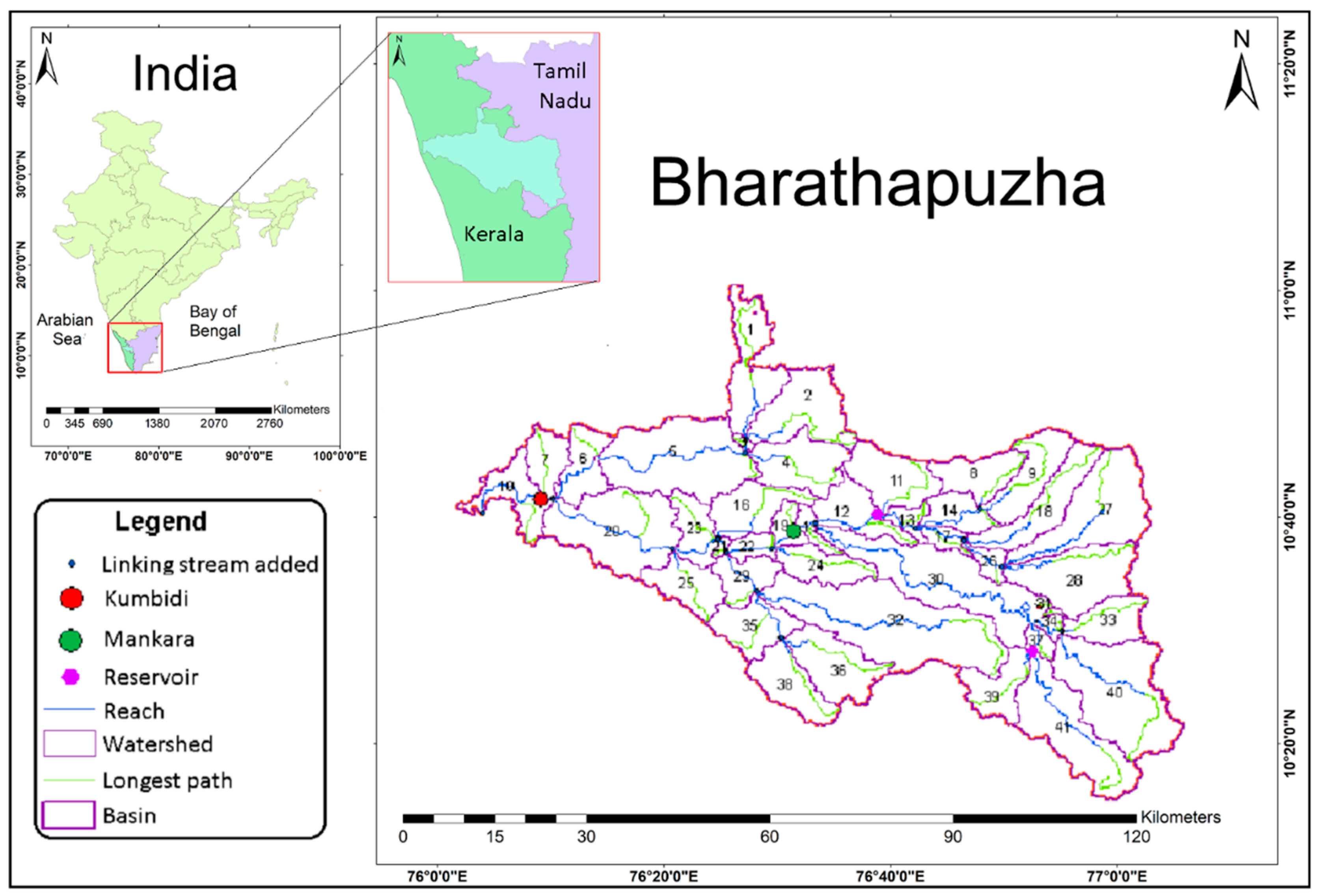
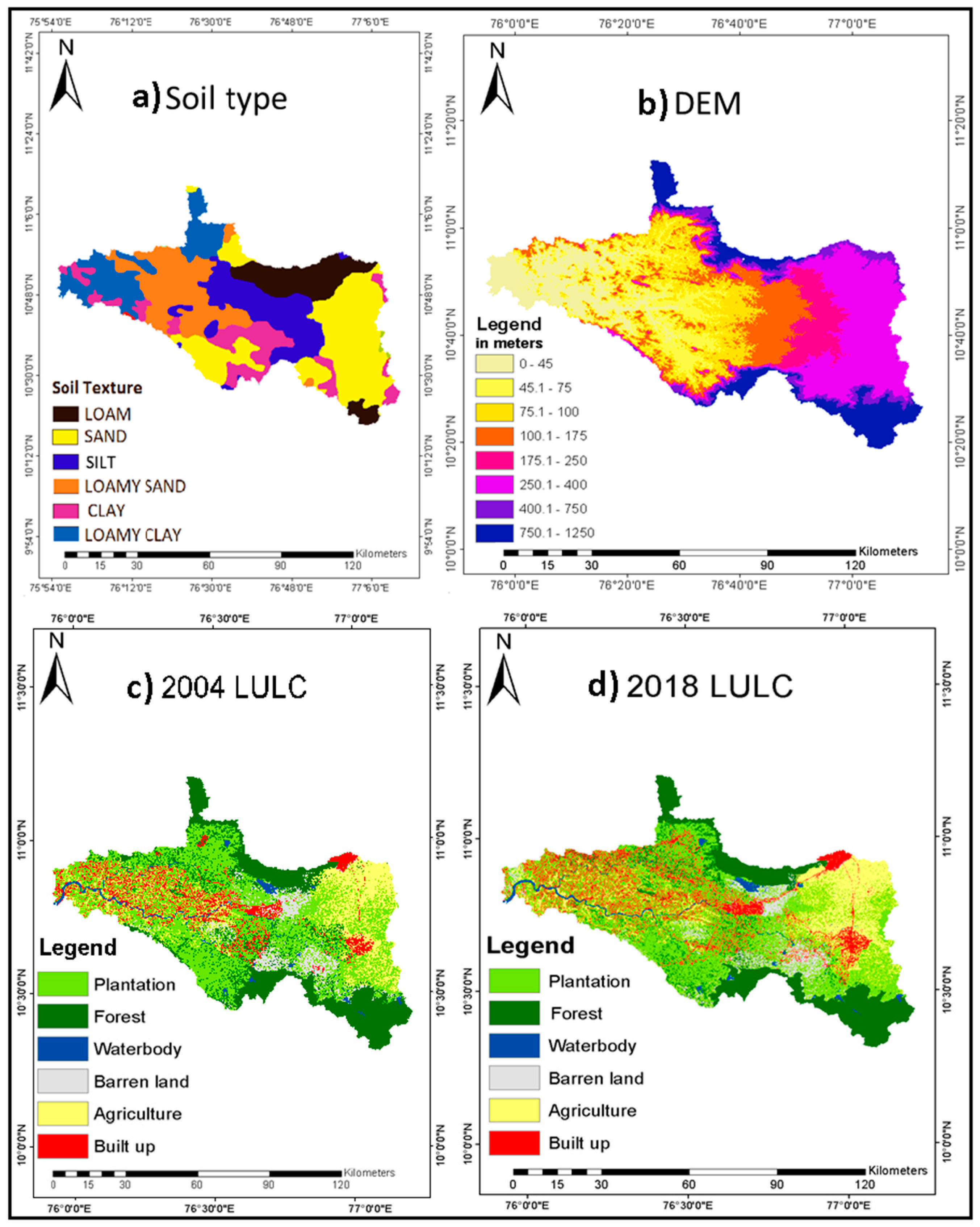
Bharathapuzha River Basin lying in the central part of Western Ghats, India, was chosen as the study area (Figure 1). It has an elevation range between 0 and 1123 m (Figure 2b). It has a total river length of 209 km between source and outlet, with a drainage area of 6186 km2 fed by its four main tributaries, namely Kalpathypuzha, Gayathripuzha, Thootha, and Chitturpuzha. The main river formed by these tributaries finally discharges to the Arabian Sea at Ponnani on the west coast. As per the 2018 land cover analysis (Figure 2d), the basin was mainly covered by forests (20.27%), plantations (45.22%), agriculture (16.1%), built up (10.41%), barren land (5.8%), and waterbody (2.16%).
Two types of crops (paddy and pulse) are typically grown in the area during the two seasons of Kharif (July–November) and Rabi (December–March), respectively. Additionally, arecanut and rubber plantations are predominantly planted in this basin. There are four streamflow gauging stations in the basin, which include Ambarampalayam in Tamil Nadu state and Mankara, Pulamanthole, and Kumbidi in Kerala state. There are three small dams on the upstream side that are used for irrigation water supply in the upstream river basin. They are Walayar, Mamgalam, and Pothundi. Further, there is a big reservoir, Malampuzha constructed in the northern part of Palakkad city that supplies the whole water needed by the city.
The annual precipitation of the BRB in the Western Ghats has decreased over the last 20 years, from 2420 mm in 1981 to 1980 mm in 2010. The rainfall in the study area is contributed mainly by the southwest monsoon, and the average annual precipitation is 2042.3 mm (based on 1971 to 2015 data). Most of the precipitation (approximately 75%) occurs during June to September monsoon months. Further, the average minimum and maximum temperatures of the basin are 23.5 °C and 32.2 °C, respectively. As per the soil map, which was procured from the National Bureau of Soil Survey (NBSS), sandy clay loam and clay loam are predominant (Figure 2a) in BRB. Here, the river basin was divided into 41 sub-basins for hydrological parameter studies (Figure 1). Further, the salient features of the BRB are given in Table 1.
2.2. Data Used
2.2.1. Historical Input Data
The details of the digital elevation model, soil, land cover, and meteorological data, including rainfall and temperature data that are used as inputs for the simulation of the hydrological model, are shown in Table 2. It should be noted that the Landsat data were collected during February month to minimize the effect of cloud cover during the non-monsoon period. This helped in preparing accurate LULC maps during supervised classification, as shown in Figure 2c,d.
The relative humidity, solar radiation, and wind velocity data collected from Climate Forecast System Reanalysis (CFSR) [44] were interpolated to 0.25° at the same grid points as precipitation data. For calibration and validation purpose, the observed runoff was collected from Central Water Commission of India (CWC) on a daily time scale. In this study, two gauging stations, located at Mankara and Kumbidi, were considered for this purpose. The relevant details of the input data, resolutions, and sources are listed in Table 2.
2.2.2. GCM Climate Data
Statistically downscaled climate variables, including precipitation, minimum and maximum temperature, wind speed, and relative humidity, were procured from five Coupled Model Intercomparison Project 5 (CMIP5) [45] using general circulation model (GCM) simulation at daily time steps. These include Beijing Normal University Earth System Model (BNU-ESM) [46], Canadian Earth System Model 2nd generation (CanESM2) [47], Centre National de Recherches Météorologiques (CNRM-CM5) [48], and Max Planck Institute Earth System Model (MPI-ESM MR, and MPI-ESM-LR) [49]. All the five GCMs outputs that were procured during both historic and future periods for this study were downscaled using a kernel regression-based statistical method [50]. The data was on a daily scale, and further details about the data are explained in [50]. Since the product was prepared for the whole Indian subcontinent, it showed some climatological differences at the basin level, due to local geophysical processes. To account for these systematic biases between model-simulated variables and observed values, a bias correction approach had to be performed before further analysis. In this study, the methodology used by [25], a quantile mapping based bias correction (QMBC), was adopted and performed on each grid separately. QMBC is used because it can easily characterize the probability distribution. Further, it can flexibly adjust the tails (ends) of the cumulative distribution frequency (CDF), which is essential before projection [51]. Further, to understand the nature of the bias-corrected data and its error, the spatial averaged temporal correlation of these variables was plotted against IMD historical data before the actual analysis.
2.3. Methodology
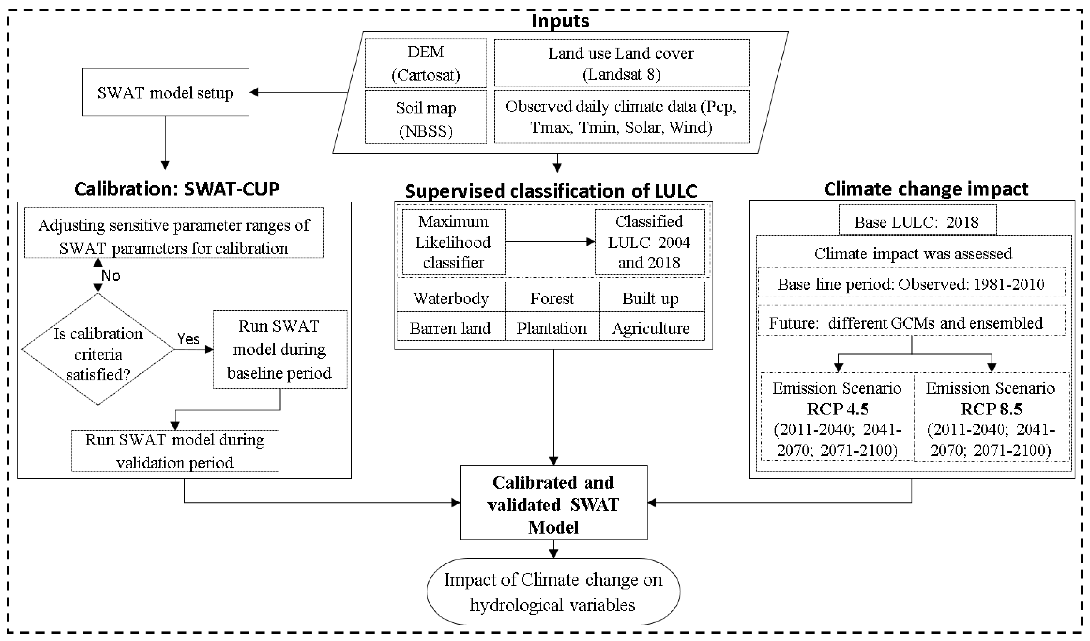
To understand the impact of CC on hydrological variables at the river basin scale in the Western Ghats region, the Bharathapuzha basin located within this region was analyzed using the SWAT model. Before performing the SWAT simulation, all the input data were resampled to the same spatial scale at 0.25°. The details of the hydrological model, LULC preparation, and climate change impact analysis are explained in the subsequent sections. The methodology is shown in Figure 3.
2.3.1. LULC Preparation
Landsat MSS level 2 data was procured from the NASA–USGS database for LULC preparation. Level 2 products were delivered after atmospheric and radiometric correction. Therefore, the data can be used as such, without any preprocessing. For LULC map preparation, a maximum likelihood classifier was used under a supervised classification approach provided within ERDAS Imagine software. Six major classes were identified in the current study area, namely plantation, waterbody, agriculture, barren land, built up, and forest. For calibration of the SWAT model, the 2004 LULC map was prepared (Figure 2c) because it lies within the calibration–validation period to reflect the realistic situation. Further, the 2018 LULC map was prepared and was used as the base map during the base period (1981–2010) for CC impact analyses during the future time period (Figure 2d). The overall accuracy in both the LULC maps was more than 80% during supervised classification.
2.3.2. Climate Change Analysis
Climate change impact assessment for projected future scenarios was analyzed for the entire basin on variables including surface runoff, soil moisture, and evapotranspiration. The projection was performed under two RCP scenarios, namely 4.5 (representing the normal case) and 8.5 (representing severe degradation in atmospheric conditions). Further, the analysis was performed at three levels in the future. (a) Near future (NF) ranging between 2011 and 2040, (b) mid-future (MF) between 2041 and 2070, and (c) far future (FF) between 2071 and 2100. Additionally, the outputs from the five GCMs were analyzed separately to understand the nature of each GCM product on the catchment dynamics. Further, to minimize the effect of epistemic uncertainty, an ensemble averaging technique of all the GCMs was determined for all the variables following [25].
2.3.3. SWAT Model Description
SWAT is a physics-based distributed continuous hydrological model, mainly developed to understand the hydrological physics of a catchment [42]. The model allows the user to perform the model preprocessing by merging with ArcGIS/QGIS platform. Because of this reason, it has been extensively used in various studies related to the different aspects of the hydrological component [52,53]. This includes climate change and LULC change impacts on the hydrological variables [54,55,56,57,58,59]. The success of the proper implementation of the model lies in the identification of the precise value of the model parameters. For this purpose, SWAT provides an algorithm called sequential uncertainty fitness (SUFI-2) to effectively calibrate and validate the model by identifying the sensitive parameters from the available global parameter space. In the current study, 10 parameters were identified as sensitive parameters. Based on the sensitivity results obtained, the SWAT model was calibrated for the two gauging locations from 1993 to 2000, followed by validation for the period from 2001 to 2013. It should be noted that LULC generated for the year 2004 was used as the base map, and other variables, such as DEM and soil, were assumed to be static during the calibration and validation period. Further details about the model can be obtained from Gassman et al. [60]. To evaluate the performance of the model, Nash–Sutcliffe efficiency (NSE) [61], percentage bias (PBIAS) [62], and correlation coefficient (R2) [63] were determined. It should be noted that the SWAT model was run at a monthly time step.
3. Results
3.1. GCM Data Analysis
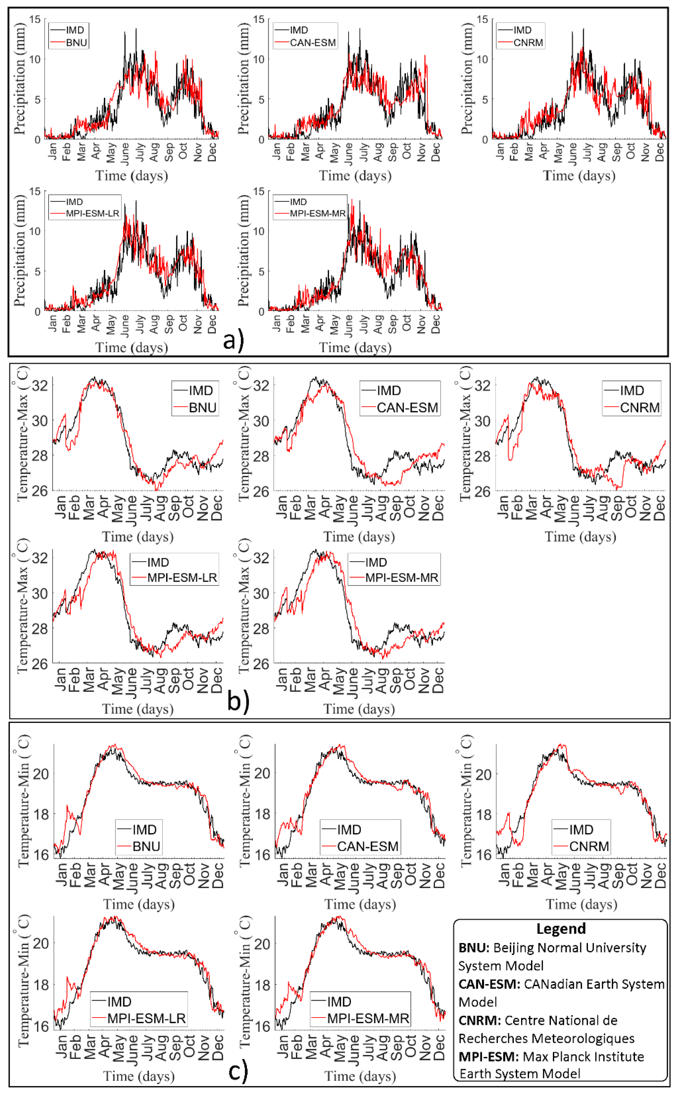
To understand the agreement between the observed and GCM-simulated climate variables at a monthly scale for the BRB, before incorporating it into the SWAT model, a statistical analysis was determined and illustrated in Table 3 below. All the GCM model results, in general, have been clustered together because all the GCM outputs were from the same modeling center. For precipitation data, in particular, the model results were marginally away from the observed point. Still, the NSE and R2 values were around 0.75 to 0.85, which shows that the GCM models can capture the overall trend reasonably well. However, the model-simulated maximum and minimum temperatures had a significant correlation of more than 0.9 value. In addition, the peaks of both variables captured the observation very well, and they were correctly reflected in the NSE values.
In addition, to visually interpret the correlation of GCMs variables with the observations, the long-term monthly averaged observed data were compared with long-term monthly averaged GCM-simulated data from 1981 to 2010. It should be noted that the time series data represented in Figure 4 is an average value of all grids lying within the BRB. From Figure 4, it can be seen that the GCMs could successfully represent the rainfall and temperature climatology after applying the bias correction. Hence, the downscaled variables satisfactorily represent the climatic conditions of the study area and can be further used in the SWAT model, for further simulation.
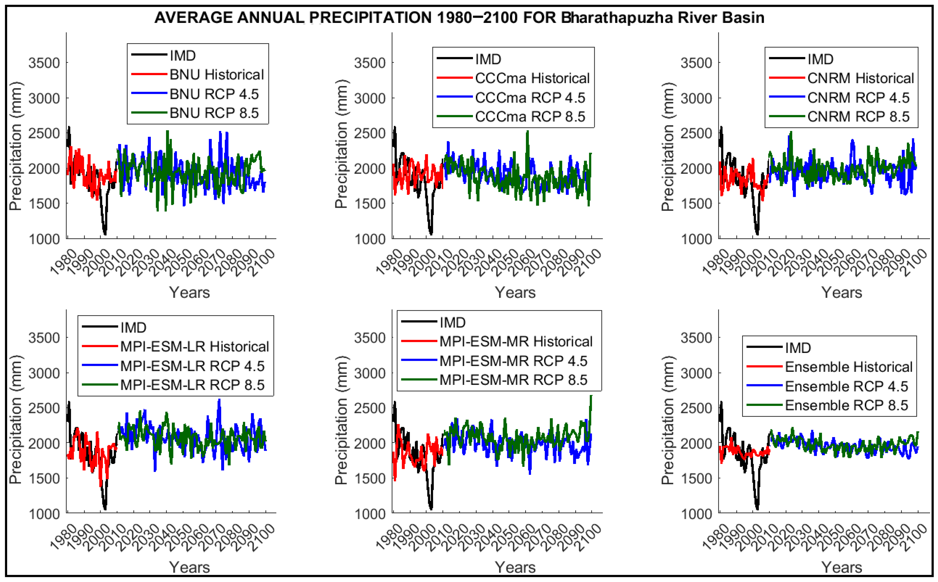
From the historical analyses, it is understood that the bias-corrected data is sufficiently representing the observation trends. Hence, it can be used in the future for further analysis. However, to visually interpret the future trend of these variables during different RCP scenarios, a time series plot was prepared, as shown in Figure 5, Figure 6 and Figure 7. Subsequently, a time series of all the GCMs and an ensemble case from 2011 to 2100 for both the RCP 4.5 and 8.5 scenarios were plotted. Apart from future periods, Figure 5, Figure 6 and Figure 7 also show the time series plots of historical IMD rainfall and maximum and minimum temperature, respectively, with historical GCMs variables from 1981 to 2010. From Figure 5, it can be seen that the rainfall pattern and the magnitude of all GCMs, as well as the ensemble case, are showing a slightly increasing trend for historical and projected future GCMs for both the future RCP 4.5 and 8.5 emission scenarios. It should be noted that, during the historical period (2005), there was a sudden dip in the IMD observed value. Otherwise, the overall trends between both values were consistent with the observed values.
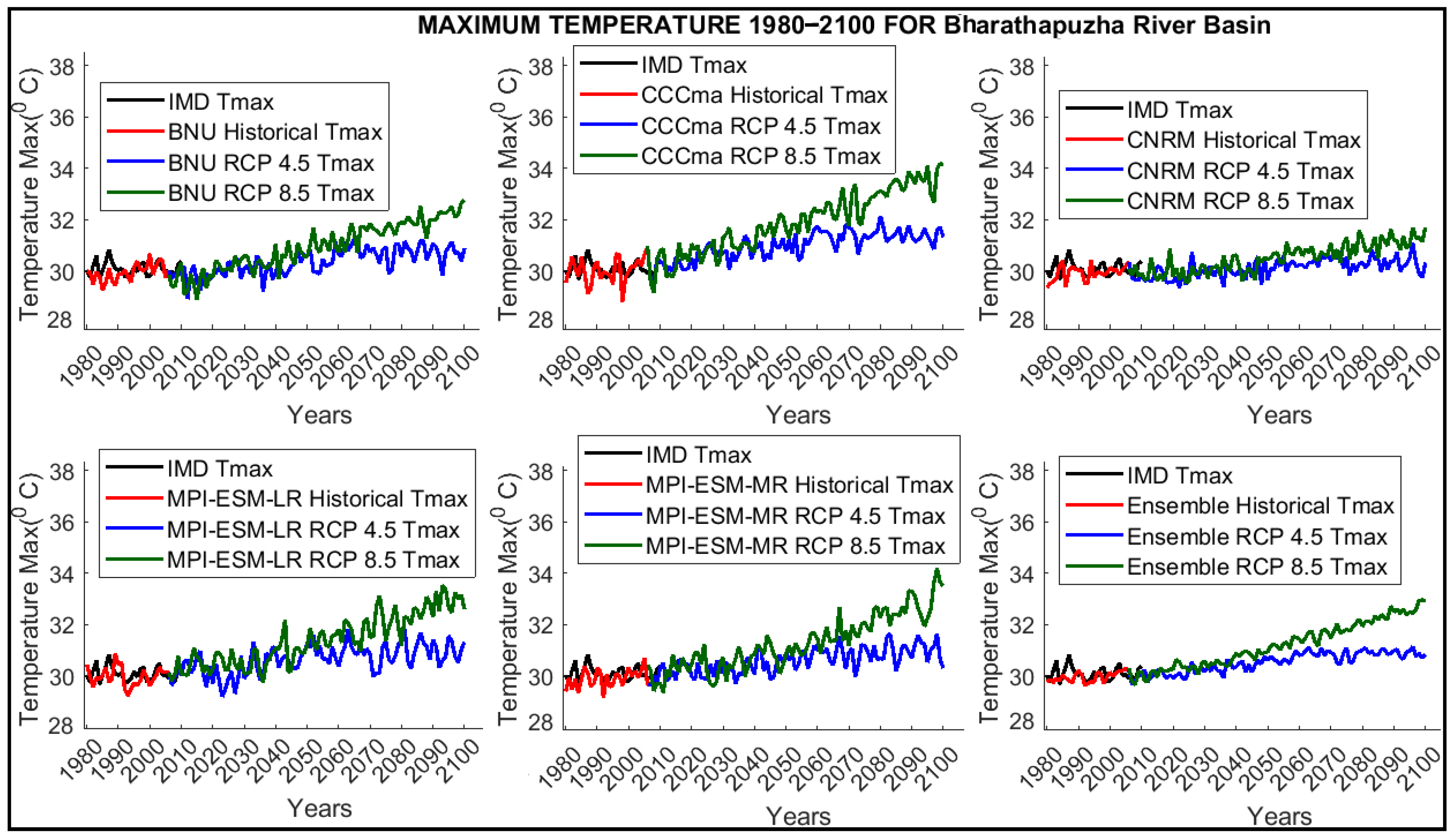
Figure 6 gives a comparison of the maximum temperature (Tmax) from IMD and the maximum temperature of different GCMs, including the ensemble case. All the trends show a very good correlation. The future maximum temperature of RCP 4.5 and 8.5 for all five GCMs, as well as the ensemble case, indicated that the RCP 8.5 scenario will have a maximum temperature of 2 to 4 degrees Celsius more than the RCP 4.5 scenario. The trend for both RCP 4.5 and 8.5 for maximum temperature is acceptable for the future time period.
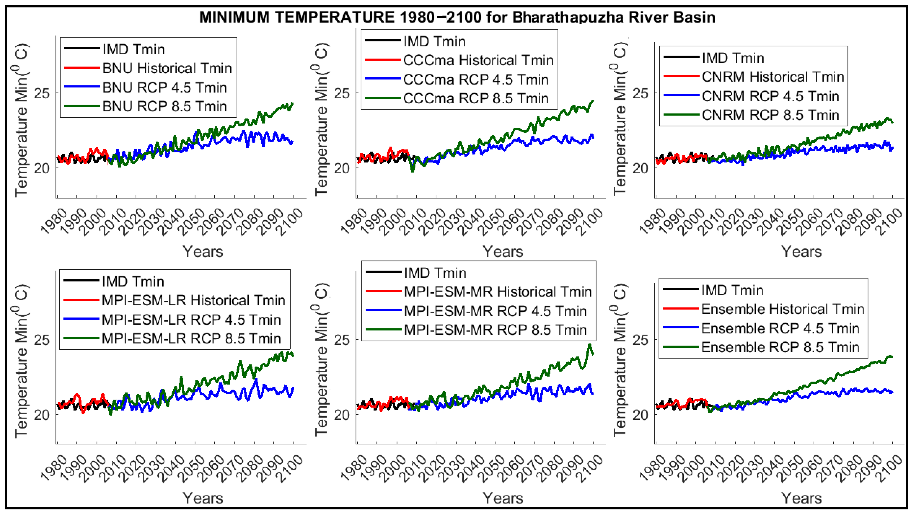
Similarly, the minimum temperature (Tmin) time series plot for the historical and future time periods is plotted in Figure 7. It also shows a good correlation with IMD observed data. Both Figure 6 and Figure 7 show an acceptable range for future maximum and minimum temperatures for BRB after bias correction. Hence, these data can be used for the estimation of hydrological simulations in the basin.
3.2. Calibration and Validation of the SWAT Model
SWAT simulation in the current study was conducted on a monthly scale. The topography (DEM) was used for the delineation of the basin into several sub-basins. The automatic watershed delineation tool of ArcGIS calculates the stream densities and divides the area based on topographical characteristics. The number of sub-basins resulting from the automatic delineation was adjusted by adding/deleting the outlets to adequately delineate the watershed for the hydrologic simulation [64]. The model was first run using a five-year warm-up period, from 1986 to 1990. Table 4 lists the sensitive parameters, with the minimum, maximum, and fitted values used for calibration.
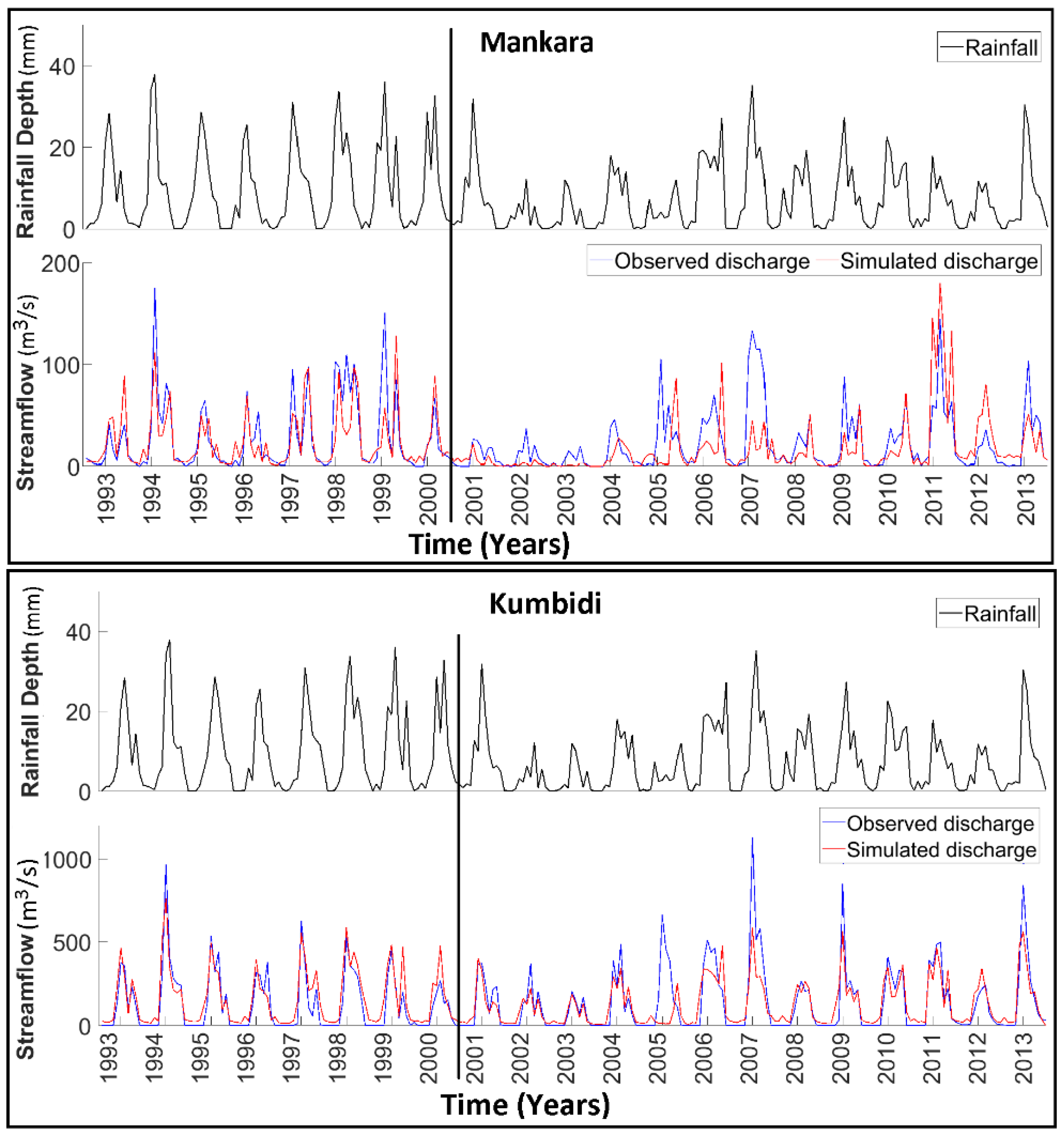
In the BRB, there are four gauging stations, as mentioned in Section 2. However, for the current study, two gauging stations, namely Kumbidi (downstream end) and Mankara (central region), were used during the calibration of the SWAT model. By considering these two gauging stations within the basin, spatial variability can also be accounted for, which is helpful during climate change impact. It is because both the gauging stations represent different climatologies of the basin. The observed and simulated monthly calibration period (1991–2000) and validation period (2001–2013) for streamflow are plotted in Figure 8. From the results, it can be observed that both the R2 and NSE values for streamflow were greater than 0.75 during the calibration and validation periods, which suggests good model performance (Table 5), according to [62].
From Figure 8, it can be observed that the trends between the simulated and observed discharges were well-captured in both gauging locations. This shows that the SWAT model has simulated the spatial variability of the hydrological responses, such as streamflow. Further, from Table 5 it can be seen that model simulation was well-correlated with the observations. The NSE and R2 value were more than 0.7 consistently during both the calibration and validation periods.
3.3. Assessment of Climate Change Impact on Hydrological Variables
3.3.1. Precipitation
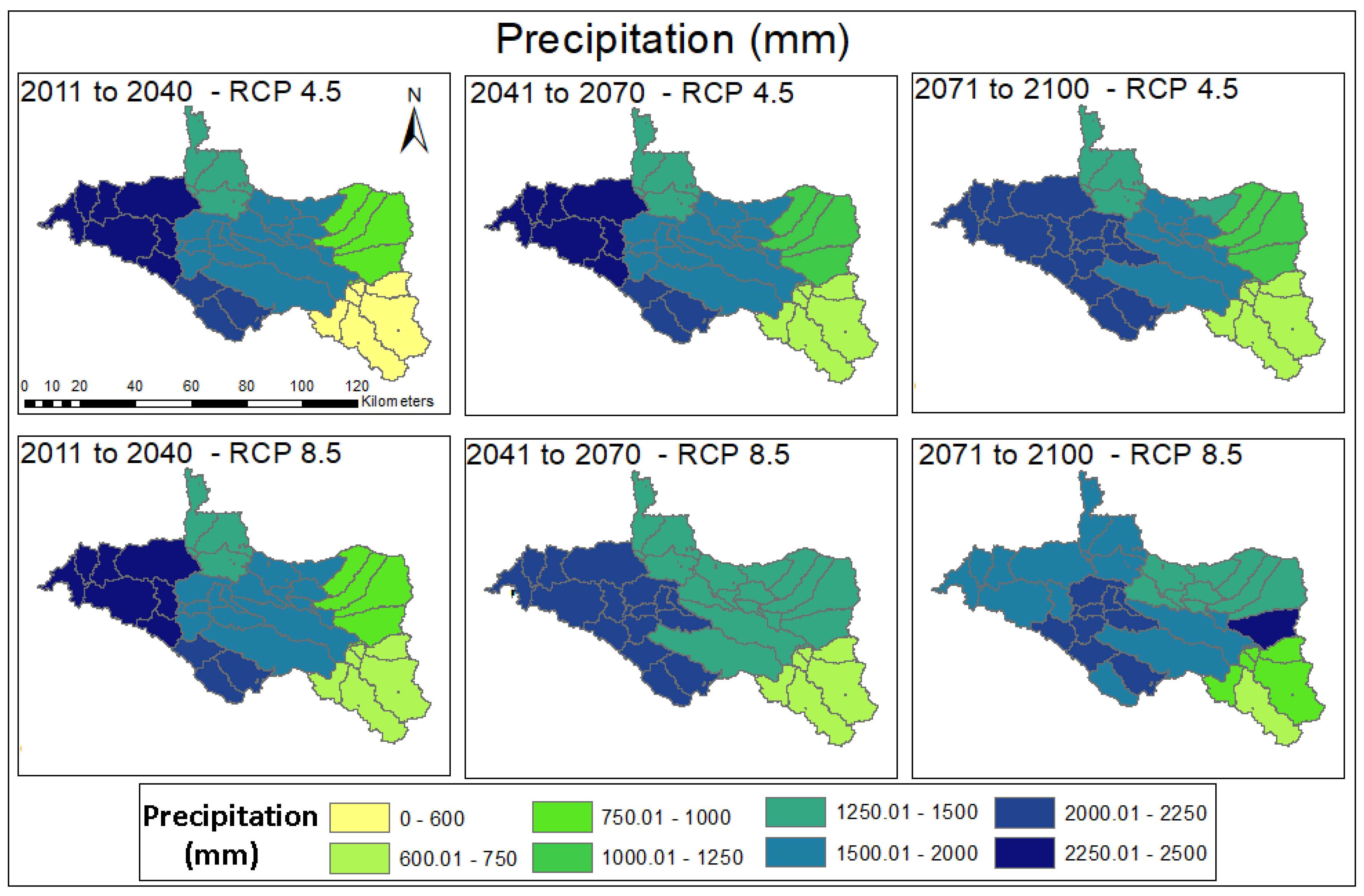
Figure 9 shows the spatial distribution of the precipitation data projected from five GCMs ensembled for the different time slices. From Figure 9, it is understood that, in the future, the rainfall distribution will be more in the downstream areas of the coastal region and less in the upstream areas lying in the Tamil Nadu state. This shows the strong heterogeneous nature of the basin. Rainfall values vary predominantly between 600 and 2500 mm in the BRB, but this trend increases slightly when compared with the historical rainfall trend. When compared between the two scenarios, it is clear that RCP 8.5 showed more increase in the rainfall value than RCP 4.5. Using these rainfall projections and other climatological variables, such as temperature, solar radiation, etc., the SWAT model was run to assess their impacts on the hydrological variables.
3.3.2. Evapotranspiration (ET)
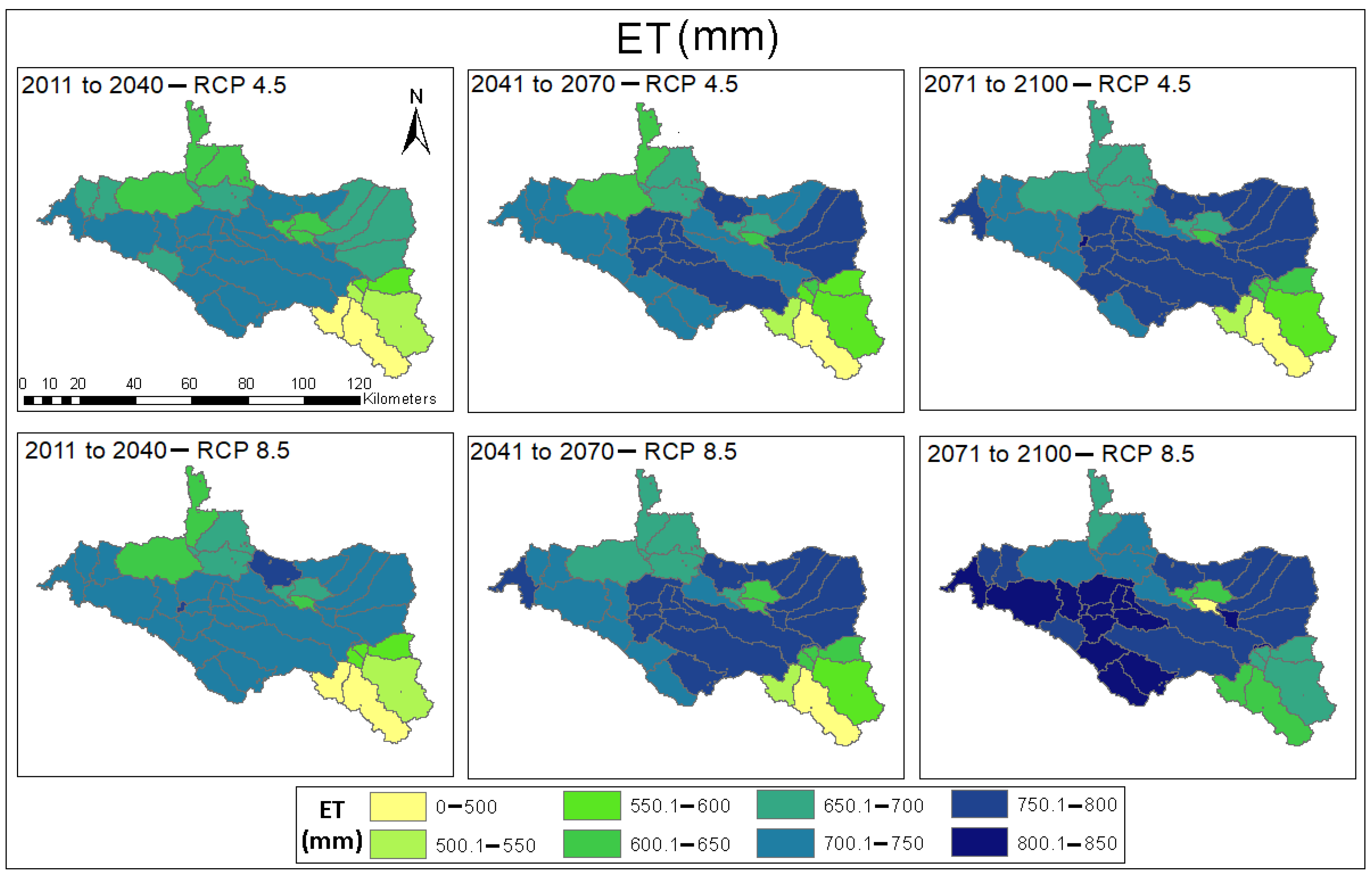
The ET, in general, depends on the rainfall, temperature variation, and land use types of the study area (or given sub-basin). In the Bharathapuzha basin, ET is expected to increase more in the downstream areas and central parts, as compared to the upstream and hilly regions. This is because of the high rainfall pattern and more plantation and agriculture in the respective areas (or sub-basin). In addition, there is deforestation in the hilly region that contributed to less ET value in those sub-basins near the upstream end. Figure 10 also shows a slight increasing trend in ET along different time periods and RCPs scenarios. This may be because of an increase in rainfall and temperature values in the future time period.
3.3.3. Soil Moisture (SM)
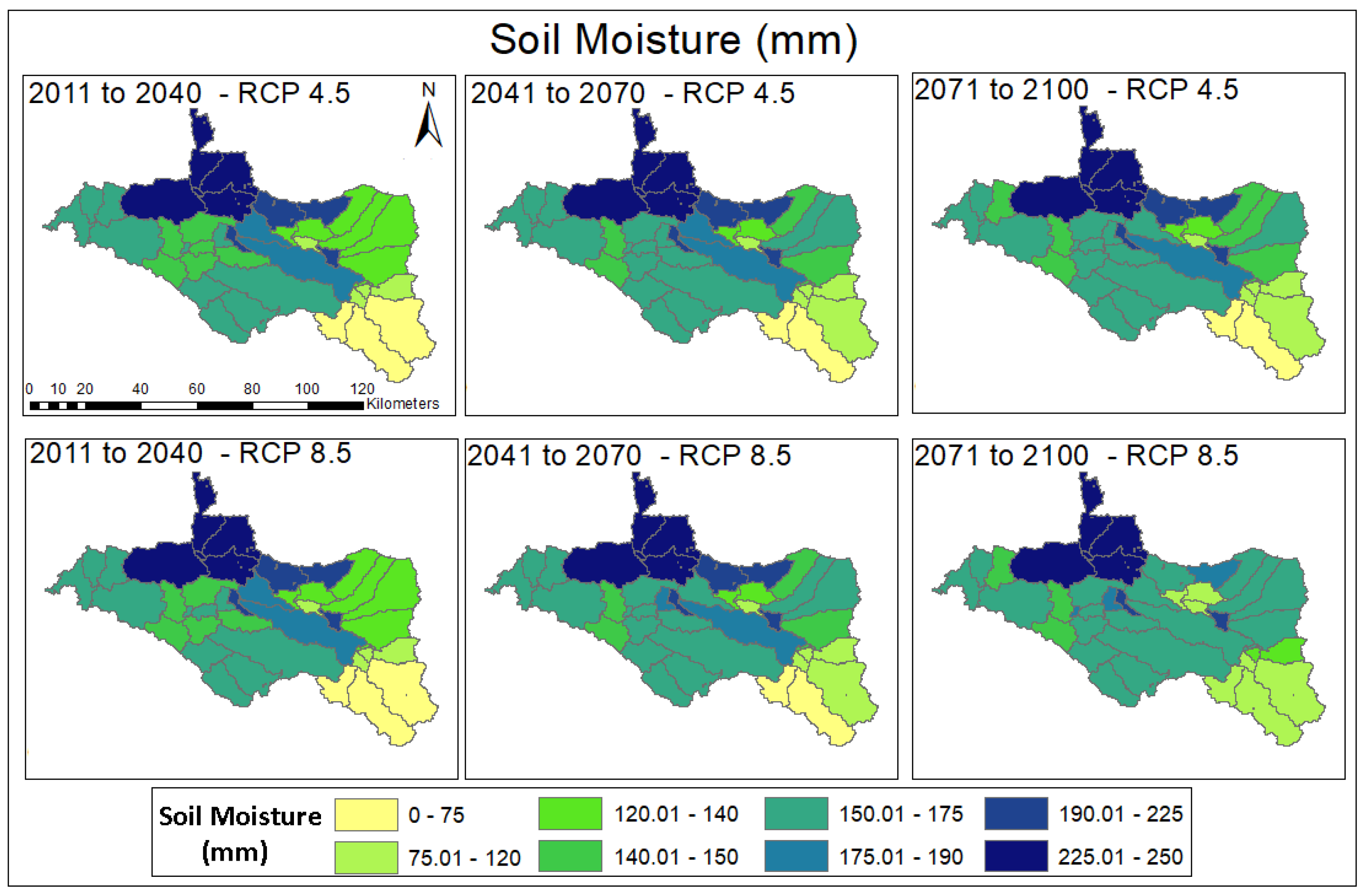
Soil moisture is considered one of the important variables in the hydrometeorological field because it acts as the bridge between the surface and the lower atmosphere [65,66]. Therefore, spatial variations are plotted (Figure 11) for both scenarios. From Figure 11, it is clear that the SM variation between the sub-basin reflects a similar pattern, as shown by the rainfall (Figure 9). Further, it can be noticed that the SM condition is predominantly present in the high terrain in the north, where the vegetation cover is relatively high, and in the coastal region, where precipitation is high. In addition, the changes in the SM conditions from the near and far future are relatively marginal, as compared to the ET variation.
3.3.4. Streamflow (Q)
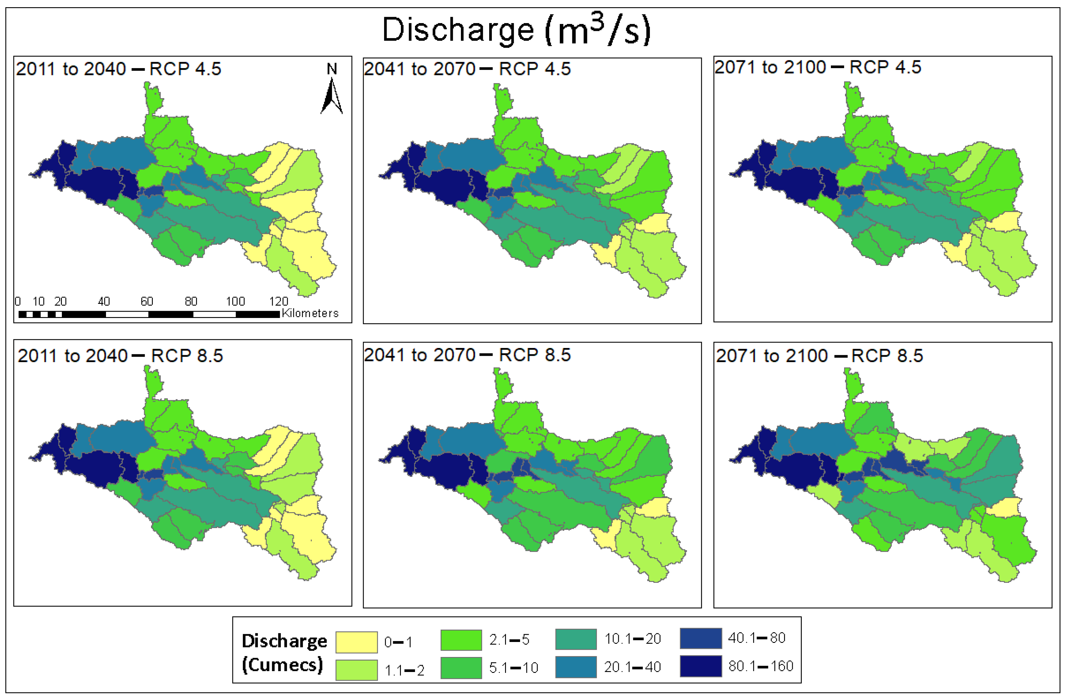
Figure 12 shows the spatial distribution of the discharge during the future period. From Figure 12, it is understood that Q is more dominant in the downstream part of the basin, followed by the central region. However, the upstream end showed a lower streamflow value in the future time periods. In the coastal area, Q reached a value of more than 100 (m3/s), whereas in the upstream region lying on the Tamil Nadu side, Q was less than 10 (m3/s). The major reason behind this is the rainfall and ET pattern over the basin in the future time period (refer to Figure 9 and Figure 10). Another reason for this trend is the accumulation of water over each sub-basin from the upstream side to the downstream end. Further, the spatial plot of the streamflow showed consistency with the rainfall spatial plot, as shown in Figure 9. Past studies also stated that rainfall distribution over a region (sub-basin) heavily influences the streamflow pattern.
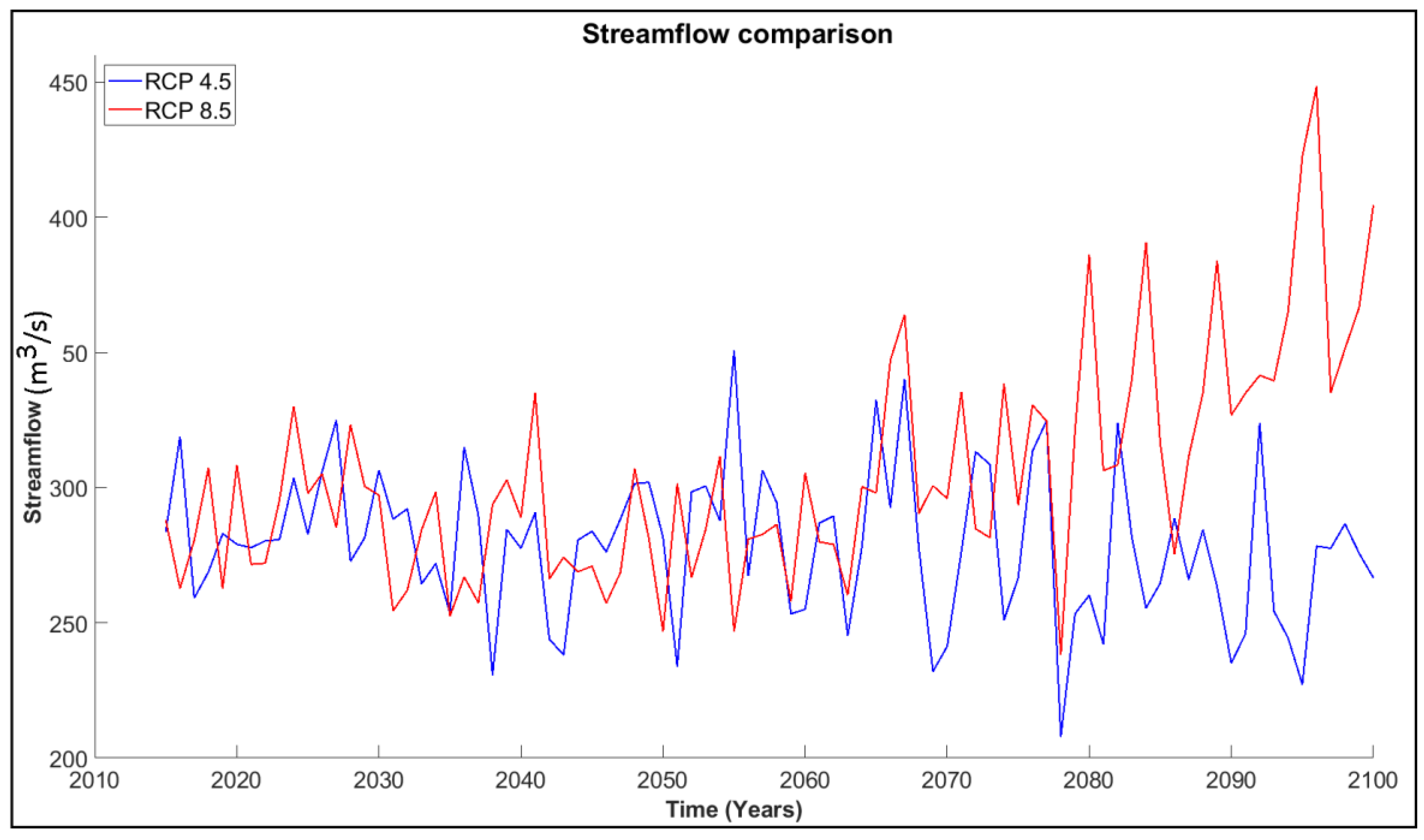
Figure 13 shows an intercomparison of the streamflow time series at the basin outlet for RCP4.5 and 8.5 scenarios for the future time period. From the time series plot, it is clear that there will be a moderate increase in the streamflow trend during future time periods. Further, the average streamflow trend is expected to increase in most of the sub-basins in the future. The magnitude of the increment is significant in the RCP 8.5 scenario. From 285 (m3/s) during base period, it surpassed 400 (m3/s) in the year 2100. In addition, the difference between the RCP 4.5 and 8.5 streamflow is visible during the far future time period. From these two plots, it is expected that the discharge may increase in most of the sub-basins for the Bharathapuzha basin. Especially, the coastal region will experience more impact, due to the changes in the climatic conditions.
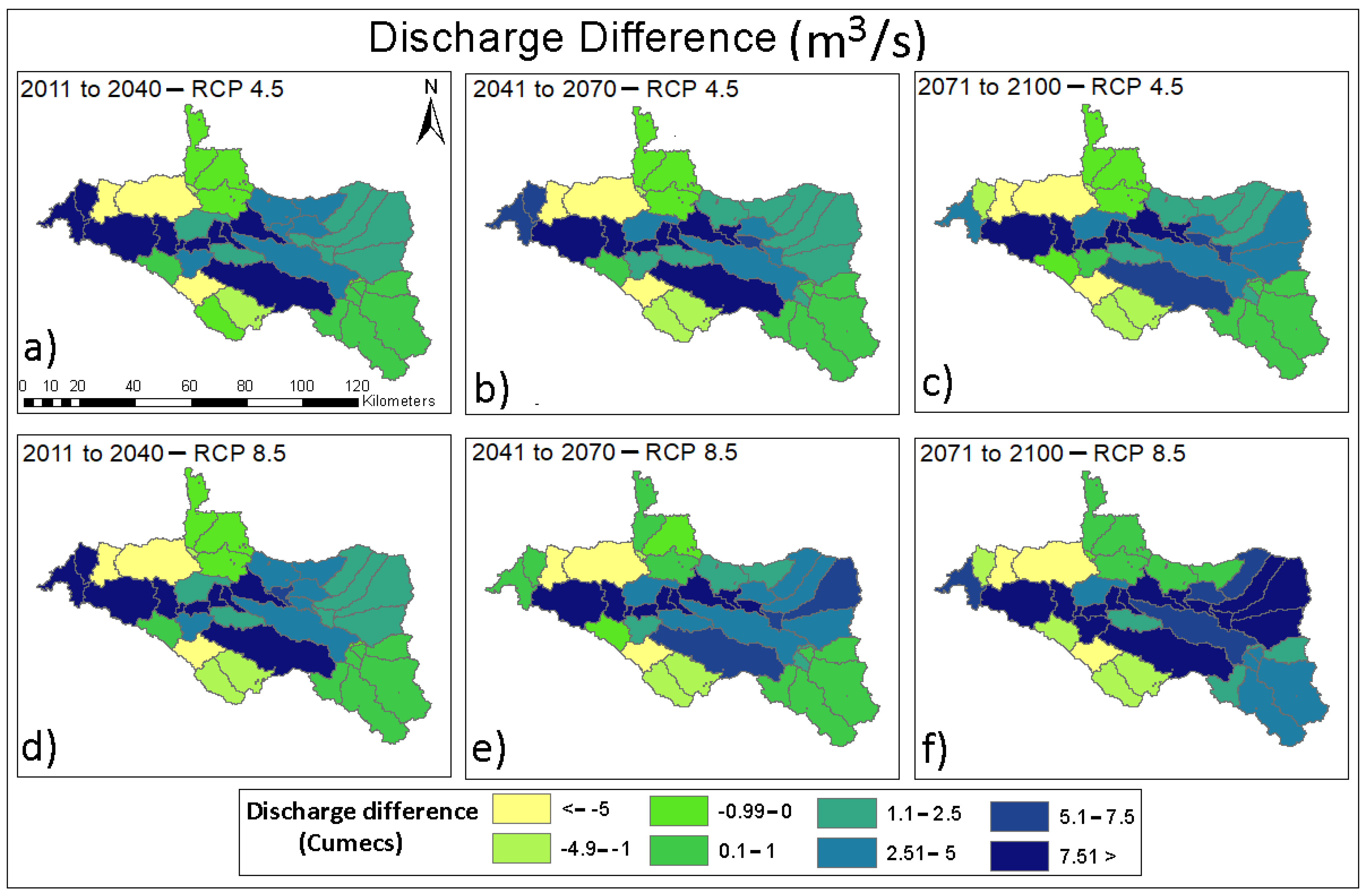
To understand the streamflow variation, with respect to the average value of the baseline period (1981–2010), the spatial distribution of the changes in the future streamflow for different time slices is plotted in Figure 14. The results of the spatial distribution for RCP 4.5 and 8.5 clearly show that only a few sub-basins are indicating a decreasing trend for Q, while most of the other sub-basins are showing a significantly increasing trend, up to 20.22 (m3/s) in the near future, 19.56 (m3/s) in the mid-future, and 17.59 (m3/s) in the far future for RCP 4.5 scenario while similar and more significant results were found in RCP 8.5 scenario. This includes 21.15(m3/s) in near future, 31.93 (m3/s) in the mid-future, and 43.32 (m3/s) in far future time periods. Further, these increases in the streamflow values are predominantly seen in the sub-basins that are near the main river. These results of streamflow’s increasing trend in both the RCPs scenarios and all three future time periods, in comparison to the baseline period (1981–2010), indicate that there is a need for intervention in water resource management in the basin.
To analytically understand the increase in streamflow, with reference to the baseline period (1981–2010), Table 6 is tabulated as shown below. From this table, it is understood that mid-future and far future, under RCP 8.5, experience severe changes, as compared to other scenarios.
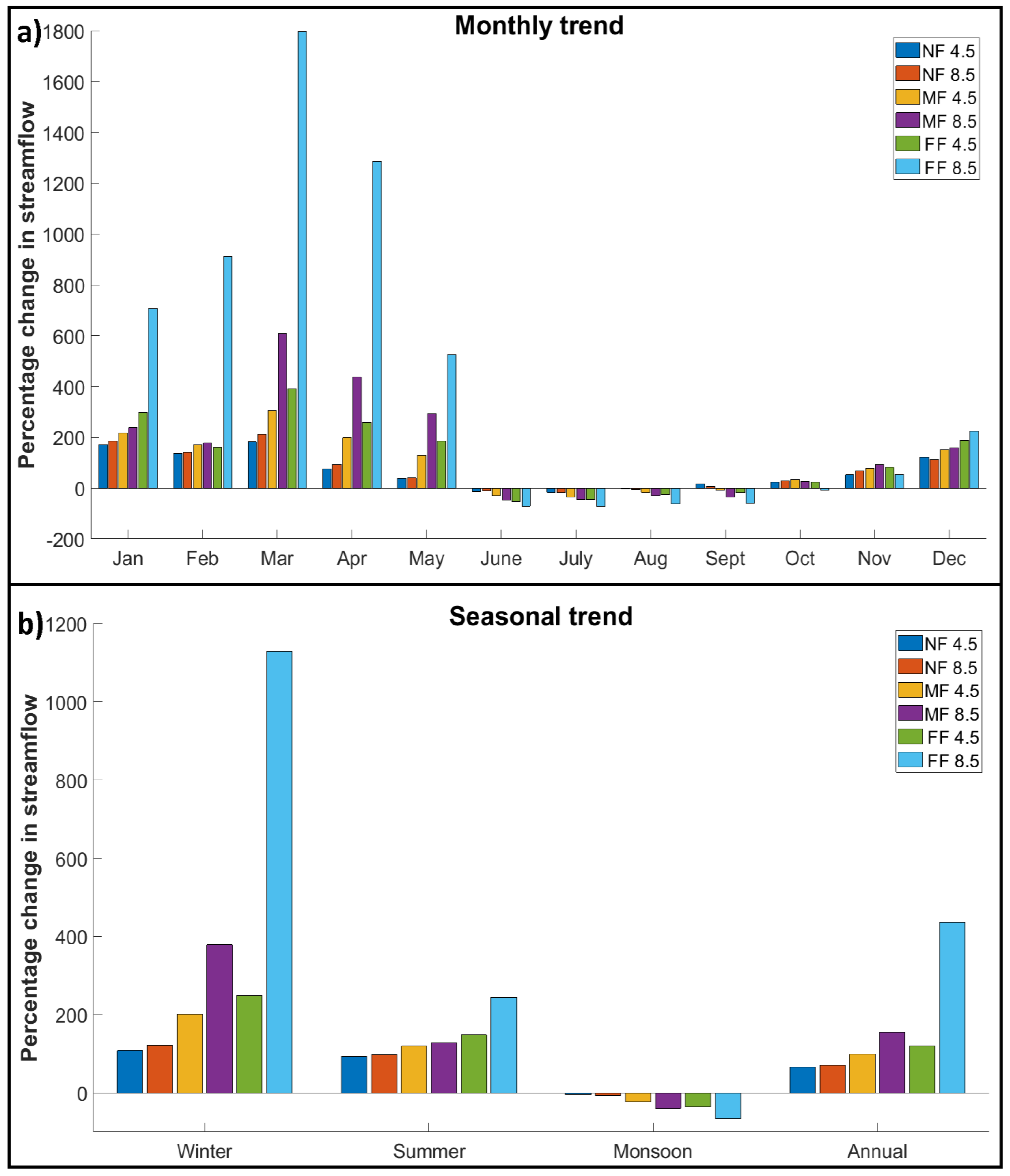
For further analyses, the changes within the monthly, seasonal, and annual streamflow are presented in Figure 15a,b, respectively. From Figure 15a, it can be seen that there was a considerable increase in streamflow from the November to May months and a marginal decrease in the June, July, and August months under both the RCP 4.5 and 8.5 emissions. It was also observed that the increasing trend was more significant, compared to the decreasing trend. For instance, the percentage increase reached values from 120% to 230% during the summer season, whereas the percentage decrease was only marginal and ranged from 15% to 85% during the monsoon season.
Figure 15b represents seasonal change and confirms more clearly the change in the streamflow due to climate change in the future. It clearly shows an increasing trend in the winter and summer seasons and a decreasing trend in the monsoon season. This shows that the streamflow is generally more sensitive towards precipitation change and temperature change. As stated, the increasing annual Q could be due to the increased precipitation trend in the Bharathapuzha basin (refer to Figure 10). Due to extreme climate conditions prevailing in the future, the wetter season (monsoon) is becoming less wet, while the summer and winter seasons, which usually receive less rainfall, become significantly wetter in the future period. This contrary behavior of the climate, as compared to the current situation, is a serious phenomenon that needs to be dealt with in BRB. Further, Q in this region is closely related to ecosystem health, as well. Hence, a new paradigm of water resource management that considers future climate change and the potential increasing streamflow is required.
4. Discussion
Based on the observations, findings, and impacts of climate change on hydrological variables, an assessment of spatiotemporal variability on BRB has been performed. The prediction of these variables gives an idea of the water component within the catchment, which, in turn, will be influential during the sustainable water resources planning and adaptation measures. The changes in the water budget lead to an increase or decrease in the water level. In this study, based on the result, it can be seen that there is a significant increase in the water resource at both the surface level, in terms of streamflow, and at the subsurface level in the form of soil moisture. The sub-basin level spatial analysis also reveals that the downstream end may face an increasing surface runoff and soil moisture level. This correlation was anticipated, given that there would be a substantial increase in the rainfall at the respective sub-basins. On the other hand, the upstream end with relatively flat terrain and the densely populated area are seen to witness a reduction in the water storage levels at both the surface and subsurface levels. This may lead to a shortage of water availability, leading to water stress for domestic, industrial, and agricultural purposes. In addition, the results obtained in this study broadly agree with the past studies [67,68], which primarily emphasized the Indian monsoon in the future. These studies also have highlighted that, at the country scale, the rainfall pattern is expected to shift, due to ongoing global warming. Additionally, the rainfall showed a strong relationship with the increasing temperature around the Indian subcontinent. All these factors also greatly alter the available water resources, as shown in this current study. So, the implementation of proper adaptation measures is warranted, to combat the upcoming drastic changes in Indian water resources.
Sharannya et al. and Sinha et al. [24,25] also performed LULC and climate change impact studies on the adjacent basins of the Western Ghats region and concluded that changes in the local climatic conditions influence the water balance components directly. In this regard, in the Bharathapuzha river basin, rainfall, and temperature are increasing in the future in all-time slices (near, mid, and far). The ET, water yield, and surface runoff trends in all three slices in the future were nearly similar. A similar finding was also reported by Chandu et al. [32], who ran the model at a regional scale using the VIC model. Based on these findings, the ET, water yield, and surface runoff were predicted and can be used for developing decentralized policy at the sub-basin scale. This will simplify land and water management in the river basin and help to improve water availability.
Apart from the impact of climate change on the hydrological variables, LULC changes also play a role in the catchment regime in the future. With the growing population, urban and plantation areas are expected to increase at the cost of forest area, and this will have some impact on the water retention capacity in those areas, leading to changes in soil moisture and runoff components. However, it should be noted that the previous studies conducted in the Western Ghats region [25,35] showed that the impact of CC was predominant, and the effect of LULC change on hydrological components was not significant. Further, the existing approaches used for LULC projections initiate some uncertainty, and this adds to the existing modeling uncertainty in the future. This study is a first step toward estimating the responses of streamflow in the BRB to projected climate changes. Therefore, a further study needs to be analyzed in detail, as well as incorporate these factors prior to the adaptation measures.
5. Summary and Conclusions
In this study, the impacts of climate change on the streamflow, SM, and ET of the Bharathapuzha river basin have been investigated. Data obtained from five downscaled GCM climate models (BNU-ESM, Can-ESM, CNRM, MPI-ESM MR, and MPI-ESM LR) were used during the historic and future time periods (1981–2100). For future projections, different scenarios of RCP 4.5 and RCP 8.5 were considered to analyze the dynamics of climate change. A SWAT hydrological model was used to simulate the hydrological variables, when forced with the aforementioned GCM data. From the SWAT modeling results, it is understood that, compared to the present condition, the average ET is expected to increase in the future. The increase will be predominantly seen in the downstream and hilly terrain, as compared to the upstream end. Further, spatial analysis was performed at the sub-basin scale to understand the catchment dynamics from the upstream and downstream ends. From the obtained results, it was concluded that the downstream coastal region and central region (Kerala state) are more vulnerable to climate change, in comparison to the upstream region (Tamil Nadu state). Further, the downstream end may witness severe flood situations, due to increased streamflow value. Specifically, it was found that those sub-basins in the downstream end that are especially near to the higher-order streams will be more prone to flood situations in the future. On the other hand, the upstream side may face an acute shortage of water, considering the high percentage of urban population and drier climatic conditions. These conclusions will help government agencies and researchers to identify vulnerable sites easily.
Apart from spatial analyses, basin averaged temporally bisected analyses were also conducted at monthly and seasonal scales. The results indicated an increase in streamflow for the winter and summer seasons and a decreasing trend during the monsoon period for all the future periods under both RCP 4.5 and 8.5 emission scenarios. These results will be critical, and they can be used as input data for various climate change-related management and adaptation measures in the future. The methodology used in the present study can be adopted to other heterogeneous complex basins for future water resource management and adaptations. Yet, the combined impact of LULC and climate change together represent a realistic impression of the catchment response in the future. Therefore, a further study has to be analyzed and incorporate the impact of both future LULC and climate projections on the hydrological variables, including streamflow during the future, such that the adaptation measures taken will be more reasonable.
Author Contributions
Conceptualization: T.I.E. and R.R.; methodology: R.V. and T.I.E.; software: R.R.; validation: R.V.; formal analysis: R.V. and T.I.E.; investigation: R.V.; resources: T.I.E. and R.R.; writing—original draft preparation: R.V.; writing—review and editing: T.I.E., R.R. and M.K.J.; supervision: T.I.E. and R.R.; funding acquisition: T.I.E., R.R. and M.K.J. All authors have read and agreed to the published version of the manuscript.
Funding
This research received no external funding.
Institutional Review Board Statement
Not applicable.
Informed Consent Statement
Not applicable.
Data Availability Statement
Streamflow observations were obtained from Central Water Commission (http://www.indiawris.nrsc.gov.in/) from 1 January 1979 to 31 December 2016 for Kumbidi station and 1 January 1986 to 31 December 2015 for Mankara station. Input meteorological datasets from 1980 to 2015 were procured from Climate Forecast System Reanalysis (CFSR) https://climatedataguide.ucar.edu/climate-data/climate-forecast-system-reanalysis-cfsr, Landsat data was downloaded from (http://earthexplorer.usgs.gov/), and Cartosat data was obtained from National Remote Sensing Centre (http://www.nrsc.gov.in/). All Data accessed on 1 March 2019.
Acknowledgments
The authors would like to express their sincere gratitude to the India Metrological Department and the Central Water Commission for sharing the observed data that helped in the successful running of the hydrological model. Authors extend their thanks to the erstwhile Ministry of Water Resources (MoWR), presently the Ministry of Jal Shakthi, Government of India for the project titled “Impact of Climate Change on water resources in river basins from Tadri to Kanyakumari (INCCC)”. Authors are thankful to Editors, Reviewers and Editorial Board for their constructive comments, which improved the manuscript significantly.
Conflicts of Interest
The authors declare no conflict of interest.
References
- Zhang, Y.; Li, H.; Reggiani, P. Climate variability and climate change impacts on land surface, hydrological processes and water management. Water 2019, 11, 1492. [Google Scholar] [CrossRef] [Green Version]
- Seguis, L.; Cappelaere, B.; Milesi, G.; Peugeot, C.; Massuel, S.; Favreau, G. Simulated impacts of climate change and land-clearing on runoff from a small Sahelian catchment. Hydrol. Process. 2004, 18, 3401–3413. [Google Scholar] [CrossRef] [Green Version]
- Goderniaux, P.; Brouyère, S.; Fowler, H.J.; Blenkinsop, S.; Therrien, R.; Orban, P.; Dassargues, A. Large scale surface–subsurface hydrological model to assess climate change impacts on groundwater reserves. J. Hydrol. 2009, 373, 122–138. [Google Scholar] [CrossRef]
- Kalugin, A.S. The impact of climate change on surface, subsurface, and groundwater flow: A case study of the Oka River (European Russia). Water Resour. 2019, 46, S31–S39. [Google Scholar] [CrossRef]
- Rahmat, A.; Zaki, M.K.; Effendi, I.; Mutolib, A.; Yanfika, H.; Listiana, I. Effect of global climate change on air temperature and precipitation in six cities in Gifu Prefecture, Japan. J. Phys. Conf. Ser. 2019, 1155, 012070. [Google Scholar] [CrossRef]
- Hansen, J.; Ruedy, R.; Sato, M.; Lo, K. Global surface temperature change. Rev. Geophys. 2010, 48, 4. [Google Scholar] [CrossRef] [Green Version]
- Lant, C.; Stoebner, T.J.; Schoof, J.T.; Crabb, B. The effect of climate change on rural land cover patterns in the Central United States. Clim. Change 2016, 138, 585–602. [Google Scholar] [CrossRef]
- Liu, H.L.; Willems, P.; Bao, A.M.; Wang, L.; Chen, X. Effect of climate change on the vulnerability of a socio-ecological system in an arid area. Glob. Planet. Change 2016, 137, 1–9. [Google Scholar] [CrossRef]
- Holman, I.P.; Rounsevell MD, A.; Shackley, S.; Harrison, P.A.; Nicholls, R.J.; Berry, P.M.; Audsley, E. A regional, multi-sectoral and integrated assessment of the impacts of climate and socio-economic change in the UK. Clim. Change 2005, 71, 9–41. [Google Scholar] [CrossRef]
- Ministry of Water Resources of India. Integrated Water Resource Development—A Plan for Action. Report of the National Commission for Integrated Water Resources Development; Government of India: New Delhi, India, 1999; Volume I.
- Gosain, A.K.; Sandhya, R.; Debajit, B. Climate change impact assessment on hydrology of Indian river basins. Curr. Sci. 2006, 90, 346–353. [Google Scholar]
- Mancosu, N.; Snyder, R.L.; Kyriakakis, G.; Spano, D. Water scarcity and future challenges for food production. Water 2015, 7, 975–992. [Google Scholar] [CrossRef]
- Mastrandrea, M.D.; Mach, K.J.; Plattner, G.K.; Edenhofer, O.; Stocker, T.F.; Field, C.B.; Ebi, K.L.; Matschoss, P.R. The IPCC AR5 guidance note on consistent treatment of uncertainties: A common approach across the working groups. Clim. Change 2011, 108, 675–691. [Google Scholar] [CrossRef] [Green Version]
- Arnell, N.W.; Reynard, N.S. The effects of climate change due to global warming on river flows in Great Britain. J. Hydrol. 1996, 183, 397–424. [Google Scholar] [CrossRef]
- Lal, P.N.; Mitchell, T.; Mechler, R. National systems for managing the risks from climate extremes and disasters; Cambridge University Press: Cambridge, UK, 2012; pp. 339–392. [Google Scholar]
- Tsegaw, A.T.; Pontoppidan, M.; Kristvik, E.; Alfredsen, K.; Muthanna, T.M. Hydrological impacts of climate change on small ungauged catchments–results from a global climate model–regional climate model–hydrologic model chain. Nat. Hazards Earth Syst. Sci. 2020, 20, 2133–2155. [Google Scholar] [CrossRef]
- Dibike, Y.B.; Paulin, C. Hydrologic impact of climate change in the Saguenay watershed: Comparison of downscaling methods and hydrologic models. J. Hydrol. 2005, 307, 145–163. [Google Scholar] [CrossRef]
- Dong, C.; Schoups, G.; van de Giesen, N. Scenario development for water resource planning and management: A review. Technol. Forecast. Soc. Change 2013, 80, 749–761. [Google Scholar] [CrossRef]
- Loucks, D.P.; Beek, E.V. Water resources planning and management: An overview. In Water Resource Systems Planning and Management; Springer: Cham, Switzerland, 2017; pp. 1–49. [Google Scholar]
- Ranasinghe, R. On the need for a new generation of coastal change models for the 21st century. Sci. Rep. 2020, 10, 1–6. [Google Scholar] [CrossRef] [Green Version]
- Bamunawala, J.; Maskey, S.; Duong, T.M.; Van der Spek, A. Significance of fluvial sediment supply in coastline modelling at tidal inlets. J. Mar. Sci. Eng. 2018, 6, 79. [Google Scholar] [CrossRef] [Green Version]
- Steele-Dunne, S.; Lynch, P.; McGrath, R.; Semmler, T.; Wang, S.; Hanafin, J.; Nolan, P. The impacts of climate change on hydrology in Ireland. J. Hydrol. 2008, 356, 28–45. [Google Scholar] [CrossRef]
- Sharannya, T.M.; Venkatesh, K.; Mudbhatkal, A.; Dineshkumar, M.; Mahesha, A. Effects of land use and climate change on water scarcity in rivers of the Western Ghats of India. Environ. Monit. Assess. 2021, 193, 1–17. [Google Scholar] [CrossRef] [PubMed]
- Sharannya, T.M.; Mudbhatkal, A.; Mahesha, A. Assessing climate change impacts on river hydrology–A case study in the Western Ghats of India. J. Earth Syst. Sci. 2018, 127, 1–11. [Google Scholar] [CrossRef]
- Sinha, R.K.; Eldho, T.I.; Subimal, G. Assessing the impacts of land cover and climate on runoff and sediment yield of a river basin. Hydrol. Sci. J. 2020, 65, 2097–2115. [Google Scholar] [CrossRef]
- Christensen, N.S.; Wood, A.W.; Voisin, N.; Lettenmaier, D.P.; Palmer, R.N. The effects of climate change on the hydrology and water resources of the Colorado River basin. Clim. Change 2004, 62, 337–363. [Google Scholar] [CrossRef]
- Pilling, C.G.; Jones, J.A.A. The impact of future climate change on seasonal discharge, hydrological processes and extreme flows in the Upper Wye experimental catchment, Mid-Wales. Hydrol. Process. 2002, 16, 1201–1213. [Google Scholar] [CrossRef]
- Prowse, T.D.; Beltaos, S.; Gardner, J.T.; Gibson, J.J.; Granger, R.J.; Leconte, R.; Peters, D.L.; Pietroniro, A.; Romolo, L.A.; Toth, B. Climate change, flow regulation and land-use effects on the hydrology of the Peace-Athabasca-Slave system; Findings from the Northern Rivers Ecosystem Initiative. Environ. Monit. Assess. 2006, 113, 167–197. [Google Scholar] [CrossRef] [Green Version]
- Gosain, A.K.; Sandhya, R.; Anamika, A. Climate change impact assessment of water resources of India. Curr. Sci. 2011, 101, 356–371. [Google Scholar]
- Madhusoodhanan, C.G.; Sreeja, K.G.; Eldho, T.I. Climate change impact assessments on the water resources of India under extensive human interventions. Ambio 2016, 45, 725–741. [Google Scholar] [CrossRef] [Green Version]
- Upgupta, S.; Sharma, J.; Jayaraman, M.; Kumar, V.; Ravindranath, N.H. Climate change impact and vulnerability assessment of forests in the Indian Western Himalayan region: A case study of Himachal Pradesh, India. Clim. Risk Manag. 2015, 10, 63–76. [Google Scholar] [CrossRef] [Green Version]
- Chandu, N.; Eldho, T.I.; Mondal, A. Hydrological impacts of climate and land-use change in Western Ghats, India. Reg. Environ. Change 2022, 22, 1–15. [Google Scholar] [CrossRef]
- Mishra, A.; Singh, R.; Raghuwanshi, N.S.; Chatterjee, C.; Froebrich, J. Spatial variability of climate change impacts on yield of rice and wheat in the Indian Ganga Basin. Sci. Total Environ. 2013, 468, S132–S138. [Google Scholar] [CrossRef]
- Dubey, S.K.; Sharma, D. Assessment of climate change impact on yield of major crops in the Banas River Basin, India. Sci. Total Environ. 2018, 635, 10–19. [Google Scholar] [CrossRef]
- Sinha, R.K.; Eldho, T.I.; Subimal, G. Assessing the impacts of historical and future land use and climate change on the streamflow and sediment yield of a tropical mountainous river basin in South India. Environ. Monit. Assess. 2020, 192, 1–21. [Google Scholar] [CrossRef]
- Sinha, R.K.; Eldho, T.I. Assessment of soil erosion susceptibility based on morphometric and landcover analysis: A case study of Netravati River Basin, India. J. Indian Soc. Remote Sens. 2021, 49, 1709–1725. [Google Scholar] [CrossRef]
- Wagner, P.D.; Kumar, S.; Schneider, K. An assessment of land use change impacts on the water resources of the Mula and Mutha Rivers catchment upstream of Pune, India. Hydrol. Earth Syst. Sci. 2013, 17, 2233–2246. [Google Scholar] [CrossRef] [Green Version]
- Garg, V.; Nikam, B.R.; Thakur, P.K.; Aggarwal, S.P.; Gupta, P.K.; Srivastav, S.K. Human-induced land use land cover change and its impact on hydrology. HydroResearch 2019, 1, 48–56. [Google Scholar] [CrossRef]
- CWC (Central Water Commission). Reassessment of Water Availability in India Using Space Inputs. Basin Planning and Management Organisation; Central Water Commission: New Delhi, India, 2017. Available online: http://www.cwc.gov.in/publications (accessed on 1 March 2019).
- Zuo, D.; Xu, Z.; Yao, W.; Jin, S.; Xiao, P.; Ran, D. Assessing the effects of changes in land use and climate on runoff and sediment yields from a watershed in the Loess Plateau of China. Sci. Total Environ. 2016, 544, 238–250. [Google Scholar] [CrossRef]
- Chawla, I.; Mujumdar, P.P. Isolating the impacts of land use and climate change on streamflow. Hydrol. Earth Syst. Sci. 2015, 19, 3633–3651. [Google Scholar] [CrossRef] [Green Version]
- Arnold, J.G.; Srinivasan, R.; Muttiah, R.S.; Williams, J.R. Large area hydrologic modeling and assessment part I: Model development 1. JAWRA J. Am. Water Resour. Assoc. 1998, 34, 73–89. [Google Scholar] [CrossRef]
- Pai, D.S.; Rajeevan, M.; Sreejith, O.P.; Mukhopadhyay, B.; Satbha, N.S. Development of a new high spatial resolution (0.25 × 0.25) long period (1901–2010) daily gridded rainfall data set over India and its comparison with existing data sets over the region. Mausam 2014, 65, 1–18. [Google Scholar] [CrossRef]
- Dile, Y.T.; Srinivasan, R. Evaluation of CFSR climate data for hydrologic prediction in data-scarce watersheds: An application in the Blue Nile River Basin. JAWRA J. Am. Water Resour. Assoc. 2014, 50, 1226–1241. [Google Scholar] [CrossRef]
- Madhusoodhanan, C.G.; Shashikanth, K.; Eldho, T.I.; Ghosh, S. Can statistical downscaling improve consensus among CMIP5 models for Indian summer monsoon rainfall projections? Int. J. Climatol. 2018, 38, 2449–2461. [Google Scholar] [CrossRef]
- Ji, D.; Wang, L.; Feng, J.; Wu, Q.; Cheng, H.; Zhang, Q.; Yang, J.; Dong, W.; Dai, Y.; Gong, D.; et al. Description and basic evaluation of Beijing Normal University Earth system model (BNU-ESM) version 1. Geosci. Model Dev. 2014, 7, 2039–2064. [Google Scholar] [CrossRef]
- Swart, N.C.; Cole, J.N.; Kharin, V.V.; Lazare, M.; Scinocca, J.F.; Gillett, N.P.; Anstey, J.; Arora, V.; Christian, J.R.; Hanna, S.; et al. The Canadian earth system model version 5 (CanESM5. 0.3). Geosci. Model Dev. 2019, 12, 4823–4873. [Google Scholar] [CrossRef] [Green Version]
- Salas-Mélia, D.; Chauvin, F.; Déqué, M.; Douville, H.; Gueremy, J.F.; Marquet, P.; Planton, S.; Royer, J.F.; Tyteca, S. Description and validation of the CNRM-CM3 global coupled model. CNRM Work. Note 2005, 103, 36. [Google Scholar]
- Gutjahr, O.; Putrasahan, D.; Lohmann, K.; Jungclaus, J.H.; von Storch, J.S.; Brüggemann, N.; Haak, H.; Stössel, A. Max planck institute earth system model (MPI-ESM1. 2) for the high-resolution model intercomparison project (HighResMIP). Geosci. Model Dev. 2019, 12, 3241–3281. [Google Scholar] [CrossRef] [Green Version]
- Kannan, S.; Subimal, G. A nonparametric kernel regression model for downscaling multisite daily precipitation in the Mahanadi basin. Water Resour. Res. 2013, 49, 1360–1385. [Google Scholar] [CrossRef]
- Li, H.; Sheffield, J.; Wood, E.F. Bias correction of monthly precipitation and temperature fields from Intergovernmental panel on climate change AR4 models using equidistant quantile matching. J. Geophys. Res. Atmos. 2010, 115, D10. [Google Scholar] [CrossRef]
- Dechmi, F.; Burguete, J.; Skhiri, A. SWAT application in intensive irrigation systems: Model modification, calibration and validation. J. Hydrol. 2012, 470, 227–238. [Google Scholar] [CrossRef] [Green Version]
- Ndomba, P.M.; Mtalo, F.W.; Killingtveit, Å. A guided SWAT model application on sediment yield modeling in Pangani river basin: Lessons learnt. J. Urban Environ. Eng. 2008, 2, 53–62. [Google Scholar] [CrossRef]
- Bhatta, B.; Shrestha, S.; Shrestha, P.K.; Talchabhadel, R. Evaluation and application of a SWAT model to assess the climate change impact on the hydrology of the Himalayan River Basin. Catena 2019, 181, 104082. [Google Scholar] [CrossRef]
- dos Santos, J.Y.G.; Montenegro, S.M.G.L.; da Silva, R.M.; Santos, C.A.G.; Quinn, N.W.; Dantas, A.P.X.; Neto, A.R. Modeling the impacts of future LULC and climate change on runoff and sediment yield in a strategic basin in the Caatinga/Atlantic forest ecotone of Brazil. Catena 2021, 203, 105308. [Google Scholar] [CrossRef]
- Lu, E.; Takle, E.S.; Manoj, J. The relationships between climatic and hydrological changes in the upper Mississippi River basin: A SWAT and multi-GCM study. J. Hydrometeorol. 2010, 11, 437–451. [Google Scholar] [CrossRef] [Green Version]
- Jha, M.K.; Gassman, P.W.; Panagopoulos, Y. Regional changes in nitrate loadings in the Upper Mississippi River Basin under predicted mid-century climate. Reg. Environ. Change 2015, 15, 449–460. [Google Scholar] [CrossRef]
- Jha, M.K.; Gassman, P.W. Changes in hydrology and streamflow as predicted by a modelling experiment forced with climate models. Hydrol. Process. 2014, 28, 2772–2781. [Google Scholar] [CrossRef]
- Chattopadhyay, S.; Jha, M.K. Hydrological response due to projected climate variability in Haw River watershed, North Carolina, USA. Hydrol. Sci. J. 2016, 61, 495–506. [Google Scholar] [CrossRef]
- Gassman, P.W.; Sadeghi, A.M.; Srinivasan, R. Applications of the SWAT model special section: Overview and insights. J. Environ. Qual. 2014, 43, 1–8. [Google Scholar] [CrossRef]
- Gassman, P.W.; Sadeghi, A.M.; Srinivasan, R. River flow forecasting through conceptual models part I—A discussion of principles. J. Hydrol. 1970, 10, 282–290. [Google Scholar]
- Moriasi, D.N.; Arnold, J.G.; Van Liew, M.W.; Bingner, R.L.; Harmel, R.D.; Veith, T.L. Model evaluation guidelines for systematic quantification of accuracy in watershed simulations. Trans. ASABE 2007, 50, 885–900. [Google Scholar] [CrossRef]
- Legates, D.R.; McCabe, G.J., Jr. Evaluating the use of “goodness-of-fit” measures in hydrologic and hydroclimatic model validation. Water Resour. Res. 1999, 35, 233–241. [Google Scholar] [CrossRef]
- Jha, M.; Gassman, P.W.; Secchi, S.; Gu, R.; Arnold, J. Effect Of Watershed Subdivision On Swat Flow, Sediment, And Nutrient Predictions 1. JAWRA J. Am. Water Resour. Assoc. 2004, 40, 811–825. [Google Scholar] [CrossRef] [Green Version]
- Visweshwaran, R.; Ramsankaran, R.; Eldho, T.I.; Lakshmivarahan, S. Sensitivity-Based Soil Moisture Assimilation for Improved Streamflow Forecast Using a Novel Forward Sensitivity Method (FSM) Approach. Water Resour. Res. 2022, 58, e2021WR031092. [Google Scholar] [CrossRef]
- Huggannavar, V.; Indu, J. Seasonal variability of soil moisture-precipitation feedbacks over India. J. Hydrol. 2020, 589, 125181. [Google Scholar] [CrossRef]
- Menon, A.; Levermann, A.; Schewe, J.; Lehmann, J.; Frieler, K. Consistent increase in Indian monsoon rainfall and its variability across CMIP-5 models. Earth Syst. Dyn. 2013, 4, 287–300. [Google Scholar] [CrossRef] [Green Version]
- Katzenberger, A.; Schewe, J.; Pongratz, J.; Levermann, A. Robust increase of Indian monsoon rainfall and its variability under future warming in CMIP6 models. Earth Syst. Dyn. 2021, 12, 367–386. [Google Scholar] [CrossRef]
Figure 1.
Study area map showing the location of the Bharathapuzha basin, sub-basins, stream networks, and gauging stations (Mankara and Kumbidi).
Figure 1.
Study area map showing the location of the Bharathapuzha basin, sub-basins, stream networks, and gauging stations (Mankara and Kumbidi).

Figure 2.
Map showing the geophysical details of the BRB (a) soil map, (b) digital elevation model (DEM), and (c,d) 2004 and 2018 LULC classified maps.
Figure 2.
Map showing the geophysical details of the BRB (a) soil map, (b) digital elevation model (DEM), and (c,d) 2004 and 2018 LULC classified maps.

Figure 3.
Schematic diagram of the research methodology.

Figure 4.
GCMs climatology (red), compared with observed climatology (black) for monthly: (a) rainfall (top); (b) maximum temperature, (middle), and (c) minimum temperature (bottom) from 1981 to 2010.
Figure 4.
GCMs climatology (red), compared with observed climatology (black) for monthly: (a) rainfall (top); (b) maximum temperature, (middle), and (c) minimum temperature (bottom) from 1981 to 2010.

Figure 5.
Comparison of observed and GCMs simulated rainfall during historical (1981 to 2010) and future periods (2011 to 2100).
Figure 5.
Comparison of observed and GCMs simulated rainfall during historical (1981 to 2010) and future periods (2011 to 2100).

Figure 6.
Comparison of observed and GCMs simulated maximum temperature during historical (1981 to 2010) and future periods (2011 to 2100).
Figure 6.
Comparison of observed and GCMs simulated maximum temperature during historical (1981 to 2010) and future periods (2011 to 2100).

Figure 7.
Comparison of observed and GCMs simulated minimum temperature during historical (1981 to 2010) and future periods (2011 to 2100).
Figure 7.
Comparison of observed and GCMs simulated minimum temperature during historical (1981 to 2010) and future periods (2011 to 2100).

Figure 8.
Comparison between the observed and simulated streamflow value during the calibration (1993–2000) and Validation (2001–2013) period for Mankara (Top) and Kumbidi (Bottom) gauging stations.
Figure 8.
Comparison between the observed and simulated streamflow value during the calibration (1993–2000) and Validation (2001–2013) period for Mankara (Top) and Kumbidi (Bottom) gauging stations.

Figure 9.
Spatial distribution of rainfall for near, mid-, and far future of RCP 4.5 and 8.5 emission scenarios.
Figure 9.
Spatial distribution of rainfall for near, mid-, and far future of RCP 4.5 and 8.5 emission scenarios.

Figure 10.
Spatial distribution of evapotranspiration for near, mid-, and far future of RCP 4.5 and 8.5 emission scenarios.
Figure 10.
Spatial distribution of evapotranspiration for near, mid-, and far future of RCP 4.5 and 8.5 emission scenarios.

Figure 11.
Spatial distribution of soil moisture for near, mid-, and far future of RCP 4.5 and 8.5 emission scenarios.
Figure 11.
Spatial distribution of soil moisture for near, mid-, and far future of RCP 4.5 and 8.5 emission scenarios.

Figure 12.
Spatial distribution of streamflow for near, mid-, and far future of RCP 4.5 and 8.5 emission scenarios.
Figure 12.
Spatial distribution of streamflow for near, mid-, and far future of RCP 4.5 and 8.5 emission scenarios.

Figure 13.
Comparison of simulated time series of streamflow at the basin outlet for both RCP 4.5 and 8.5 scenarios between 2011 and 2100.
Figure 13.
Comparison of simulated time series of streamflow at the basin outlet for both RCP 4.5 and 8.5 scenarios between 2011 and 2100.

Figure 14.
Spatial distribution of changes in the future streamflow, with respect to base period for three different time slices between 2011 to 2100, representing (a) RCP4.5 (2011 to 2040); (b) RCP4.5 (2041 to 2070); (c) RCP4.5 (2071 to 2100); (d) RCP8.5 (2011 to 2040); (e) RCP8.5 (2041 to 2070); (f) RCP8.5 (2071 to 2100).

Figure 15.
Changes in streamflow for the future time periods, relative to the baseline period. (a) Changes in mean monthly streamflow, (b) Changes in mean seasonal and annual streamflow in the BRB.
Figure 15.
Changes in streamflow for the future time periods, relative to the baseline period. (a) Changes in mean monthly streamflow, (b) Changes in mean seasonal and annual streamflow in the BRB.


Table 1.
Salient features of the BRB study area.
| S. No. | Feature | Descriptions |
|---|---|---|
| 1 | Basin extent | 10° 15′ N–11° 10′ N latitude 75° 50′ E–76° 55′ E longitude |
| 2 | Area (Sq.km) | 6186 |
| 3 | States in the basin | Kerala (74%) and Tamil Nadu (26%) |
| 4 | Mean annual rainfall (mm) | 2042.3 |
| 5 | Mean max and min temperatures (°C) | 32.2 and 23.5 |
| 6 | Highest elevation (m) | 1123 |
| 7 | Number of sub-basins for study | 41 |
| 8 | Number of streamflow gauging station | 4 (Ambarampalayam, Mankara, Pulamanthole, and Kumbidi) |
| 9 | Length of mainstream (km) | 209 |
Table 2.
Details of the input data used for running the SWAT model.
| Input Data | Spatial Resolution | Temporal Resolution | Source |
|---|---|---|---|
| Digital elevation model (DEM) | 30 m | 2010 | Cartosat: National Remote Sensing Centre |
| Land use land cover map (LULC) | 30 m | 2004 and 2018 | Landsat |
| Soil data | toposheet | - | National Bureau of Soil Survey (NBSS) |
| Meteorological data (rainfall and min-max temperature) | 0.25° | Daily | India Meteorological Department (IMD) [43] |
| Meteorological data (solar radiation, relative humidity, and wind velocity) | 0.25° | Daily | Climate Forecast System Reanalysis (CFSR) |
| Streamflow | Point | Daily | Central Water Commission (CWC) |
Table 3.
Historical GCM statistical analysis, including NSE, PBIAS, and R2 values, for monthly precipitation, maximum temperature, and minimum temperature datasets during 1981 and 2010.
Table 3.
Historical GCM statistical analysis, including NSE, PBIAS, and R2 values, for monthly precipitation, maximum temperature, and minimum temperature datasets during 1981 and 2010.
| GCMs | BNU | CAN—ESM | CNRM | MPI—ESM—LR | MPI—ESM—MR |
|---|---|---|---|---|---|
| Evaluation Criteria (Unit) | Precipitation | ||||
| NSE (−) | 0.78 | 0.73 | 0.78 | 0.83 | 0.81 |
| PBIAS (%) | 5.05 | 4.33 | 5.41 | 8.31 | 6.38 |
| R2 (−) | 0.79 | 0.74 | 0.79 | 0.86 | 0.83 |
| Maximum Temperature | |||||
| NSE (−) | 0.89 | 0.82 | 0.83 | 0.89 | 0.85 |
| PBIAS (%) | −0.25 | −0.16 | −0.35 | −0.17 | −0.25 |
| R2 (−) | 0.9 | 0.83 | 0.84 | 0.89 | 0.85 |
| Minimum Temperature | |||||
| NSE (−) | 0.91 | 0.9 | 0.87 | 0.91 | 0.91 |
| PBIAS (%) | 0.62 | 0.79 | 0.27 | 0.85 | 0.7 |
| R2 (−) | 0.92 | 0.91 | 0.87 | 0.93 | 0.92 |
Table 4.
SWAT parameters, description, range, and the fitted values used during calibration at Mankara and Kumbidi gauging stations.
Table 4.
SWAT parameters, description, range, and the fitted values used during calibration at Mankara and Kumbidi gauging stations.
| S. No | Parameters | Description | Process | Range | Fitted Value | |
|---|---|---|---|---|---|---|
| Kumbidi | Mankara | |||||
| 1 | CN2 | Initial SCS CN II value | Q | 35–98 | 67.96 | 84.8 |
| 2 | SOL_AWC | Available water capacity of the soil layer | SM | 0–1 | 0.66 | 0.25 |
| 3 | SURLAG | Surface runoff lag time | Q | 0.05–24 | 10.73 | 20.17 |
| 4 | ESCO | Soil evaporation compensation factors | ET | 0–1 | 0.28 | 0.37 |
| 5 | EPCO | Plant uptake compensation factors | SM | 0–1 | 0.5 | 0.65 |
| 6 | ALPHA_BF | Base flow alpha factor (day) | GW | 0–1 | 0.45 | 0.88 |
| 7 | GW_DELAY | Groundwater delay (days) | GW | 0–500 | 10.15 | 269.06 |
| 8 | GW_REVAP | Groundwater “revap” coefficient | GW | 0.02–0.2 | 0.07 | 0.1 |
| 9 | GWQMN | Threshold depth of water in the shallow aquifer required for return flow (mm) | GW | 0–5000 | 1441.23 | 1063.29 |
| 10 | RCHRG_DP | Deep aquifer percolation factor | GW | 0–1 | 0.21 | 0.53 |
Note(s): Q—Runoff, SM—Soil, ET—Evapotranspiration, GW—Groundwater.
Table 5.
Evaluation performance criteria of the model during the calibration and validation period at the Mankara and Kumbidi gauging stations.
Table 5.
Evaluation performance criteria of the model during the calibration and validation period at the Mankara and Kumbidi gauging stations.
| Evaluation Criteria | LULC 2004—Streamflow | |
|---|---|---|
| Calibration (1993–2000) | Validation (2001–2013) | |
| Kumbidi | ||
| NSE | 0.87 | 0.78 |
| R2 | 0.88 | 0.9 |
| PBIAS | −12.6 | −14.2 |
| Mankara | ||
| NSE | 0.77 | 0.71 |
| R2 | 0.77 | 0.70 |
| PBIAS | 3.0 | 8.31 |
Table 6.
Change in streamflow, due to climate change for RCP 4.5 and 8.5, as compared against the average value during the baseline period (1981–2010).
Table 6.
Change in streamflow, due to climate change for RCP 4.5 and 8.5, as compared against the average value during the baseline period (1981–2010).
| Scenarios | Time Slice | Change in Surface Runoff (m3/s) | Change in Surface Runoff (%) | |
|---|---|---|---|---|
| RCP 4.5 | Near | 2011–2040 | +23.64 | 14.23 |
| Mid | 2041–2070 | +23.47 | 13.4 | |
| Far | 2071–2100 | +24.67 | 19.18 | |
| RCP 8.5 | Near | 2011–2040 | +23.87 | 15.34 |
| Mid | 2041–2070 | +23.93 | 15.63 | |
| Far | 2071–2100 | +28.16 | 36.06 |
Note(s): Average value during baseline period: 285 (m3/s).
Publisher’s Note: MDPI stays neutral with regard to jurisdictional claims in published maps and institutional affiliations. |
© 2022 by the authors. Licensee MDPI, Basel, Switzerland. This article is an open access article distributed under the terms and conditions of the Creative Commons Attribution (CC BY) license (https://creativecommons.org/licenses/by/4.0/).
Share and Cite
MDPI and ACS Style
Visweshwaran, R.; Ramsankaran, R.; Eldho, T.I.; Jha, M.K. Hydrological Impact Assessment of Future Climate Change on a Complex River Basin of Western Ghats, India. Water 2022, 14, 3571. https://doi.org/10.3390/w14213571
AMA Style
Visweshwaran R, Ramsankaran R, Eldho TI, Jha MK. Hydrological Impact Assessment of Future Climate Change on a Complex River Basin of Western Ghats, India. Water. 2022; 14(21):3571. https://doi.org/10.3390/w14213571
Chicago/Turabian StyleVisweshwaran, R., RAAJ Ramsankaran, T. I. Eldho, and Manoj Kumar Jha. 2022. "Hydrological Impact Assessment of Future Climate Change on a Complex River Basin of Western Ghats, India" Water 14, no. 21: 3571. https://doi.org/10.3390/w14213571
Note that from the first issue of 2016, this journal uses article numbers instead of page numbers. See further details here.