
Wet Grassland Sites with Shallow Groundwater Conditions: Effects on Local Meteorological Characteristics

Leibniz Centre for Agricultural Landscape Research (ZALF), Eberswalder Straße 84, 15374 Müncheberg, Germany
*
Author to whom correspondence should be addressed.
Water 2022, 14(21), 3560; https://doi.org/10.3390/w14213560
Submission received: 19 September 2022
/
Revised: 26 October 2022
/
Accepted: 3 November 2022
/
Published: 5 November 2022
(This article belongs to the Section Ecohydrology)
Abstract
:Agriculturally used wet grassland sites (WGSs) with shallow water tables are considered to be sites with a special microclimate. Meteorological measurement series, examining the air temperature (Ta) and vapour pressure (VP) in three regions, reveal differences between WGSs and outside the lowland. The results show that the average annual Ta at all three WGSs is significantly lower than in their surrounding area (0.7 to 1.0 K). The differences are minimally larger in the summer half-year than in the winter half-year (1.0 vs. 0.7 K in the Spreewald region, 0.7 vs. 0.6 K in the Havelland region). The differences cannot only be explained by higher evapotranspiration (ET), but are mainly due to the ground heat balance of the sites with shallow water tables and organic soils. The VPs of the WGSs and the surrounding area only differ significantly from each other in the summer months and do not vary as clearly as the Ta. While the VP is higher in the Spreewald wetland than in the surrounding area (+0.05 kPa), it is lower in Paulinenaue than in that surrounding area (−0.04 kPa). The reason for this is different ET due to the different site conditions.
1. Introduction
In the North German Plain, lowland sites with shallow groundwater levels are widespread. The sites are often located in the large glacial valleys of the last ice ages and are mainly used agriculturally as grassland. The sites are often drained peatlands with groundwater levels between 0.5 and 1.4 m below the surface in summer [1,2]. Drained peatlands are known as a significant source of greenhouse gases [3]. In Germany, they are said to make up approximately 6% of Germany’s total greenhouse gas emissions [4]. There are plans to raise the water levels at the drained peatlands to help reduce emissions in the future [5]. The higher water levels are postulated to provide a number of other positive ecosystem services. Greater water retention in rewetted peatlands is expected to improve the water balance of their catchment areas and have positive effects on the local climate. Especially in times of rising temperatures and increasing drought risks in the summer months, the wet peatland areas are predicted to have a cooling effect that will also affect the surrounding areas [6,7]. However, there is no sufficient evidence for these effects in the studied area of northern Germany, and there are only a few transferable results relating to comparable site conditions in other regions. A number of scientific studies have dealt with the site-specific microclimatic characteristics of wetlands, especially peatlands. The subject of our investigation is wet grassland sites (WGSs), whose site conditions are comparable to the aforementioned sites in many respects.
Many studies use an energy balance approach and determine how ground heat flux, latent heat flux and sensible heat flux affect the energy balance of a site, interpreting them in terms of the climatic characteristics of the site in comparison to other sites. The most commonly used measurement methods are the Bowen Ratio Balance Method [8,9,10,11,12,13,14,15,16,17,18,19,20,21] and eddy covariance measurements [15,16,22,23,24,25,26,27,28,29,30]. One disadvantage of these measurements is the high technical effort and the use of often only short measurement periods. Other authors compare measured meteorological variables such as air temperature (Ta), vapour pressure (VP) or vapour pressure deficit (VPD) of wetland sites with neighbouring sites. They mainly use classical temperature and humidity measurements [31,32,33,34,35,36,37], but also increasingly use data based on remote sensing [38,39,40]. The measured variables are standard meteorological variables. They can be compared well with readings routinely collected by meteorological services. Both approaches include relevant boundary conditions of the water balance in their analyses, such as the water table depth (WTD) or soil moisture. Purely model-based studies analysing the complex interrelationships are somewhat rarer. They are more often used in scenario analyses to determine the consequences of changing boundary conditions as a result of climate change, land use changes, water management or restoration measures [41,42,43]. The interactions between wetland areas and adjacent sites, including advective exchange processes, have also received little attention.
Most results of studies on the climatic effect of wetlands point to large regional differences between climatic zones. Wetlands in the boreal zone are not comparable with wetlands in tropical climates and their behaviour is not transferable. Wu, Xi, Feng and Peng [38] write that wetlands can warm or cool local temperatures depending on the region. They therefore conclude that the climatic benefits of wetland restoration should be weighed very carefully and are not easily transferable. The different impacts of wetlands on climatic conditions are mainly justified by the presence of different vegetation. Many wetland-typical vegetation species can achieve high evapotranspiration (ET) rates. In contrast to non-adapted species, their vitality is not restricted by saturated soil water conditions. Reed, sedges and cattail reach daily ET values ranging between 6 and over 10 mm/d [19,43,44,45,46,47,48,49]. Thus, a large proportion of the available net radiation is converted into the latent heat flux and does not go into the sensible heat flux. These vegetation types are often vascular species that can also compensate for WTD fluctuations within a certain range. It is only when the vegetation-specific WTD falls below a certain threshold and the vegetation’s water supply is limited, that the vegetation reacts by reducing ET. Non-vascular vegetation species, which are typical for raised bog sites, behave differently. Their ET (latent heat flux) is reduced when the WTD decreases [11,21,24,50]. Raised bogs and fens can therefore have a very different climatic effect. The different growth height of the plants can also have an influence on the aerodynamic conditions of the sites, and thus influences the latent and sensitive heat flows [40].
Some sources also point to the importance of albedo and ground heat flux [40,51]. Dark surfaces with a low albedo lead to greater net radiation than light surfaces with higher albedo values for the same global radiation, and thus lead to a comparatively greater net radiation. A similar effect can come from the ground heat flux; soils with a high organic content store more energy than mineral soils. This affects the amplitude of the ground heat flux in both the diurnal cycle and the annual cycle. High soil moisture additionally increases the heat storage capacity of the soil and thus increases the importance of the ground heat flux in the energy balance of a site [36,37]. The studies show that the energy balance components are important to understanding the relevant processes. Changes in the distribution of energy balance components allow conclusions to be drawn about their effect on meteorological variables such as Ta or VP, but do not quantify them. They occur independently to local site conditions, but can have very different effects in the complex interaction of site conditions. This once again underlines the problems around transferring findings between different sites and the need to take a local perspective when estimating the effects of changed boundary conditions on the climatic conditions of a WGS and its neighbouring areas.
Direct site comparisons based on series of meteorological measurements of classical meteorological variables (Ta, VP, VPD), on the other hand, are more likely to provide information on the climatic effect of wetlands in different regions. Acreman, et al. [52] describe a 20 day comparison of the values measured at two weather stations in south-west England. One station was located in a fen, with the comparison station about 25 km outside it. A slightly smaller Ta and higher VP was measured in the fen than outside it. They explain this as being due to the higher ET in the fen [28]. Hesslerová, et al. [53] show large differences between different ecosystems based on thermal surface temperature recordings and Ta measurements in the Czech Republic. They conclude that ecosystems that are well supplied with water and have a high ET are cooler than dry, vegetation-free areas in radiation-intensive periods. Raney, Fridley and Leopold [31] found that Ta and soil temperature measurements, at a depth of 10 cm over 161 days, in three fens and their surrounding areas in the eastern USA, showed little difference in the Ta inside the fens compared to the Ta outside; however, they found large differences in soil temperature (range: 14.5 to 20 °C) inside the fens, which were also cooler than the soil temperatures in the surrounding area. This shows how difficult it is to define a representative measuring point for drawing a comparison. Furthermore, they used inexpensive temperature sensors, which is another problem when the differences between the measured variables are small [54]. If the measurement errors of the sensors used are larger than the differences found between the sites, these cannot be detected with the measurement equipment used. Helbig, Wischnewski, Kljun, Chasmer, Quinton, Detto and Sonnentag [41] modelled the effects of converting a boreal forest wetland into a homogeneous wetland landscape and came up with a cooling of 3 to 4 K in winter, and 1 to 2 K in summer. However, these results are not transferable to the temperate climatic zone. Much smaller differences between the Ta in a fen in eastern England and its surrounding area were found by Kelvin, Acreman, Harding and Hess [32]. They found the Ta in the fen to be 0.24 K lower, on average, in summer, and 0.03 K higher in winter, than outside. A three year comparison of Ta in the Sacramento–San Joaquin Delta, California, USA, contrasting wetland plots restored for different lengths of time with an adjacent alfalfa plot, showed 1.4 to 4.0 K lower daily amplitudes for the wetland plots [30]. When comparing a forest fen with the surrounding forest, Słowińska, Słowiński, Marcisz and Lamentowicz [34] found significantly lower night temperatures, and higher day temperatures, in the fen. The plots had a larger diurnal amplitude than the forest plots. The daily average Ta of the fen area was lower than in the forest. Studies from a restored bog in northern England are also particularly interesting. They illustrate how difficult it is to reach reliable conclusions about the climatic effect of wetlands in their environment. Using satellite imagery, Worrall, Boothroyd, Gardner, Howden, Burt, Smith, Mitchell, Kohler and Gregg [39] analysed the surface temperature in a peat-covered bog in comparison to its surrounding area, from the end of peat cutting and the beginning of restoration over a period of 18 years (from 2000 to 2017). They found that the bog was 0.7 K warmer than the surrounding area in 2000, and 0.5 K colder than the surrounding area in 2016. In 2018/2019, they conducted terrestrial Ta and humidity measurements along a transect through the bog, including the surrounding countryside [33]. These investigations showed no significant difference in Ta between peatland and the surrounding land. The surrounding agricultural areas even had a smaller daily amplitude. The specific humidity was lower in the bog. The ratios were the reverse of those expected, and contrary to the conclusion arrived at by Worrall, Boothroyd, Gardner, Howden, Burt, Smith, Mitchell, Kohler and Gregg [39]. To clarify the contradictory conclusions, a further investigation was carried out [40]. It confirmed the cool island hypothesis, but no significant differences in night temperatures were demonstrated. The comparison with albedo and vegetation indices showed that albedo and surface roughness (measured by vegetation indices) have competing effects; surface roughness has the greater effect and leads to warming. The cooling observed in the restored bog can then be attributed to changes in the water table controlling the Bowen ratio.
Relatively few sources make distinct quantitative statements on the effect wetlands or WGSs have on classic meteorological variables such as Ta or VP. The statements are always site-specific and difficult to transfer to other regions. For many regions, there are no reliable studies at all. The range of differences found is very large and, in part, contradictory, which makes transferability even more difficult. The measurement quality of the measurement equipment used, and the representativeness of the measurement locations, are particularly important for the detection of small differences. The underlying measurement series are often very short and, therefore, are only of limited informative value; this is also due to the fact that measuring stations routinely operated by meteorological services are almost never located in wetlands, and measurements within the framework of scientific projects only run over short periods of time. Reliable statements in this subject area are of particular importance as the restoration of peatlands is currently of increasing importance in the context of climate protection projects, and the cooling effect of peatlands in the landscape is an important argument for restoration [6,41,42,55].
The objective of our own investigation is to compare climatic variables from agriculturally used WGSs with nearby standard stations run by the German Weather Service (DWD) in the temperate climate zone of Central Europe. Differences in Ta and VP will be shown and classified in terms of the existing west-east gradient of climatic conditions and the changes observed in recent decades. They can help to clarify the role of WGSs in the regional climatic system of agricultural landscapes in Central Europe, confirmed by quantitative facts. From this, conclusions can also be drawn about the climatic effect of restoration measures in drained wetlands, as long as there are no other sufficiently robust measurement results from restored wetlands.
2. Materials and Methods
2.1. Study Site
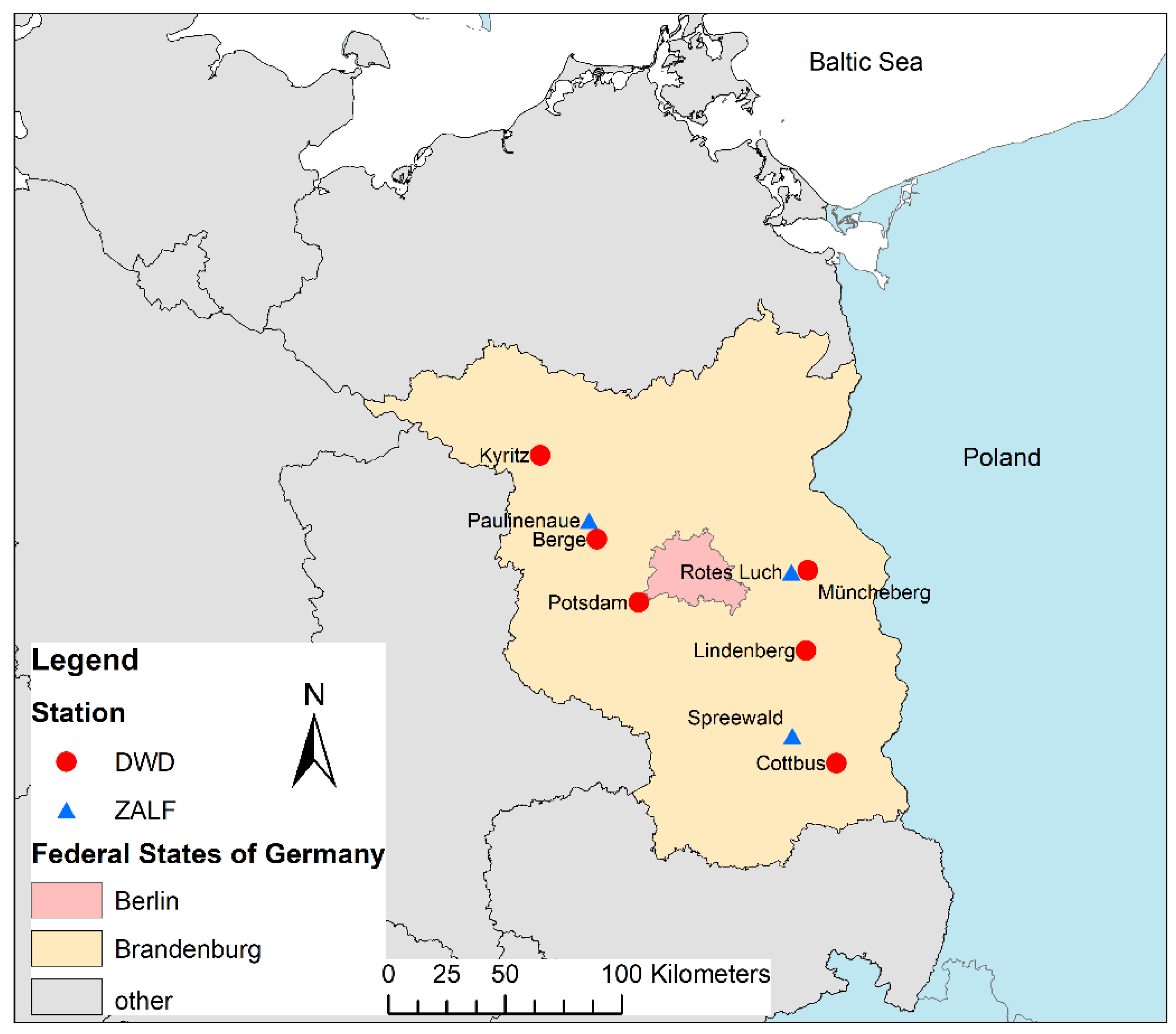
In this study, meteorological variables from WGSs in three regions (Märkische Schweiz, Spreewald, Havelland), in the federal state of Brandenburg (Germany), were compared with the values of neighbouring DWD stations (Figure 1, Table 1). Within the WGSs, our own measurements were carried out with standard automatic measurement stations (AMSs) from the Leibniz Centre for Agricultural Landscape Research (ZALF). The network of DWD stations enables a representative overview of climatic conditions in Germany to be compiled. The length of the measurement series ranges between a few decades to over 100 years. The locations of the measurement sites and the technical equipment meet the requirements of the WMO [56].
Since the term ‘microclimate’ is used in the literature cited in the paper to describe a relatively wide range of scales, we distinguish in the following between the local climate and the landscape climate. The local climate is at the location of a measuring station and the landscape climate is in the region considered here: Märkische Schweiz, Spreewald or Havelland.
The three study regions are all located in the area around Berlin. The DWD station, at Müncheberg, is located east of Berlin, in the Märkische Schweiz region. The ZALF measurement station, at the Rotes Luch fen site, was approximately 6.5 km from the DWD station in Müncheberg. Southeast of Berlin is the Spreewald region with the well-known wetland of the same name. The ZALF measurement station was located near the settlement of Burg, in the middle of the wetland. The nearest DWD measurement stations are Cottbus (22 km southeast of the WGS) and Lindenberg (38 km north of the WGS). To the west of Berlin, Havelländisches Luch extends into the Berlin Urstromtal (glacial valley), in the Havelland region. The WGS of the ZALF research station in Paulinenaue is located in the middle of the lowland area. The nearest DWD station is Berge, 8 km away, on the edge of the lowland. Southeast of the Havelland, there is the DWD station in Potsdam, 39 km away, and 35 km to the northwest, the DWD station in Kyritz.
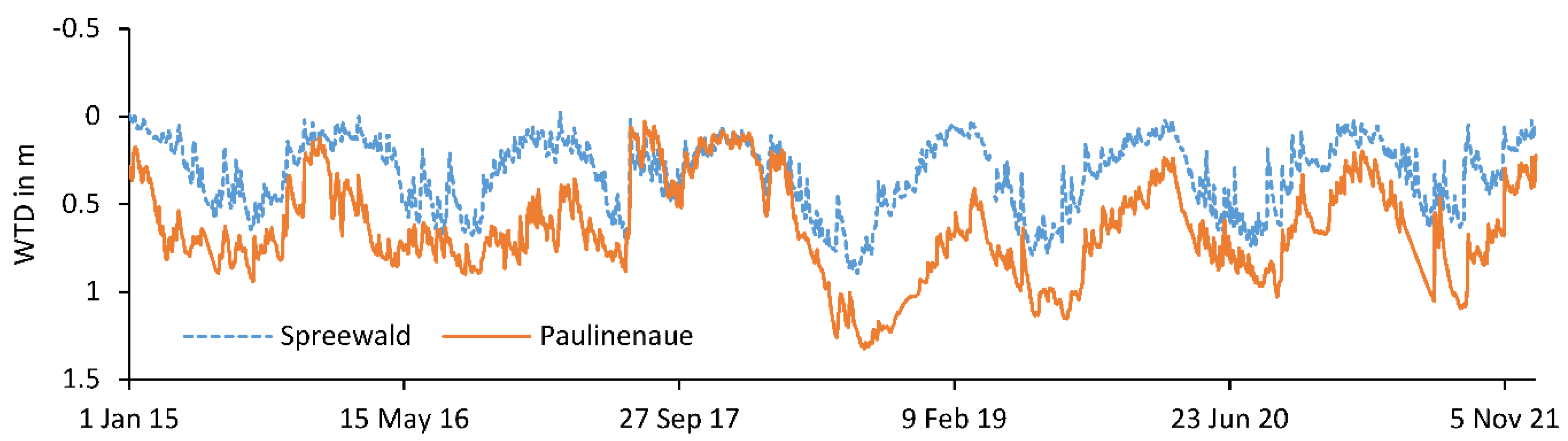
All three WGSs are drained fens that are used agriculturally as wet grassland. As a result of decades to centuries of drainage and agricultural use, the peatlands are severely degraded and only of low thickness. The WTDs vary from region to region. In the Spreewald, the study areas are often flooded in winter and spring (Figure 2). In the study period, they dropped to 0.5 m below ground level in summer in average years, and only in very dry years to a maximum of 0.9 m below ground level. In Rotes Luch, the WTDs on the study site fluctuated between the ground surface and a maximum of 1 m below ground level during the study period, from 2008 to 2011. The lowest WTDs were found on the sites in Paulinenaue. In average years, the summer WTDs were 0.9 m below ground level, and in extremely dry years they dropped to 1.3 m below ground level. In winter they were about 0.2 m below ground level. The different regional behaviour of the WTDs reflects their dependence on the water supply from the catchment area. While the areas in Rotes Luch and Paulinenaue are only supplied by a groundwater inflow from a relatively small catchment area, the Spreewald wetland has a comparably large catchment area: the Spree catchment area. In addition, mine water from the opencast lignite mines and water management reservoirs in the catchment area provide an additional water supply in dry periods, so that the WTDs can be better stabilised in summer [57].
2.2. Methods and Data
Hourly and daily values of Ta and VP gathered by the DWD from a total of six stations from 2008 to 2021 [58,59] were used along with our own measured values from two automatic measurement stations (AMS1, AMS2). The AMS1 station was used at various locations, and AMS2 exclusively in the Spreewald wetland. All DWD data are freely available in the Climate Data Center (CDC) of the DWD. The sensors used at the DWD stations are described in the CDC.
The AMS1 station uses a combined HMP45C sensor (Vaisala) to measure Ta and relative humidity at a height of 2 m. A CR3000 data logger (Campbell) records 15-min average values of Ta and VP. The sensor and logger are part of an eddy covariance station (Campbell). The AMS2 station is an automatic weather station. Ta and relative humidity at a height of 2 m are recorded using a combined PC-ME sensor (Galltec + mela). The values are measured at 1-min intervals and stored on a data logger (DL-104, UGT). All measured values are combined into hourly averages and daily averages. The values of the relative humidity (U in %) are converted into the VP by means of the VPD (both in kPa).
VPD results from the Magnus formula. According to Foken [60] for Ta > 0.01 °C.
and for Ta ≤ 0.01 °C. Ta is used in °C.
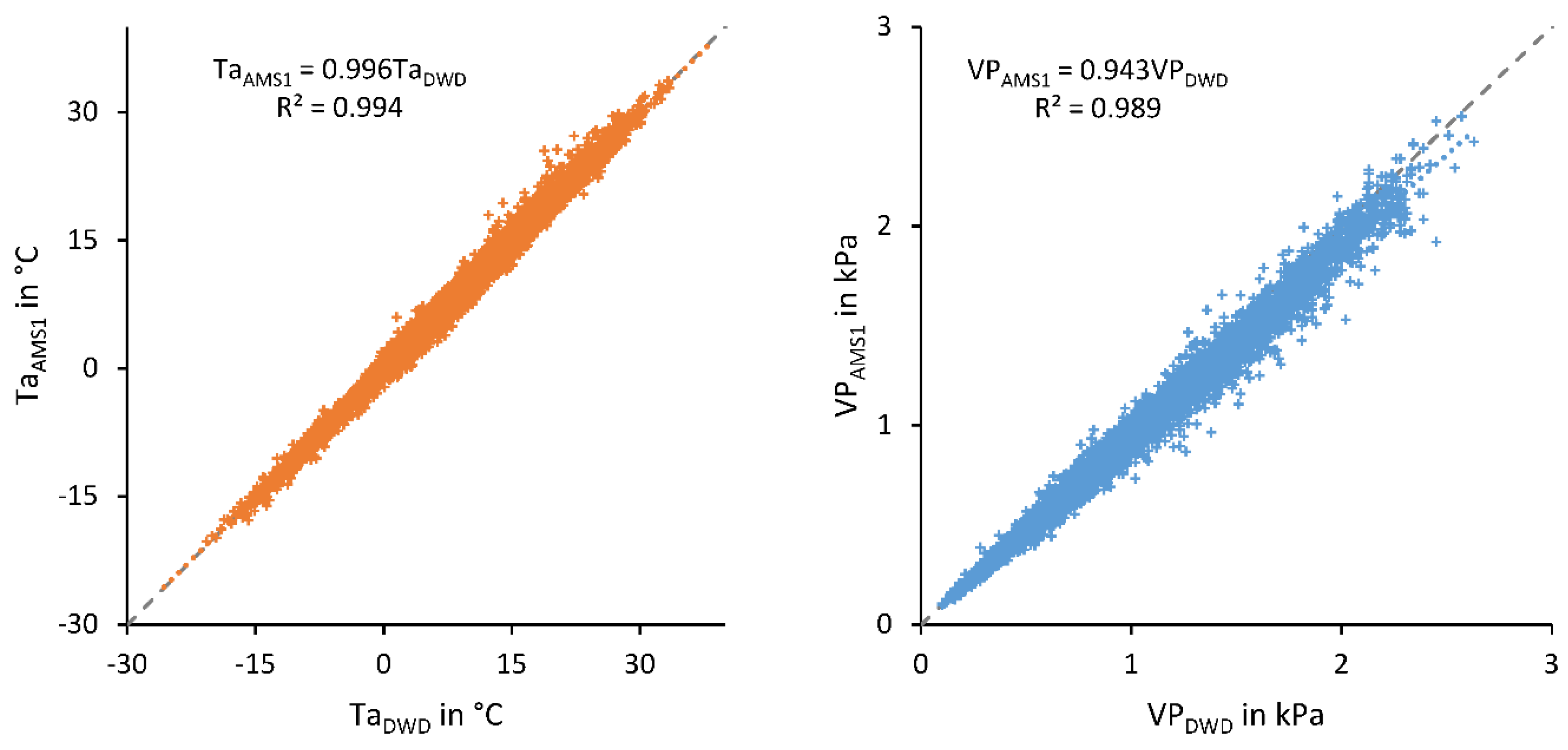
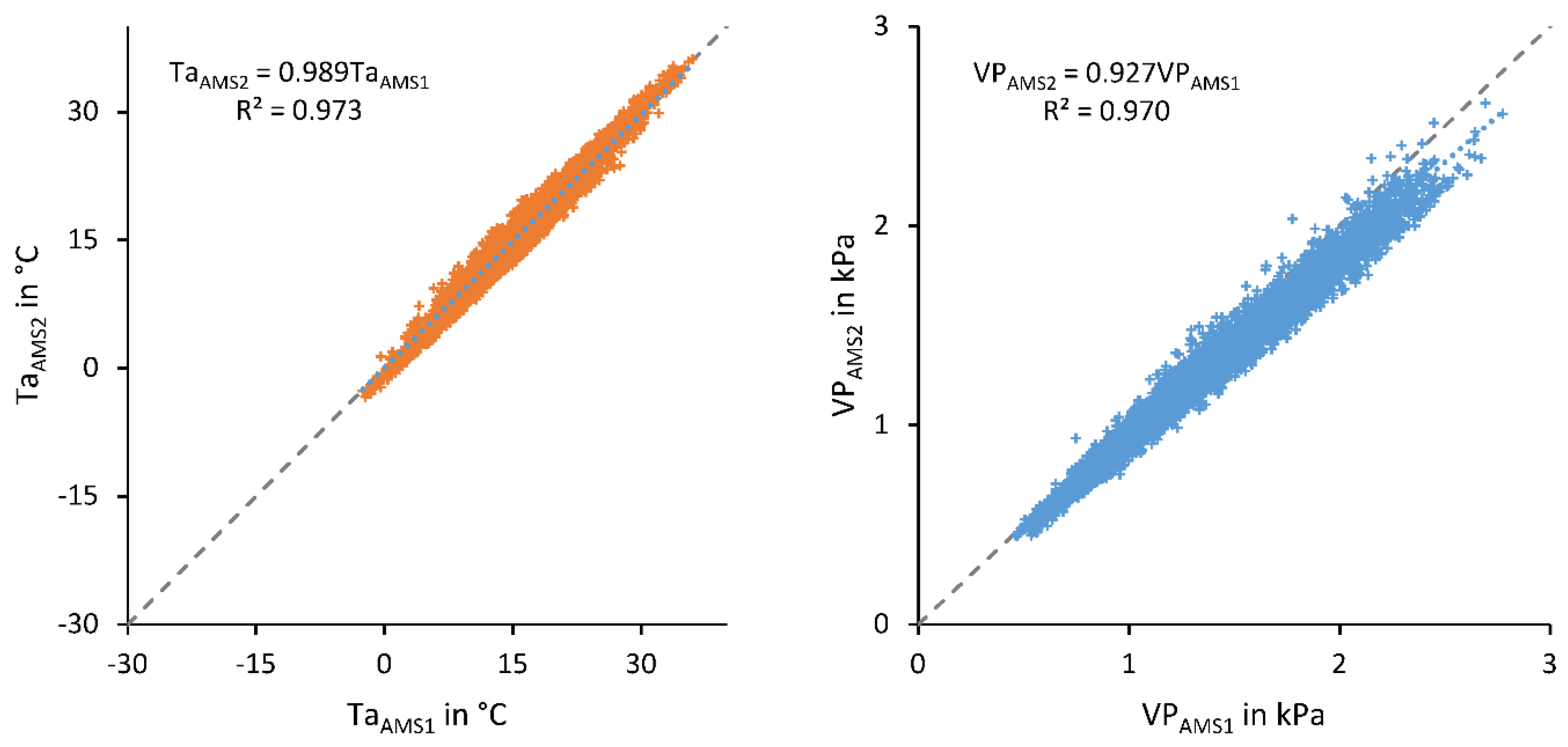
In order to exclude systematic measurement errors due to inaccurately calibrated sensors at the AMS, the measured Ta and VP values of AMS1 were compared with the measured values of the DWD station at the Müncheberg site. The sensors of DWD stations are regularly checked and can therefore serve as a reference. Only days with at least 22 hourly values were selected. At the Spreewald site, the Ta and VP of AMS1 and AMS2 were compared (Table 2).
The AMS1 station was used at various locations from 2008 to 2014 (Müncheberg, Rotes Luch, Spreewald) and continuously in Paulinenaue from 2015. As a result, the comparison periods have different lengths in these regions. Table 2 provides an overview of the scope of data and the time periods used for comparisons in the three regions.
All three WGSs were equipped with transects of groundwater observation wells with automatic data logger systems. The data on one well in the centre of each site was selected to characterise the WTD of the site. The data were collected in 15-min intervals on the data logger and summarised to average daily values during post-processing.
2.3. Sensor Comparison
Criteria for the comparison of the measured values are, following Foken [60], the root mean square error (RMSE), the bias (bias) and the precision (s). The RMSE, bias and s are calculated as follows for the example of Ta
First, the hourly average Ta and VP values of the AMS1 station and the DWD station Müncheberg were compared. For this purpose, the AMS1 station at the Müncheberg site was set up in an open field at a distance of approximately 50 m from the DWD station. To correct the AMS1 values, simple linear correction functions were derived (Equations (7) and (8)) and applied.
In the period from 2012 to 2014, the comparisons were carried out in the same way for the AMS1 and AMS2 stations at the Spreewald site. The AMS1 and AMS2 stations were set up approximately 5 m apart for this purpose.
All further evaluations were performed with the corrected values from stations AMS1 and AMS2.
2.4. Comparison by Location
The comparison of the Ta and VP of an AMS in a WGS and the nearest DWD station outside the WGS was based on the daily average values. For each of the three regions of Spreewald, Havelland and Märkische Schweiz, the time period given in Table 1 was taken as a basis and the values were compared. The length of the period was limited by the respective time an AMS was installed in the WGS. The measured values for the Spreewald region and the Havelland region were each summarised for different periods: the entire year; the winter half-year (October to March); the summer half-year (April to September) and the summer months (June to August). For better comparability, the period for the Spreewald was limited to the period from 1 January 2015 to 31 December 2021. In Märkische Schweiz, only the daily values were compared, as the measurement series is too short and does not cover all the months of a year. The significance of the deviations was examined using a T-test. The Kolmogorov–Smirnov test was used to verify the normal distribution.
Using the hourly average values, the average diurnal cycles and their deviations between the WGSs and the nearest DWD sites were compared for the three regions.
3. Results
3.1. Sensor Comparisons
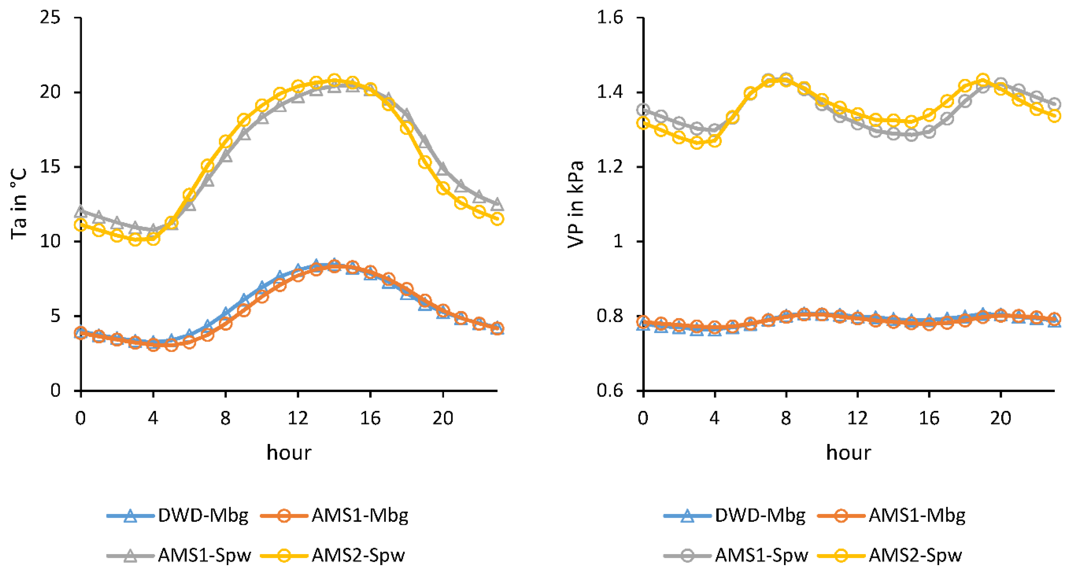
The comparisons of the measured Ta at the Müncheberg site (AMS1–DWD, Figure 3) and at the Spreewald site (AMS2–AMS1, Figure 4) both show a low scatter and a good agreement of the measured values. By applying the correction functions (Equations (7) and (9)), the quality criteria were slightly improved once again (Table 3). The relatively small deviations at the Müncheberg site are partly due to the longer comparison period and the larger range of measured values. The average diurnal variations of the Ta in the comparison periods also agree well (Figure 5).
On the other hand, when the VP of the AMS1 station is compared with the DWD station in Müncheberg (Figure 3), and the AMS1 station is compared with the AMS2 station at the WGS in the Spreewald wetland (Figure 4), this reveals a systematic deviation for both sensor comparisons (Figure 3 and Figure 4). The application of the correction functions (Equations (8) and (10)) reduces the deviations significantly (Table 3). The RMSE decreases at the Müncheberg site from 0.066 kPa to 0.046 kPa and at the Spreewald site from 0.118 kPa to 0.064 kPa. The somewhat larger scatter of the measured values in Figure 4 compared to Figure 3 is partly related to the comparison periods. The AMS1 station was set up more frequently in the winter months at the Müncheberg site, and in the summer months at the Spreewald site, which is also shown by the mean daily variations in the Ta (Figure 5). In summer, the VP values reach higher values overall and have a greater daily amplitude, with two characteristic maxima in the early morning and late afternoon. The greater dynamics of the values leads to greater deviations between the sensors. The average diurnal variations of the VP in Figure 5 underline this once more. All further comparisons use the VP values corrected according to Equations (8) and (10).
3.2. Ta Comparison by Location
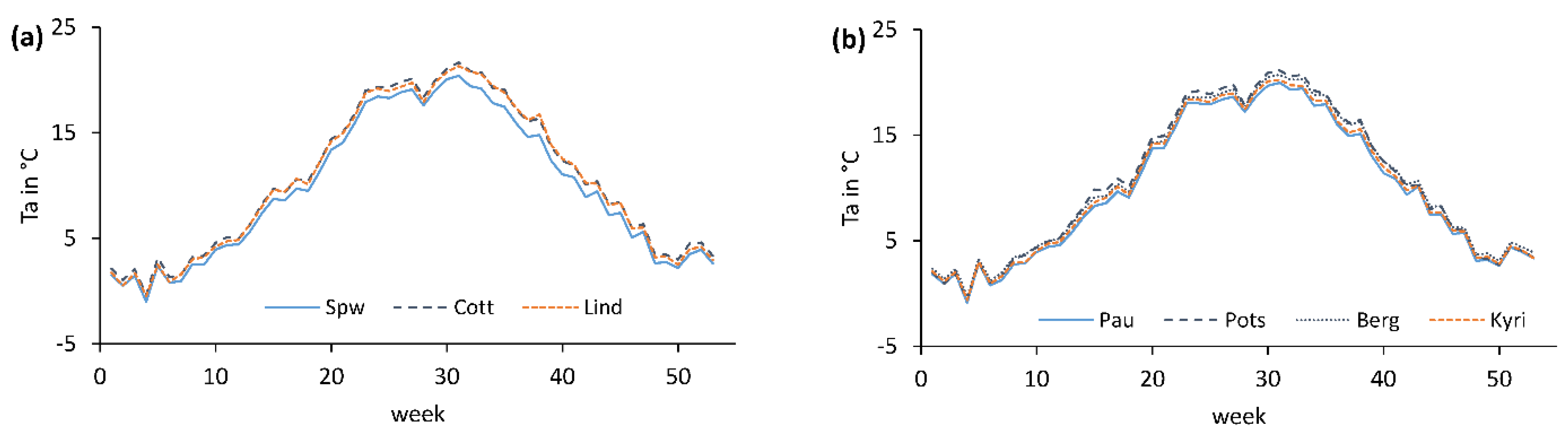
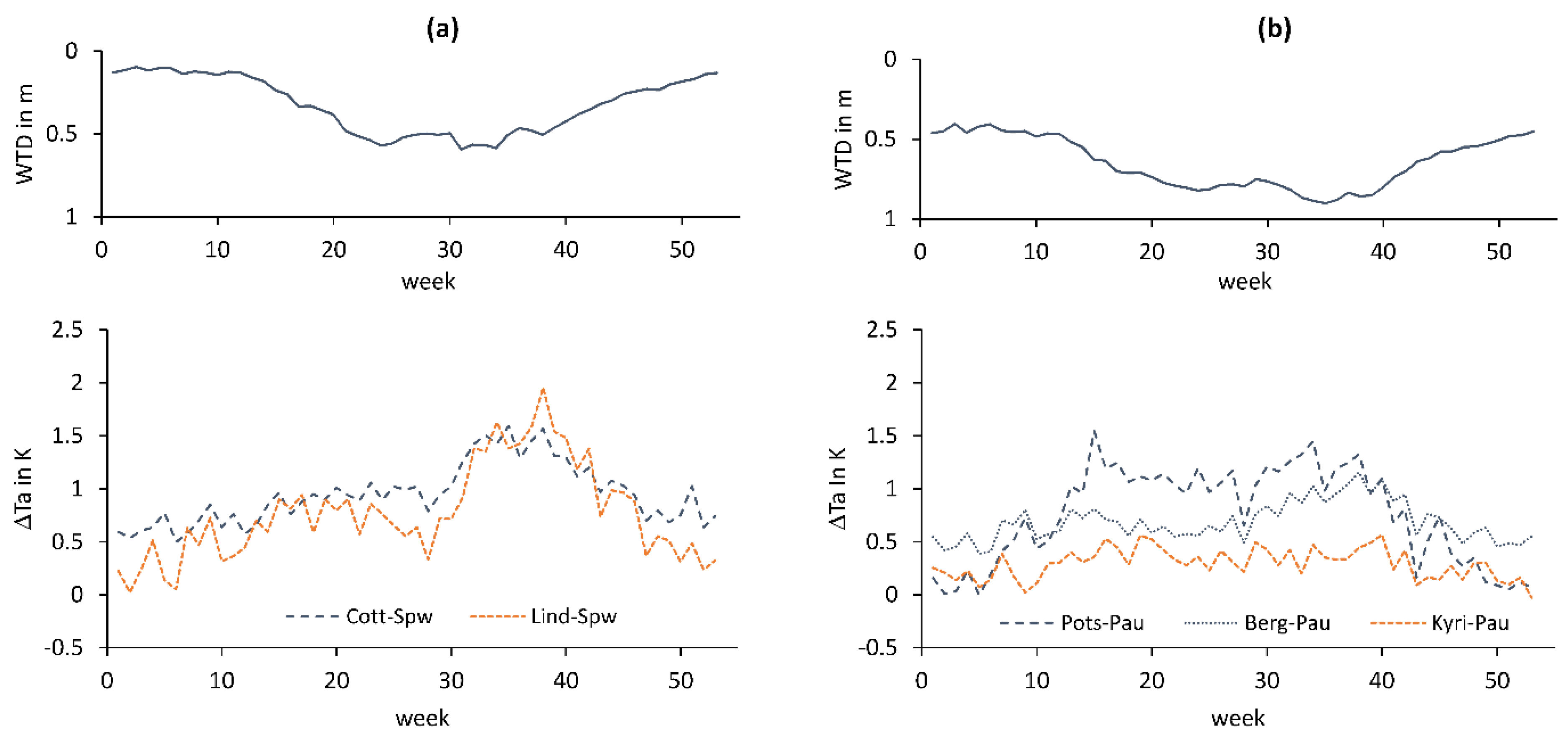
The annual cycle of the Ta at a height of 2 m shows the same pattern in the Spreewald and Havelland regions (Figure 6). Individual characteristic peaks or decreases in the average Ta curve are identical in both regions. The evaluation of the measured Ta shows a lower average weekly Ta in the WGSs in both regions compared to their neighbouring DWD stations (Figure 6). This is more evident in the summer half-year, with higher Ta, than in the winter half-year. The deviation of the Spreewald values from the values of the DWD station Cottbus is always highly significant (p < 0.001, Table 4). The deviation from the Lindenberg station is highly significant with the exception of the winter half-year. There are no significant differences between the northern Lindenberg station and the southern Cottbus station. Figure 7a shows that the difference between Cottbus and Spreewald is only slightly greater than the difference between Lindenberg and Spreewald. The annual cycle is identical. Between the 30th and 45th weeks, the differences increase to 1.5 K, while in winter they are less than 1 K.
The temperatures in Paulinenaue are highly significantly lower than in Berge and Potsdam for the whole year, the summer half-year and the summer months (p < 0.001, Table 4). Between Paulinenaue and the more westerly station in Kyritz, the deviations are only weakly significant in the summer half-year and the summer months (p < 0.05, Table 4). Between the DWD stations located outside the lowlands in Havelland there are also differences for individual evaluation periods at varying levels of significance. In particular, the station in Kyritz has lower temperatures compared to Berge and Potsdam, which means that the average Ta difference between Kyritz and the station in Paulinenaue does not exceed 0.5 K (Figure 7b).
For the Märkische Schweiz region there is only a comparison for the summer half-year and the summer months, as there were significantly fewer measurements in the years from 2008 to 2011 (Table 2). A calculation of the complete annual variation is not possible due to the small amount of data. The Ta on the WGS of Rotes Luch were significantly lower than outside the lowland in Müncheberg (Table 4).
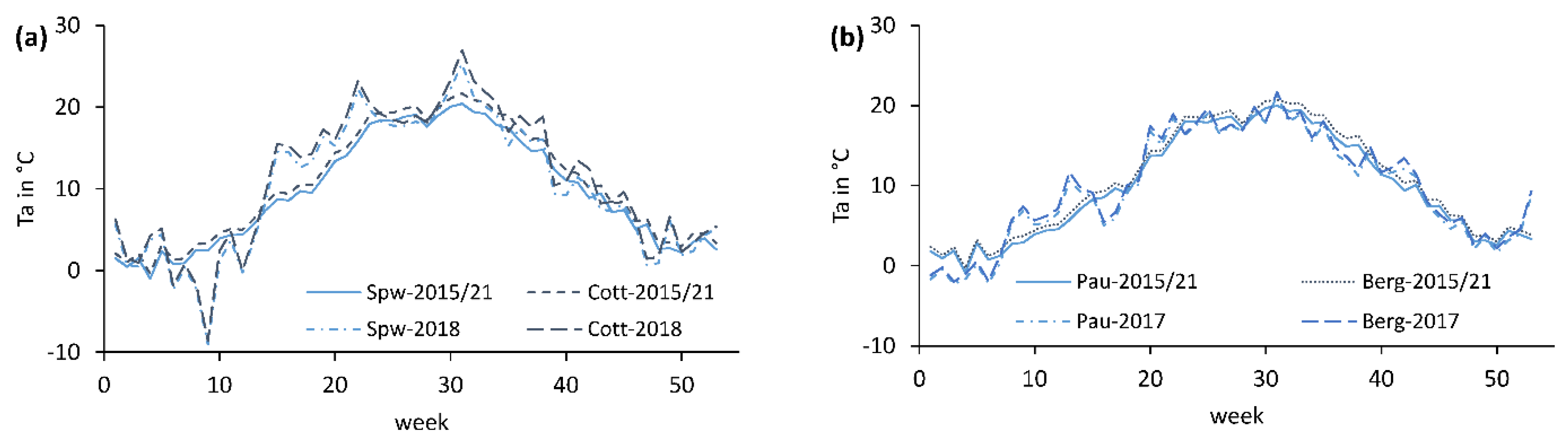
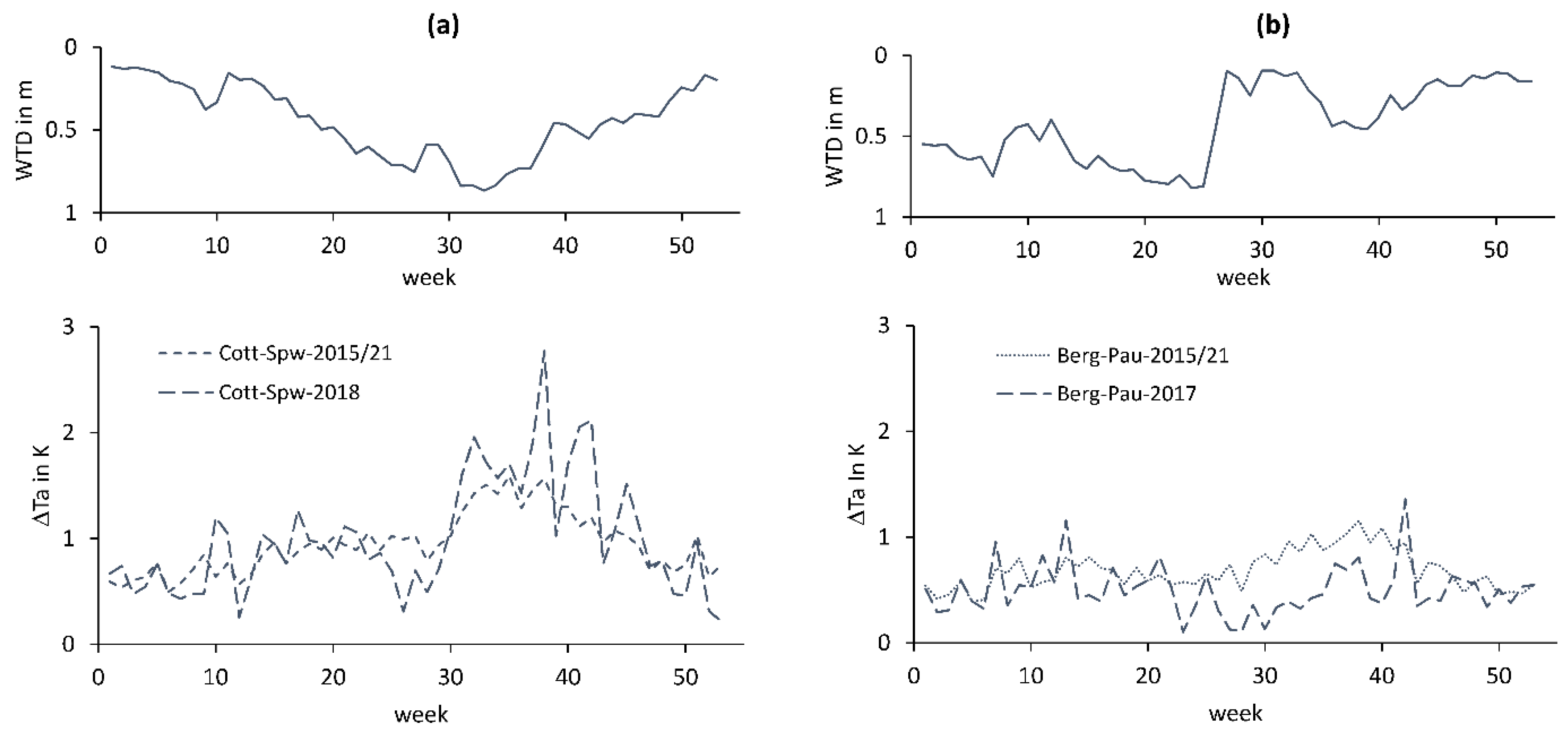
In addition to the weekly average values for the period 2015 to 2021, the dry year of 2018 is considered for the Spreewald region and the extremely wet year of 2017 for Havelland region. The annual variation in the Ta shows frequent above-average temperatures in the Spreewald region in 2018 for the period from the 15th to the 35th week (Figure 8a). The differences between the Spreewald wetland and the surrounding area change little during this period compared to the average values (Figure 9a). Only from the 35th week are they above the average values. The WTDs at the measurement site in the Spreewald wetland also drop deeper than in the other years (Figure 2).
The comparison of the Ta in the wet year of 2017, in contrast to Paulinenaue and the neighbouring Berge, with the average values from 2015 to 2021, shows only minor deviations in the annual cycle (Figure 8b). There is no sign that the significant increase in the groundwater table at the WGS in Paulinenaue at the end of June 2017 (Figure 2) affected the Ta. The temperature difference between the WGS and the neighbouring Berge station decreases from around 1 K to around 0.5 K compared to the mean trend (Figure 9b).
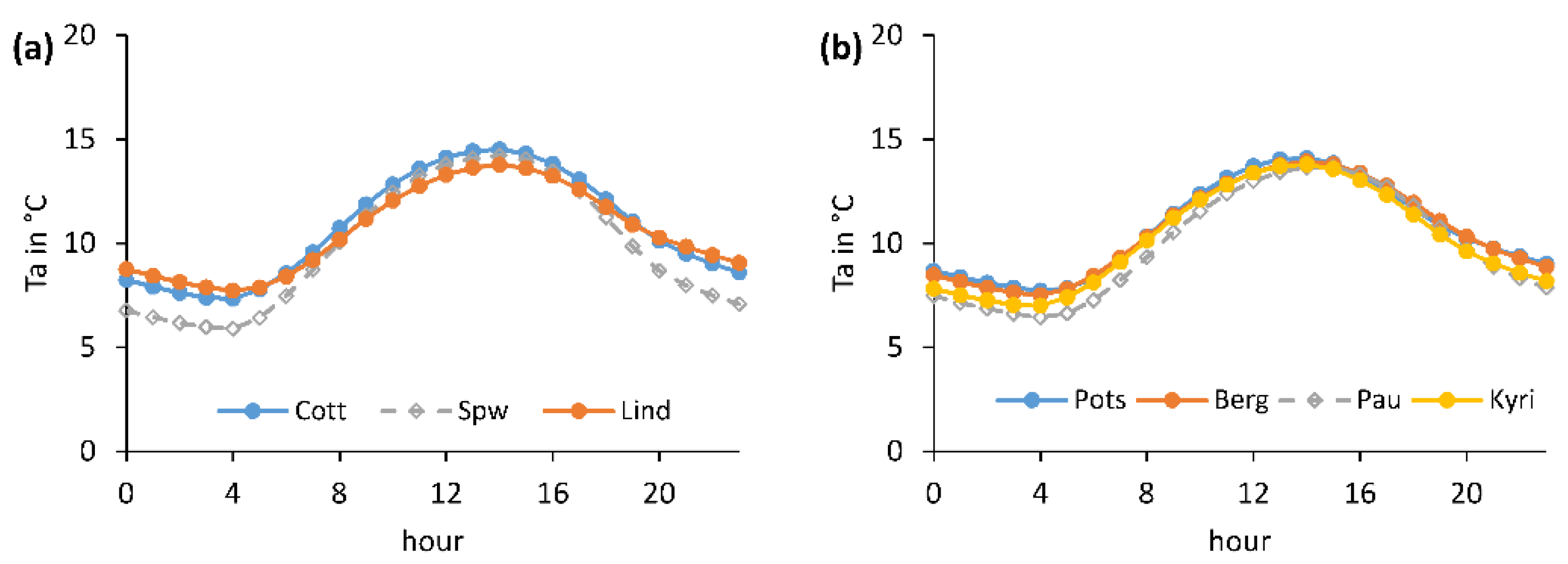
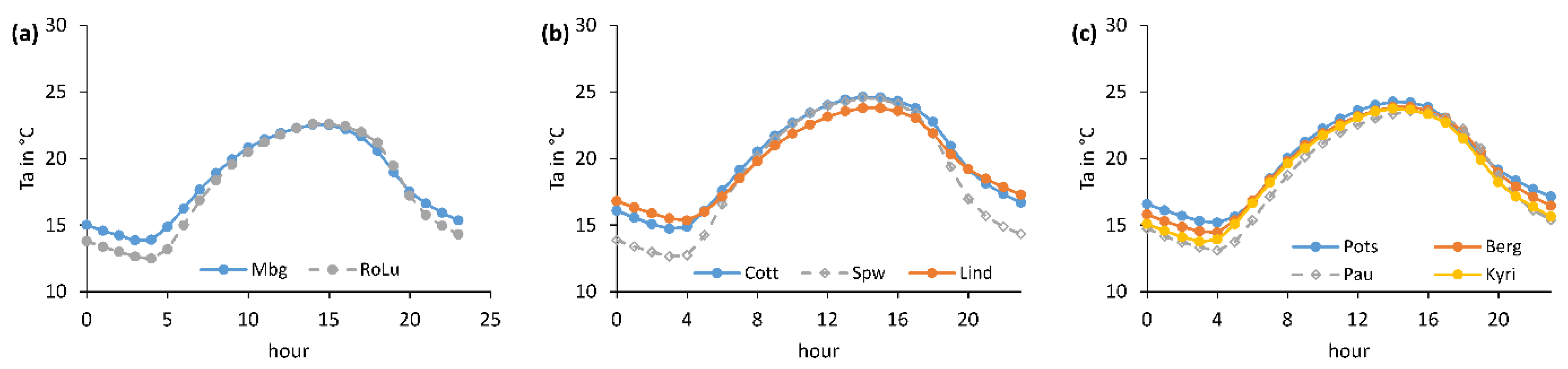
The average diurnal cycles of Ta at a height of 2 m shows a comparable diurnal cycle in all three regions and for all evaluation periods and the same behaviour when comparing the WGS and the neighbouring DWD station (Figure 10, Figure 11, Figure 12 and Figure 13). At night, the temperatures in the WGSs are always significantly cooler than outside the lowlands. During the day, the differences decrease, and towards the middle of the day the temperatures are at the same level. The different daily average temperatures in Table 4 are therefore particularly caused by temperature differences during the night hours.
3.3. VP Comparison by Location
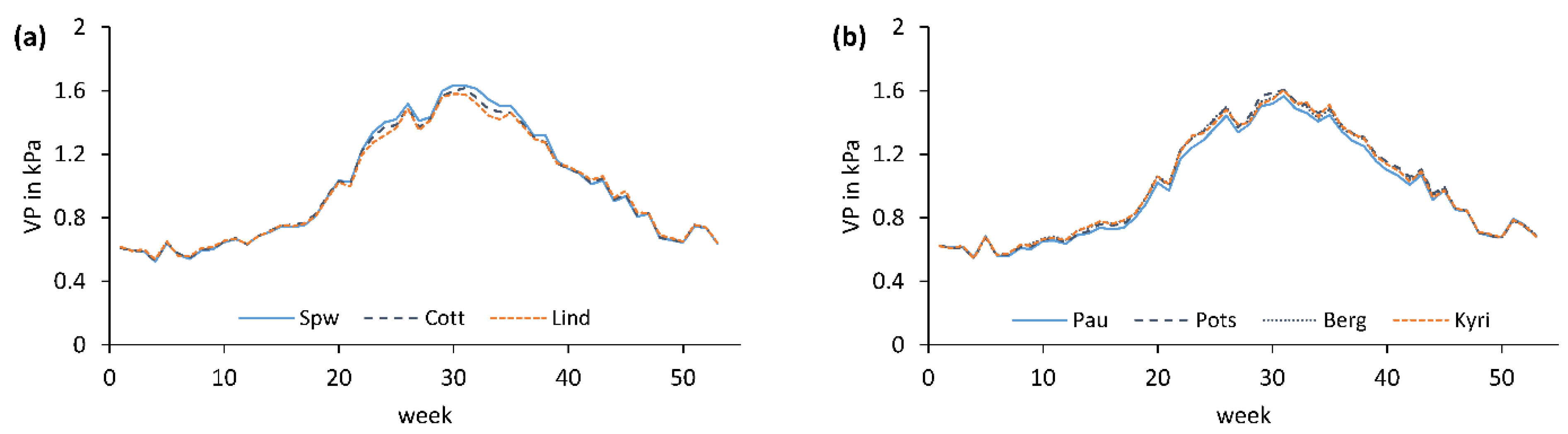
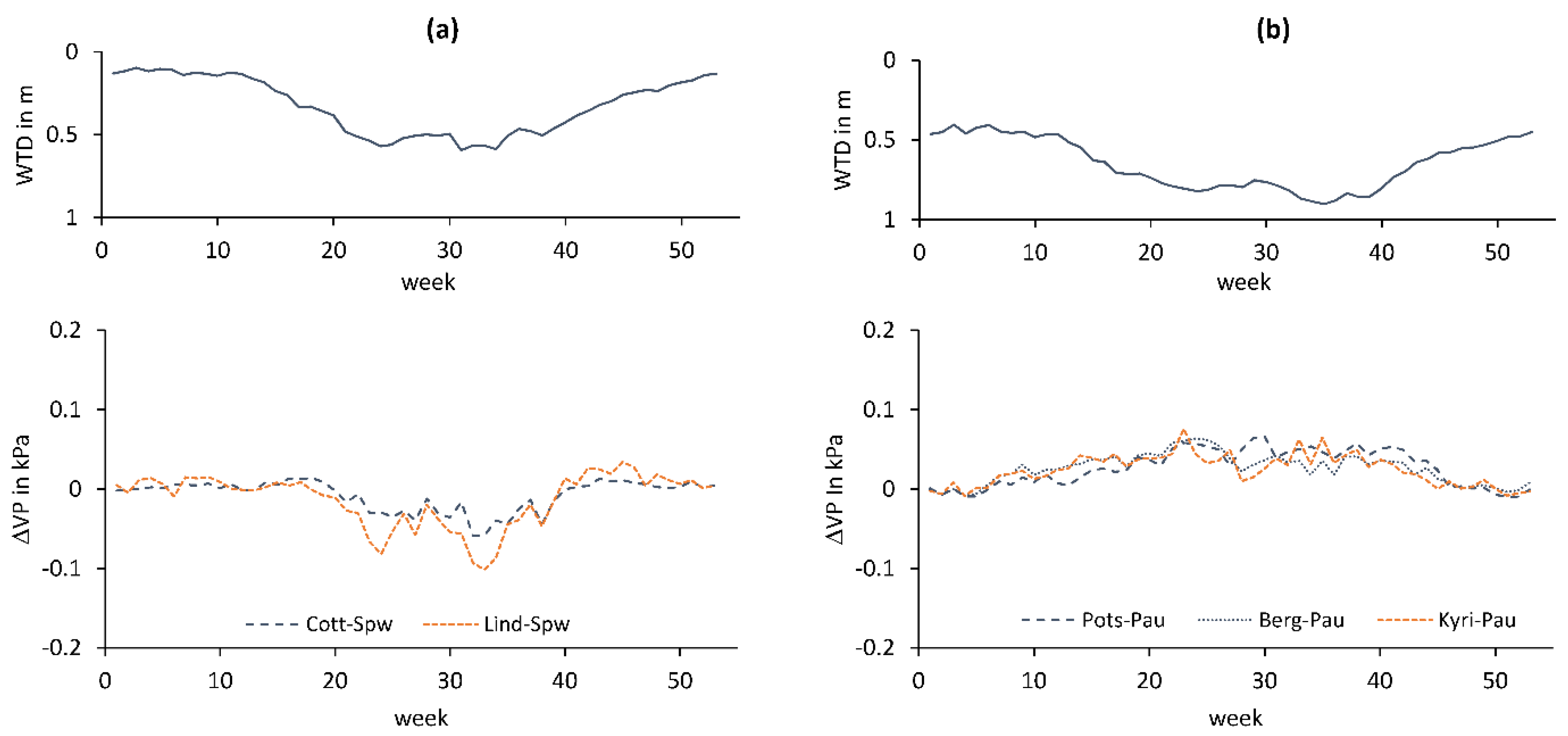
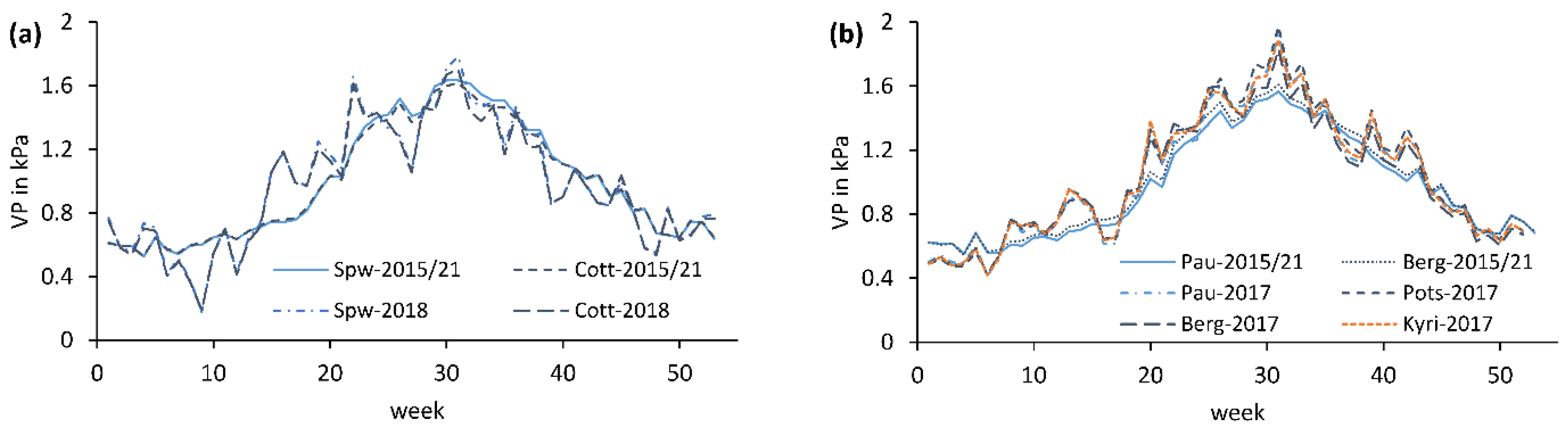
The average annual cycle of the VP shows an almost identical pattern for both regions, with marked deviations in the same calendar weeks (Figure 14). This underlines the fact that the average annual cycle of the VP, similarly to the annual cycle of the Ta, is largely determined by the transregional meteorological conditions that are reflected in both regions. However, there are differences when the VPs in the WGSs are compared with those at the respective neighbouring stations. In Spreewald, the VP in the WGS is slightly higher (approximately 0.05 kPa) from the 20th to the 40th weeks than outside the WGS (Figure 15a). There are no significant differences during the rest of the year (Table 5). In Havelland, the situation is reversed. In the summer half-year, the VP in the WGS is significantly lower than outside it (Figure 15b, Table 5).
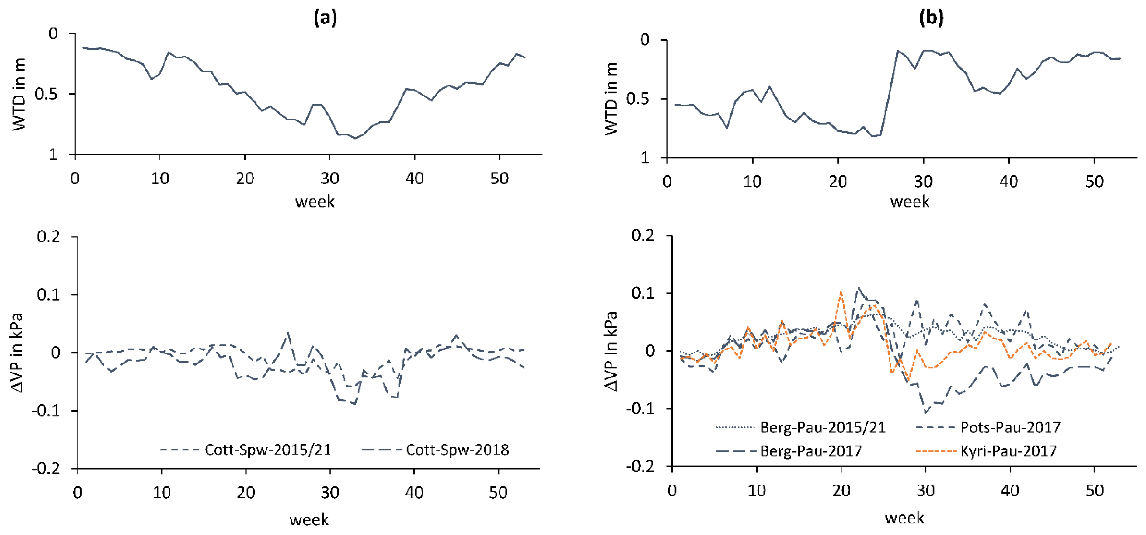
In the first half of the extremely dry year of 2018, the VPs measured in the WGSs and outside the lowlands are above the average values. In the second half of the year, they are often lower than the average values (Figure 16a). The differences between the WGSs and surrounding areas change only slightly (Figure 17a). It is only between the 30th and 40th week, the time with the lowest groundwater level at the measurement site in the Spreewald (Figure 2b), that the difference in VP increases from around −0.05 to −0.08 kPa between the WGS and the surrounding area.
In the wet year of 2017, with the significantly higher water levels compared to the average water levels at the Paulinenaue site (Figure 2), effects on the measured VPs are also more evident. The VP values in 2017 are above the average values of the years 2015–2021 almost the entire year, which can be seen particularly clearly after the 27th week (Figure 16b). Until the heavy precipitation at the end of June and the subsequent increase in the groundwater level, the VP values in Berge are still higher than at the WGS in Paulinenaue. Afterwards, the signs reverse from the 27th week (Figure 17b). The values at the WGS now exceed the values outside the lowland by up to 0.1 kPa. The reaction to the changed site conditions is more pronounced for the VP than for the Ta.
The comparison of the daily average values in Table 5 shows less significant differences overall between the values in the WGS and its surroundings for the VP than for the Ta. For the Märkische Schweiz region, no significant differences between Rotes Luch and the Müncheberg station are detectable.
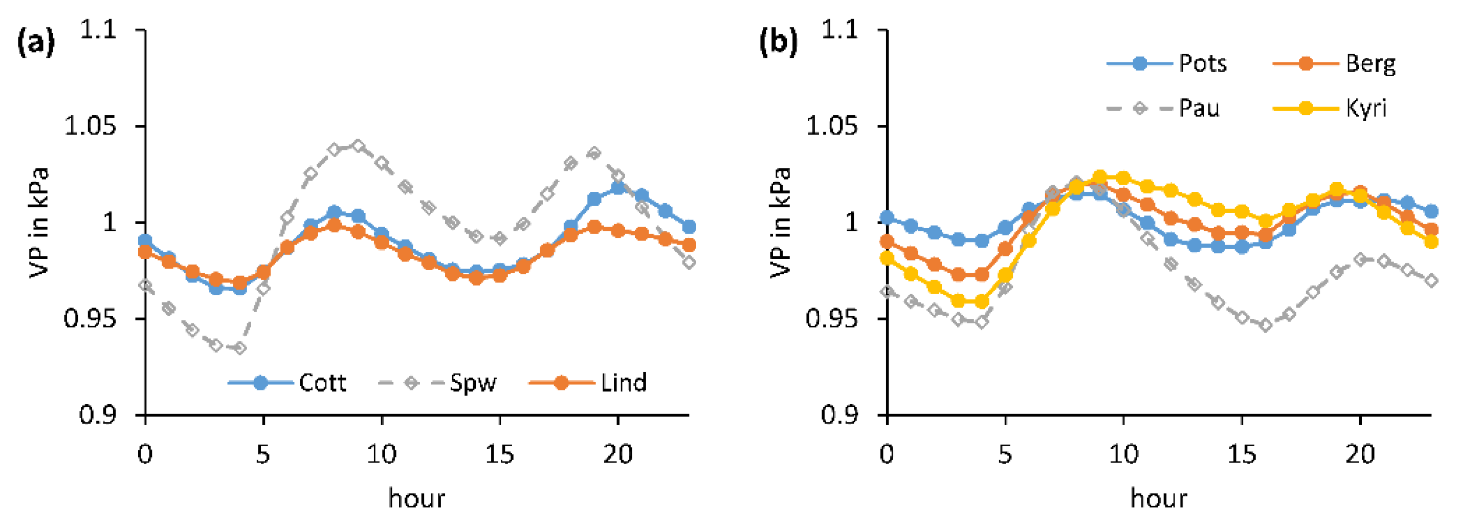
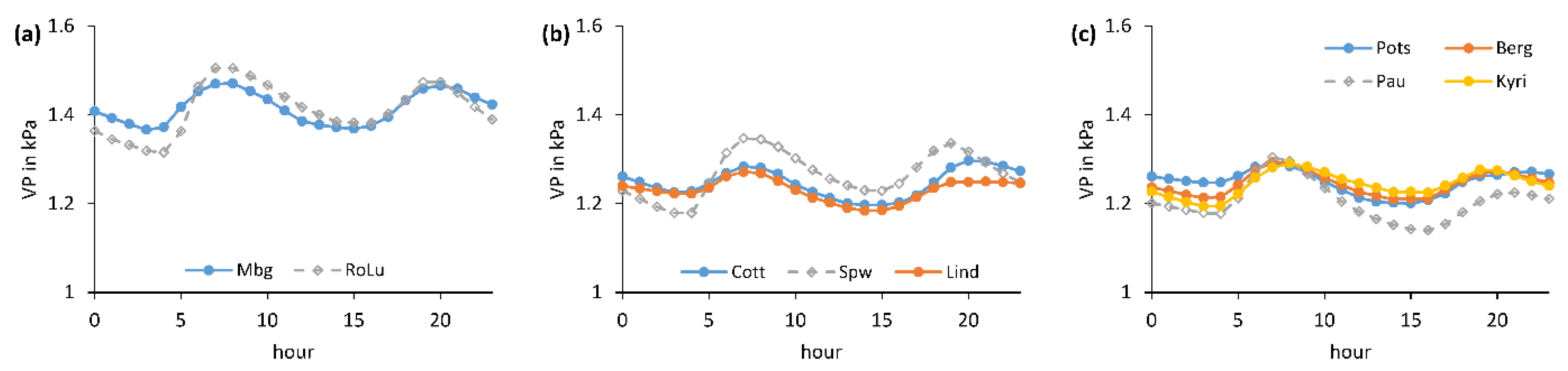
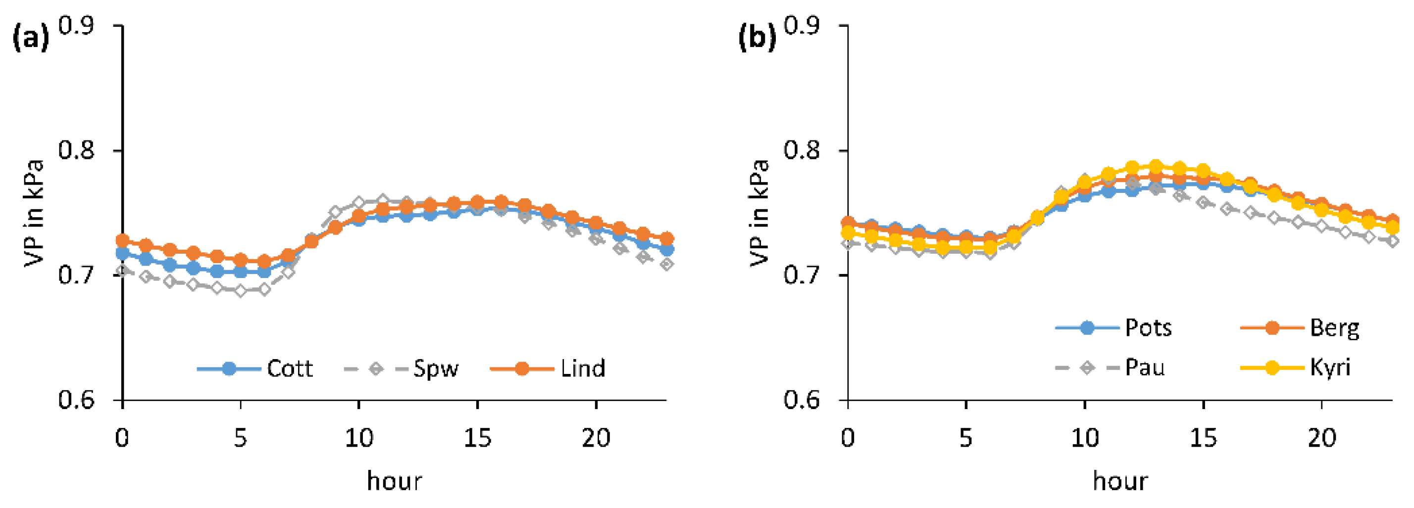
The average diurnal cycles for the whole year (Figure 18), and for different parts of the year (Figure 19, Figure 20 and Figure 21), underline the behaviour in the annual cycle. The diurnal cycle has the typical two maxima in the morning and in the late afternoon. In the Spreewald wetland, the values during the day are always higher than in the surrounding area. At night they are lower. In the Havelland region, the values in the WGS are lower than in the surrounding area throughout the day. The diurnal cycles of the stations in the Märkische Schweiz region are similar to those in the other two regions (Figure 19 and Figure 21). The differences between the WGS and the neighbouring station are somewhat less pronounced than in the Spreewald region, but more pronounced than in the Havelland region.
4. Discussion
Sensor comparison is necessary to minimise systematic errors and, in some cases, to detect very small differences between sites. The DWD stations are regularly checked, and if necessary recalibrated. Their values can therefore serve as a reference value for other stations, if they are set up at the same location. The results of the comparison confirm the need to correct the measured values from stations AMS1 and AMS2. For the measured Ta, the measured values agreed relatively well. However, correcting the measured values from stations AMS1 and AMS2 still reduced the differences. The measured VP values from stations AMS1 and AMS2 both had a more significant systematic deviation from the respective reference values (Figure 3 and Figure 4). They underline the need to check and correct the sensors and confirm the recommendation made by Foken [60]. The deviations were significantly reduced using simple linear correction functions (Table 2). After the corrections, there were no longer any significant differences in the mean values (p < 0.001). Kelvin, Acreman, Harding and Hess [32] had a similar problem in their investigations in England and were also able to correct it in this way. A regular check and recalibration of all the sensors at automatic weather stations, as recommended by WMO [56], among others, is therefore also recommended here.
The comparison of the Ta in WGSs with the nearest stations outside the lowlands shows significantly lower temperatures in the WGSs for all three regions of Märkische Schweiz, Spreewald and Havelland. In the summer months, the differences rise, at times, to 2 K. In the winter months, they are only 0.5 K in the Spreewald region and approach 0 K in the Havelland region. This corresponds to the descriptions in the literature of the cooler local climate in wetlands [34,39] and is one of many ecosystem services provided by wetlands [20,52,55]. However, the measured differences are relatively small; they average about 1 K per year (Table 4). This corresponds to the deviation of up to 1 K deviation the Ta in the fen and an outside station, recorded by Kelvin, Acreman, Harding and Hess [32], in measurements taken over a two-year period in England, but is significantly less than those reported by Hemes, Eichelmann, Chamberlain, Knox, Oikawa, Sturtevant, Verfaillie, Szutu and Baldocchi [30]. They found up to 5.1 K cooler daily Ta in restored fen sites in California compared to drained agricultural land. This shows the importance of the respective site conditions and the difficulties in generalising and transferring the results to other sites.
It is important to correctly classify the magnitudes of the measured Ta differences. For example, the Ta differences between the WGSs and the surrounding areas correspond to the Ta differences that the northwest-southeast climate gradient in the federal state of Brandenburg also exhibits. The comparison of the temperature difference between the WGS in Paulinenaue and the Havelland surroundings illustrates this. The DWD station Kyritz is located approximately 35 km northwest of the measuring site Paulinenaue, and the station Potsdam, 39 km southeast (Figure 1). The difference in average Ta between Potsdam and Kyritz is greater than the Ta difference between the WGS in Paulinenaue and the station in Kyritz. The effect of the transregional climatic conditions in western Brandenburg and the site-specific features together exceeds the climatic effect of the WGS in Paulinenaue. The Lindenberg and Cottbus stations are located approximately 38 km north and 22 km south-east of the WGS in the Spreewald region, respectively. In the north-south gradient, the transregional influence is less pronounced, and the climatic wetland effect is also stronger. This is due partly to the significantly wetter site conditions in the Spreewald wetland, but also to the weaker north-south gradient compared to the stronger west-east gradient in the transregional climate within Brandenburg.
Dietrich, Behrendt and Wegehenkel [48] found a significant increase in the average annual Ta of 1.1 K in Potsdam and Cottbus when comparing the 1961/1990 30-year series with 1991/2020. The measured annual Ta difference between the WGS in the Spreewald wetland and Cottbus is 0.9 K, and that between Potsdam and the WGS in Paulinenaue is 0.8 K (Table 4). This relates the measured differences in the regions studied to the climatic changes taking place over the last 30 years.
In extremely dry or wet years, the Ta of the sites considered sometimes show a different behaviour than perhaps expected. The year 2018 was warmer and drier than average in the study region. As a result, the water levels in the Spreewald wetland dropped significantly lower than average. It would be expected that the local climatic effect of the WGS would decrease due to the lower groundwater levels and that the Ta difference to the surrounding area would decrease. However, the temperature differences in the second half of 2018 (Figure 9a) show a larger Ta difference than on average. This proves the overall greater stability of the climatic conditions in the Spreewald wetland, compared to the surrounding area, despite the groundwater levels being lower than in normal years. The extreme weather conditions led to disproportionately higher temperatures in the surrounding area and, consequently, to greater temperature differences compared to the WGS.
The wet year of 2017 in the Havelland region was similar. High precipitation at the end of June led to a strong rise in the water table up to the ground surface. Large areas of land were inundated. This condition lasted for several weeks. One would expect a stronger cooling effect in the WGS and, consequently, an increase in the temperature difference compared to the surrounding area. However, a decrease in the temperature difference was measured (Figure 9b). Again, the effect of the wet weather on the surrounding, largely sandy sites was greater than the effect on the Ta of the WGS. It also underlines the greater stability of the climatic conditions in the WGS.
The question of this study is: what are the reasons for the lower temperatures in the WGSs? The term “evaporative cooling” is often used in this context. However, the comparison of the average diurnal cycles of the Ta for different periods of the year (Figure 10, Figure 11, Figure 12 and Figure 13) contradicts the thesis that an increased latent heat flux (or: ET) and reduced sensible heat flux leads to lower temperatures. In this case, Ta differences would have to occur in the daily period with ET. This is not the case in all periods of the year or in all study regions. The temperature differences occur during the night hours, when ET has no significance. This conclusion was also reached by Kelvin, Acreman, Harding and Hess [32] in their measurements in England and Słowińska, Słowiński, Marcisz and Lamentowicz [34] in Poland. Huryna, Brom and Pokorny [20], on the other hand, explain the temperature differences between WGSs and neighbouring agricultural areas exclusively with the higher ET. We cannot confirm this with our results. Conversely, however, it cannot be concluded that the ET in the WGSs is not higher than in the surrounding area. It is only true that it does not necessarily lead to lower Ta during the day. However, there are also studies that come to the opposite conclusion. Hemes, Eichelmann, Chamberlain, Knox, Oikawa, Sturtevant, Verfaillie, Szutu and Baldocchi [30] or Worrall, Howden, Burt, Rico-Ramirez and Kohler [40] found cooler Ta in restored wetland areas compared to neighbouring agricultural areas during the day, and warmer Ta at night. This is another indication of the importance of specific site conditions.
The lower night-time temperatures, which are mainly responsible for the lower daily average values, are a clear indication of the greater importance of the ground heat flux for the local climate at shallow groundwater sites [36]. Wet, organic soils, in particular, have a large heat storage capacity compared to dry, mineral soils. They can absorb and store more heat during the day and release it much more slowly. This leads to the differences shown in the diurnal cycle, but can also be seen in the annual soil temperature cycle. These soils warm up more slowly in spring and cool down more slowly in autumn. The shallow groundwater tables additionally influence these effects, as the groundwater is a large heat reservoir and provides for the high-water content of the soil. The soils of this location are warmed less at depth, but also cool less deeply. The importance of ground heat flux on wet sites was equally emphasised by Souch, Grimmond and Wolfe [22], however, they also pointed out that this makes the transferability of results difficult, as the results are always very site-specific.
The average annual cycle of the VP in the Spreewald and Havelland regions is almost identical. Marked ups and downs occur equally in both regions and confirm the effect of the transregional meteorological conditions. The comparison of the VP of the WGSs and the surrounding area shows differences between the values. However, these are only significant in summer and amount to about 0.05 kPa on average. In the winter half-year, the differences are not significant.
In the two regions of Spreewald and Havelland, the signs of the differences between the WGSs and the respective surrounding area differ. All DWD stations outside the WGSs (Potsdam, Berge, Kyritz, Cottbus and Lindenberg) have comparable mean values between 1.23 kPa and 1.25 kPa in the summer half-year, and 1.45 kPa and 1.47 kPa in the three summer months (Table 5). The corresponding values of the WGS in the Spreewald wetland are above the values of the surrounding area (1.27 kPa and 1.51 kPa), and those of the WGS in Paulinenaue are below the surrounding area values (1.20 kPa and 1.42 kPa). Not all differences are significant (Table 5). The opposite signs of the differences are due to the different ET at the two WGSs. The Spreewald wetland has a relatively large catchment area and is therefore relatively well supplied with water even in the summer months. As a result, water levels drop less deeply, and the ET of the site is not limited by water availability. Large parts of the area are forested and have a high ET even in summer. This leads to comparatively higher water contents in the air. The lowland site around Paulinenaue, on the other hand, has a relatively small catchment area and is therefore largely dependent only on precipitation. There are no significant inflows. As a result, the groundwater levels in summer drop significantly lower than in the Spreewald wetland and water availability may be limited, meaning that the ET is also reduced. Worrall, Boothroyd, Howden, Burt, Kohler and Gregg [33] also found that the ET of a wetland site does not necessarily have to be high. They justify the lower VP values in a restored bog area in England compared to the surrounding countryside with the lower ET in the special shrub vegetation in the bog area.
The VP values of the two extreme years of 2017 and 2018 underline this. In the wet year of 2017, water availability was no longer limited after the high precipitation and the associated increase in groundwater levels in Paulinenaue. Some of the grass stands could no longer be harvested. Lush grass stands led to high ET. As a result, the VP values show the same behaviour as in the Spreewald wetland. They exceed the values of the surrounding area by up to 0.1 kPa. In the year 2018, which was dryer and warmer than average, the overall VP values are below the average values from 2015 to 2021, and the difference between the WGS and the surrounding area increases even more, although the WGS values are also below the average values. This shows that the area surrounding the Spreewald wetland was more affected by the dry, hot conditions than the WGS itself.
In contrast to the diurnal cycles of the Ta, the diurnal cycles of the VP show differences in the night-time and day-time hours. Higher VP values during the day in the Spreewald wetland compared to the surrounding area are the result of high ET. Lower VP values in Paulinenaue compared to the surrounding area and also compared to the Spreewald WGS indicate lower ET compared to the surrounding area (Figure 18). At the same time, the surrounding area values in the Havelland region are somewhat higher than in the area surrounding the Spreewald wetland. The lower VP values at night are a consequence of the increased dew formation in the WGSs, which in turn stems from the lower night-time temperatures. The values from the third study region, Märkische Schweiz, confirm the statements from the other two regions, but are less meaningful due to the short data series.
5. Conclusions
The results and findings show that the WGSs studied have similar special local climatic conditions to wetlands, compared to their surrounding areas. They show that there are significant differences and special features in the local climate of the WGSs, but that these are relatively small. This underlines the demanding requirements that have to be met, in terms of the accuracy and length of the measurement series for the meteorological variables, in order to be able to draw reliable conclusions on the climatic effect of WGSs.
The reason for the cooler Ta of the WGSs is not only a higher ET, but also the greater heat storage potential of the moist, organic soil with its balancing effect. This is clearly demonstrated by the diurnal cycles of the Ta of the WGSs compared to the surrounding area: they are only lower than in the surrounding area during the night hours. A precise quantification of the ground heat flux and soil heat storage in and outside WGSs would explain the observed temperature differences even better. This would also allow more precise estimates of how climatic or hydrological changes affect the heat balance of WGSs, and of WGSs’ potential as possible cool oases in an increasingly warming environment.
A more humid local climate in the WGSs could not be clearly verified. While the Spreewald wetland is wetter in summer than the surrounding area, this does not apply unreservedly at the Paulinenaue site. In the winter half-year, no significant differences were detectable between the WGSs and the surrounding area. The frequently higher relative humidity in these areas is mainly due to the influence of temperature when calculating the vapour pressure deficit (Equations (2) and (3)).
Whether the restoration of the WGS, which is associated with higher water levels and possibly an even higher ET, increases the meteorological differences cannot be directly deduced from the available results. This would require a detailed investigation of appropriate sites. Further micrometeorological investigations, in particular, should also include direct measurements of ET and ground heat flux in order to better understand the relevant processes.
Author Contributions
O.D. processed and analyzed the data, wrote the original draft, and designed the tables and figures. A.B. performed the measurements in Paulinenaue and gave important input to the manuscript. All authors have read and agreed to the published version of the manuscript.
Funding
The APC was funded by the Leibniz Open Access Publishing Fund.
Acknowledgments
We would like to thank our colleague Mario Weipert for supervising the weather station, the eddy covariance station and the groundwater level measurements. We also thank the technical staff of the Experimental Station in Paulinenaue for their support.
Conflicts of Interest
The authors declare no conflict of interest.
References
- Bechtold, M.; Tiemeyer, B.; Laggner, A.; Leppelt, T.; Frahm, E.; Belting, S. Large-scale regionalization of water table depth in peatlands optimized for greenhouse gas emission upscaling. Hydrol. Earth Syst. Sci. 2014, 18, 3319–3339. [Google Scholar] [CrossRef] [Green Version]
- Tiemeyer, B.; Albiac Borraz, E.; Augustin, J.; Bechtold, M.; Beetz, S.; Beyer, C.; Drösler, M.; Ebli, M.; Eickenscheidt, T.; Fiedler, S.; et al. High emissions of greenhouse gases from grasslands on peat and other organic soils. Glob. Change Biol. 2016, 22, 4134–4149. [Google Scholar] [CrossRef] [PubMed]
- Drösler, M.; Freibauer, A.; Christensen, T.R.; Friborg, T. Observations and Status of Peatland Greenhouse Gas Emissions in Europe. In The Continental-Scale Greenhouse Gas Balance of Europe; Dolman, A.J., Valentini, R., Freibauer, A., Eds.; Springer: New York, NY, USA, 2008; pp. 243–261. [Google Scholar] [CrossRef]
- Tiemeyer, B.; Freibauer, A.; Borraz, E.A.; Augustin, J.; Bechtold, M.; Beetz, S.; Beyer, C.; Ebli, M.; Eickenscheidt, T.; Fiedler, S.; et al. A new methodology for organic soils in national greenhouse gas inventories: Data synthesis, derivation and application. Ecol. Indic. 2020, 109, 105838. [Google Scholar] [CrossRef]
- BMUV. Nationale Moorschutzstrategie (in German, National Peat Protection Strategy.); Bundesministerium für Umwelt, Naturschutz, Nukleare Sicherheit und Verbraucherschutz: Berlin, Germany, 2021; p. 54. [Google Scholar]
- Hesslerová, P.; Pokorný, J.; Huryna, H.; Harper, D. Wetlands and Forests Regulate Climate via Evapotranspiration. In Wetlands: Ecosystem Services, Restoration and Wise Use; An, S., Verhoeven, J.T.A., Eds.; Springer International Publishing: Cham, Switzerland, 2019; pp. 63–93. [Google Scholar] [CrossRef]
- Helbig, M.; Waddington, J.M.; Alekseychik, P.; Amiro, B.D.; Aurela, M.; Barr, A.G.; Black, T.A.; Blanken, P.D.; Carey, S.K.; Chen, J.; et al. Increasing contribution of peatlands to boreal evapotranspiration in a warming climate. Nat. Clim. Change 2020, 10, 555–560. [Google Scholar] [CrossRef]
- Lafleur, P.M.; Rouse, W.R. The Influence of Surface Cover and Climate on Energy Partitioning and Evaporation in A Subarctic Wetland. Bound.-Layer Meteorol. 1988, 44, 327–347. [Google Scholar] [CrossRef]
- Lafleur, P.M. Evapotranspiration from Sedge-Dominated Wetland Surfaces. Aquat. Bot. 1990, 37, 341–353. [Google Scholar] [CrossRef]
- Lafleur, P.M.; Roulet, N.T. A Comparison of Evaporation Rates from 2 Fens of the Hudson-Bay Lowland. Aquat. Bot. 1992, 44, 59–69. [Google Scholar] [CrossRef]
- Campbell, D.I.; Williamson, J.L. Evaporation from a raised peat bog. J. Hydrol. 1997, 193, 142–160. [Google Scholar] [CrossRef]
- Burba, G.G.; Verma, S.B.; Kim, J. Energy fluxes of an open water area in a mid-latitude prairie wetland. Bound.-Layer Meteorol. 1999, 91, 495–504. [Google Scholar] [CrossRef]
- Burba, G.G.; Verma, S.B.; Kim, J. A comparative study of surface energy fluxes of three communities (Phragmites australis, Scirpus acutus, and open water) in a prairie wetland ecosystem. Wetlands 1999, 19, 451–457. [Google Scholar] [CrossRef]
- Burba, G.G.; Verma, S.B.; Kim, J. Surface energy fluxes of Phragmites australis in a prairie wetland. Agric. For. Meteorol. 1999, 94, 31–51. [Google Scholar] [CrossRef]
- Thompson, M.A.; Campbell, D.I.; Spronken-Smith, R.A. Evaporation from natural and modified raised peat bogs in New Zealand. Agric. For. Meteorol. 1999, 95, 85–98. [Google Scholar] [CrossRef]
- Eaton, A.K.; Rouse, W.R.; Lafleur, P.M.; Marsh, P.; Blanken, P.D. Surface energy balance of the western and central Canadian subarctic: Variations in the energy balance among five major terrain types. J. Clim. 2001, 14, 3692–3703. [Google Scholar] [CrossRef]
- Kellner, E. Surface energy fluxes and control of evapotranspiration from a Swedish Sphagnum mire. Agric. For. Meteorol. 2001, 110, 101–123. [Google Scholar] [CrossRef]
- Gavin, H.; Agnew, C.A. Modelling actual, reference and equilibrium evaporation from a temperate wet grassland. Hydrol. Process. 2004, 18, 229–246. [Google Scholar] [CrossRef]
- Peacock, C.E.; Hess, T.M. Estimating evapotranspiration from a reed bed using the Bowen ratio energy balance method. Hydrol. Process. 2004, 18, 247–260. [Google Scholar] [CrossRef]
- Huryna, H.; Brom, J.; Pokorny, J. The importance of wetlands in the energy balance of an agricultural landscape. Wetl. Ecol. Manag. 2014, 22, 363–381. [Google Scholar] [CrossRef]
- Price, J.S. Hydrology and microclimate of a partly restored cutover bog, Quebec. Hydrol. Process. 1996, 10, 1263–1272. [Google Scholar] [CrossRef]
- Souch, C.; Grimmond, C.S.B.; Wolfe, C.P. Evapotranspiration rates from wetlands with different disturbance histories: Indiana Dunes National Lakeshore. Wetlands 1998, 18, 216–229. [Google Scholar]
- Jacobs, J.M.; Mergelsberg, S.L.; Lopera, A.F.; Myers, D.A. Evapotranspiration from a wet prairie wetland under drought conditions: Paynes Prairie Preserve, Florida, USA. Wetlands 2002, 22, 374–385. [Google Scholar] [CrossRef]
- Lafleur, P.M.; Hember, R.A.; Admiral, S.W.; Roulet, N.T. Annual and seasonal variability in evapotranspiration and water table at a shrub-covered bog in southern Ontario, Canada. Hydrol. Process. 2005, 19, 3533–3550. [Google Scholar] [CrossRef]
- Gasca-Tucker, D.L.; Acreman, M.C.; Agnew, C.T.; Thompson, J.R. Estimating evaporation from a wet grassland. Hydrol. Earth Syst. Sci. 2007, 11, 270–282. [Google Scholar] [CrossRef]
- Sottocornola, M.; Kiely, G. Energy fluxes and evaporation mechanisms in an Atlantic blanket bog in southwestern Ireland. Water Resour. Res. 2010, 46, 1–13. [Google Scholar] [CrossRef] [Green Version]
- Zhang, Q.; Sun, R.; Jiang, G.; Xu, Z.; Liu, S. Carbon and energy flux from a Phragmites australis wetland in Zhangye oasis-desert area, China. Agric. For. Meteorol. 2016, 230–231, 45–57. [Google Scholar] [CrossRef]
- Acreman, M.C.; Harding, R.J.; Lloyd, C.R.; McNeil, D.D. Evaporation characteristics of wetlands: Experience from a wet grassland and a reedbed using eddy correlation measurements. Hydrol. Earth Syst. Sci. 2003, 7, 11–21. [Google Scholar] [CrossRef] [Green Version]
- Siedlecki, M.; Pawlak, W.; Fortuniak, K.; Zielinski, M. Wetland Evapotranspiration: Eddy Covariance Measurement in the Biebrza Valley, Poland. Wetlands 2016, 36, 1055–1067. [Google Scholar] [CrossRef] [Green Version]
- Hemes, K.S.; Eichelmann, E.; Chamberlain, S.D.; Knox, S.H.; Oikawa, P.Y.; Sturtevant, C.; Verfaillie, J.; Szutu, D.; Baldocchi, D.D. A Unique Combination of Aerodynamic and Surface Properties Contribute to Surface Cooling in Restored Wetlands of the Sacramento-San Joaquin Delta, California. J. Geophys. Res. Biogeosciences 2018, 123, 2072–2090. [Google Scholar] [CrossRef]
- Raney, P.A.; Fridley, J.D.; Leopold, D.J. Characterizing Microclimate and Plant Community Variation in Wetlands. Wetlands 2014, 34, 43–53. [Google Scholar] [CrossRef]
- Kelvin, J.; Acreman, M.C.; Harding, R.J.; Hess, T.M. Micro-climate influence on reference evapotranspiration estimates in wetlands. Hydrol. Sci. J. 2017, 62, 378–388. [Google Scholar] [CrossRef]
- Worrall, F.; Boothroyd, I.M.; Howden, N.J.K.; Burt, T.P.; Kohler, T.; Gregg, R. Are peatlands cool humid islands in a landscape? Hydrol. Process. 2020, 34, 5013–5025. [Google Scholar] [CrossRef]
- Słowińska, S.; Słowiński, M.; Marcisz, K.; Lamentowicz, M. Long-term microclimate study of a peatland in Central Europe to understand microrefugia. Int. J. Biometeorol. 2022, 66, 817–832. [Google Scholar] [CrossRef] [PubMed]
- Philippov, D.A.; Yurchenko, V.V. Data on air temperature, relative humidity and dew point in a boreal Sphagnum bog and an upland site (Shichengskoe mire system, North-Western Russia). Data Brief 2019, 25, 104156. [Google Scholar] [CrossRef]
- Fernández-Pascual, E.; Correia-Álvarez, E. Mire microclimate: Groundwater buffers temperature in waterlogged versus dry soils. Int. J. Climatol. 2021, 41, E2949–E2958. [Google Scholar] [CrossRef]
- Aalto, J.; Tyystjärvi, V.; Niittynen, P.; Kemppinen, J.; Rissanen, T.; Gregow, H.; Luoto, M. Microclimate temperature variations from boreal forests to the tundra. Agric. For. Meteorol. 2022, 323, 109037. [Google Scholar] [CrossRef]
- Wu, Y.; Xi, Y.; Feng, M.; Peng, S. Wetlands Cool Land Surface Temperature in Tropical Regions but Warm in Boreal Regions. Remote Sens. 2021, 13, 1439. [Google Scholar] [CrossRef]
- Worrall, F.; Boothroyd, I.M.; Gardner, R.L.; Howden, N.J.K.; Burt, T.P.; Smith, R.; Mitchell, L.; Kohler, T.; Gregg, R. The Impact of Peatland Restoration on Local Climate: Restoration of a Cool Humid Island. J. Geophys. Res. Biogeosciences 2019, 124, 1696–1713. [Google Scholar] [CrossRef]
- Worrall, F.; Howden, N.J.K.; Burt, T.P.; Rico-Ramirez, M.A.; Kohler, T. Local climate impacts from ongoing restoration of a peatland. Hydrol. Process. 2022, 36, e14496. [Google Scholar] [CrossRef]
- Helbig, M.; Wischnewski, K.; Kljun, N.; Chasmer, L.E.; Quinton, W.L.; Detto, M.; Sonnentag, O. Regional atmospheric cooling and wetting effect of permafrost thaw-induced boreal forest loss. Glob. Change Biol. 2016, 22, 4048–4066. [Google Scholar] [CrossRef] [Green Version]
- Helbig, M.; Waddington, J.M.; Alekseychik, P.; Amiro, B.; Aurela, M.; Barr, A.G.; Black, T.A.; Carey, S.K.; Chen, J.; Chi, J.; et al. The biophysical climate mitigation potential of boreal peatlands during the growing season. Environ. Res. Lett. 2020, 15, 104004. [Google Scholar] [CrossRef]
- Herbst, M.; Kappen, L. The ratio of transpiration versus evaporation in a reed belt as influenced by weather conditions. Aquat. Bot. 1999, 63, 113–125. [Google Scholar] [CrossRef]
- Drexler, J.Z.; Anderson, F.E.; Snyder, R.L. Evapotranspiration rates and crop coefficients for a restored marsh in the Sacramento-San Joaquin Delta, California, USA. Hydrol. Process. 2008, 22, 725–735. [Google Scholar] [CrossRef]
- Headley, T.R.; Davison, L.; Huett, D.O.; Muller, R. Evapotranspiration from subsurface horizontal flow wetlands planted with Phragmites australis in sub-tropical Australia. Water Res. 2012, 46, 345–354. [Google Scholar] [CrossRef] [PubMed]
- Anda, A.; Da Silva, J.A.T.; Soos, G. Evapotranspiration and crop coefficient of common reed at the surroundings of Lake Balaton, Hungary. Aquat. Bot. 2014, 116, 53–59. [Google Scholar] [CrossRef]
- Triana, F.; Di Nasso, N.N.O.; Ragaglini, G.; Roncucci, N.; Bonari, E. Evapotranspiration, crop coefficient and water use efficiency of giant reed (Arundo donax L.) and miscanthus (Miscanthusxgiganteus Greef et Deu.) in a Mediterranean environment. Glob. Change Biol. Bioenergy 2015, 7, 811–819. [Google Scholar] [CrossRef]
- Dietrich, O.; Behrendt, A.; Wegehenkel, M. The Water Balance of Wet Grassland Sites with Shallow Water Table Conditions in the North-Eastern German Lowlands in Extreme Dry and Wet Years. Water 2021, 13, 2259. [Google Scholar] [CrossRef]
- Queluz, J.G.T.; Pereira, F.F.S.; Sanchez-Roman, R.M. Evapotranspiration and crop coefficient for Typha latifolia in constructed wetlands. Water Qual. Res. J. Can. 2018, 53, 53–60. [Google Scholar] [CrossRef]
- Admiral, S.W.; Lafleur, P.M. Partitioning of latent heat flux at a northern peatland. Aquat. Bot. 2007, 86, 107–116. [Google Scholar] [CrossRef]
- Drexler, J.Z.; Snyder, R.L.; Spano, D.; Paw, K.T.U. A review of models and micrometeorological methods used to estimate wetland evapotranspiration. Hydrol. Process. 2004, 18, 2071–2101. [Google Scholar] [CrossRef]
- Acreman, M.C.; Harding, R.J.; Lloyd, C.; McNamara, N.P.; Mountford, J.O.; Mould, D.J.; Purse, B.V.; Heard, M.S.; Stratford, C.J.; Dury, S.J. Trade-off in ecosystem services of the Somerset Levels and Moors wetlands. Hydrol. Sci. J. 2011, 56, 1543–1565. [Google Scholar] [CrossRef]
- Hesslerová, P.; Pokorný, J.; Brom, J.; Rejšková—Procházková, A. Daily dynamics of radiation surface temperature of different land cover types in a temperate cultural landscape: Consequences for the local climate. Ecol. Eng. 2013, 54, 145–154. [Google Scholar] [CrossRef]
- Maclean, I.M.D.; Duffy, J.P.; Haesen, S.; Govaert, S.; De Frenne, P.; Vanneste, T.; Lenoir, J.; Lembrechts, J.J.; Rhodes, M.W.; Van Meerbeek, K. On the measurement of microclimate. Methods Ecol. Evol. 2021, 12, 1397–1410. [Google Scholar] [CrossRef]
- Huryna, H.; Pokorný, J. The role of water and vegetation in the distribution of solar energy and local climate: A review. Folia Geobot. 2016, 51, 191–208. [Google Scholar] [CrossRef]
- WMO. Guide to Instruments and Methods of Observation. Volume I—Measurement of Meteorological Variables; World Meteorological Organization: Geneva, Switzerland, 2018; pp. 1–573. [Google Scholar]
- Grünewald, U. Water resources management in river catchments influenced by lignite mining. Ecol. Eng. 2001, 17, 143–152. [Google Scholar] [CrossRef]
- DWD, C.D.C.C. Historical Daily Station Observations (Temperature, Pressure, Precipitation, Sunshine Duration, etc.) for Germany, Version v21.3, 2021. (DWD), D.W., Ed. Offenbach, 2022. Available online: https://opendata.dwd.de/climate_environment/CDC/observations_germany/climate/daily/ (accessed on 8 April 2022).
- DWD, C.D.C.C. Historical Hourly Station Observations of 2m Air Temperature and Humidity for Germany, Version v006, 2018. (DWD), D.W., Ed. Offenbach, 2022. Available online: https://opendata.dwd.de/climate_environment/CDC/observations_germany/climate/hourly/ (accessed on 8 April 2022).
- Foken, T. Micrometeorology; Springer: Berlin/Heidelberg, Germany, 2008; pp. 1–306. [Google Scholar]
Figure 1.
Location of the WGSs and DWD stations in the federal state of Brandenburg.

Figure 2.
Water table depths (WTDs) at the measurement sites in Spreewald and Paulinenaue for the years 2015 to 2021. In the Spreewald study site the average WTD was 0.33 m, in the Paulinenaue study site 0.65 m.
Figure 2.
Water table depths (WTDs) at the measurement sites in Spreewald and Paulinenaue for the years 2015 to 2021. In the Spreewald study site the average WTD was 0.33 m, in the Paulinenaue study site 0.65 m.

Figure 3.
Comparison of the measured hourly average values of air temperature (Ta) and vapour pressure (VP) of the AMS1 and DWD station at the Müncheberg site (Dataset 1 in Table 2).
Figure 3.
Comparison of the measured hourly average values of air temperature (Ta) and vapour pressure (VP) of the AMS1 and DWD station at the Müncheberg site (Dataset 1 in Table 2).

Figure 4.
Comparison of the measured hourly average values for the air temperature (Ta) and vapour pressure (VP) of the AMS1 and AMS2 station at the Spreewald site (Dataset 2 in Table 2).
Figure 4.
Comparison of the measured hourly average values for the air temperature (Ta) and vapour pressure (VP) of the AMS1 and AMS2 station at the Spreewald site (Dataset 2 in Table 2).

Figure 5.
Average diurnal cycle of the corrected air temperature (Ta) and the corrected vapour pressure (VP) during sensor comparison at the Müncheberg and Spreewald sites (datasets 1 and 2, Table 2).
Figure 5.
Average diurnal cycle of the corrected air temperature (Ta) and the corrected vapour pressure (VP) during sensor comparison at the Müncheberg and Spreewald sites (datasets 1 and 2, Table 2).

Figure 6.
Weekly average air temperature (Ta) at 2 m height in the regions Spreewald (a) and Havelland (b) for the years 2015 to 2021.
Figure 6.
Weekly average air temperature (Ta) at 2 m height in the regions Spreewald (a) and Havelland (b) for the years 2015 to 2021.

Figure 7.
Average water table depth (WTD) and difference in air temperature (Ta) at a height of 2 m comparing the WGSs in the lowlands and the neighbouring DWD stations outside the lowlands in the regions of Spreewald (a) and Havelland (b), weekly average values for 2015 to 2021.
Figure 7.
Average water table depth (WTD) and difference in air temperature (Ta) at a height of 2 m comparing the WGSs in the lowlands and the neighbouring DWD stations outside the lowlands in the regions of Spreewald (a) and Havelland (b), weekly average values for 2015 to 2021.

Figure 8.
Weekly average air temperature (Ta) at 2 m height in comparison with the average values for the years 2015 to 2021, (a): Spreewald region (2018), (b): Havelland region (2017).
Figure 8.
Weekly average air temperature (Ta) at 2 m height in comparison with the average values for the years 2015 to 2021, (a): Spreewald region (2018), (b): Havelland region (2017).

Figure 9.
Average water table depth (WTD) and comparison of the difference in air temperature (Ta) at 2 m, contrasting the WGSs in the lowlands with the neighbouring DWD stations outside the lowlands, in comparison with the weekly mean values for the years 2015 to 2021, (a): Spreewald region (2018), (b): Havelland region (2017).

Figure 10.
Average diurnal cycle of air temperature (Ta) at 2 m height in the whole year in the regions of Spreewald (a) and Havelland (b). Datasets 4 and 5, Table 2.
Figure 10.
Average diurnal cycle of air temperature (Ta) at 2 m height in the whole year in the regions of Spreewald (a) and Havelland (b). Datasets 4 and 5, Table 2.

Figure 11.
Average diurnal cycle of air temperature (Ta) at 2 m height in the summer half-year (April–September) in the regions of Märkische Schweiz (a), Spreewald (b) and Havelland (c). Datasets 3 to 5, Table 2.
Figure 11.
Average diurnal cycle of air temperature (Ta) at 2 m height in the summer half-year (April–September) in the regions of Märkische Schweiz (a), Spreewald (b) and Havelland (c). Datasets 3 to 5, Table 2.

Figure 12.
Average diurnal cycle of air temperature (Ta) at 2 m height in the winter half-year (October–March) in the regions of Spreewald (a) and Havelland (b). Datasets 4 and 5, Table 2.
Figure 12.
Average diurnal cycle of air temperature (Ta) at 2 m height in the winter half-year (October–March) in the regions of Spreewald (a) and Havelland (b). Datasets 4 and 5, Table 2.

Figure 13.
Average diurnal cycle of air temperature (Ta) at 2 m height in summer (June–August) in the regions of Märkische Schweiz (a), Spreewald (b) and Havelland (c). Datasets 3 to 5, Table 2.
Figure 13.
Average diurnal cycle of air temperature (Ta) at 2 m height in summer (June–August) in the regions of Märkische Schweiz (a), Spreewald (b) and Havelland (c). Datasets 3 to 5, Table 2.

Figure 14.
Weekly average values of the vapour pressure (VP) at a height of 2 m for the years 2015 to 2021 in the regions of Spreewald (a) and Havelland (b).
Figure 14.
Weekly average values of the vapour pressure (VP) at a height of 2 m for the years 2015 to 2021 in the regions of Spreewald (a) and Havelland (b).

Figure 15.
Average water table depth (WTD) and difference in vapour pressure (VP) at a height of 2 m between WGSs in the lowlands and neighbouring DWD stations outside the lowlands in the Spreewald (a) and Havelland (b) regions, weekly average values for 2015 to 2021.
Figure 15.
Average water table depth (WTD) and difference in vapour pressure (VP) at a height of 2 m between WGSs in the lowlands and neighbouring DWD stations outside the lowlands in the Spreewald (a) and Havelland (b) regions, weekly average values for 2015 to 2021.

Figure 16.
Weekly average values of vapour pressure (VP) at a height of 2 m compared with the mean values from 2015 to 2021, (a): Spreewald region (2018), (b): Havelland region (2017).
Figure 16.
Weekly average values of vapour pressure (VP) at a height of 2 m compared with the mean values from 2015 to 2021, (a): Spreewald region (2018), (b): Havelland region (2017).

Figure 17.
Average water table depth (WTD) and difference in vapour pressure (VP) at a height of 2 m comparing WGSs in the lowlands and neighbouring DWD stations outside the lowlands, in comparison with weekly average values from 2015 to 2021, (a): Spreewald region (2018), (b): Havelland region (2017).

Figure 18.
Average diurnal cycle of the vapour pressure (VP) for the whole year in the regions of Spreewald (a) and Havelland (b). Datasets 4 and 5, Table 2.
Figure 18.
Average diurnal cycle of the vapour pressure (VP) for the whole year in the regions of Spreewald (a) and Havelland (b). Datasets 4 and 5, Table 2.

Figure 19.
Average diurnal cycle of vapour pressure (VP) in the summer half-year (April–September) in the regions of Märkische Schweiz (a), Spreewald (b) and Havelland (c). Datasets 3 to 5, Table 2.
Figure 19.
Average diurnal cycle of vapour pressure (VP) in the summer half-year (April–September) in the regions of Märkische Schweiz (a), Spreewald (b) and Havelland (c). Datasets 3 to 5, Table 2.

Figure 20.
Average diurnal cycle of the vapour pressure (VP) in the winter half-year (October–March) in the regions of Spreewald (a) and Havelland (b). Datasets 4 and 5, Table 2.
Figure 20.
Average diurnal cycle of the vapour pressure (VP) in the winter half-year (October–March) in the regions of Spreewald (a) and Havelland (b). Datasets 4 and 5, Table 2.

Figure 21.
Average diurnal cycle of vapour pressure (VP) in summer (June–August) in the regions of Märkische Schweiz (a), Spreewald (b) and Havelland (c). Datasets 3 to 5, Table 2.
Figure 21.
Average diurnal cycle of vapour pressure (VP) in summer (June–August) in the regions of Märkische Schweiz (a), Spreewald (b) and Havelland (c). Datasets 3 to 5, Table 2.


Table 1.
Description of the study sites.
| Region | Measurement Locations | Abbreviation | Longitude | Latitude | Altitude in m above Sea Level |
|---|---|---|---|---|---|
| Märkische Schweiz | Müncheberg | Mbg | 14.12 | 52.52 | 63 |
| Rotes Luch | RoLu | 14.11 | 52.52 | 47 | |
| Spreewald | Lindenberg | Lind | 14.12 | 52.21 | 98 |
| Spreewald | Spw | 14.04 | 51.88 | 51 | |
| Cottbus | Cott | 14.32 | 51.78 | 69 | |
| Havelland | Potsdam | Pots | 13.06 | 52.38 | 81 |
| Berge | Berg | 12.79 | 52.62 | 40 | |
| Paulinenaue | Pau | 12.73 | 52.69 | 25 | |
| Kyritz | Kyri | 12.41 | 52.94 | 40 |
Table 2.
Periods and number of available data sets in the three study regions.
| Dataset | Region/Location | Abbreviation of Used Data | Period | Hourly Values | Daily Values | Comparison |
|---|---|---|---|---|---|---|
| 1 | Müncheberg | DWD Mbg, AMS1 Mbg | 7 June 2009–3 August 2014 | 20,588 | Sensor | |
| 2 | Spreewald | AMS1 Spw, AMS2 Spw | 25 May 2012–17 June 2014 | 8082 | Sensor | |
| 3 | Märkische Schweiz | DWD Mbg, AMS1 RoLu | 1 August 2008–17 September 2011 | 7772 | 324 | Region, Location |
| 4 | Spreewald | DWD Cott, DWD Lind, AMS2 Spw | 1 January 2015–31 December 2021 | 60,620 | 2534 | Region, Location |
| 5 | Havelland | DWD Pots, DWD Berg, DWD Kyri, AMS1 Pau | 1 January 2015–31 December2021 | 59,990 | 2537 | Region, Location |
Table 3.
Quality criteria of the sensor comparison AMS1–DWD in Müncheberg and AMS2–AMS1 in the Spreewald.
Table 3.
Quality criteria of the sensor comparison AMS1–DWD in Müncheberg and AMS2–AMS1 in the Spreewald.
| Comparison | Variable | Quality Criteria | ||
|---|---|---|---|---|
| RMSE | Bias | Precision | ||
| AMS1–DWD | Tamess in °C | 0.634 | −0.229 | 0.591 |
| Tacorr in °C | 0.628 | −0.178 | 0.602 | |
| VPmess in kPa | 0.066 | −0.044 | 0.049 | |
| VPcorr in kPa | 0.046 | −0.001 | 0.046 | |
| AMS2–AMS1 | Tamess in °C | 1.041 | −0.297 | 0.998 |
| Tacorr in °C | 1.034 | −0.187 | 1.017 | |
| VPmess in kPa | 0.118 | −0.094 | 0.071 | |
| VPcorr in kPa | 0.064 | 0.002 | 0.064 | |
Table 4.
Statistical indicators of daily average air temperature (datasets 3 to 5, Table 2, all values in °C, So-hy: April–September, Wi-hy: October–March, So: June–August, Mbg: Müncheberg, RoLu: Rotes Luch, Cott: Cottbus, Spw: Spreewald, Lind: Lindenberg, Pots: Potsdam, Berg: Berge, Pau: Paulinenaue, Kyri: Kyritz, Stdev—standard deviation, Sig—Significance, T-test shows comparison of the respective DWD station with the neighbouring lowland, significance level: ***—p < 0.001, **—p < 0.01, *—p < 0.05).
| Region | Period | Location | Station | Number | Min | Average | Stdev | Max | Median | Sig |
|---|---|---|---|---|---|---|---|---|---|---|
| Märkische Schweiz (2008–2011) | So-hy | Mbg | DWD | 324 | 8.0 | 17.3 | 3.4 | 26.1 | 17.6 | * |
| RoLu | AMS1 | 324 | 6.5 | 16.8 | 3.4 | 24.8 | 17.1 | |||
| So | Mbg | DWD | 242 | 9.7 | 18.3 | 3.0 | 26.1 | 18.3 | * | |
| RoLu | AMS1 | 242 | 9.6 | 17.8 | 2.9 | 24.8 | 17.7 | |||
| Spreewald (2015–2021) | Year | Cott | DWD | 2534 | −10.7 | 10.8 | 7.7 | 31.1 | 10.4 | *** |
| Spw | AMS2 | 2534 | −11.0 | 9.8 | 7.4 | 28.7 | 9.4 | |||
| Lind | DWD | 2534 | −11.0 | 10.6 | 7.7 | 29.7 | 10.1 | *** | ||
| So-hy | Cott | DWD | 1271 | 1.3 | 16.5 | 5.3 | 31.1 | 17.0 | *** | |
| Spw | AMS2 | 1271 | 1.1 | 15.4 | 5.0 | 28.7 | 16.0 | |||
| Lind | DWD | 1271 | 1.4 | 16.4 | 5.3 | 29.7 | 16.8 | *** | ||
| Wi-hy | Cott | DWD | 1263 | −10.7 | 4.9 | 20.1 | 4.8 | 5.1 | *** | |
| Spw | AMS2 | 1263 | −11.0 | 4.2 | 19.0 | 4.7 | 4.3 | |||
| Lind | DWD | 1263 | −11.0 | 4.7 | 19.1 | 4.8 | 4.8 | ** | ||
| So | Cott | DWD | 638 | 11.5 | 19.9 | 3.4 | 31.1 | 19.8 | *** | |
| Spw | AMS2 | 638 | 11.2 | 18.8 | 3.0 | 28.7 | 18.6 | |||
| Lind | DWD | 638 | 11.3 | 19.7 | 3.4 | 29.7 | 19.5 | *** | ||
| Havelland (2015–2021) | Year | Pots | DWD | 2528 | −9.5 | 10.7 | 7.6 | 28.9 | 10.1 | *** |
| Berg | DWD | 2528 | −9.4 | 10.6 | 7.4 | 28.5 | 10.1 | *** | ||
| Pau | AMS1 | 2528 | −10.0 | 9.9 | 7.3 | 27.4 | 9.5 | |||
| Kyri | DWD | 2528 | −11.0 | 10.2 | 7.3 | 28.3 | 9.8 | - | ||
| So-hy | Pots | DWD | 1270 | 1.4 | 16.5 | 5.1 | 28.9 | 16.8 | *** | |
| Berg | DWD | 1270 | 1.2 | 16.1 | 5.1 | 28.5 | 16.6 | *** | ||
| Pau | AMS1 | 1270 | 1.1 | 15.4 | 5.0 | 27.4 | 15.8 | |||
| Kyri | DWD | 1270 | 1.2 | 15.7 | 5.0 | 28.3 | 16.2 | * | ||
| Wi-hy | Pots | DWD | 1258 | −9.5 | 4.8 | 18.7 | 4.7 | 4.9 | * | |
| Berg | DWD | 1258 | −9.4 | 5.1 | 18.5 | 4.6 | 5.1 | *** | ||
| Pau | AMS1 | 1258 | −10.0 | 4.5 | 17.6 | 4.6 | 4.5 | |||
| Kyri | DWD | 1258 | −11.0 | 4.7 | 17.1 | 4.5 | 4.7 | - | ||
| So | Pots | DWD | 644 | 11.4 | 19.7 | 3.3 | 28.9 | 19.4 | *** | |
| Berg | DWD | 644 | 11.3 | 19.3 | 3.2 | 28.5 | 19.0 | *** | ||
| Pau | AMS1 | 644 | 10.3 | 18.6 | 3.0 | 27.4 | 18.3 | |||
| Kyri | DWD | 644 | 10.9 | 18.9 | 3.2 | 28.3 | 18.8 | * |
Table 5.
Statistical indicators of daily average vapour pressure (all values in kPa, So-hy: April–September, Wi-hy: October–March, So: June–August, Mbg: Müncheberg, RoLu: Rotes Luch, Cott: Cottbus, Spw: Spreewald, Lind: Lindenberg, Pots: Potsdam, Berg: Berge, Pau: Paulinenaue, Kyri: Kyritz, Stdev—standard deviation, Sig—Significance, T-test shows comparison of the respective DWD station with the neighbouring lowland, significance level: ***—p < 0.001, **—p < 0.01, *—p < 0.05).
| Region | Period | Location | Station | Number | Min | Average | Stdev | Max | Median | Sig |
|---|---|---|---|---|---|---|---|---|---|---|
| Märkische Schweiz (2008–2011) | So-hy | Mbg | DWD | 324 | 0.68 | 1.42 | 0.31 | 2.29 | 1.41 | - |
| RoLu | AMS1 | 324 | 0.68 | 1.41 | 0.32 | 2.26 | 1.40 | |||
| So | Mbg | DWD | 242 | 0.86 | 1.49 | 0.28 | 2.29 | 1.48 | - | |
| RoLu | AMS1 | 242 | 0.89 | 1.49 | 0.28 | 2.26 | 1.47 | |||
| Spreewald (2015–2021) | Year | Cot | DWD | 2526 | 0.17 | 0.99 | 0.41 | 2.39 | 0.91 | - |
| Spw | AMS2 | 2526 | 0.16 | 1.00 | 0.42 | 2.30 | 0.92 | |||
| Lbg | DWD | 2526 | 0.18 | 0.98 | 0.40 | 2.19 | 0.91 | - | ||
| So-hy | Cot | DWD | 1263 | 0.36 | 1.25 | 0.38 | 2.39 | 1.26 | - | |
| Spw | AMS2 | 1263 | 0.37 | 1.27 | 0.39 | 2.30 | 1.28 | |||
| Lbg | DWD | 1263 | 0.41 | 1.23 | 0.37 | 2.19 | 1.24 | ** | ||
| Wi-hy | Cot | DWD | 1263 | 0.17 | 0.73 | 1.60 | 0.24 | 0.70 | - | |
| Spw | AMS2 | 1263 | 0.16 | 0.73 | 1.55 | 0.24 | 0.69 | |||
| Lbg | DWD | 1263 | 0.18 | 0.74 | 1.58 | 0.24 | 0.70 | - | ||
| So | Cot | DWD | 638 | 0.80 | 1.47 | 0.28 | 2.39 | 1.48 | * | |
| Spw | AMS2 | 638 | 0.82 | 1.51 | 0.28 | 2.30 | 1.50 | |||
| Lbg | DWD | 638 | 0.71 | 1.45 | 0.28 | 2.19 | 1.45 | *** | ||
| Havelland (2015–2021) | Year | Pot | DWD | 2494 | 0.19 | 1.00 | 0.40 | 2.23 | 0.93 | ** |
| Brg | DWD | 2494 | 0.18 | 1.00 | 0.40 | 2.27 | 0.94 | ** | ||
| Pau | AMS1 | 2494 | 0.18 | 0.97 | 0.39 | 2.25 | 0.91 | |||
| Kyr | DWD | 2494 | 0.17 | 1.00 | 0.39 | 2.30 | 0.93 | * | ||
| So-hy | Pot | DWD | 1245 | 0.42 | 1.25 | 0.38 | 2.23 | 1.26 | ** | |
| Brg | DWD | 1245 | 0.44 | 1.24 | 0.37 | 2.27 | 1.25 | ** | ||
| Pau | AMS1 | 1245 | 0.40 | 1.20 | 0.37 | 2.25 | 1.21 | |||
| Kyr | DWD | 1245 | 0.45 | 1.24 | 0.36 | 2.30 | 1.26 | ** | ||
| Wi-hy | Pot | DWD | 1249 | 0.19 | 0.75 | 1.63 | 0.25 | 0.71 | - | |
| Brg | DWD | 1249 | 0.18 | 0.75 | 1.68 | 0.24 | 0.72 | - | ||
| Pau | AMS1 | 1249 | 0.18 | 0.74 | 1.65 | 0.24 | 0.71 | |||
| Kyr | DWD | 1249 | 0.17 | 0.75 | 1.63 | 0.24 | 0.72 | - | ||
| So | Pot | DWD | 624 | 0.73 | 1.47 | 0.28 | 2.23 | 1.48 | *** | |
| Brg | DWD | 624 | 0.79 | 1.46 | 0.28 | 2.27 | 1.46 | ** | ||
| Pau | AMS1 | 624 | 0.77 | 1.42 | 0.28 | 2.25 | 1.41 | |||
| Kyr | DWD | 624 | 0.82 | 1.46 | 0.27 | 2.30 | 1.45 | ** |
Publisher’s Note: MDPI stays neutral with regard to jurisdictional claims in published maps and institutional affiliations. |
© 2022 by the authors. Licensee MDPI, Basel, Switzerland. This article is an open access article distributed under the terms and conditions of the Creative Commons Attribution (CC BY) license (https://creativecommons.org/licenses/by/4.0/).
Share and Cite
MDPI and ACS Style
Dietrich, O.; Behrendt, A. Wet Grassland Sites with Shallow Groundwater Conditions: Effects on Local Meteorological Characteristics. Water 2022, 14, 3560. https://doi.org/10.3390/w14213560
AMA Style
Dietrich O, Behrendt A. Wet Grassland Sites with Shallow Groundwater Conditions: Effects on Local Meteorological Characteristics. Water. 2022; 14(21):3560. https://doi.org/10.3390/w14213560
Chicago/Turabian StyleDietrich, Ottfried, and Axel Behrendt. 2022. "Wet Grassland Sites with Shallow Groundwater Conditions: Effects on Local Meteorological Characteristics" Water 14, no. 21: 3560. https://doi.org/10.3390/w14213560
Note that from the first issue of 2016, this journal uses article numbers instead of page numbers. See further details here.