
City Flood Disaster Scenario Simulation Based on 1D–2D Coupled Rain–Flood Model

1
School of Politics and Public Administration of Zhengzhou University, Zhengzhou 450001, China
2
College of Mechanical and Power Engineering, Zhengzhou University, Zhengzhou 450001, China
3
Intelligent Manufacturing Research Institute of Henan Province, Zhengzhou 450001, China
4
School of Water Conservancy Science and Engineering Zhengzhou University, Zhengzhou 450001, China
5
China Institute of FTZ Supply Chain, Shanghai Maritime University, Shanghai 201306, China
*
Author to whom correspondence should be addressed.
Water 2022, 14(21), 3548; https://doi.org/10.3390/w14213548
Submission received: 23 September 2022
/
Revised: 28 October 2022
/
Accepted: 29 October 2022
/
Published: 4 November 2022
(This article belongs to the Special Issue Advance in Flood Risk Management and Assessment Research)
Abstract
:In order to realize the reproduction and simulation of urban rainstorm and waterlogging scenarios with complex underlying surfaces, based on the 1D–2D coupled models, we constructed an urban storm–flood coupling model considering one-dimensional river channels, two-dimensional ground and underground pipe networks. Luoyang City, located in the western part of Henan Province, China was used as a pilot to realize the construction of a one-dimensional and two-dimensional coupled urban flood model and flood simulation. The coupled model was calibrated and verified by the submerged water depths of 16 survey points in two historical storms flood events. The average relative error of the calibration simulated water depth was 22.65%, and the average absolute error was 13.93 cm; the average relative error of the verified simulated water depth was 15.27%, the average absolute error was 7.54 cm, and the simulation result was good. Finally, 28 rains with different return periods and different durations were designed to simulate and analyze the rainstorm inundation in the downtown area of Luoyang. The result shows that the R2 of rainfall and urban rainstorm inundation is 0.8776, and the R2 of rainfall duration and urban rainstorm inundation is 0.8141. The study results have important practical significance for urban flood prevention, disaster reduction and traffic emergency management.
1. Introduction
With the acceleration of urbanization, population density, and economic output increase, urban flood disasters have gradually become a research hotspot [1]. As urbanization continues to accelerate, the natural and ecological systems in the main urban area and surrounding areas have changed [2]. The changes in urban hydrological processes have gradually increased the threat of urban rainstorm disasters [3]. As an essential method for evaluating and preventing urban rainstorm disasters [4], numerical models can provide critical technical support for flood control and drainage [5].
The city is a region, not a closed watershed [1]. It has both the problem of overflowing rivers and waterlogging caused by heavy rains [6], as shown in Figure 1. The simulation forecast of heavy rain and waterlogging in cities with complex underlying surfaces is much more complicated than natural basin flood forecasts [7]. The complexity of the underlying surface of the city is mainly reflected in the hard ground and the underground drainage pipe network. Still, often only the hydrodynamic simulation calculation of the urban pipe network is considered; it is difficult to describe the real urban rainstorm and waterlogging process, which leads to urban rain flood. The simulation forecast accuracy of the model is also tricky to guarantee [8].
The urban storm flood model is essentially a hydrological model or hydrodynamic model, and its basic development process is the same as that of the traditional hydrological or hydrodynamic model [9,10]. Hydrodynamic methods are most suitable for urban flood simulation, including projections of the surface runoff yield, overland flow, pipe flow and surface submerged by the river, and many other processes. In the numerical simulation of pipe flow and surface overflow flooded, the space–time status of the simulation results are also important parameters of urban rain–flood hazard-formative events; these include pipes, flow velocity, water depth of river flow and water depth, duration, area of surface water and flow rate [11,12]. In 1986, the first generation of the MIKE model was launched [11]; integrating many new algorithms and data pre-processing and other new technologies in the algorithm innovation stage into the same simulation platform, it promoted the development of urban flood simulation technology and made urban flood modeling more convenient and efficient [12]. In the meantime, many representative urban rain and flood models have also been produced. In 1998, the Wallingford model was improved and introduced the Inforworks CS model [13]. The European natural disaster engineering flood project team developed the LISFLOOD model in 2010 [14]. The Disaster Mitigation Center of the Ministry of Water Resources of the Chinese Academy of Water Sciences launched IFMS/URBAN model [15]. These model methods are also widely used in the simulation and risk assessment of urban floods. Shuilong Shen (2019) [16] integrated the storm water management model (SWMM) into a geographical information system (GIS) and used it to predict the inundation risk of Shanghai Metro system. Zischg et al. (2018) [17] simulated flood risks in four regions of Switzerland based on a two-dimensional hydrodynamic model and verified their assessment results with insurance claims data. These studies have also achieved good study results.
In the previous application of urban storm and numerical flood simulation, underground drainage pipe flow was simulated by one-dimensional Saint-Venant equations, and surface water flow was affected by two-dimensional shallow water equations [18]. The model also considers the flow exchange between the surface and the underground drainage system and establishes a connection between the two at rainwater outlets or inspection wells. From the perspective of physical mechanism methods used by researchers, 1D and 2D hydrodynamic coupling simulation of surface flow and underground drain flow are the most common [19,20]. For example, the 1D hydrodynamic module in SWMM was added to the 2D shallow water model to form the XP-SWMM [21]. Info Works ICM integrates Info Works CS and Info Works RS for one- and two-dimensional coupled modeling [22]. In addition, from the perspective of water balance, the interactive simulation of drainage network and surface water can also be realized by using geospatial information analysis technology in rainstorm and flood simulation [7]. Existing simulation methods pay more attention to the simulation of a single hydrodynamic process, or pay more attention to the simulation of a single process, and the model is not comprehensive enough. Therefore, only by comprehensively considering the coupling response of topography, drainage network and urban inland river to rainstorm can a more complete simulation of urban storm flood scenarios be achieved.
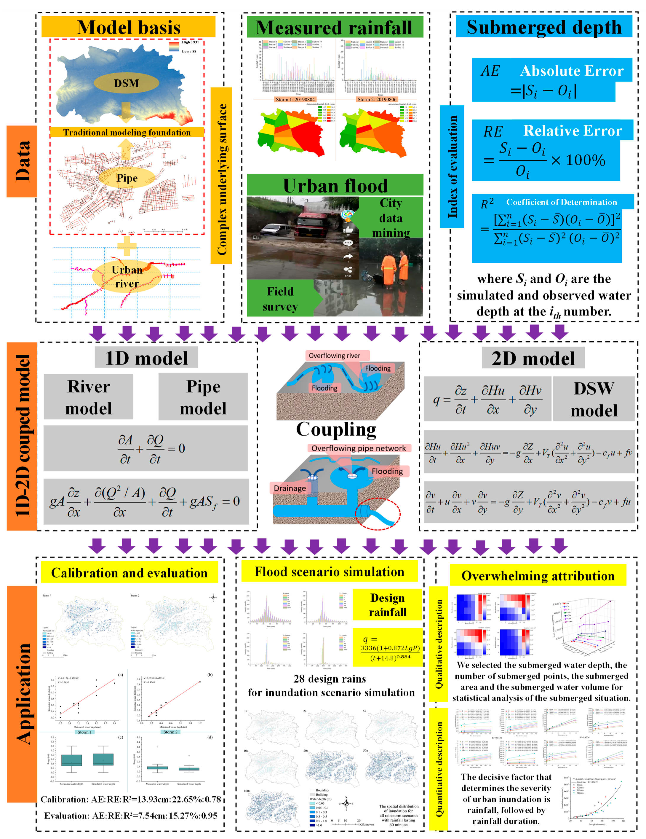
This paper first introduces a newly established model based on river model, surface model, and pipe model coupled underground drainage systems, river networks, and surface flows (As show in Figure 1). This 2D model is efficient for shallow-water flows and uses the lower–upper symmetric Gauss–Seidel (LU-SGS) implicit dual time-stepping method based on structured grids. Then, we explore the urban inundation response to rainstorm duration in a case study of the Luoyang City Center. Finally, based on the 1D–2D coupled model, taking into account multiple elements such as urban pipe network, topography, drainage canals, rivers, buildings, etc., we construct a storm and flood coupling model under the complex underlying surface conditions of the city, and realize the coupling of ground overflow–pipe network confluence–river confluence flood inundation simulation and the heavy rain scenario application.
2. Materials and Methods
2.1. Study Site
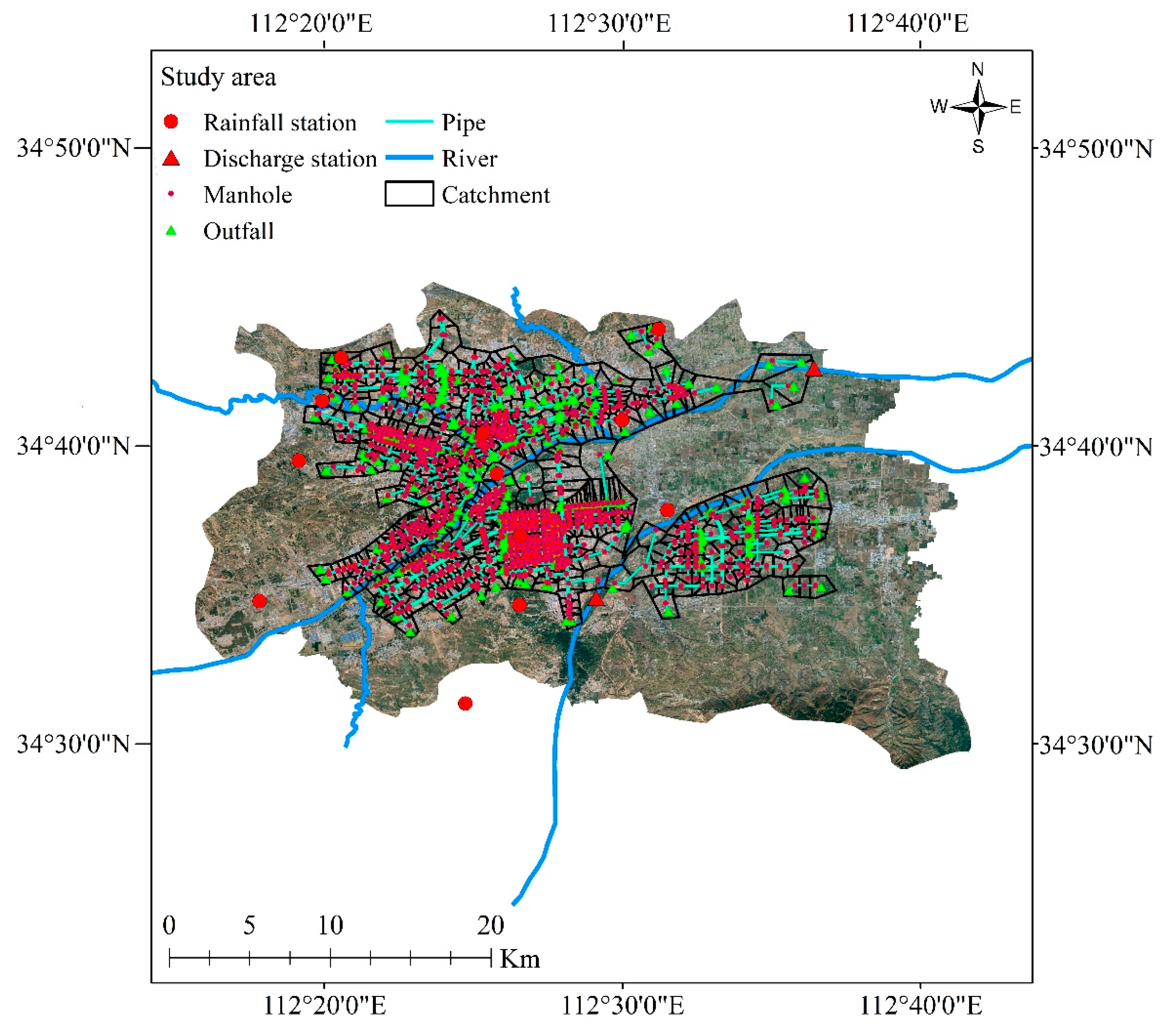
We selected Luoyang city center, in the northern Henan Province of China, as our study area (34°29′06″–34°45′47″ N, 112°15′44″–112°41′57″ E) (Figure 2). Luoyang city center, which constitutes the northern part of Luoyang city, is a typical small basin city with 803 km2 and is situated within the Yi-Luo River Basin. The two rivers of Yi he and Luo he passed through the downtown area of Luoyang.
The annual average temperature and rainfall are 14.6 °C and 600.2 mm, and the period of June to September accounted for 63.3% of the yearly precipitation. The study area has a semi-arid region with an average water surface evaporation of 1200 mm. Luoyang city center is a highly urbanized area, containing numerous businesses, campuses, and residential areas. The coverage of the impervious regions reaches 72%.
Although Luoyang city center is a newly developed area, its sewer system is insufficient for its current drainage needs. Most of the sewer system is designed for one- or two-year return periods. Thus, inundation is a regular occurrence during rainstorms in the Luoyang city center. In 2019, a rainstorm hit the entire Luoyang City, causing direct economic losses of $9.693 million. Luoyang City experienced significant damage from that rainstorm, and many streets were severely flooded. Therefore, it is a suitable site to study the characteristics of rainfall-induced inundations.
2.2. Data Availability and Processing
2.2.1. Topographic Data
In this study, digital elevation models (DEM) are drawn from the Geospatial Data Cloud (http://www.gscloud.cn/sources/accessdata/421?pid=302, accessed on 1 June 2021) grid size of 5 m × 5 m to be used in dynamic urban modeling. In 2D surface water simulation, the accuracy of the elevation data of the underlying surface is particularly important. However, the publicly available DEM data do not contain elevation information such as roads and buildings, so this part needs to be modified. The specific method consists of superimposing road and building data layers onto the DEM layer using GIS spatial analysis technology, in which the elevation of DEM covered by road is subtracted by 0.3 meters. DEM elevation of building cover has 10 m added.
2.2.2. Drainage System Data
The drainage system data, provided by the Luoyang Drainage Management Bureau, contained geographic and geometric information on the pipes, maintenance holes, rivers, and storage areas (e.g., holding ponds). Rainwater and wastewater in the study area are drained separately. The diameters of the pipes ranged from 0.5 to 2.00 m, and the depths of the maintenance holes ranged from 1.00 to 5.00 m. There are five rivers in the research region: the Yi, Luo, Chan, Jian, and Ganshui rivers (Table 1). These rivers were improved artificially a few years ago, and most of their cross sections are now rectangular. Thus, the rivers were set as rectangular open channels in the model. There are eight artificial lakes in the study area, set as storage nodes in the model. Consequently, 3610 pipes and available channels, 4792 maintenance holes, 161 outfalls, and eight storages were included in the model (Figure 2).
2.2.3. Rainstorm Data
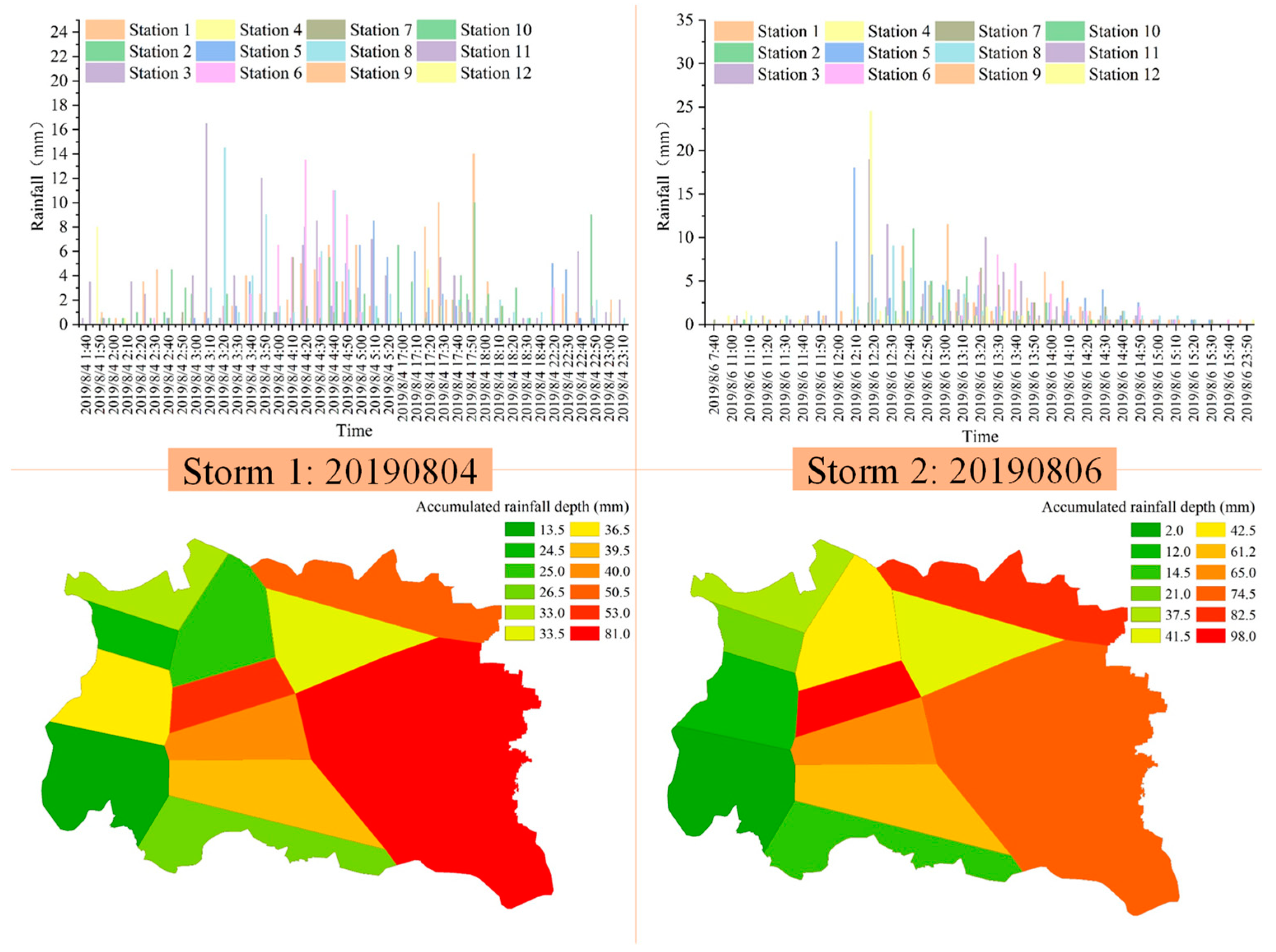
Two recorded historical rainstorms, Storm 1 and Storm 2 (Figure 3), were used to calibrate and evaluate the coupled model. These two rainstorms occurred on 4 August 2019, and 6 August 2019, respectively. The rainstorm data were obtained from the China Meteorological Data Service Center (http://cdc.nmic.cn/home.do, accessed on 1 June 2021).
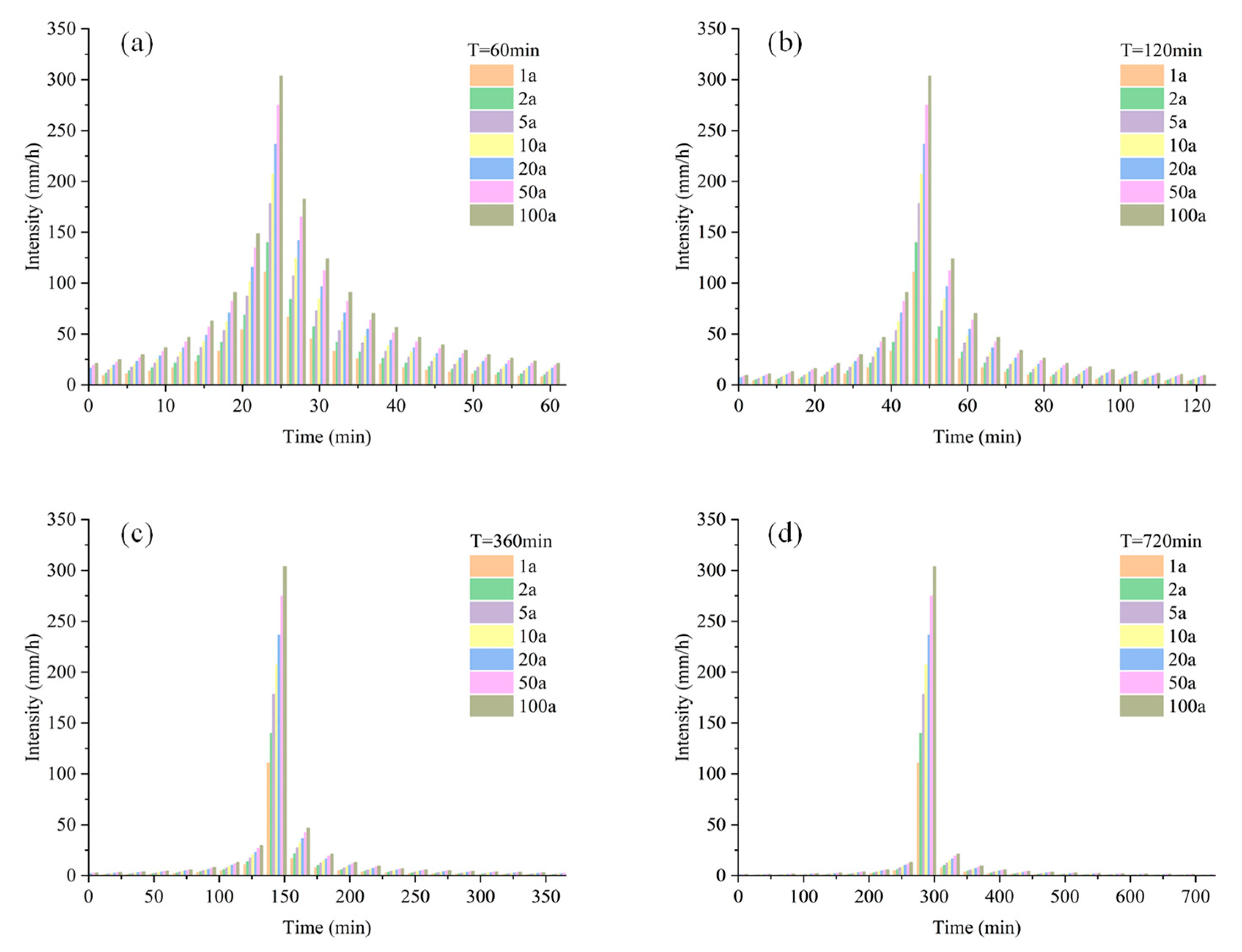
In addition, four patterns of rainstorms, with return periods of 1a, 2a, 5a, 10a, 20a, 50a, and 100a (Figure 4), were used as model inputs to study the inundation response. According to the Bureau of Municipal and Rural Construction, the rainfall intensity in Luoyang city can be summarized using Equation (1). The Chicago approach was used to redistribute the rainfall amounts before and after the peaks [23]. The main difference among the four rainstorm patterns was the position of the rainfall duration, and the rainfall durations were set to 60 min, 120 min, 360 min, and 720 min (Figure 4). We named these four rainstorms (Figure 4) Pattern 1, Pattern 2, Pattern 3, and Pattern 4.
where, is the rainfall intensity mm/hr; is the return period of rainstorms in yr; is the rainstorm duration in min.
2.3. 1D–2D Couples Model
We simultaneously simulated the flow dynamics in sewer networks, rivers, and overland surfaces by coupling the river, surface, and pipe models. The three models were executed individually at every time step and then connected through appropriate linkages to exchange the information obtained at suitable locations at the end of every step [24].
In general, flow exchange occurs at the connection between the surface flows and pipe or river flows. Thus, three types of linkages, including vertical, lateral, and longitudinal linkages, were implemented and studied. The relationships between these three models and the three linkages are presented in Figure 5.
2.3.1. Pipe and River Model
The confluence process of the pipeline and river channel can be approximated as flood wave movement without side flow. The 1D hydrodynamic method is based on the complete one-dimensional St. Vennat flow equation and has the best application effect, so it is used to simulate the flow movement of stormwater pipe network and river channel. [25,26].
The basic equations of the one-dimensional hydrodynamic model are as follows:
where Q is the discharge, A is the area of the cross section, H is water depth and Sf is friction gradient [27].
2.3.2. DSW Model
Combining the momentum equation in 2D form of the diffusion wave approximation with mass conservation yields, known as the diffusive wave approximation of the shallow water (DSW) equations, which was used to simulate the surface water inundation process in this study [25,28].
The basic principles of the two-dimensional hydrodynamic calculation model are as follows:
where u and v are the velocities in the Cartesian directions, g is the gravitational acceleration, VT is the horizontal eddy viscosity coefficient, cf is the bottom friction coefficient, and f is the Coriolis parameter [29].
2.4. Model Evaluation Indicator Selection
2.4.1. Absolute Error
The absolute error (AE) is the total value of the difference between the measured value and the actual value. Here, it refers to the total value of the difference between the simulated water depth of the model and the actual measured water depth. The mathematical expression is as follows:
where, Si and Oi are the simulated and observed water depth at the ith number [30].
2.4.2. Relative Error
Relative error (RE) refers to the value obtained by multiplying the ratio of the absolute error caused by the measurement to the measured (conventional) actual value by 100%, expressed as a percentage. Generally speaking, the relative error can better reflect the credibility of the measurement. It is mainly used to evaluate urban rain and flood models to indicate the credibility of the simulated value of flood peak discharge. It is described as follows:
where, Si and Oi are the simulated and observed water depth at the ith number [30].
2.4.3. The Coefficient of Determination
The coefficient of determination (R2) is often used to describe the degree of fit between data. When R2 is closer to 1, it means that the reference value of the related equation is higher; on the contrary, when it is closer to 0, it means that the reference value is lower. It is described as follows:
where, n is the total number of measured data, Si is the simulated water depth for data point, Oi is the measured water depth for data point , and is the averaged value of the measured water depth [30].
2.4.4. Nash–Sutcliffe Efficiency
The mathematical expressions of this metric can be described as follows:
where (m3/s) and (m3/s) represent the discharge of the observed and simulated hydrographs, respectively; is the mean value of the observed discharge, and n is the data points number. NSE measures the ability of the model to predict variables different from the mean, gives the proportion of the initial variance accounted for by the model, and ranges from 1 (perfect fit) to −∞. Values closer to 1 provide more accurate predictions [31].
3. Result and Discussion
3.1. Coupled Model Calibration and Evaluation
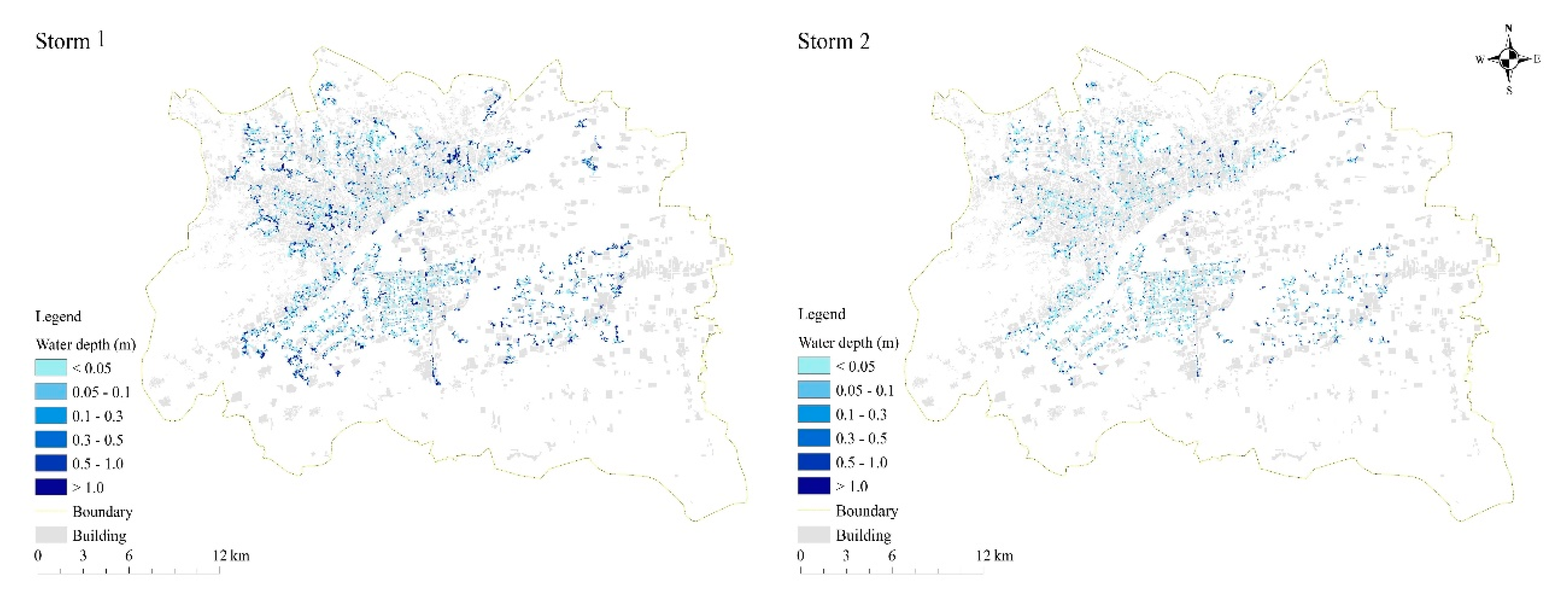
Two recorded historical rainstorms, storms 1 and 2, were used to calibrate and validate the coupled model (Figure 6). Due to data limitations, the calibration and validation criteria mainly focused on surface inundation depths and extent [32]. The traditional lumped hydrological model requires multiple flood process data to calibrate the model parameters in order to obtain the best model parameters on average [31]. However, the quality of modeling data itself is the main factor determining the accuracy of the 1D–2D hydrodynamic coupling model [33]. Therefore, the only parameters to be adjusted in this study are the Manning coefficient and model operation time step. The Manning coefficient is determined by experience, and the time step is 2 seconds. This is where the advantages of distributed physical hydrology lie, and the past application experience of the 1D–2D coupled model has also proved this point. [25].
The coupling model was calibrated and verified with the submerged water depths of 16 survey points in 2 historical storms and flood events (Table 2 and Table 3). The average relative error of the calibration-simulated water depth was 22.65%, and the average absolute error was 13.93 cm; the average relative error of the verified simulated water depth was 15.27%. The average absolute error is 7.54 cm.
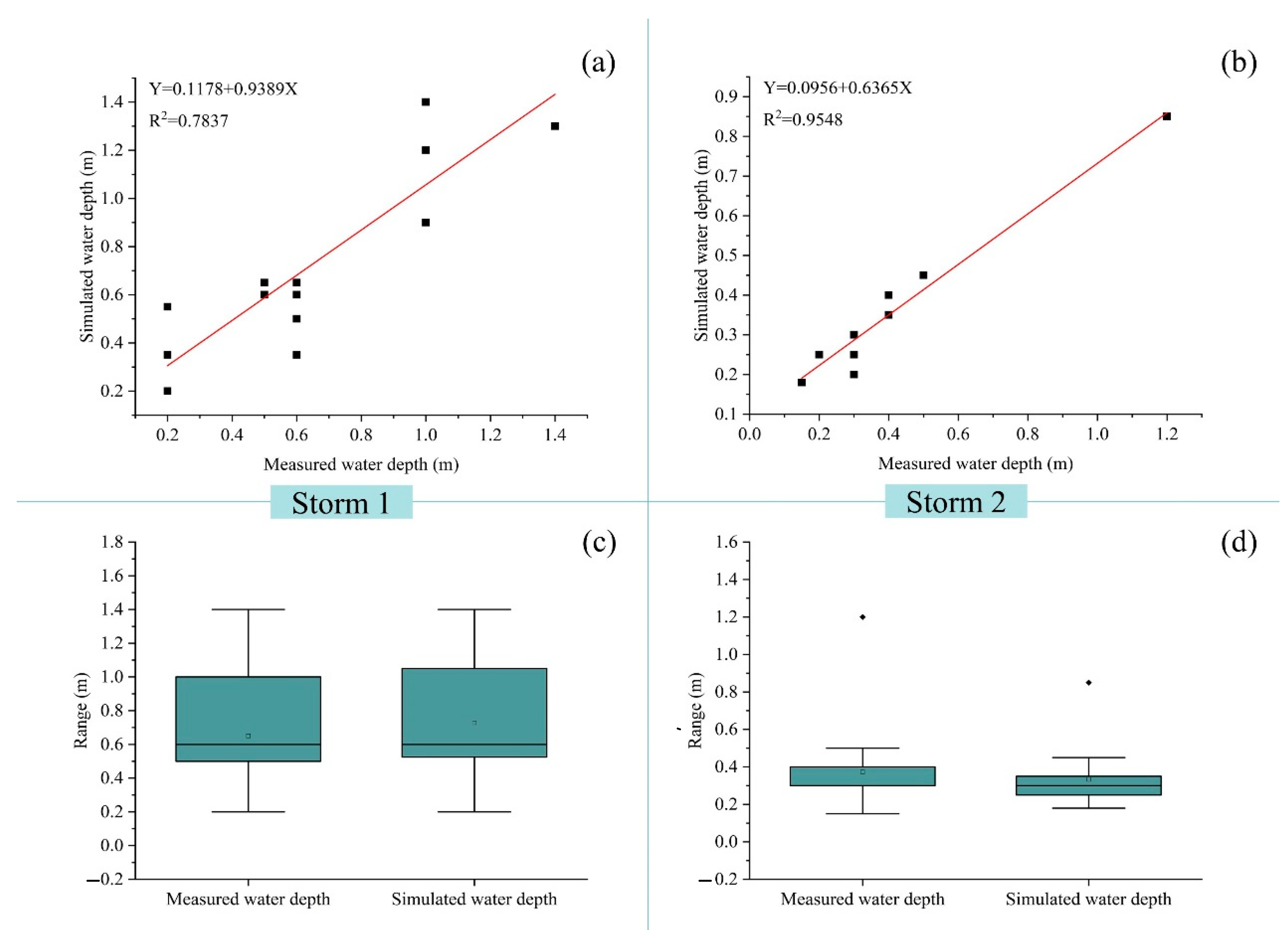
We conducted data analysis on the simulation results of two flood events (Figure 7). The R2 of the simulated and measured water depths of the 16 water accumulation points in the calibration period was 0.7837, and the R2 in the verification period was 0.9548. The overall simulation results during the calibration period are within a reasonable range. The measured water depth is 1.20 meters, the simulated water depth is 0.85 meters, and the AE is 0.35 meters. However, the RE is 29.2%, which is also within a reasonable range.
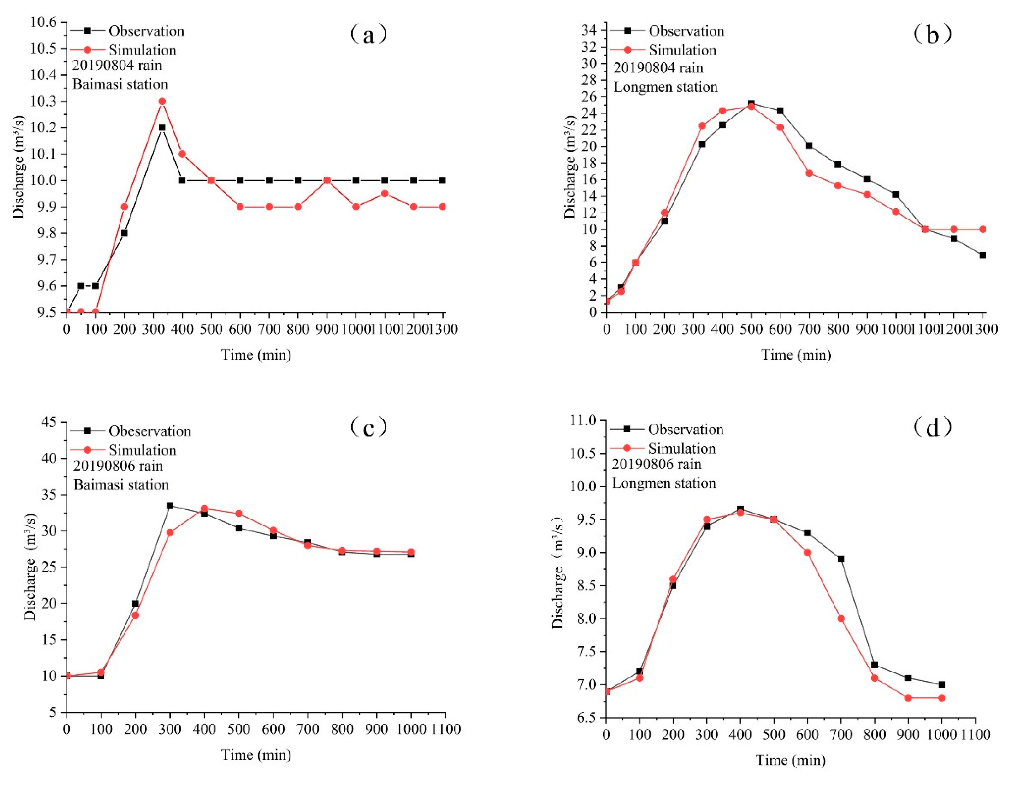
For the reliability of the results, this study verified the simulated flow of the river network model. The results are shown in Figure 8.
After simulation calculations, the NSE during the simulation calibration period for Baimasi Station and Longmen Station in 20190804 were 0.79 and 0.94, respectively; the NSE during the simulation verification period for Baimasi Station and Longmen Station in 20190806 were 0.96 and 0.91, respectively; therefore, the model simulation results are considered to be good.
3.2. Inundation Result under Four Different Rainstorm Patterns
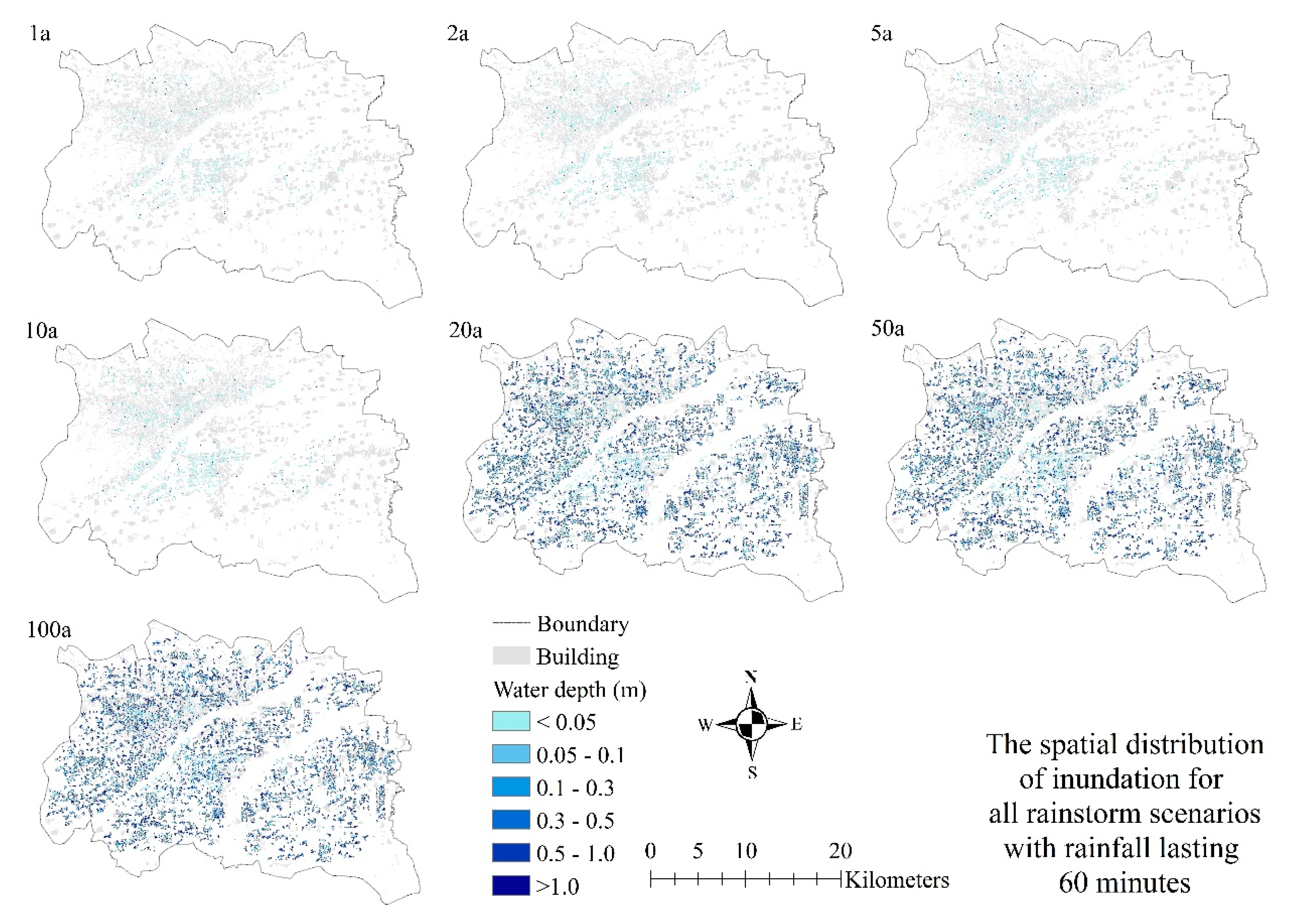
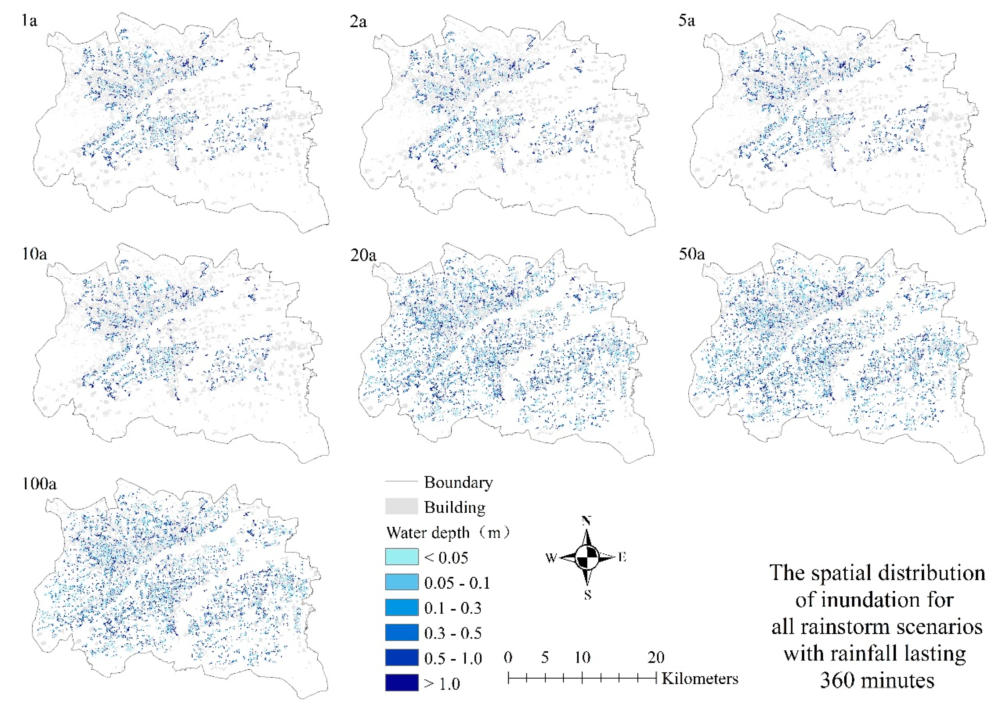
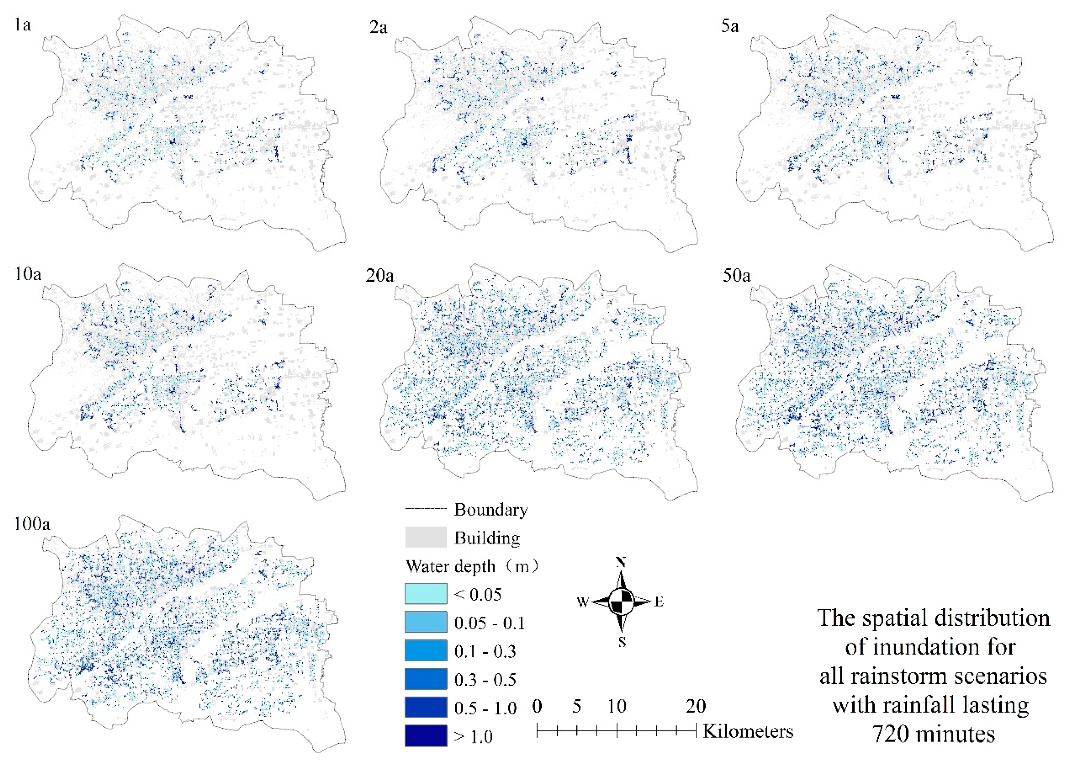
To explore the relationship between the amount of urban flood inundation on the amount of rainfall and rainfall duration, we designed the return periods of 1a, 2a, 5a, 10a, 20a, 50a, 100a with the rainfall duration of 60 min, 120 min, 360 min, 720 min. A total of 28 rainstorms were simulated and calculated by storm inundation (Figure 9, Figure 10, Figure 11 and Figure 12). The spatiotemporal results are presented in Section 3.2.1, Section 3.2.2 and Section 3.2.3. The flooded area of densely constructed central urban regions is more significant than that of suburban areas from flooding locations. The greater the amount of rainfall during the event, the greater the submerged area and water depth. This explains the frequent occurrence of flooding disasters when the city encounters rainfall. This poses a severe hazard to the safety of urban traffic, pedestrians, and vehicles. Therefore, effectively simulating the degree of inundation by heavy rains and floods in urban areas has important practical significance for urban flood control, disaster reduction and traffic emergency management, and is capable of providing necessary scientific and technological support for solving urban waterlogging problems [34].
3.2.1. Total Inundation Volumes
We know that the maximum amount of inundated water is an important indicator of measuring urban flood disasters. The maximum amount of inundated water here refers to the sum of the excess water volume after the pipeline overflows, the river overflows volume to the urban surface and the urban surface itself is full.
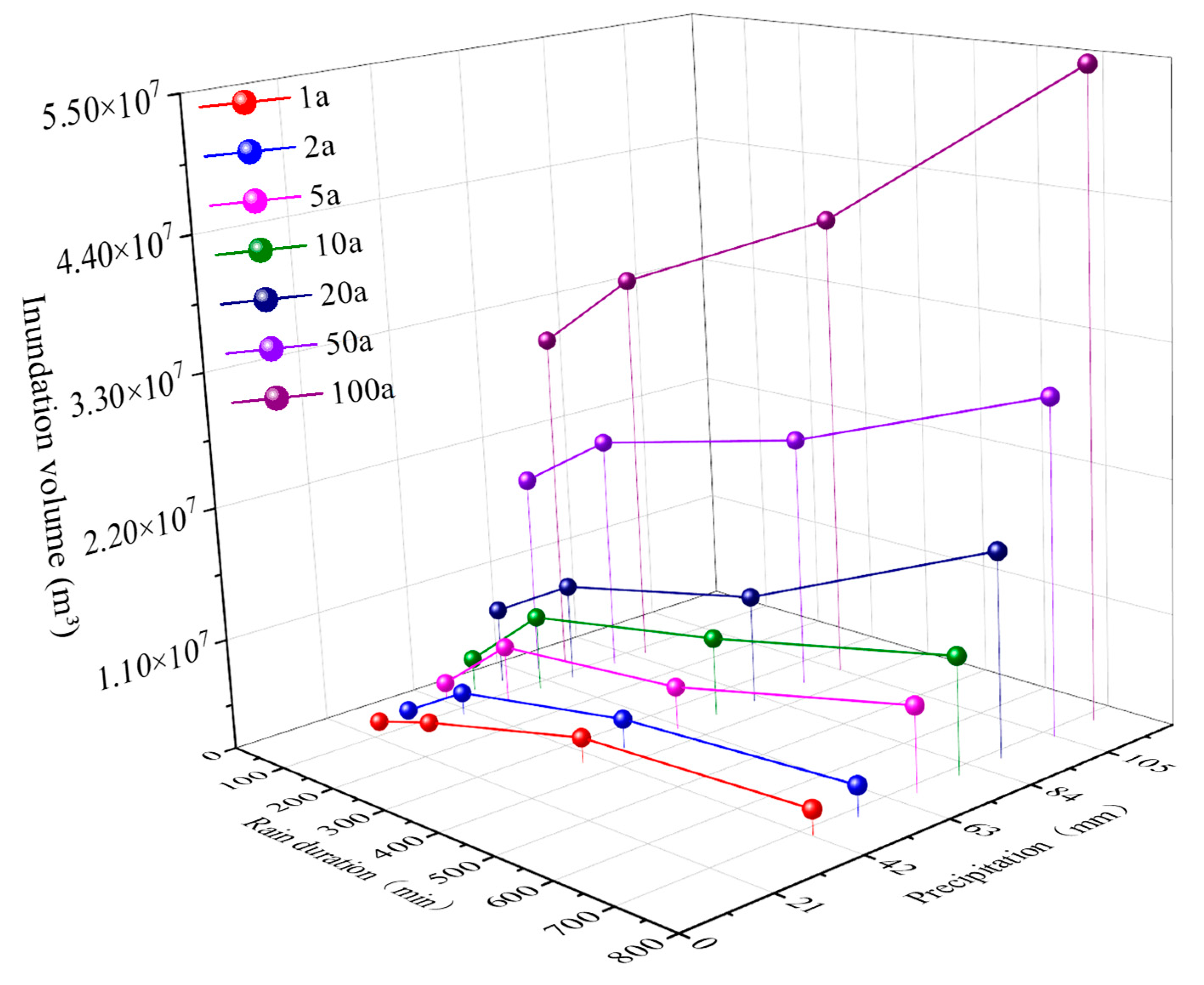
Table 4 presents the peak inundation volumes in each rainstorm, ranging from 1,804,911.66 m3 to 24,064,675.2 m3, 2,091,859.56 m3 to 31,751,228.07 m3, 3,943,031.4 m3 to 44,463,856.5 m3, and 3,875,545.08 m3 to 54,559,375.68 m3 for patterns 1, 2, 3, and 4. The 28 rainfall scenarios set will all be flooded, and the amount of flooded water shows a trend of increasing with the increase of rainfall duration and return period, respectively. Under the condition that the return period is 1 to 2 years, inundation will also occur; this shows that the urban drainage capacity is insufficient, which is also one of the direct causes of urban waterlogging (Figure 13).
3.2.2. Inundation Positions and Depths
Cities, especially central cities, have concentrated dense buildings and populations. Once urban flooding occurs, it will cause inevitable losses. Therefore, it is crucial to simulate the spatial distribution of urban inundation scenarios.
Figure 9, Figure 10, Figure 11 and Figure 12 shows the submerged space distribution under four rain patterns, highlighting the differences in the degree of inundation and spatial distribution. Even during the same return period, there were considerable differences in the inundation extent between different rain durations. The overall trend is that the submerged water depth and submerged area become more significant as rainfall increases. The inundation extents of Pattern 2 were close to those of Pattern 3, and the extents of Pattern 3 were comparable to those of Pattern 4. (Figure 13)
Table 5 presents the average submerged depth in each rainstorm, ranging from 0.1242 m to 1.0040 m, 0.1246 m to 1.2123 m, 0.1635 m to 1.2425 m, and 0.1564 m to1.4817 m for patterns 1, 2, 3, and 4. The results show that the longer the rainfall duration, the greater the average submerged depth. The greater the rainfall returns period, the greater the average submerged depth. This result is consistent with the amount of submerged water (Figure 13).
3.2.3. Inundation Area
After urban waterlogging, the submerged area is also one of the key indicators of measure severity. Table 6 presents the inundation area in each rainstorm, which ranged from 14.5323 km2 to 23.9688 km2, 16.7886 km2 to 26.1909 km2, 24.1164 km2 to 35.7858 km2, and 24.7797 km2 to 36.8217 km2 for patterns 1, 2, 3, and 4. Considering the spatial distribution (Figure 9, Figure 10, Figure 11 and Figure 12), the flooding situation is more serious in densely constructed areas, and the flooding area is relatively large.
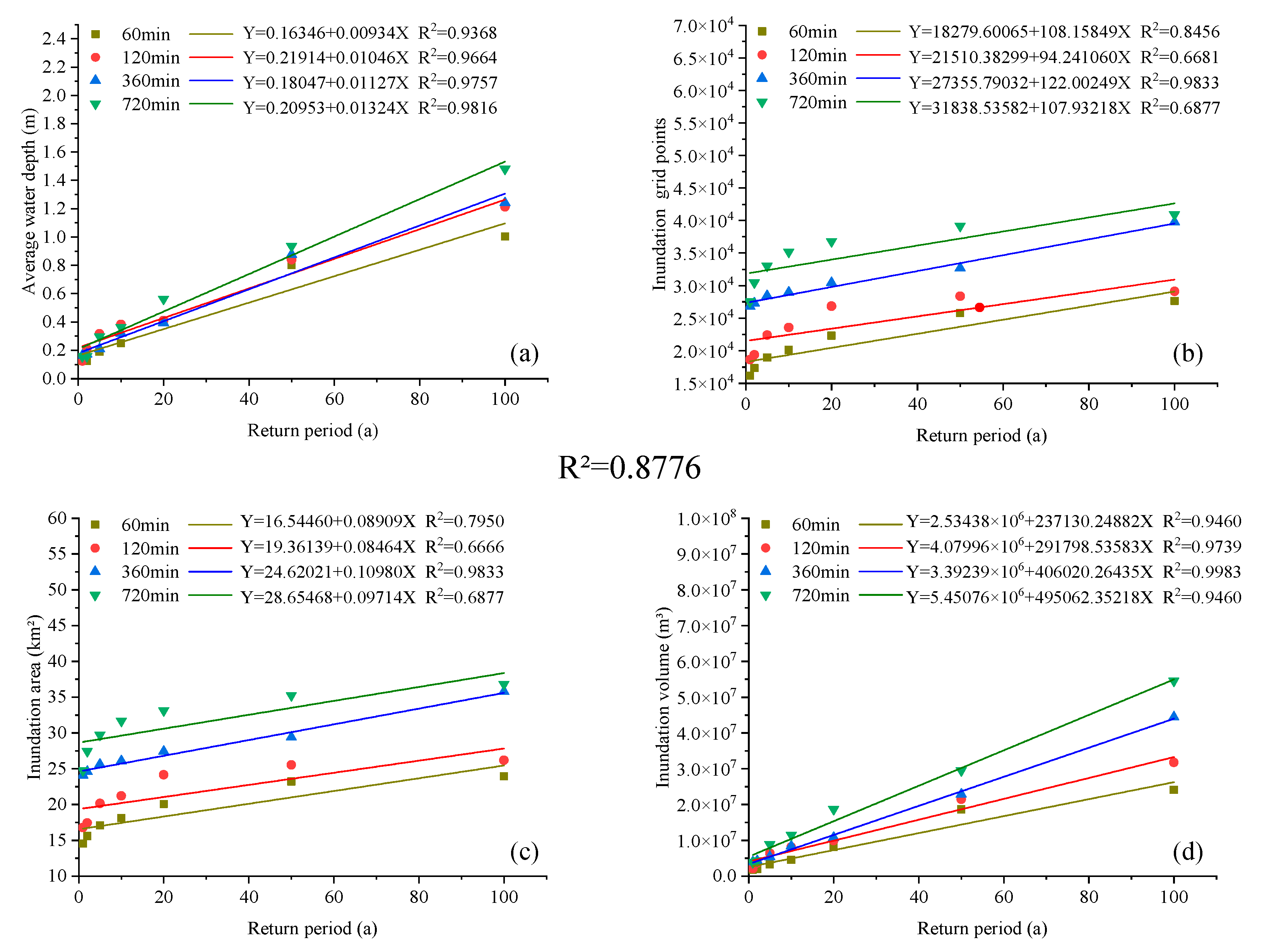
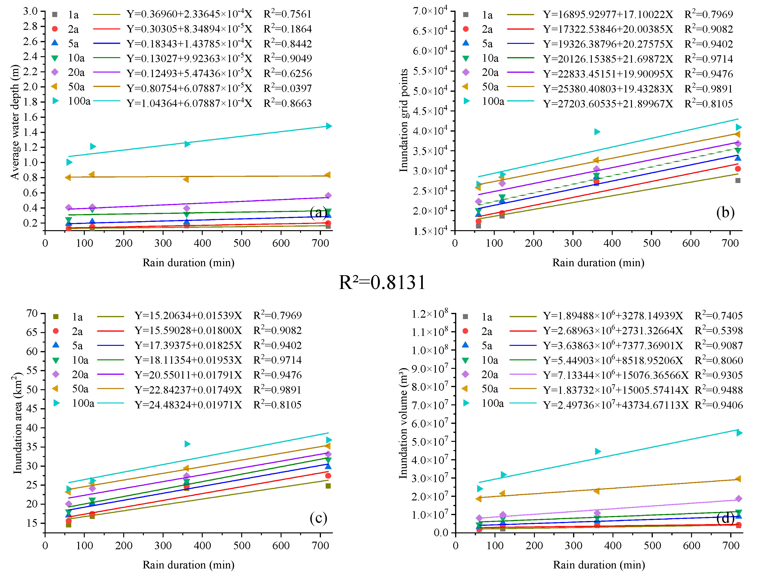
In this study, torrential rain and waterlogging simulation calculations were carried out in the downtown area of Luoyang. We selected the submerged water depth, the number of submerged points, the submerged area, and the submerged water volume for statistical analysis of the submerged situation (Figure 13). The study found that these four indicators are closely related to the rainfall return period and rainfall duration, and they all show a good linear relationship. The average correlation coefficient with the rainfall return period is 0.8776 (Figure 14), and the average correlation coefficient with the rainfall duration is 0.8131 (Figure 15). Therefore, it is concluded that the decisive factor determining the severity of urban inundation is rainfall, followed by rainfall duration.
4. Discussion
4.1. The Rationality of Coupling Model Construction
As we all know, a city is a region, not a closed watershed. Therefore, when considering inland river overflow and waterlogging, since the upstream and downstream of the river are considered to be the city’s boundaries, it is necessary to pay attention to whether the boundary condition is an input of the upper and lower rivers in line with reality [27,29]. In this study, the urban inland river system is considered: the upstream uses the measured flow as input, and the downstream uses the measured flow as output. Secondly, the model constructed by this research adopts the two-by-two connection method for the coupling of the drainage network, river, and surface, which is in line with the actual situation. The 1D–2D coupled model is a distributed hydrological model with full physical meaning. Therefore, the parameter calibration only needs to adjust the time step to ensure that the model calculation results do not diverge [22]. The measured water depth is compared with the simulated water depth to verify results and achieve better accuracy. Therefore, the coupling model constructed in this study is reasonable [33]. It is also worth studying the spatial boundary scale dependence of flood forecasting model, which is of great significance for urban flood risk assessment. This study is based on a coupled hydrological, hydrodynamic and physical mechanism model for flood risk assessment. The non-effective boundary is simply determined according to the administrative area, which also facilitates the planning of flood control work by the competent government departments. However, from the perspective of academic research, urban flood risk assessment should include interdisciplinary topics such as urban science, statistics, meteorology and computers [35]. Therefore, the diversification of research methods is also the future research direction.
All inland rivers in Luoyang have been artificially treated. The shape of the rivers is regular, and the bank slope protection is given mostly as a single building material. This also reduces the computational complexity of the model and indirectly improves the simulation accuracy.
4.2. Relationship between Inundation Volume and Rainfall Duration
It can be seen from the previous conclusion that the two rainfall elements that have a greater impact on flood inundation are rainfall and rainfall duration. Therefore, we analyze the correlation between the rainfall and the rainfall duration of the 28 design rains, the two main factors affecting inundation and the amount of inundation.
As shown in Figure 16, there is no doubt that the more significant the rainfall, the greater the flooding. However, Figure 16 also shows that the longer the rainfall duration, the greater the inundation. This is because as the rainfall duration in Chicago increases, the rainfall will concentrate in local periods, and the rainfall will become "thin", leading to increased water inundation. Refs. [23,32] In contrast. We also conducted detailed and rigorous discussion and research on this. In the study, we designed 28 rainfalls using the Chicago rain pattern and used it as the rainfall input of the coupling model. To avoid the complexity of the research results, we uniformly set the rain front coefficient to 0.4. That is to say, the proportion of the rain fronts of 28 rains is the same, which leads to a longer rainfall duration, more prominent the rain peaks, and a more concentrated majority of the rainfall of a rain. This leads to a trend that the longer the rainfall lasts, the greater the amount of flooding. In fact, this is not inconsistent with the common-sense conclusion mentioned earlier, and even indirectly confirms this conclusion.
4.3. Relationship between Inundation Volume and Precipitation
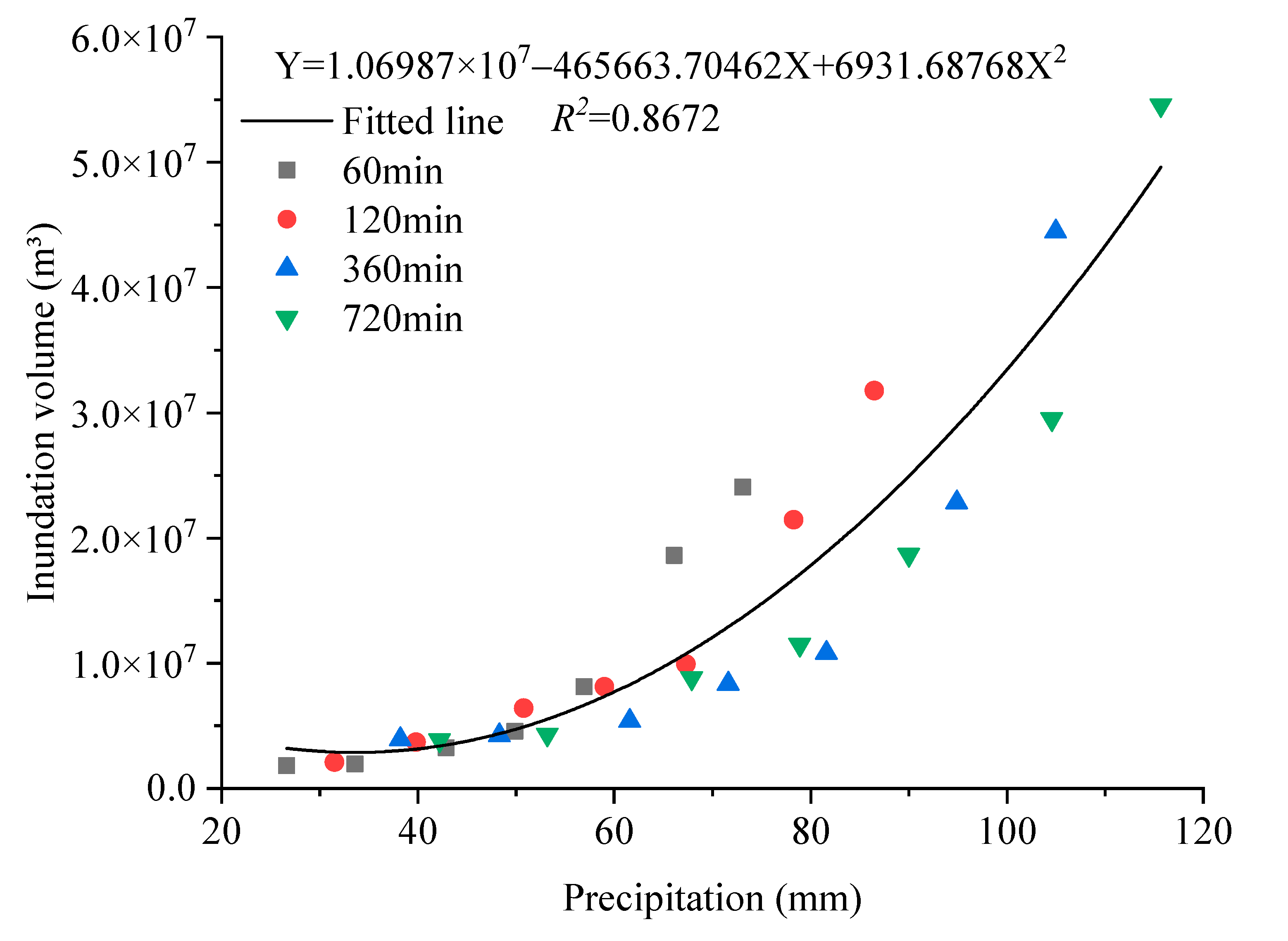
Based on the research results, we have compared and analyzed the correlation between rainfall and inundation (Figure 17), giving a quantitative description it. Rainfall and inundation show a good secondary correlation; R2 is 0.8672, which is helpful to the study of the relationship between urban waterlogging and rainfall threshold.
The uncertainty of rainfall input is the largest source of simulation errors in the urban rain flood model. Rainfall alone includes rainfall, rainfall duration, rain peak location, input events, rainfall sources, and other internal factors. This study only discusses rainfall and rainfall duration as its two main factors. The influence of different factors on the urban rainwater model needs further investigation. Multi-source rainfall input is a research approach. In the current information explosion era, big data technology uses big data to effectively crawl network data as the rainfall model input; this is a topic of intense interest in current urban hydrological research. How to transform unstructured data into structured data and use dense data to drive urban rain and flood models will be the focus of future research [35].
5. Conclusions
This research puts forward the construction method of urban rain and flood model based on the complex underlying surface of the city and explains the principle of urban waterlogging. Based on the one-dimensional–two-dimensional hydrodynamic method, the urban flood coupling model of surface overflow–pipe network overflow–river course overflow was successfully constructed and applied in examples. According to rainfall–inundation, we have systematically discussed the correlation between rainfall and rainfall duration on urban inundation. The main conclusions are as follows:
Based on the 1D–2D couple models, a coupled urban storm and flood model considering one-dimensional river channels, two-dimensional ground, and underground pipe networks are constructed. Among them, the river model is used to calculate the flood evolution and overflow inundation process of urban inland rivers; the pipe model is used to build a simulated urban underground pipeline network flow calculation and rainwater well overflow inundation process; the surface model is used to simulate two-dimensional surface overflow of pipe networks and rivers calculation. The above three models were coupled in together. The construction of a one-dimensional and two-dimensional coupled urban flood model and flood simulation was realized with the Luoyang city center as a pilot.
We selected the submerged water depths of 16 survey points in two historical storms and flood events to calibrate and verify the coupled model. The average relative error of simulated water depth during the calibration period was 22.65%, the average absolute error was 13.93 cm, and R2 was 0.7835; the average relative error of the simulated water depth during the verification period was 15.27%, the average absolute error was 7.54 cm, and R2 was 0.9548. The simulation results are promising.
We designed 28 rains with a return period of 1a, 2a, 5a, 10a, 20a, 50a, 100a, and rainfall duration of 60 min, 120 min, 360 min, and 720 min, to simulate and analyze the rainstorm inundation in the downtown area of Luoyang. The calculation results were as follows: under the same return period, the shorter was the rainfall duration, the faster the formation of inundation, the longer the rainfall duration, the longer the inundation duration; the greater was the return period, the longer the rainfall duration, and the greater the maximum flooding water volume. Corresponding submerged time, submerged water depth, and maximum submerged water volume in dense building areas were calculated. The R2 of rainfall and urban rainstorm inundation was 0.8776, and the R2 of rainfall duration and urban rainstorm inundation was 0.8141. Therefore, the influencing factor that determines the magnitude of inundation is rainfall, followed by rainfall duration.
Author Contributions
For this research paper with several authors, a short paragraph specifying their individual contributions was provided. G.L. and C.L. developed the original idea and contributed to the research design for the study. H.Z. was responsible for data collecting. J.W. provided guidance and improving suggestion. F.Y. provided some guidance for the writing of the article. All authors have read and agreed to the published version of the manuscript.
Funding
This work was funded by Key projects of National Natural Science Foundation of China (51739009), Department of Water Resources of Henan Province (GG202068), National Natural Science Foundation of China (51979250).
Data Availability Statement
Not applicable. The data in this manuscript is also used in other ongoing research, so data and materials are not applicable.
Conflicts of Interest
The authors declare that there is no conflict of interest regarding the publication of this paper.
References
- Grimm, N.B.; Faeth, S.H.; Golubiewski, N.E.; Redman, C.L.; Wu, J.; Bai, X.; Briggs, J.M. Global change and the ecology of cities. Science 2008, 319, 756–760. [Google Scholar] [CrossRef] [PubMed] [Green Version]
- Wang, J.Y.; Hu, C.H.; Ma, B.Y.; Mu, X.L. Rapid Urbanization Impact on the Hydrological Processes in Zhengzhou, China. Water 2020, 12, 1870. [Google Scholar] [CrossRef]
- Dong, X.; Huang, S.; Zeng, S. Design and evaluation of control strategies in urban drainage systems in Kunming city. Front. Environ. Sci. Eng. 2017, 11, 13. [Google Scholar] [CrossRef]
- Xing, Y.; Liang, Q.H.; Wang, G.; Ming, X.D.; Xia, X.L. City-scale hydrodynamic modelling of urban flash floods: The issues of scale and resolution. Nat. Hazards 2019, 96, 473–496. [Google Scholar] [CrossRef] [Green Version]
- Turner, A.; Sahin, O.; Giurco, D.; Stewart, R.; Porter, M. The potential role of desalination in managing flood risks from dam overflows: The case of Sydney, Australia. J. Clean. Prod. 2016, 135, 342–355. [Google Scholar] [CrossRef] [Green Version]
- Pasquier, U.; He, Y.; Hooton, S.; Goulden, M.; Hiscock, K.M. An integrated 1D-2D hydraulic modelling approach to assess the sensitivity of a coastal region to compound flooding hazard under climate change. Nat. Hazards 2019, 98, 915–937. [Google Scholar] [CrossRef] [Green Version]
- Lyu, H.M.; Shen, S.L.; Zhou, A.N.; Yang, J. Perspectives for flood risk assessment and management for mega-city metro system. Tunn. Undergr. Space Technol. 2019, 84, 31–44. [Google Scholar] [CrossRef]
- Gao, Y.; Yuan, Y.; Wang, H.; Zhang, Z.; Ye, L. Analysis of impacts of polders on flood processes in Qinhuai River Basin, China, using the HEC-RAS model. Water Sci. Technol. Water Supply 2018, 18, 1852–1860. [Google Scholar] [CrossRef] [Green Version]
- Jiao, S.; Zhang, X.; Xu, Y. A review of Chinese land suitability assessment from the rainfall-waterlogging perspective: Evidence from the Su Yu Yuan area. J. Clean. Prod. 2017, 144, 100–106. [Google Scholar] [CrossRef]
- Mehta, D.J.; Ramani, M.M.; Joshi, M.M. Application of 1-D HEC-RAS model in design of channels. Methodology 2013, 1, 4–62. [Google Scholar]
- Bach, P.M.; Rauch, W.; Mikkelsen, P.S.; McCarthy, D.T.; Deletic, A. A critical review of integrated urban water modelling Urban drainage and beyond. Environ. Model. Softw. 2014, 54, 88–107. [Google Scholar] [CrossRef]
- Mei, C. Urban Hydrology and Hydrodynamic Coupling Model and Its Application Research. Ph.D. Thesis, China Institute of Water Resources and Hydropower Research, Beijing, China, 2019. [Google Scholar]
- Huang, G.-R.; Wang, X.; Huang, W. Simulation of Rainstorm Water Logging in Urban Area Based on InfoWorks ICM Model. Water Resour. Power 2017, 35, 66–70. [Google Scholar]
- Van Der Knijff, J.M.; Younis, J.; De Roo, A.P.J. LISFLOOD: 2010 a GIS-based distributed model for river basin scale water balance and flood simulation. Int. J. Geogr. Inf. Sci. 2010, 24, 189–212. [Google Scholar] [CrossRef]
- Liu, J.; Xia, L.; Mei, C.; Shao, W.; Yu, H.; Ma, J. Analysis of the role of deep tunnel drainage system in urban waterlogging prevention. J. Appl. Basic Sci. Eng. 2019, 27, 252–263. [Google Scholar]
- Lyu, H.M.; Shen, S.L.; Yang, J.; Yin, Z.Y. Inundation analysis of metro systems with the storm water management model incorporated into a geographical information system: A case study in Shanghai. Hydrol. Earth Syst. Sci. 2019, 23, 4293–4307. [Google Scholar] [CrossRef] [Green Version]
- Zischg, A.P.; Mosimann, M.; Bernet, D.B.; Rothlisberger, V. Validation of 2D flood models with insurance claims. J. Hydrol. 2018, 557, 350–361. [Google Scholar] [CrossRef] [Green Version]
- Martins, R.; Leandro, J.; Djordjevic, S. Influence of sewer network models on urban flood damage assessment based on coupled 1D/2D models. J. Flood Risk Manag. 2018, 11, S717–S728. [Google Scholar] [CrossRef]
- Fraga, I.; Cea, L.; Puertas, J. Validation of a 1D-2D dual drainage model under unsteady part-full and surcharged sewer conditions. Urban Water J. 2017, 14, 74–84. [Google Scholar] [CrossRef]
- Leandro, J.; Schumann, A.; Pfister, A. A step towards considering the spatial heterogeneity of urban key features in urban hydrology flood modelling. J. Hydrol. 2016, 535, 356–365. [Google Scholar] [CrossRef]
- van der Sterren, M.; Rahman, A.; Ryan, G. Modeling of a lot scale rainwater tank system in XP-SWMM: A case study in Western Sydney, Australia. J. Environ. Manag. 2014, 141, 177–189. [Google Scholar] [CrossRef]
- Gong, Y.; Li, X.; Zhai, D.; Yin, D.; Song, R.; Li, J.; Yuan, D. Influence of Rainfall, Model Parameters and Routing Methods on Stormwater Modelling. Water Resour. Manag. 2018, 32, 735–750. [Google Scholar] [CrossRef]
- Cheng, M.; Qin, H.; Fu, G.; He, K. Performance evaluation of time-sharing utilization of multi-function sponge space to reduce waterlogging in a highly urbanizing area. J. Environ. Manag. 2020, 269, 110760. [Google Scholar] [CrossRef] [PubMed]
- Bruni, G.; Reinoso, R.; van de Giesen, N.C.; Clemens, F.H.L.R.; ten Veldhuis, J.A.E. On the sensitivity of urban hydrodynamic modelling to rainfall spatial and temporal resolution. Hydrol. Earth Syst. Sci. 2015, 19, 691–709. [Google Scholar] [CrossRef]
- Bermudez, M.; Ntegeka, V.; Wolfs, V.; Willens, P. Development and Comparison of Two Fast Surrogate Models for Urban Pluvial Flood Simulations. Water Resour. Manag. 2018, 32, 2801–2815. [Google Scholar] [CrossRef]
- Yu, D.; Yin, J.; Liu, M. Validating city-scale surface water flood modelling using crowd-sourced data. Environ. Res. Lett. 2016, 11, 124011. [Google Scholar] [CrossRef]
- Chen, W.J.; Huang, G.R.; Zhang, H.; Wang, W.Q. Urban inundation response to rainstorm patterns with a coupled hydrodynamic model: A case study in Haidian Island, China. J. Hydrol. 2018, 564, 1022–1035. [Google Scholar] [CrossRef]
- Jang, J.-H. An Advanced Method to Apply Multiple Rainfall Thresholds for Urban Flood Warnings. Water 2015, 7, 6056–6078. [Google Scholar] [CrossRef] [Green Version]
- Hu, C.H.; Liu, C.S.; Yao, Y.C.; Wu, Q.; Ma, B.Y.; Jian, S.Q. Evaluation of the Impact of Rainfall Inputs on Urban Rainfall Models: A Systematic Review. Water 2020, 12, 2484. [Google Scholar] [CrossRef]
- Nash, J.E.; Sutcliffe, J.V. River flow forecasting through conceptual models part I—A discussion of principles. J. Hydrol. 1970, 10, 282–290. [Google Scholar] [CrossRef]
- Indrawati, D.; Yakti, B.; Purwanti, A.; Hadinagoro, R. Computing urban flooding of meandering river using 2D numerical model (case study: Kebon Jati-Kalibata segment, Ciliwung river basin). In Proceedings of the 2nd Conference for Civil Engineering Research Networks; Inst Teknologi Bandung, Fac Civil & Environm Engn: Bandung, Indonesia, 2019; Volume 270. [Google Scholar]
- Kim, S.E.; Lee, S.; Kim, D.; Song, C.G. Stormwater Inundation Analysis in Small and Medium Cities for the Climate Change Using EPA-SWMM and HDM-2D. J. Coast. Res. 2018, 991–995. [Google Scholar] [CrossRef]
- Djordjevic, S.; Prodanovic, D.; Maksimovic, C.; Ivetic, M.; Savic, D. SIPSON—Simulation of interaction between pipe flow and surface overland flow in networks. Water Sci. Technol. 2005, 52, 275–283. [Google Scholar] [CrossRef] [PubMed]
- Zheng, Q.; Shen, S.L.; Zhou, A.; Lyu, H.M. Inundation risk assessment based on G-DEMATEL-AHP and its application to Zhengzhou flooding disaster. Sustain. Cities Soc. 2022, 86, 104138. [Google Scholar] [CrossRef]
- Lowe, R.; Urich, C.; Domingo, N.S.; Mark, O.; Deletic, A.; Arnbjerg-Nielsen, K. Assessment of urban pluvial flood risk and efficiency of adaptation options through simulations—A new generation of urban planning tools. J. Hydrol. 2017, 550, 355–367. [Google Scholar] [CrossRef]
Figure 1.
Schematic diagram of urban rain flood inundation principle. (Compared with natural watersheds, the underlying surface conditions of cities are more complicated. Urban floods also include three parts: pipe network overflow, river overflow, and surface overflow).
Figure 1.
Schematic diagram of urban rain flood inundation principle. (Compared with natural watersheds, the underlying surface conditions of cities are more complicated. Urban floods also include three parts: pipe network overflow, river overflow, and surface overflow).

Figure 2.
Research region and sewer system distribution. We selected Luoyang city center, in the northern Henan Province of China, as our study area (34°29′06″–34°45′47″ N, 112°15′44″–112°41′57″ E, at 150 m asl) (Figure 1). Luoyang city center, which constitutes the northern part of Luoyang city, is a typical small basin city with an area of 803 km2 and is situated within the Yi-Luo River Basin. The two rivers of Yi he and Luo he passed through the downtown area of Luoyang.

Figure 3.
Hydrographs of the two historical rainstorms (4 August 2019 and 6 August 2019). Storm 1 started at 1:40 and ended at 23:10 on 4 August 2019. It was a unimodal rainstorm, the first rainfall peak occurring at 3:10 with an intensity of 16.5 mm/h and the second rainfall peak occurring at 17:30 with an intensity of 5.5 mm/h. Storm 2 started at 7:40 and ended at 23:50, lasting about 22 h on 6 August 2019, with a maximum intensity of 24.0 mm/h occurring at 12:20. Figure 3 shows the hydrographs of the storms.

Figure 4.
Synthetic hyetograph of four rainstorm patterns. The main difference among the four rainstorm patterns is the position of the rainfall duration; The rainfall duration is set as 60 min, 120 minutes, 360 min and 720 min, which are respectively named as Pattern 1 (a), Pattern 2 (b), Pattern 3 (c) and Pattern 4 (d).

Figure 5.
1D–2D rainfall flood model coupling scheme (The process frame diagram of this study).

Figure 6.
Spatial distributions of inundations from Storm 1 and Storm 2.

Figure 7.
Comparison of simulated water depth and measured water depth of Storm 1 (a,c) and Storm 2 (b,d).
Figure 7.
Comparison of simulated water depth and measured water depth of Storm 1 (a,c) and Storm 2 (b,d).

Figure 8.
Comparison of simulated discharge and observed discharge of Storm 1 and Storm 2: (a) Discharge calibration of 20190804 rain in Baimasi station; (b) Discharge calibration of 20190804 rain in Longmen station; (c) Discharge evaluation of 20190806 rain in Baimasi station; (d) Discharge evaluation of 20190806 rain in Longmen station.

Figure 9.
Spatial distributions of inundation for 60 min rainstorm scenarios.

Figure 10.
Spatial distributions of inundation for 120 min rainstorm scenarios.

Figure 11.
Spatial distributions of inundation for 360 min rainstorm scenarios.

Figure 12.
Spatial distributions of inundation for 720 min rainstorm scenarios.

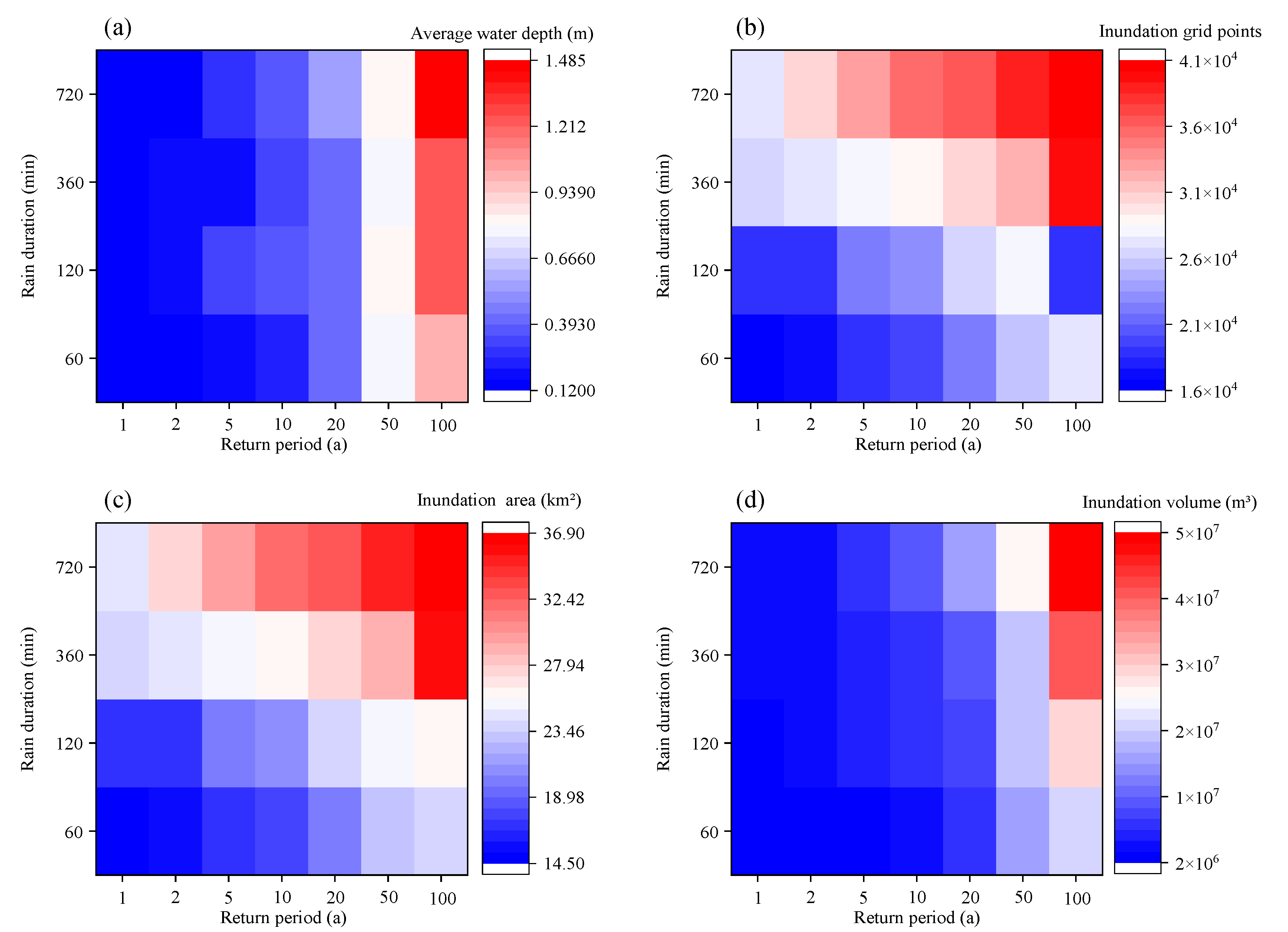
Figure 13.
(a) The relationship between the average submerged water depth, the return period and duration of rainfall. (b) The relationship between the number of submerged grid points and the rainfall return period and rainfall duration. (c) The relationship between submerged area and rainfall return period and rainfall duration. (d) The relationship between submerged water volume and rainfall return period and rainfall duration.

Figure 14.
Trend chart of relationship between submerged water depth (a), submerged grid points (b), submerged area (c), submerged water volume (d) and return period. (The return period and the four submergence indicators are linearly correlated, with an average R2 of 0.8776).
Figure 14.
Trend chart of relationship between submerged water depth (a), submerged grid points (b), submerged area (c), submerged water volume (d) and return period. (The return period and the four submergence indicators are linearly correlated, with an average R2 of 0.8776).

Figure 15.
Trend chart of relationship between submerged water depth(a), submerged grid points (b), submerged area (c), submerged water volume (d) and rain duration. (The rain duration and the four submergence indicators are linearly correlated, with an average R2 of 0.8131).
Figure 15.
Trend chart of relationship between submerged water depth(a), submerged grid points (b), submerged area (c), submerged water volume (d) and rain duration. (The rain duration and the four submergence indicators are linearly correlated, with an average R2 of 0.8131).

Figure 16.
The relationship between submerged water volume and rainfall duration and rainfall.

Figure 17.
The relationship between submerged water volume and Precipitation.


Table 1.
Basic information of Yi, Luo, Chan, Jian and Ganshui rivers.
| River Name | Channel Length (km) | Number of River Sections | Average Distance of Section (m) |
|---|---|---|---|
| Yi river | 23.2 | 32 | 725.0 |
| Luo river | 44.5 | 84 | 529.7 |
| Chan river | 10.4 | 31 | 322.6 |
| Jian river | 19.2 | 32 | 600.0 |
| Ganshui river | 7.6 | 16 | 475.0 |
Table 2.
Table of simulation results of flooding depth of water accumulation point in storm 1.
| Site Number | Road Section Name | Simulated Water Depth (m) | Measured Water Depth (m) | Absolute Error (m) | Relative Error (%) |
|---|---|---|---|---|---|
| 1 | Anju Road Railway Bridge Culvert | 0.60 | 0.50 | 0.10 | 20.0 |
| 2 | Luobai Road Anju Road Railway Bridge Culvert | 0.60 | 0.50 | 0.10 | 20.0 |
| 3 | Low-lying area of Taxi Village, Hanhe Hui District | 0.65 | 0.60 | 0.05 | 8.3 |
| 4 | Taikang Road Wangcheng Avenue Intersection to Xinyue Intersection | 0.65 | 0.50 | 0.05 | 10.0 |
| 5 | Niepan Road Jiaozhi Railway Bridge Culvert | 0.35 | 0.60 | 0.25 | 41.7 |
| 6 | Changchun Road, Jianxi District | 0.50 | 0.60 | 0.10 | 16.7 |
| 7 | Wanda Intersection | 0.60 | 0.60 | 0.05 | 8.3 |
| 8 | Sui-Tangcheng Road Longhai Railway Line Culvert | 0.20 | 0.20 | 0.01 | 5.0 |
| 9 | Guanlin Station Bridge, Erguang Expressway, Yibin District | 0.55 | 0.20 | 0.35 | 175.0 |
| 10 | Pingdeng Street Overpass, Chanhe District | 0.35 | 0.20 | 0.15 | 75.0 |
| 11 | Houzaimen Street, Yiren Road | 1.20 | 1.00 | 0.20 | 20.0 |
| 12 | Qiming East Road Jiaoliu Railway Bridge Culvert | 1.40 | 1.00 | 0.40 | 40.0 |
| 13 | Yiren Road, New District | 1.20 | 1.00 | 0.20 | 20.0 |
| 14 | East Huatan Overpass, Yanhe District | 0.90 | 1.00 | 0.10 | 10.0 |
| 15 | Longmen Avenue, Longmen North Bridge | 1.30 | 1.40 | 0.10 | 7.1 |
| 16 | Evergrande Oasis Section of East Zhongzhou Road | 0.60 | 0.50 | 0.10 | 20.0 |
Table 3.
Table of simulation results of flooding depth of water accumulation point in storm 2.
| Site Number | Road Section Name | Simulated Water Depth (m) | Measured Water Depth (m) | Absolute Error (m) | Relative Error (%) |
|---|---|---|---|---|---|
| 1 | Anju Road Railway Bridge Culvert | 0.30 | 0.30 | 0.05 | 16.7 |
| 2 | Luobai Road Anju Road Railway Bridge Culvert | 0.30 | 0.30 | 0.05 | 16.7 |
| 3 | Low-lying area of Taxi Village, Chanhe District | 0.40 | 0.40 | 0.05 | 12.5 |
| 4 | Taikang Road Wangcheng Avenue Intersection to Xinyue Intersection | 0.25 | 0.30 | 0.05 | 16.7 |
| 5 | Niepan Road Jiaozhi Railway Bridge Culvert | 0.25 | 0.20 | 0.05 | 0.25 |
| 6 | Changchun Road, Jianxi District | 0.25 | 0.20 | 0.05 | 0.25 |
| 7 | Wanda Intersection | 0.35 | 0.40 | 0.05 | 12.5 |
| 8 | Sui-Tangcheng Road Longhai Railway Line Culvert | 0.25 | 0.30 | 0.05 | 16.7 |
| 9 | Guanlin Station Bridge, Erguang Expressway, Yibin District | 0.85 | 1.20 | 0.35 | 29.2 |
| 10 | Pingping Street Overpass, Yanhe District | 0.30 | 0.30 | 0.05 | 16.7 |
| 11 | Houzaimen Street, Yiren Road | 0.18 | 0.15 | 0.03 | 20.0 |
| 12 | Qiming East Road Jiaoliu Railway Bridge Culvert | 0.45 | 0.50 | 0.05 | 10.0 |
| 13 | Yiren Road, New District | 0.20 | 0.30 | 0.10 | 33.3 |
| 14 | East Huatan Overpass, Yanhe District | 0.90 | 1.00 | 0.10 | 10.0 |
| 15 | Longmen Avenue, Longmen North Bridge | 1.30 | 1.40 | 0.10 | 7.1 |
| 16 | Evergrande Oasis Section of East Zhongzhou Road | 0.60 | 0.50 | 0.10 | 20.0 |
Table 4.
Peak volumes of all the rainstorm scenarios. Peak volumes (m3).
| Return Period | 1a | 2a | 5a | 10a | 20a | 50a | 100a | |
|---|---|---|---|---|---|---|---|---|
| Rain Duration | ||||||||
| 60 min | 1,804,911.66 | 1,941,154.2 | 3,244,379.67 | 4,553,029.98 | 8,109,544.59 | 18,603,459.18 | 24,064,675.2 | |
| 120 min | 2,091,859.56 | 3,674,307.24 | 6,409,150.11 | 8,108,518.32 | 9,922,175.64 | 21,460,579.2 | 31,751,228.07 | |
| 360 min | 3,943,031.4 | 4,255,403.85 | 5,380,177.77 | 8,371,173.33 | 10,816,143.84 | 22,848,784.38 | 44,463,856.5 | |
| 720 min | 3,875,545.08 | 4,327,303.77 | 8,824,576.32 | 11,479,946.49 | 18,666,670.05 | 29,493,651.6 | 54,559,375.68 | |
Table 5.
Average submerged depth of all the rainstorm scenarios. Average submerged depth (m).
| Return Period | 1a | 2a | 5a | 10a | 20a | 50a | 100a | |
|---|---|---|---|---|---|---|---|---|
| Rain Duration | ||||||||
| 60 min | 0.1242 | 0.1245 | 0.1901 | 0.2514 | 0.4039 | 0.8014 | 1.0040 | |
| 120 min | 0.1246 | 0.2108 | 0.3179 | 0.3826 | 0.4108 | 0.8408 | 1.2123 | |
| 360 min | 0.1635 | 0.1731 | 0.2101 | 0.3211 | 0.3946 | 0.7769 | 1.2425 | |
| 720 min | 0.1564 | 0.1577 | 0.2968 | 0.3623 | 0.5635 | 0.8365 | 1.4817 | |
Table 6.
Inundation area of all the rainstorm scenarios. Inundation area (km2).
| Return Period | 1a | 2a | 5a | 10a | 20a | 50a | 100a | |
|---|---|---|---|---|---|---|---|---|
| Rain Duration | ||||||||
| 60 min | 14.5323 | 15.5916 | 17.0667 | 18.1107 | 20.0781 | 23.2137 | 23.9688 | |
| 120 min | 16.7886 | 17.4303 | 20.1609 | 21.1932 | 24.1533 | 25.5240 | 26.1909 | |
| 360 min | 24.1164 | 24.5835 | 25.6077 | 26.0703 | 27.4104 | 29.4102 | 35.7858 | |
| 720 min | 24.7797 | 27.4401 | 29.7324 | 31.6863 | 33.1263 | 35.2584 | 36.8217 | |
Publisher’s Note: MDPI stays neutral with regard to jurisdictional claims in published maps and institutional affiliations. |
© 2022 by the authors. Licensee MDPI, Basel, Switzerland. This article is an open access article distributed under the terms and conditions of the Creative Commons Attribution (CC BY) license (https://creativecommons.org/licenses/by/4.0/).
Share and Cite
MDPI and ACS Style
Li, G.; Zhao, H.; Liu, C.; Wang, J.; Yang, F. City Flood Disaster Scenario Simulation Based on 1D–2D Coupled Rain–Flood Model. Water 2022, 14, 3548. https://doi.org/10.3390/w14213548
AMA Style
Li G, Zhao H, Liu C, Wang J, Yang F. City Flood Disaster Scenario Simulation Based on 1D–2D Coupled Rain–Flood Model. Water. 2022; 14(21):3548. https://doi.org/10.3390/w14213548
Chicago/Turabian StyleLi, Guo, Huadong Zhao, Chengshuai Liu, Jinfeng Wang, and Fan Yang. 2022. "City Flood Disaster Scenario Simulation Based on 1D–2D Coupled Rain–Flood Model" Water 14, no. 21: 3548. https://doi.org/10.3390/w14213548
Note that from the first issue of 2016, this journal uses article numbers instead of page numbers. See further details here.