
Comparison of Different Artificial Intelligence Techniques to Predict Floods in Jhelum River, Pakistan


1
Water Engineering and Management, Asian Institute of Technology (AIT), Pathum Thani 12120, Thailand
2
Department of Civil Engineering, University of Sargodha, Sargodha 40100, Pakistan
3
National Institute of Education (NIE) and Earth Observatory of Singapore (EOS), Nanyang Technological University (NTU), Singapore 637616, Singapore
4
Department of Civil Engineering, Mirpur University of Science and Technology, Mirpur 10250, Pakistan
5
Department of Civil and Environmental Engineering, Faculty of Engineering, Srinakharinwirot University, Nakhon Nayok 26120, Thailand
*
Authors to whom correspondence should be addressed.
Water 2022, 14(21), 3533; https://doi.org/10.3390/w14213533
Submission received: 24 July 2022
/
Revised: 24 September 2022
/
Accepted: 27 October 2022
/
Published: 3 November 2022
(This article belongs to the Special Issue Tropical Rivers and Wetlands in the Anthropocene)
Abstract
:Floods are among the major natural disasters that cause loss of life and economic damage worldwide. Floods damage homes, crops, roads, and basic infrastructure, forcing people to migrate from high flood-risk areas. However, due to a lack of information about the effective variables in forecasting, the development of an accurate flood forecasting system remains difficult. The flooding process is quite complex as it has a nonlinear relationship with various meteorological and topographic parameters. Therefore, there is always a need to develop regional models that could be used effectively for water resource management in a particular locality. This study aims to establish and evaluate various data-driven flood forecasting models in the Jhelum River, Punjab, Pakistan. The performance of Local Linear Regression (LLR), Dynamic Local Linear Regression (DLLR), Two Layer Back Propagation (TLBP), Conjugate Gradient (CG), and Broyden–Fletcher–Goldfarb–Shanno (BFGS)-based ANN models were evaluated using R2, variance, bias, RMSE and MSE. The R2, bias, and RMSE values of the best-performing LLR model were 0.908, 0.009205, and 1.018017 for training and 0.831, −0.05344, and 0.919695 for testing. Overall, the LLR model performed best for both the training and validation periods and can be used for the prediction of floods in the Jhelum River. Moreover, the model provides a baseline to develop an early warning system for floods in the study area.
1. Introduction
As a non-primary measure, flood forecasting (such as discharge, water level, and flow volume) is a pivotal part of stream regulation and water resource management; hence, it is one of the most significant concerns in the field of natural hazards [1]. Around the world, flood disasters represent about 33 percent of all catastrophic events in terms of number and monetary deprivation [2]. Various research studies have uncovered the omnipresent events of floods and their vast destruction to humans and socioeconomic development [3]. In 1931, a flood event in China caused the death of around four million people, hence, it was one of the deadliest floods ever recorded [4]. In 2011, the floods that transpired in Thailand were liable for 800 deaths and more than 45.5 billion dollars in financial damage which destroyed 2 million homes and affected millions of people [5,6]. In 2013, Uttarakhand state in Northern India was flooded, causing the death of 5748 people and affecting around 300,000 worshippers [7]. Furthermore, Pakistan has seen almost 19 severe flood events affecting an area of 594,700 km2 with an impact on 166,075 towns and a financial loss of 30 billion dollars over the last 60 years [8]. The recorded damage of the 2010 flood event includes the loss of roughly 1985 people [9].
Pakistan is among the top 10 nations experiencing frequent climate changes that initiate floods, tornados, high temperatures, dry seasons, heavy rains, etc. This prompts harsh floods in the major rivers and their streams. In addition, due to environmental deterioration, i.e., deforestation, Pakistan has experienced extreme disasters in recent years, i.e., the back-to-back floods that hit Pakistan in the years 1992, 2010 and 2011. It was anticipated that such hazards would routinely happen later on. Moreover, landslide structures can create temporary dams that, upon breaking down, produce extraordinarily high flows in the major rivers that result in flood generation [10].
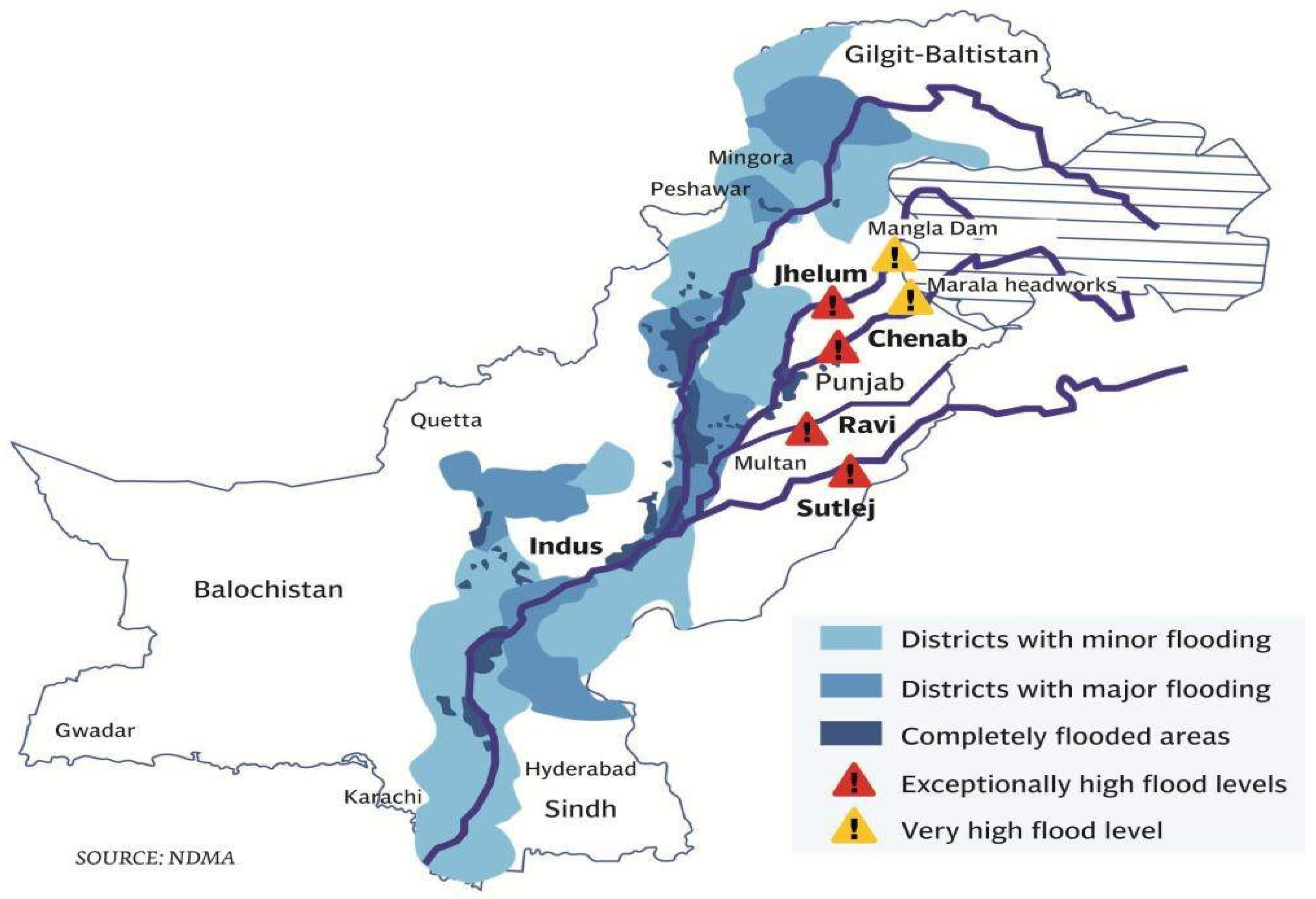
The Kashmir Valley is one of the most flood-prone regions in the world, located in the Greater Himalayas [11,12]. In the Kashmir Valley, the river Jhelum is the main river originating from the northwest portion of the Pir Panjal Mountain range. The Jhelum River enters Pakistan (Azad Kashmir) at Chakothi and flows through a narrow ravine toward the Mangla reservoir. In the past, the Jhelum River has had enormous flooding periodically, and among all the flood events, the flood in 1992 was the deadliest. The flood discharge measured downstream of the Rasul barrage was 952,170 cusecs, while the discharge carrying capacity of the Rasul barrage is approximately 850,000 cusecs. The flood caused the deaths of over 2000 people, including damage to various roads, bridges and infrastructure. Numerous agricultural lands and crops were also affected. Currently, Pakistan is facing severe flooding, but the Jhelum River is less inundated as compared to the Indus River. However, the Jhelum River is more prone to severe floods as it has previously had many severe flood events, including floods in 1992, 2010 and 2014. Figure 1 shows the flood-affected areas of Pakistan in 2014, including severe floods in the Jhelum River.
Previously, different studies have been conducted in the Jhelum River catchment in order to predict floods, streamflow and other hydrological parameters. Ref. [13] developed a model to predict precipitation and temperature in the Jhelum River catchment and utilized Artificial Neural Networks (ANN) and Multiple Linear Regression (MLR) techniques, although their model had less accuracy, i.e., for precipitation, the range of the coefficient of determination (R2) was 0.57–0.77. Ref. [14] developed a 2D rainfall–runoff model to simulate floods in the Jhelum River, however it had inadequate model accuracy, especially for the Rasul barrage, as the values of the coefficient of determination (R2) for peak flood and post-flood were 0.78 and 0.86, respectively. Similarly, ref. [15] conducted a study and developed a MIKE 11-NAM model for flood prediction in the Jhelum River basin at different stations. The model had limited accuracy, as depicted by performance indicators, including the coefficient of determination (R2). The values of R2 were in the range of 0.71–0.78 for calibration (2001–2008) and validation (2009–2014).
The flooding process is fundamentally complicated, questionable and erratic because of its nonlinear reliance on meteorological and topographical boundaries [16]. While distributed hydrological modeling involves multidisciplinary and complex issues, simple, robust and sustainable approaches in flood forecasting systems are needed. Different methodologies have been proposed for flood forecasting and can be partitioned into physically-based and data-driven techniques. Physically-based models are information based and expect to reproduce or mimic the entire hydrological processes to make forecasts. These models are complicated and require numerous boundaries connected with the basin area of interest and hence require expert opinion and impart limitations on the predictability and practicability of flood forecasting. Apart from these, data-driven models use mathematical and statistical equations in order to obtain realistic results. These sets of equations are applied to long time series data to predict different parameters such as dam inflow [17], water demand [18], streamflow [19], flood frequency [20], floods [5,6,21,22], dam failure [23] etc. Historical data plays a key role in data-driven models, which helps in providing flood extents such as runoff volume and flood depth.
The precise prediction of streamflow or flooding is an intricate task because of the nonlinear relationship between rainfall and runoff, both in spatial and temporal terms [24]. As mentioned above, the streamflow depends on different meteorological variables, which differ from time to time [25]. Different approaches for modeling have been employed; among them, physical modeling and data-driven modeling are more common [26]. The data-driven modeling, especially ANN and regression models, has created a revolution in the prediction of hydrometeorological parameters [25]. The application of artificial intelligence, specifically ANN, has gained popularity among stockholders as an accurate and efficient estimation tool for a variety of hydraulic, hydrologic and environmental details [27,28]. The main advantages of this acute approach over conventional modeling techniques are the ability to model the nonlinearity of hydrological variables and the ability to deal with a lot of information [29]. Examples of hydrologic parameter estimation using ANN includes streamflow [30]; reservoir levels [31,32]; sediment load in irrigation canal [33]; groundwater level prediction [34,35], rainfall–runoff modeling [36] and water quality prediction [37,38]. Studies have also reported that the ANN model performs well in tropical and sub-tropical climates [39]. Different ANN models have been utilized to predict the compression coefficient of soil [40]. Various researchers have successfully and effectively applied artificial neural networks (ANNs) for determining floods at various lead times [41,42,43,44]. There are a lot of studies related to flood forecasting using deep learning models such as Convolutional Neural Networks (CNN) and Recurrent Neural Networks (RNN) [45,46].
The ANN models show an expanded precision in flood anticipation regardless of the nonlinearity of the input information [47]. Additionally, flood anticipating precision is expanded because of higher lead times. One of the most important factors is that the accuracies of the forecasts do not rely upon the size of the river basin or the locale concerned, but rather, the patterns in the past data fed into the models [48]. Therefore, the greater performance of ANN models recommends that their use is preferred over conventional mathematical models. However, ref. [49] reported that ANN models might suffer due to the presence of nonlinearity in hydrological data, as the quality of data has a direct impact on the quality of learning maps in an ANN. Therefore, the quality of input data should be checked before using it as the input for data-driven models, specifically in ANN-based hydrological models. The checking of input data prior to data-driven modeling involves data preprocessing. Data preprocessing may include a process of input screening, which provides a set of inputs with less noise for our desired output.
Streamflow modeling plays an important role in water resource engineering and management as a flood early warning system. Numerous advanced models have been developed, but for a varying range of climatic regions; hence, a model suitable for local climatic conditions is needed. The hydrodynamic models have the ability to simulate a large range of flow conditions, but they need accurate river geometric data, which is not available for all locations. Therefore, this study provides a baseline to develop ANN- and regression-based models to estimate accurate discharges and streamflow in order to create an early flood warning system by alerting the areas downstream that are vulnerable to high water levels in the river. Hence, an early and timely evacuation of people along with minimum damage to infrastructure can be possible. Moreover, following the approach in this study, accurate streamflow predictions can be made in other flood-prone rivers.
2. Materials and Methods
2.1. Study Area and Dataset
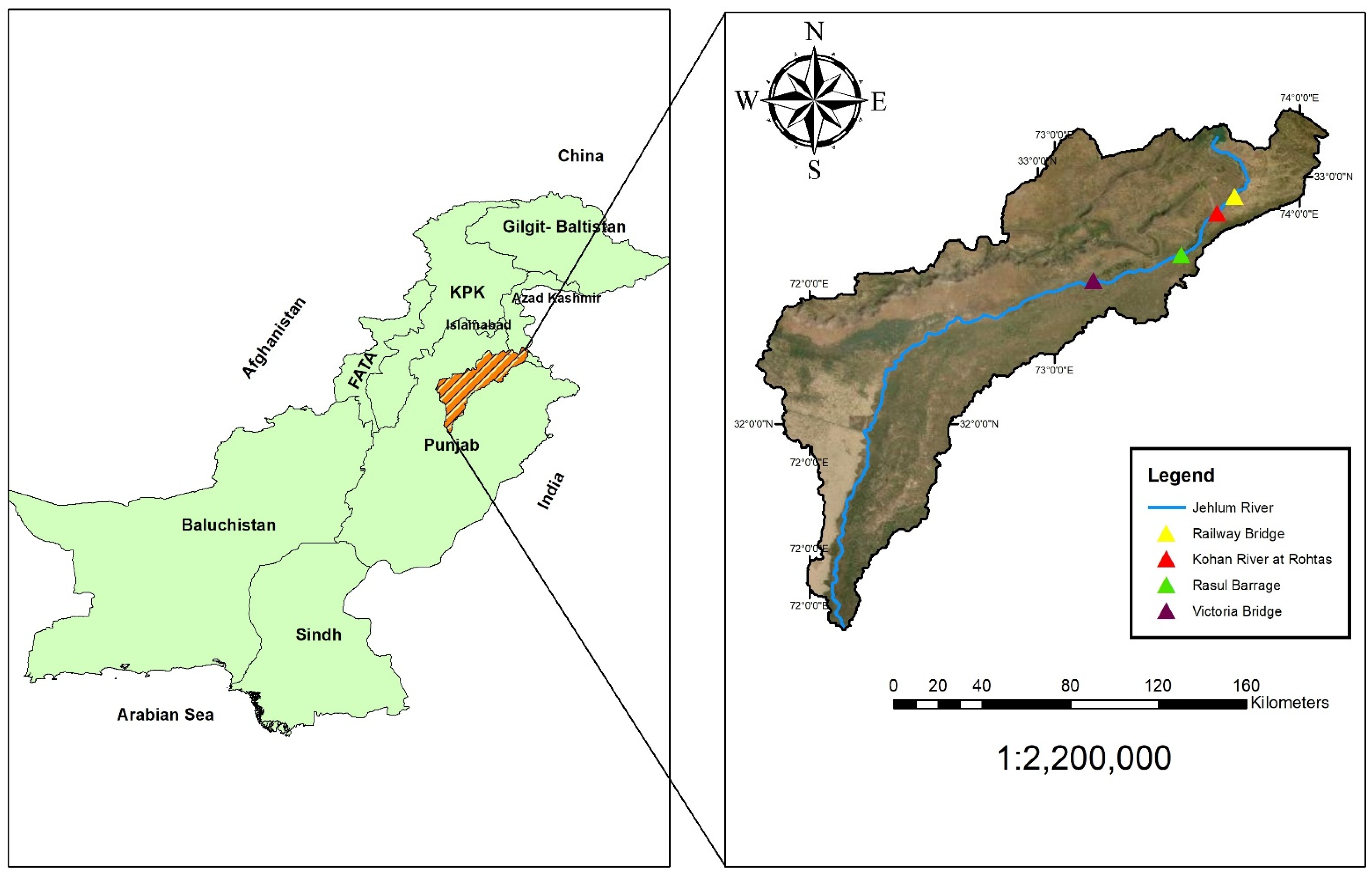
The Jhelum River, which is approximately 725 km long, originates from Jammu and Kashmir, through the Kashmir Valley, and flows into Pakistani Punjab. Geographically it lies in western Punjab, which is one of the tributaries of the Chenab River. There are a few dams and barrages constructed over the Jhelum River, including the Rasul barrage. The Barrage is located 72 km downstream of Mangla Dam and has a discharge capacity of approximately 24,070 cubic meters per second (approximately 850,000 cusecs). Four gauging stations were selected, including Railway Bridge, Rasul Barrage, Kohan River at Rohtas and Victoria Bridge. The first three stations were used as input, while the last station (Victoria Bridge) was used as the output. An advanced algorithm was used along with the ANN in order to train the model for the selected river by considering the antecedent condition of discharge. The study area along with location of different gauge stations is shown in Figure 2.
2.2. Datasets
Weekly observed data was collected from the Punjab Irrigation department for four stations. The datasets included the antecedent data condition of discharge of the gauging stations. For the model development, discharge at the following stations was taken as input: Railway Bridge, Rasul Barrage and Kohan River at Rohtas, while discharge at the Victoria Bridge was taken as output. Table 1 shows a detailed description of the datasets. The training and testing period was determined by the hit-and-trial method. From the data of 1256 vectors, 70% (885) vectors were considered for training, and the remaining 30% were considered for testing. The selection of the length of vectors was based on previous studies, ref. [50] considered 80% of the total data for training and 20% for testing.
2.3. Data Normalization
For Normalization, the data was first converted to a unitless quantity and then uniformly distributed through logarithmic transformation. Normalization was done as per Equation (1).
where:
Pi, Pmin, Pmax are the ith value of P, minimum value of P, and maximum value of P, respectively.
2.4. Input Combination Selection Using Gamma Test and Advanced Model Identification Techniques
Feature selection assists with understanding the data, improving the performance in prediction, and reducing the requirement of computation [51]. The Gamma test is an advanced tool that has been utilized for estimation in various areas, including the selection of features [52], communications [53], control theory [54], sediment transport [33], along with hydrological modeling [55,56,57,58].
By capturing the intricate relationships among different outputs and inputs, the Gamma test estimates the mean square error (MSE). A specific output (y) is the function of the specific input (x) as defined by the algorithm in the Gamma test.
The function is divided into two separate parts, known as the smooth part and the function carrying the noise in the data. Considering f is the function containing the smooth part, while r is the part of an output that cannot be reflected in the development of a smooth model, then the relationship between y and x can be described by Equation (2) [59]. The average value of r is presumed to be zero by allocating a constant error to the function (f), which is not known. Although f is not known, the Gamma test allows us to predict the r value in some circumstances. With an increase in the number of observations, the Gamma value equals a value that is asymptotic and represents the variance of noise in the output [59].
Hence, the Gamma test enables us to predict the part of the output variance that the smooth data model is unable to calculate. Moreover, it has been shown, based on experiments, that the results predicted by the Gamma test are more accurate than other methods, such as the Mutual Information (MI) method [60]. The model identification techniques enable us to develop the input combinations efficiently by utilizing advanced algorithms. Different model identification techniques have been used previously, including Genetic Algorithm (GA) by [49,61] for the forecasting of streamflow. Similarly, [33] employed GA, Hill Climbing (HC), Full Embedding (FE), Increasing Embedding (IE) and Sequential Embedding (SE) for sediment load prediction in an irrigation canal.
The Gamma test calculates the MSE value for each set of input combinations. Whichever combination provides the least value is selected as the best combination for desirable outputs that are smooth and noise free.
where:
P = F(q) + R
P is a function of q, F is the smooth model and R is noise. Taking the R component as 0 from Equation (2) a constant bias associated with our function F.
Total 2n−1 combinations are possible in the Gamma test, which creates a tedious task where unwanted input combinations will be formed. To overcome this problem, the win Gamma environment was used in order to identify the best possible combinations that will lead to reliable and realistic results.
2.5. Model Development
2.5.1. Local Linear Regression (LLR)
Local Linear Regression is widely used for forecasting due to its accuracy and high degree of precision. In this method, the nearest neighbors have to be selected, which is necessarily required for matrix calculation.
where:
X is the d matrix with the input points Pmax in the d dimension, which indicates nearest neighbor points, y indicates the column vector with a length equal to Pmax, and m is a column vector of the parameters that are the outputs of the matrix calculations.
2.5.2. Dynamic Local Linear Regression (DLLR)
Dynamic Local Linear Regression (DLLR) is a modeling approach that is identical to LLR and has surplus features in a way that when data is incorporated, new data is observed in the model. When new data is incorporated into the model (after attempting the prediction stage), the DLLR model performs and predicts better [62]. The effect can be seen if the model is started with a small training dataset and a large testing dataset. It is recommended to start the DLLR model with a training dataset of reasonable size, as the initial kd-tree will be better balanced, and there will be a reduction in query times. The DLLR is simply an LLR model with dynamic updates and is good for use in time series prediction.
2.5.3. Artificial Neural Networks (ANNs)
The concept of ANN is very similar to our neuron system. As neurons are connected with each other by nodes, similarly ANN is also a collective group of nodes. The function of ANN is very similar to how our neurons work, the output from one node is input for another node. As connected nodes receive the signal, they are multiplied with corresponding weights, and finally, these signals are added for a particular junction. Supervised and unsupervised are two learning methodologies; among these two, supervised learning is widely used. In supervised learning, input and output need to be added into the network in order to change the weights with the objective of minimizing error in the final output product. ANN has an input layer and an output layer, where the input layer can have more than one layer; therefore, the layers between the first and last layer (output layer) are called intermediate layers [63].
In this study, we considered three Artificial Neural Network-based methods, namely Two Layer Back Propagation (TLBP), Broyden–Fletcher–Goldfarb–Shanno (BFGS) and Conjugate Gradient Neural Network (CGNN) [64]. The structure of ANN models was optimized by changing the number of nodes in hidden layers of a multi-layer neuron network. However, the number of hidden layers was fixed as two (02) due to their capability of capturing the complex and nonlinear behavior of streams. Previously, the two hidden layers have been successfully used by [49] to train ANN-based streamflow estimation models [33] for sediment load estimation models, and for the estimation of reservoir levels [32]. Although there are some rules of thumb for the selection of number of nodes in hidden layers, ref. [65] reported that the best practice to optimize the number of nodes in hidden layers is to “try” and “evaluate” them on the basis of model performance. The same approach has been adopted in this case, by trying and evaluating the number of nodes in each hidden layer on the basis of the MSE (Gamma Value) achieved. The three best trails to optimize the ANN architecture of each ANN technique (TLBP, BFGS and CGNN) are shown in Table 2. A comparison was made between the efficiency of the ANN-based model, Local Linear Regression (LLR) and Dynamic Local Linear Regression (DLLR) models. The most efficient model was identified by statistical performance evaluation matrices namely root mean square error (RMSE), variance, bias, coefficient of determination (R2) and mean squared error (MSE).
3. Results
3.1. Gamma Test Results
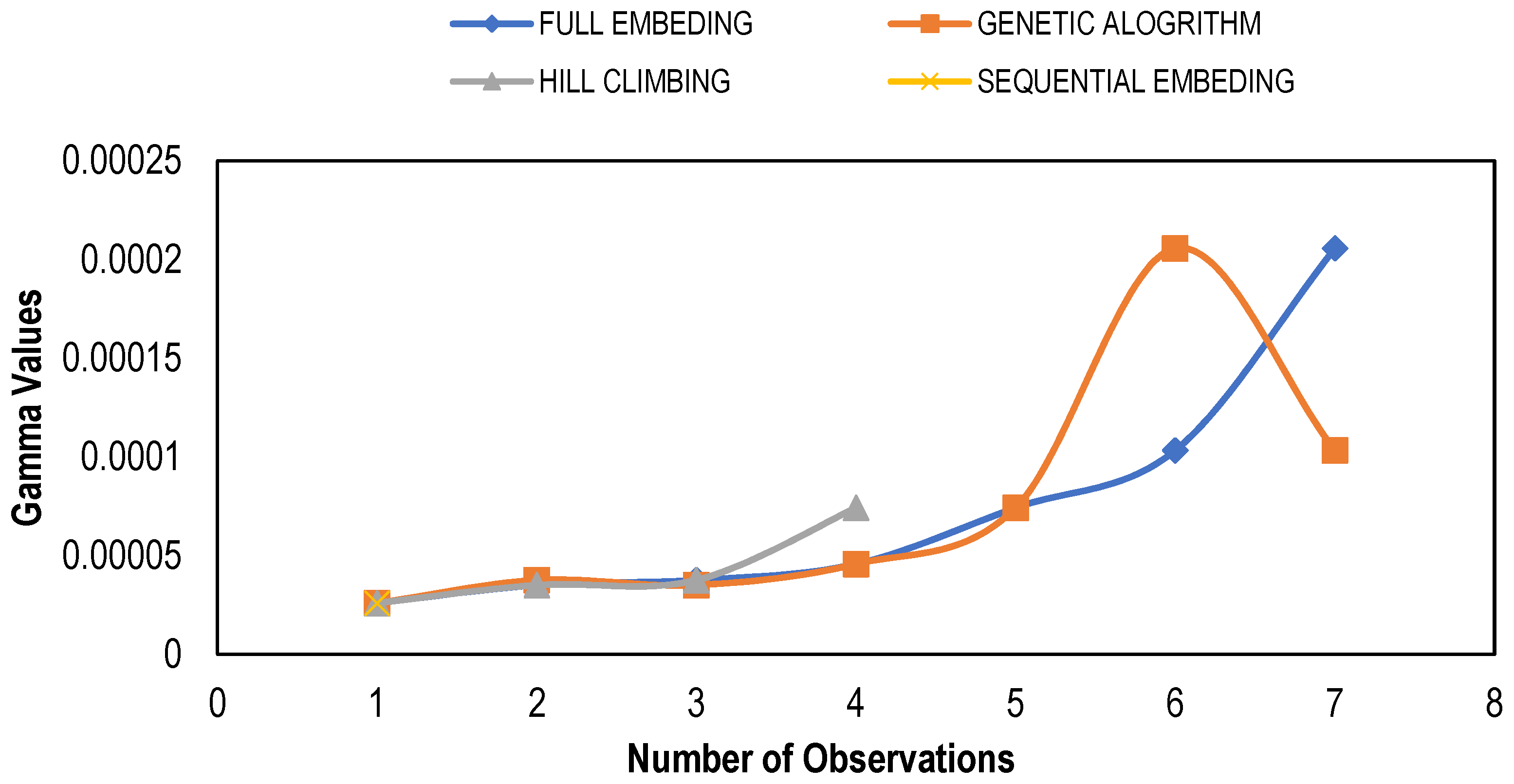
Figure 3 shows the graph between the variation in Gamma values for different combinations/masks determined through multiple feature selection techniques. The figure shows that almost all the feature selection methods showed low Gamma values for similar mask inputs, which are 001 and 111. The “0” shows that the input is excluded, whereas the “1” depicts the inclusion of a particular input. The best mask based on the minimum Gamma value for each technique with gradient, standard error and V ratios is listed in Table 3. For model development, the input combinations with minimum Gamma values were selected. This Gamma value was used as a targeted MSE to train the ANN and Regression models by using the respective set of input combinations. It can be seen that among all modeling techniques, the Genetic Algorithm (GA) and Hill Climbing (HC) techniques had minimum Gamma values, while Full Embedding (FE) had the maximum. It is also clear that along with low Gamma values, the gradient and V ratio are also less for GA and HC.
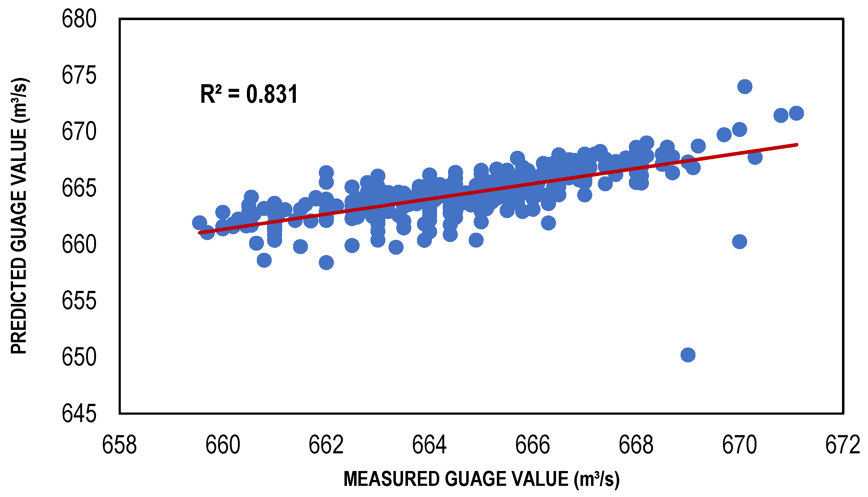
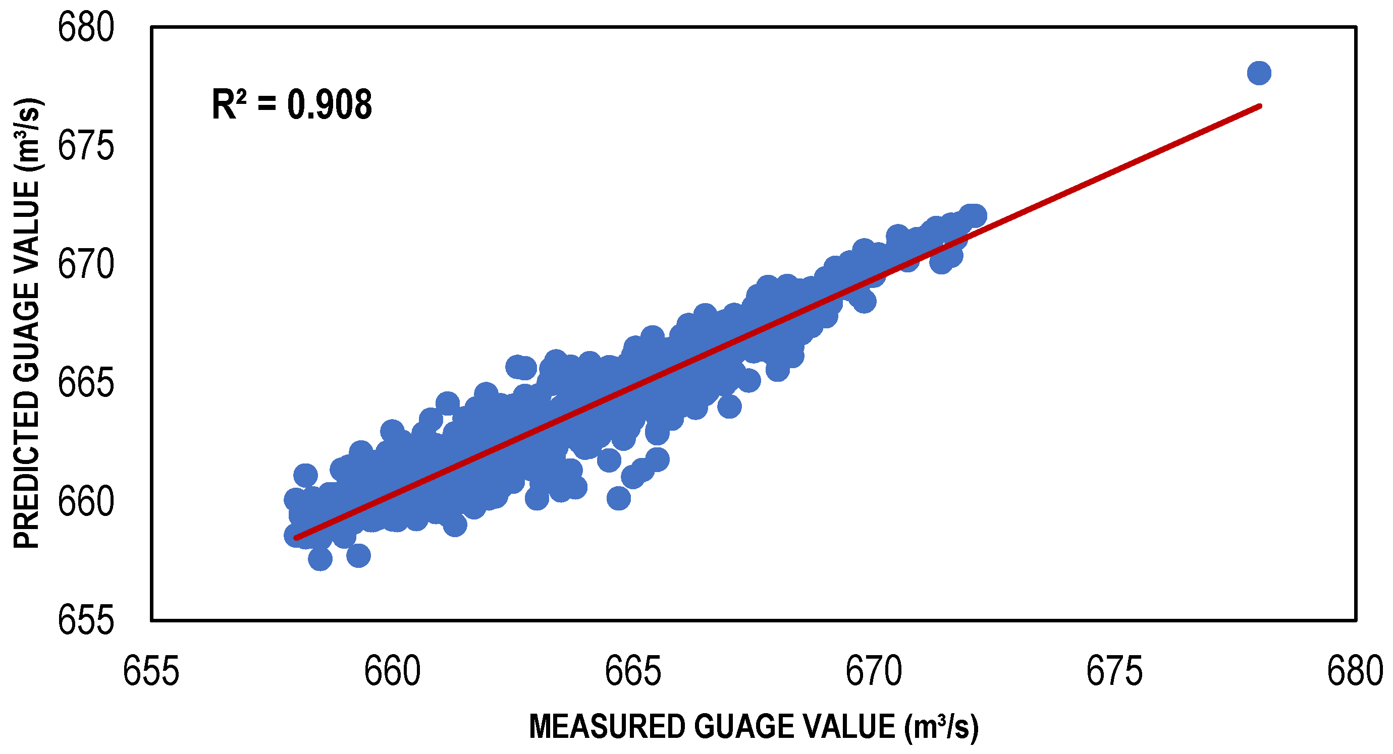
3.2. LLR and DLLR Results
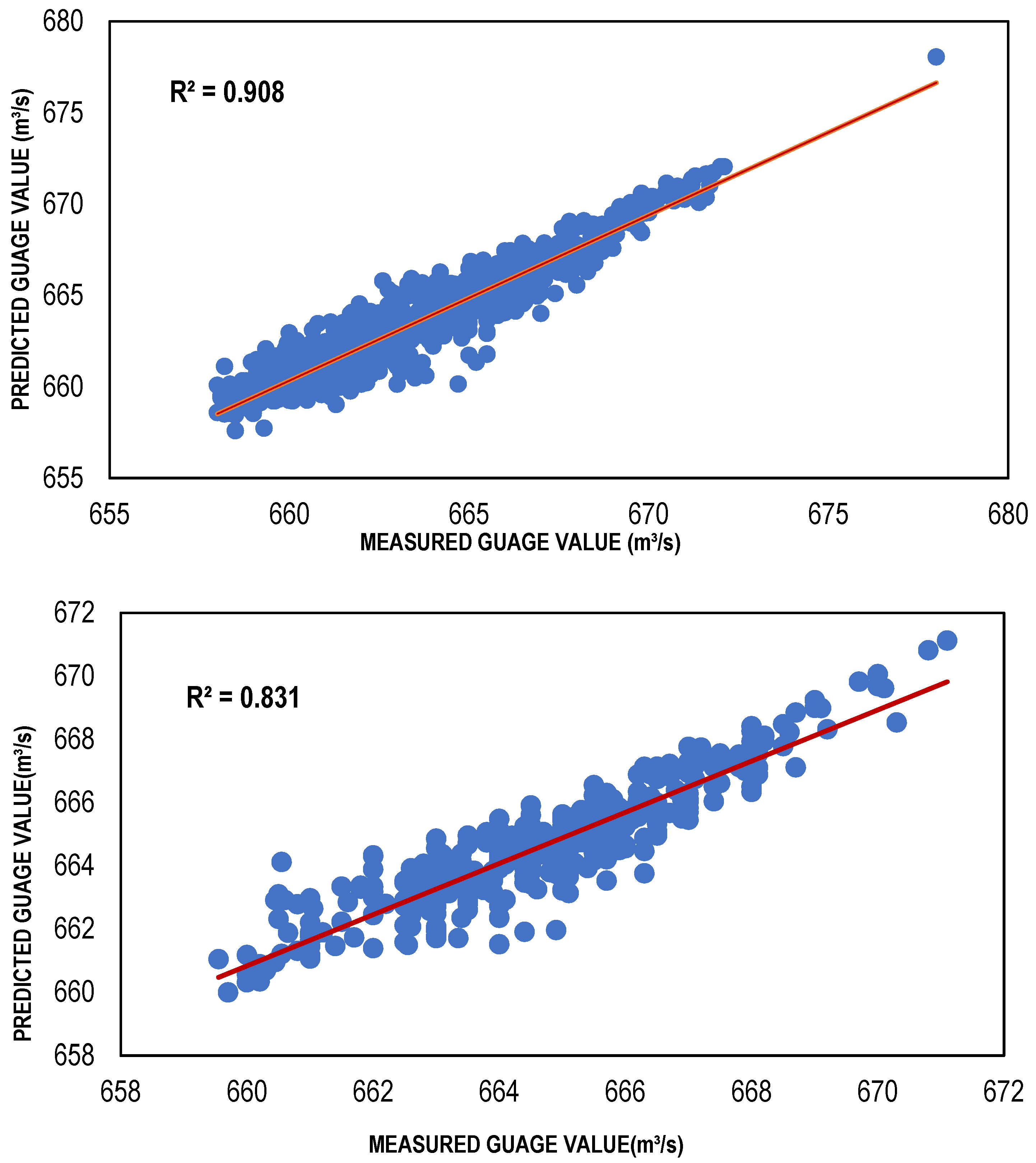
The Local Linear Regression (LLR) models were developed for a different set of input combinations, which were determined through multiple feature selection techniques. For the training of LLR models, 10 nearest neighbors were considered to classify the given data points. [66] conducted a study and found that selection of 10 to 20 nearest neighbors was best suitable for a small length of data as for the data of larger length, the number of nearest neighbors should be augmented for a precise solution. The results in the form of performance indicators (Table 4) showed that LLR and DLLR performed well with reasonably high values of R2 = (Train, Test) 0.91, 0.83 and 0.91 and 0.83, and low values of Bias = (Train, Test) 0.009, −0.053 and −0.01 and −0.017, respectively. The same models showed very low values of RMSE for LLR and DLLR in both the training and testing phases. Both the LLR and DLLR models performed well for the input combination (001) determined through GA, despite the fact that it has relatively large values of Gamma as compared to the other feature selection techniques. The reason LLR and DLLR performed well with this combination is that it considered only one input which is the discharge of the Jhelum River located just upstream of the desired point/station, where the estimation models were developed. The simple and linear nature of regression models exhibited better predictive power with a smaller number of inputs as compared to the ANN-based estimation models. Such models are often called parsimonious models because they have the capacity of performing well with their simple nature and great predictive power [67]. The scatter plots showing both the training and testing data for the best LLR and DLLR models are presented in Figure 4 and Figure 5.
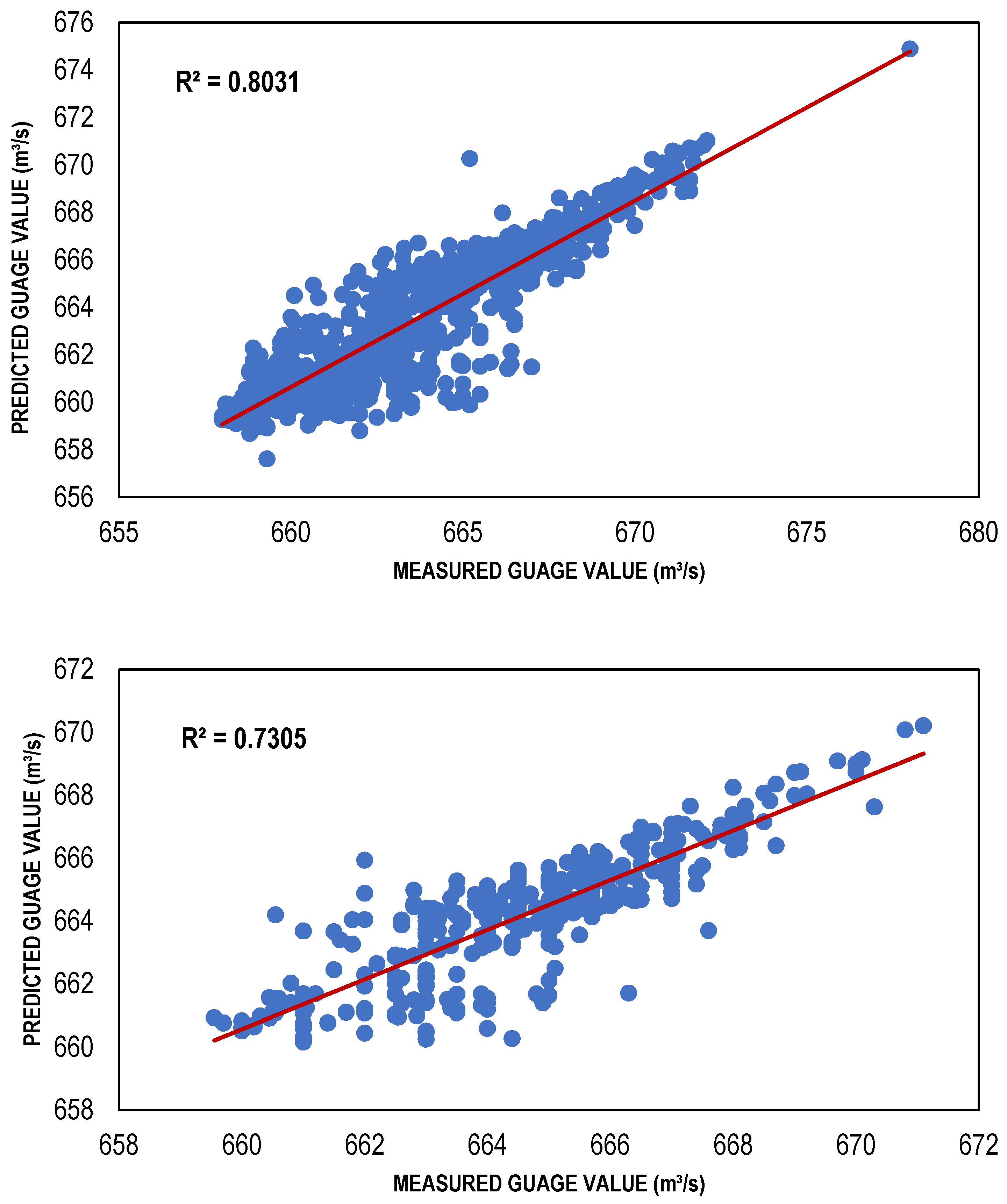
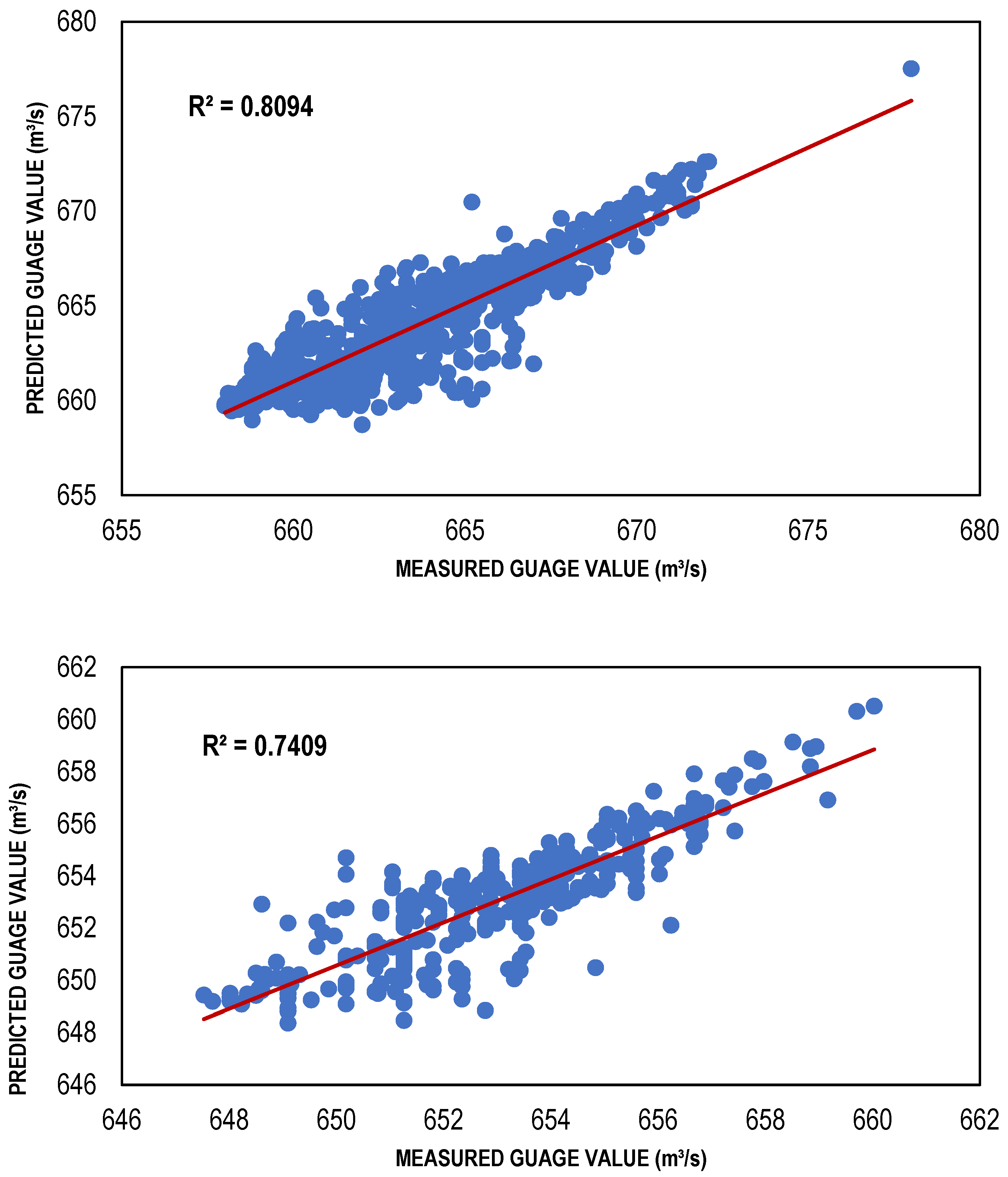
3.3. ANN Results
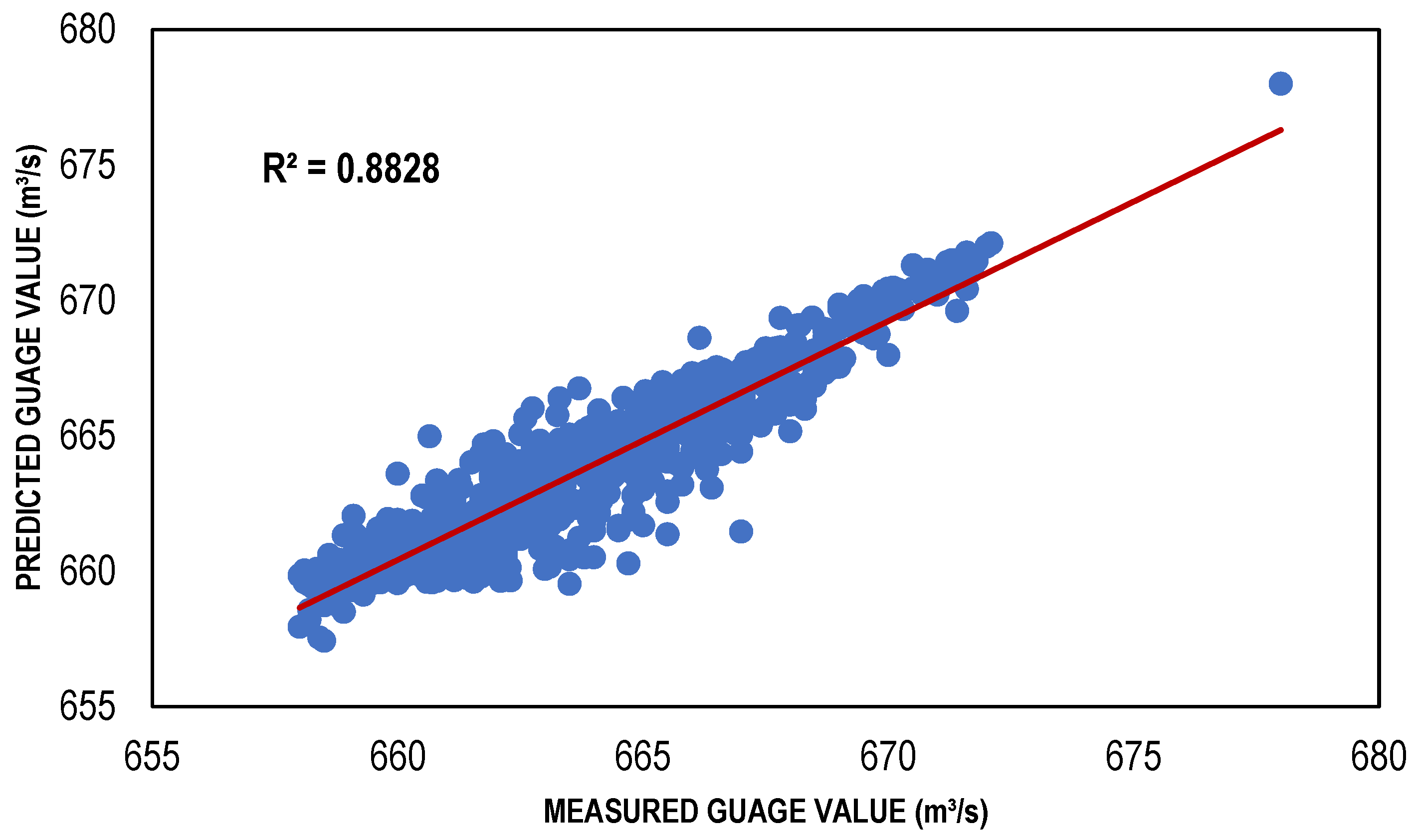
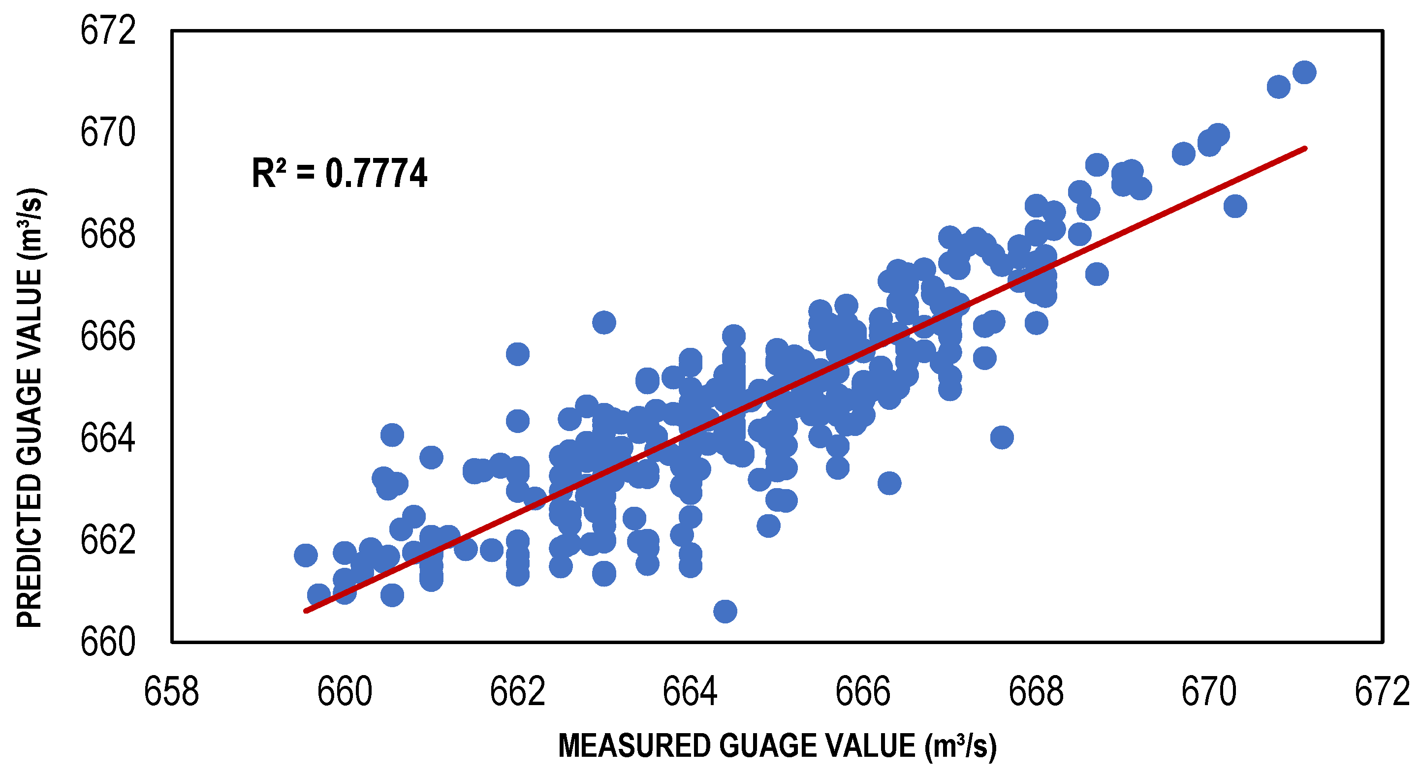
The ANN-based streamflow estimation models were trained via TLBP, CGNN and BFGS algorithms using Gamma value as a targeted MSE for different input masks, determined through GA, HC, FE, Sequential Embedding (SE) and Increasing Embedding (IE). Table 4 shows the values of performance indicators, including R2, RMSE and bias for all types of ANN models developed for the masks determined through GA, HC, SE and IE because the models developed for these combinations performed better as compared to the models developed for masks through GA and FE. It is clear from that table that ANN models showed reasonably high values of R2; for TLBP = 0.80, 0.73; CGNN = 0.81, 0.74; and BFGS = 0.88, 0.78; in both training and testing phases. Similarly, the values of bias and RMSE are also less for these models showing their capacity to perform well with reasonable accuracy. Although, the ANN models have lower performance than regression models based on the performance indicators. However, among the ANN models, the performance of the BFGS model was best as compared to other ANN models with maximum R2 values (0.8828 and 0.7774) and minimum RMSE values (1.149249 and 1.052597); whereas TLBP had minimum R2 values (0.8031 and 0.7305) and maximum RMSE values (1.493783 and 1.238525) in both training and testing phases, respectively. The BFGS model outperformed other ANN models because it is a quasi-Newton-based approach and employment of a method of iteration that is relatively effective for the solution of nonlinear problems.

Table 4.
Comparison of selected input combinations (training and testing).
| Model | Training | |||
|---|---|---|---|---|
| Mask | R sq. | Bias | RMSE | |
| LLR model | 001 | 0.908 | 0.009205 | 1.018017 |
| DLLR model | 001 | 0.908 | −0.01095 | 1.008635 |
| TLBP-based ANN model | 111 | 0.8031 | −0.09179 | 1.493783 |
| CG-based ANN model | 111 | 0.8094 | 0.401287 | 1.520267 |
| BFGS-based ANN model | 111 | 0.8828 | 0.012462 | 1.149249 |
| Model | Testing | |||
| Mask | R sq. | Bias | RMSE | |
| LLR model | 001 | 0.831 | −0.05344 | 0.919695 |
| DLLR model | 001 | 0.831 | −0.16991 | 1.766721 |
| TLBP-based ANN model | 111 | 0.7305 | −0.4131 | 1.238525 |
| CG-based ANN model | 111 | 0.7409 | 0.036029 | 1.251868 |
| BFGS-based ANN model | 111 | 0.7774 | −0.03043 | 1.052597 |
4. Comparison and Discussion
Scatter plots of the training and testing of LLR and DLLR models are shown in Figure 4 and Figure 5 whereas for ANN models they are shown in the Figure 6, Figure 7 and Figure 8. For comparing different models’ various performance evaluation matrices, such as mean square error (MSE), model efficiency (R2) and root mean square (RMSE) were utilized. The LLR and DLLR outperformed other models with high values of R2, 0.908 in training and 0.831 in testing, respectively. Moreover, the regression models performed well as compared to other models with a minimum RMSE in the case of LLR for training = 1.018017 and testing = 0.919695, respectively, while in the case of DLLR, it came out to be 1.008635 for training and 1.766721 for testing, respectively. The reason behind the better performance of the regression-based models as compared to the ANN models is due to their parsimonious behavior for the mask of inputs (001), which has the least number of input(s). For this mask (FE), the targeted MSE value is high (0.00021) as compared to the Gamma values for other masks of inputs (HC, SE and IE), which contain more inputs (111). Therefore, regression-based linear models, including LLR and DLLR, performed well for this combination of inputs by easily achieving the targeted MSE with only one input for the mask (001). On the other hand, the ANN-based models targeted the combination/mask (111) with the least Gamma values, but a greater number of inputs. Thus, remained unable to perform as well as the regression-based models due to the greater complexity involved. Similarly, the gradient-based ANN algorithms, including BFGS and CGNN, are quite fast, but they are often stuck at local minima and sometimes failed to achieve optimum results [68]. However, the models developed using both ANN and regression could be used for the streamflow estimation in the region with reasonable accuracy. In the present case, the use of the Gamma test was found to be more advantageous for regression-based streamflow estimation models as compared to the ANN-based flow estimation models.
Previously, the upper Indus Basin (UIB) has been the key area of climate and hydrological studies, as many researchers have performed hydrological and climate modeling on the upper part of the Indus basin [49,69,70]. However, the Jhelum catchment was neglected despite its previous history of flooding and the need for water management in the region. Only a few studies have been carried out so far, e.g., [15,71]. These studies have low-performance indicators for streamflow estimation in the region [13,14,15] as compared to the present study. Therefore, the current model can provide a quick, flexible and time-saving approach for flood forecasting in the Jhelum River. The study can provide a baseline for the development of an early flood warning system for the used river sections of the Jhelum River. For the flood disaster of 1992, 2010 and 2014 in Jhelum River Pakistan, the predicted readings of the current model should be compared with the actual readings in order to better evaluate the model performance. Furthermore, future studies should focus on the real-time application of the model, as the current study is limited only to time series hydrological modeling.
5. Summary & Conclusions
This study compares different AI techniques to predict floods in the Jhelum River of the region of Punjab (Pakistan). First, the best input combination was decided for modeling, where the regression models had the mask (001), and the ANN models had the mask (111). The LLR and ANN models were then developed, trained, and tested. The performances of these models were mainly analyzed by R2, bias, and RMSE. The final selection of the model was based on the overall performance of the model.
The observations concluded that the LLR model performed best among all. It can be concluded that the LLR model can be used for the prediction of flood in the selected study area, however it is not necessarily valid for other regions due to geological and climatological variations. The study revealed that for flood prediction, regression models can be utilized with a high degree of precision at the current location of study in the Jhelum River. It was also found that the Gamma test could be employed to decide the best input combination in order to develop smooth ANN and regression models.
It is recommended that further studies should be carried out as the incorporation of more temporally finer resolution data leads to more reliable results. Moreover, this study can be extended by incorporating other AI models that may provide more suitable outputs.
Author Contributions
Conceptualization, H.H.L. and F.A.; methodology, F.A.; software, F.A. and M.H.; validation, E.P., M.H. and P.J.; formal analysis, F.A. and M.H.; investigation, F.A.; resources, E.P. and P.J.; data curation, F.A.; writing—original draft preparation, F.A.; writing—review and editing, H.H.L., E.P., M.H. and P.J.; visualization, F.A. and M.H.; supervision, H.H.L.; project administration, H.H.L.; funding acquisition, E.P. All authors have read and agreed to the published version of the manuscript.
Funding
This research was funded by the Ministry of Education of Singapore (#Tier1 2021-T1-001-056 and #Tier2 MOE-T2EP402A20-0001).
Institutional Review Board Statement
Not applicable.
Informed Consent Statement
Not applicable.
Data Availability Statement
Data will be made available on request.
Acknowledgments
The authors would like to acknowledge the Punjab Irrigation department, Pakistan for providing the discharge data used in this study.
Conflicts of Interest
The authors declare no conflict of interest.
References
- Sapitang, M.; Ridwan, W.M.; Kushiar, K.F.; Ahmed, A.N.; El-Shafie, A. Machine Learning Application in Reservoir Water Level Forecasting for Sustainable Hydropower Generation Strategy. Sustainability 2020, 12, 6121. [Google Scholar] [CrossRef]
- Berz, G. Flood Disasters: Lessons from the Past—Worries for the Future. Proc. Inst. Civ. Eng. —Water Marit. Eng. 2000, 142, 3–8. [Google Scholar] [CrossRef]
- Arduino, G.; Reggiani, P.; Todini, E. Recent Advances in Flood Forecasting and Flood Risk Assessment. Hydrol. Earth Syst. Sci. 2005, 9, 280–284. [Google Scholar] [CrossRef] [Green Version]
- Courtney, C. The Nature of Disaster in China: The 1931 Yangzi River Flood; Cambridge University Press: Cambridge, UK, 2018; ISBN 9781108278362. [Google Scholar]
- Loc, H.H.; Park, E.; Chitwatkulsiri, D.; Lim, J.; Yun, S.-H.; Maneechot, L.; Minh Phuong, D. Local Rainfall or River Overflow? Re-Evaluating the Cause of the Great 2011 Thailand Flood. J. Hydrol. 2020, 589, 125368. [Google Scholar] [CrossRef]
- Loc, H.H.; Emadzadeh, A.; Park, E.; Nontikansak, P.; Deo, R.C. The Great 2011 Thailand Flood Disaster Revisited: Could It Have Been Mitigated by Different Dam Operations Based on Better Weather Forecasts? Environ. Res. 2023, 216, 114493. [Google Scholar] [CrossRef] [PubMed]
- Kala, C.P. Deluge, Disaster and Development in Uttarakhand Himalayan Region of India: Challenges and Lessons for Disaster Management. Int. J. Disaster Risk Reduct. 2014, 8, 143–152. [Google Scholar] [CrossRef]
- Shah, S.M.H.; Mustaffa, Z.; Teo, F.Y.; Imam, M.A.H.; Yusof, K.W.; Al-Qadami, E.H.H. A Review of the Flood Hazard and Risk Management in the South Asian Region, Particularly Pakistan. Sci. Afr. 2020, 10, e00651. [Google Scholar] [CrossRef]
- Ghatak, M.; Ahmed; Mishra, O.P. Background Paper on Flood Risk Management in South Asia. In Proceedings of the SAARC Workshop on Flood Risk Management in South Asia, Islamabad, Pakistan, 9–10 October 2012. [Google Scholar]
- Ministry of Water Resources, Government of Pakistan. Federal Flood Commission Report; Ministry of Water Resources, Government of Pakistan: Islamabad, Pakistan, 2018. [Google Scholar]
- Sen, D. Flood Hazards in India and Management Strategies. In Natural and Anthropogenic Disasters; Springer: Dordrecht, The Netherlands, 2010; pp. 126–146. [Google Scholar]
- Altaf, F.; Meraj, G.; Romshoo, S.A. Morphometric Analysis to Infer Hydrological Behaviour of Lidder Watershed, Western Himalaya, India. Geogr. J. 2013, 2013, 1–14. [Google Scholar] [CrossRef] [Green Version]
- Akhter, M.; Manzoor Ahmad, A. Climate Modeling of Jhelum River Basin-A Comparative Study. Environ. Pollut. Clim. Change 2017, 1, 1–14. [Google Scholar] [CrossRef] [Green Version]
- Siddiqui, M.J.; Haider, S.; Gabriel, H.F.; Shahzad, A. Rainfall–Runoff, Flood Inundation and Sensitivity Analysis of the 2014 Pakistan Flood in the Jhelum and Chenab River Basin. Hydrol. Sci. J. 2018, 63, 1976–1997. [Google Scholar] [CrossRef]
- Parvaze, S.; Khan, J.N.; Kumar, R.; Allaie, S.P. Flood Forecasting in Jhelum River Basin Using Integrated Hydrological and Hydraulic Modeling Approach with a Real-Time Updating Procedure. Clim. Dyn. 2022, 59, 2231–2255. [Google Scholar] [CrossRef]
- Thirumalaiah, K.; Deo, M.C. Real-Time Flood Forecasting Using Neural Networks. Comput. -Aided Civ. Infrastruct. Eng. 1998, 13, 101–111. [Google Scholar] [CrossRef]
- Valipour, M.; Banihabib, M.E.; Behbahani, S.M.R. Comparison of the ARMA, ARIMA, and the Autoregressive Artificial Neural Network Models in Forecasting the Monthly Inflow of Dez Dam Reservoir. J. Hydrol. 2013, 476, 433–441. [Google Scholar] [CrossRef]
- Adamowski, J.; Fung Chan, H.; Prasher, S.O.; Ozga-Zielinski, B.; Sliusarieva, A. Comparison of Multiple Linear and Nonlinear Regression, Autoregressive Integrated Moving Average, Artificial Neural Network, and Wavelet Artificial Neural Network Methods for Urban Water Demand Forecasting in Montreal, Canada. Water Resour. Res. 2012, 48. [Google Scholar] [CrossRef]
- Wu, C.L.; Chau, K.W.; Li, Y.S. Predicting Monthly Streamflow Using Data-Driven Models Coupled with Data-Preprocessing Techniques. Water Resour. Res. 2009, 45. [Google Scholar] [CrossRef] [Green Version]
- Park, E.; Ho, H.L.; Tran, D.D.; Yang, X.; Alcantara, E.; Merino, E.; Son, V.H. Dramatic Decrease of Flood Frequency in the Mekong Delta Due to River-Bed Mining and Dyke Construction. Sci. Total Environ. 2020, 723, 138066. [Google Scholar] [CrossRef]
- Qiu, J.; Cao, B.; Park, E.; Yang, X.; Zhang, W.; Tarolli, P. Flood Monitoring in Rural Areas of the Pearl River Basin (China) Using Sentinel-1 SAR. Remote Sens. 2021, 13, 1384. [Google Scholar] [CrossRef]
- Chitwatkulsiri, D.; Miyamoto, H.; Irvine, K.N.; Pilailar, S.; Loc, H.H. Development and Application of a Real-Time Flood Forecasting System (RTFlood System) in a Tropical Urban Area: A Case Study of Ramkhamhaeng Polder, Bangkok, Thailand. Water 2022, 14, 1641. [Google Scholar] [CrossRef]
- Latrubesse, E.M.; Park, E.; Sieh, K.; Dang, T.; Lin, Y.N.; Yun, S.-H. Dam Failure and a Catastrophic Flood in the Mekong Basin (Bolaven Plateau), Southern Laos, 2018. Geomorphology 2020, 362, 107221. [Google Scholar] [CrossRef]
- Cluckie, I.D.; Han, D. Fluvial Flood Forecasting. Water Environ. J. 2000, 14, 270–276. [Google Scholar] [CrossRef]
- Remesan, R.; Ahmadi, A.; Shamim, M.A.; Han, D. Effect of Data Time Interval on Real-Time Flood Forecasting. J. Hydroinformatics 2010, 12, 396–407. [Google Scholar] [CrossRef]
- Wang, W. Stochasticity, Nonlinearity and Forecasting of Streamflow Processes; IOS Press: Amsterdam, The Netherlands, 2006. [Google Scholar]
- Tsai, W.-P.; Chang, F.-J.; Chang, L.-C.; Herricks, E.E. AI Techniques for Optimizing Multi-Objective Reservoir Operation upon Human and Riverine Ecosystem Demands. J. Hydrol. 2015, 530, 634–644. [Google Scholar] [CrossRef]
- Chang, F.-J.; Tsai, M.-J. A Nonlinear Spatio-Temporal Lumping of Radar Rainfall for Modeling Multi-Step-Ahead Inflow Forecasts by Data-Driven Techniques. J. Hydrol. 2016, 535, 256–269. [Google Scholar] [CrossRef]
- Nayak, P.C.; Sudheer, K.P.; Ramasastri, K.S. Fuzzy Computing Based Rainfall-Runoff Model for Real Time Flood Forecasting. Hydrol. Process. 2005, 19, 955–968. [Google Scholar] [CrossRef]
- Hassan, Z.; Shamsudin, S.; Harun, S.; Malek, M.A.; Hamidon, N. Suitability of ANN Applied as a Hydrological Model Coupled with Statistical Downscaling Model: A Case Study in the Northern Area of Peninsular Malaysia. Environ. Earth Sci. 2015, 74, 463–477. [Google Scholar] [CrossRef] [Green Version]
- Shamim, M.A.; Bray, M.; Remesan, R.; Han, D. A Hybrid Modelling Approach for Assessing Solar Radiation. Theor. Appl. Climatol. 2015, 122, 403–420. [Google Scholar] [CrossRef]
- Shamim, M.A.; Hassan, M.; Ahmad, S.; Zeeshan, M. A Comparison of Artificial Neural Networks (ANN) and Local Linear Regression (LLR) Techniques for Predicting Monthly Reservoir Levels. KSCE J. Civ. Eng. 2016, 20, 971–977. [Google Scholar] [CrossRef]
- Ahmed, F.; Hassan, M.; Hashmi, H.N. Developing Nonlinear Models for Sediment Load Estimation in an Irrigation Canal. Acta Geophys. 2018, 66, 1485–1494. [Google Scholar] [CrossRef]
- Lee, S.; Lee, K.-K.; Yoon, H. Using Artificial Neural Network Models for Groundwater Level Forecasting and Assessment of the Relative Impacts of Influencing Factors. Hydrogeol. J. 2019, 27, 567–579. [Google Scholar] [CrossRef]
- Wunsch, A.; Liesch, T.; Broda, S. Forecasting Groundwater Levels Using Nonlinear Autoregressive Networks with Exogenous Input (NARX). J. Hydrol. 2018, 567, 743–758. [Google Scholar] [CrossRef]
- Van, S.P.; Le, H.M.; Thanh, D.V.; Dang, T.D.; Loc, H.H.; Anh, D.T. Deep Learning Convolutional Neural Network in Rainfall–Runoff Modelling. J. Hydroinformatics 2020, 22, 541–561. [Google Scholar] [CrossRef] [Green Version]
- Ahmed, U.; Mumtaz, R.; Anwar, H.; Shah, A.A.; Irfan, R.; García-Nieto, J. Efficient Water Quality Prediction Using Supervised Machine Learning. Water 2019, 11, 2210. [Google Scholar] [CrossRef] [Green Version]
- Loc, H.H.; Do, Q.H.; Cokro, A.A.; Irvine, K.N. Deep Neural Network Analyses of Water Quality Time Series Associated with Water Sensitive Urban Design (WSUD) Features. J. Appl. Water Eng. Res. 2020, 8, 313–332. [Google Scholar] [CrossRef]
- Pradhan, P.; Kriewald, S.; Costa, L.; Rybski, D.; Benton, T.G.; Fischer, G.; Kropp, J.P. Urban Food Systems: How Regionalization Can Contribute to Climate Change Mitigation. Environ. Sci. Technol. 2020, 54, 10551–10560. [Google Scholar] [CrossRef] [PubMed]
- Pham, B.T.; Nguyen, M.D.; van Dao, D.; Prakash, I.; Ly, H.-B.; Le, T.-T.; Ho, L.S.; Nguyen, K.T.; Ngo, T.Q.; Hoang, V.; et al. Development of Artificial Intelligence Models for the Prediction of Compression Coefficient of Soil: An Application of Monte Carlo Sensitivity Analysis. Sci. Total Environ. 2019, 679, 172–184. [Google Scholar] [CrossRef]
- DAWSON, C.W.; WILBY, R. An Artificial Neural Network Approach to Rainfall-Runoff Modelling. Hydrol. Sci. J. 1998, 43, 47–66. [Google Scholar] [CrossRef]
- Sudheer, K.P.; Gosain, A.K.; Ramasastri, K.S. A Data-Driven Algorithm for Constructing Artificial Neural Network Rainfall-Runoff Models. Hydrol. Process. 2002, 16, 1325–1330. [Google Scholar] [CrossRef]
- Sudheer, K.P. Knowledge Extraction from Trained Neural Network River Flow Models. J. Hydrol. Eng. 2005, 10, 264–269. [Google Scholar] [CrossRef]
- CHANG, F.-J.; CHIANG, Y.-M.; CHANG, L.-C. Multi-Step-Ahead Neural Networks for Flood Forecasting. Hydrol. Sci. J. 2007, 52, 114–130. [Google Scholar] [CrossRef]
- Padmawar, P.M.; Shinde, A.S.; Sayyed, T.Z.; Shinde, S.K.; Moholkar, K. Disaster Prediction System Using Convolution Neural Network. In Proceedings of the 2019 IEEE International Conference on Communication and Electronics Systems (ICCES), Coimbatore, India, 17–19 July 2019; pp. 808–812. [Google Scholar]
- Li, W.; Kiaghadi, A.; Dawson, C. Exploring the Best Sequence LSTM Modeling Architecture for Flood Prediction. Neural Comput. Appl. 2021, 33, 5571–5580. [Google Scholar] [CrossRef]
- Danandeh Mehr, A.; Kahya, E.; Yerdelen, C. Linear Genetic Programming Application for Successive-Station Monthly Streamflow Prediction. Comput. Geosci. 2014, 70, 63–72. [Google Scholar] [CrossRef]
- Kao, I.-F.; Zhou, Y.; Chang, L.-C.; Chang, F.-J. Exploring a Long Short-Term Memory Based Encoder-Decoder Framework for Multi-Step-Ahead Flood Forecasting. J. Hydrol. 2020, 583, 124631. [Google Scholar] [CrossRef]
- Hassan, M.; Hassan, I. Improving Artificial Neural Network Based Streamflow Forecasting Models through Data Preprocessing. KSCE J. Civ. Eng. 2021, 25, 3583–3595. [Google Scholar] [CrossRef]
- Kisi, O.; Cimen, M. A Wavelet-Support Vector Machine Conjunction Model for Monthly Streamflow Forecasting. J. Hydrol. 2011, 399, 132–140. [Google Scholar] [CrossRef]
- Chandrashekar, G.; Sahin, F. A Survey on Feature Selection Methods. Comput. Electr. Eng. 2014, 40, 16–28. [Google Scholar] [CrossRef]
- Chuzhanova, N.A.; Jones, A.J.; Margetts, S. Feature Selection for Genetic Sequence Classification. Bioinformatics 1998, 14, 139–143. [Google Scholar] [CrossRef] [Green Version]
- de Oliveira, M.C. Linear Systems Control Design Based on Linear Matrix Inequalities; University of Campinas: Campinas, SP, Brazil, 1999. (In Portuguese) [Google Scholar]
- Koncar, N. Optimization Methodologies for Direct Inverse Neurocontrol. Ph.D. Thesis, University of London, London, UK, 1997. [Google Scholar]
- Remesan, R.; Shamim, M.A.; Han, D.; Mathew, J. Runoff Prediction Using an Integrated Hybrid Modelling Scheme. J. Hydrol. 2009, 372, 48–60. [Google Scholar] [CrossRef]
- Piri, J.; Amin, S.; Moghaddamnia, A.; Keshavarz, A.; Han, D.; Remesan, R. Daily Pan Evaporation Modeling in a Hot and Dry Climate. J. Hydrol. Eng. 2009, 14, 803–811. [Google Scholar] [CrossRef]
- Shamim, M.A.; Remesan, R.; Bray, M.; Han, D. An Improved Technique for Global Solar Radiation Estimation Using Numerical Weather Prediction. J. Atmos. Sol. Terr. Phys. 2015, 129, 13–22. [Google Scholar] [CrossRef]
- Hassan, M.; Zaffar, H.; Mehmood, I.; Khitab, A. Development of Streamflow Prediction Models for a Weir Using ANN and Step-Wise Regression. Model. Earth Syst. Environ. 2018, 4, 1021–1028. [Google Scholar] [CrossRef]
- Stefánsson, A.; Končar, N.; Jones, A.J. A Note on the Gamma Test. Neural Comput. Appl. 1997, 5, 131–133. [Google Scholar] [CrossRef]
- Reyhani, N.; Hao, J.; Ji, Y.; Lendasse, A. Mutual Information and Gamma Test for Input Selection; ESANN: Bruges, Belgium, 2005. [Google Scholar]
- Afan, H.A.; Allawi, M.F.; El-Shafie, A.; Yaseen, Z.M.; Ahmed, A.N.; Malek, M.A.; Koting, S.B.; Salih, S.Q.; Mohtar, W.H.M.W.; Lai, S.H.; et al. Input Attributes Optimization Using the Feasibility of Genetic Nature Inspired Algorithm: Application of River Flow Forecasting. Sci. Rep. 2020, 10, 4684. [Google Scholar] [CrossRef] [PubMed] [Green Version]
- Jones, A.J. The WinGamma-User Guide; Department of Computer Science, University of Wales: Cardiff, UK, 2001. [Google Scholar]
- Remesan, R.; Shamim, M.A.; Han, D. Nonlinear Modelling of Daily Solar Radiation Using the Gamma Test. In Proceedings of the BHS 10th National Hydrology Symposium, Exeter, UK, 15–17 September 2008. [Google Scholar]
- Fletcher, R. Practical Methods of Optimization, 2nd ed.; John Wiley and Sons: Chichester, UK, 1987. [Google Scholar]
- Brownlee, J. Deep Learning Performance; Machine Learning Mastery: San Francisco, CA, USA, 2018. [Google Scholar]
- Jones, A.; Tsui, A.; Oliveira, A. Neural Models of Arbitrary Chaotic Systems: Construction and the Role of Time Delayed Feedback in Control and Synchronization. Complexity 2002, 9. Available online: https://www.semanticscholar.org/paper/Neural-models-of-arbitrary-chaotic-systems%3A-and-the-Jones-Tsui/2644d9c74565e26ddb089b630c371ab56c130919 (accessed on 23 July 2022).
- Laimighofer, J.; Melcher, M.; Laaha, G. Parsimonious Statistical Learning Models for Low-Flow Estimation. Hydrol. Earth Syst. Sci. 2022, 26, 129–148. [Google Scholar] [CrossRef]
- Kiranyaz, S.; Ince, T.; Yildirim, A.; Gabbouj, M. Evolutionary Artificial Neural Networks by Multi-Dimensional Particle Swarm Optimization. Neural Netw. 2009, 22, 1448–1462. [Google Scholar] [CrossRef] [Green Version]
- Lone, S.A.; Jeelani, G.; Padhya, V.; Deshpande, R.D. Identifying and Estimating the Sources of River Flow in the Cold Arid Desert Environment of Upper Indus River Basin (UIRB), Western Himalayas. Sci. Total Environ. 2022, 832, 154964. [Google Scholar] [CrossRef]
- Garee, K.; Chen, X.; Bao, A.; Wang, Y.; Meng, F. Hydrological Modeling of the Upper Indus Basin: A Case Study from a High-Altitude Glacierized Catchment Hunza. Water 2017, 9, 17. [Google Scholar] [CrossRef] [Green Version]
- Umer, M.; Gabriel, H.F.; Haider, S.; Nusrat, A.; Shahid, M.; Umer, M. Application of Precipitation Products for Flood Modeling of Transboundary River Basin: A Case Study of Jhelum Basin. Theor. Appl. Climatol. 2021, 143, 989–1004. [Google Scholar] [CrossRef]
Figure 1.
Pakistan map showing severe flooding, including flooding in Jhelum River (Source: National Disaster Management Authority of Pakistan).
Figure 1.
Pakistan map showing severe flooding, including flooding in Jhelum River (Source: National Disaster Management Authority of Pakistan).

Figure 2.
Jhelum River Pakistan and locations of gauging stations.

Figure 3.
Gamma values for different model identification techniques.

Figure 4.
Best LLR-based models (training and testing).

Figure 5.
Best DLLR-based models (training and testing).


Figure 6.
Best TLBP-based models (training and testing).

Figure 7.
Best CGNN-based models (training and testing).

Figure 8.
Best BFGS-based models (training and testing).


Table 1.
Description of the Datasets.
| Stations | Parameters | Inputs | Outputs | Data Length | Location |
|---|---|---|---|---|---|
| Jhelum at Railway Bridge | Discharge (Q) | Qin | - - - - - - Qo | 1991–2017 | 32°55′–73°44′ |
| Kohan River at Rohtas | Qin | 32°51′–73°39′ | |||
| Rasul Barrage | Qin | 32°40′–73°31′ | |||
| Jhelum at Victoria Bridge | 32°34′–73°9′ |
Table 2.
DLLR, TLBP, CGNN and BFGS model development.
| Test No | Mask | LLR | DLLR | TLBP | |||
|---|---|---|---|---|---|---|---|
| Nearest Neighbors (NN) | Nearest Neighbors (NN) | Nodes (Layer 1) | Nodes (Layer 2) | Target MSE | Achieved MSE | ||
| 1 | 001 | 10 | 10 | 5 | 5 | 0.000025 | 5.3 × 10⁻⁵ |
| 2 | 111 | 10 | 10 | 6 | 6 | 0.00024 | 0.00011 |
| 3 | 111 | 10 | 10 | 10 | 10 | 0.00037 | 0.00022 |
| Test No | Mask | BFGS | |||||
| Nodes (Layer 1) | Nodes (Layer 2) | Target MSE | Achieved MSE | ||||
| 1 | 001 | 8 | 8 | 0.0008 | 0.00015 | ||
| 2 | 111 | 6 | 6 | 0.0007 | 0.00088 | ||
| 3 | 111 | 5 | 5 | 0.0002 | 0.0002 | ||
| Test No | Mask | CGNN | |||||
| Nodes (Layer 1) | Nodes (Layer 2) | Target MSE | Achieved MSE | ||||
| 1 | 001 | 5 | 5 | 0.004 | 0.00039 | ||
| 2 | 111 | 7 | 7 | 0.002 | 0.00019 | ||
| 3 | 111 | 9 | 9 | 0.01 | 0.00024 | ||
Table 3.
Combination masks with Gamma values and other characteristics.
| Trial No. | Modeling Technique | Mask | Gamma Value | Gradient | V Ratio |
|---|---|---|---|---|---|
| 1 | Full Embedding | 001 | 0.00021 | 0.01 | 1.01 |
| 2 | Genetic Algorithm | 001 | 3.8 × 10⁻⁵ | 0.14 | 0.18 |
| 3 | Hill Climbing | 111 | 3.5 × 10⁻⁵ | 0.01 | 0.17 |
| 4 | Sequential Embedding | 111 | 2.6 × 10⁻⁵ | 0.01 | 0.13 |
| 5 | Increasing Embedding | 111 | 2.6 × 10⁻⁵ | 0.01 | 0.13 |
Publisher’s Note: MDPI stays neutral with regard to jurisdictional claims in published maps and institutional affiliations. |
© 2022 by the authors. Licensee MDPI, Basel, Switzerland. This article is an open access article distributed under the terms and conditions of the Creative Commons Attribution (CC BY) license (https://creativecommons.org/licenses/by/4.0/).
Share and Cite
MDPI and ACS Style
Ahmed, F.; Loc, H.H.; Park, E.; Hassan, M.; Joyklad, P. Comparison of Different Artificial Intelligence Techniques to Predict Floods in Jhelum River, Pakistan. Water 2022, 14, 3533. https://doi.org/10.3390/w14213533
AMA Style
Ahmed F, Loc HH, Park E, Hassan M, Joyklad P. Comparison of Different Artificial Intelligence Techniques to Predict Floods in Jhelum River, Pakistan. Water. 2022; 14(21):3533. https://doi.org/10.3390/w14213533
Chicago/Turabian StyleAhmed, Fahad, Ho Huu Loc, Edward Park, Muhammad Hassan, and Panuwat Joyklad. 2022. "Comparison of Different Artificial Intelligence Techniques to Predict Floods in Jhelum River, Pakistan" Water 14, no. 21: 3533. https://doi.org/10.3390/w14213533
Note that from the first issue of 2016, this journal uses article numbers instead of page numbers. See further details here.