Article

The Diurnal Variation Characteristics of Latent Heat Flux under Different Underlying Surfaces and Analysis of Its Drivers in The Middle Reaches of the Heihe River

College of Water Resources, Henan Key Laboratory of Water Resources Conservation and Intensive Utilization in the Yellow River Basin, North China University of Water Resources and Electric Power, Zhengzhou 450046, China
*
Author to whom correspondence should be addressed.
Water 2022, 14(21), 3514; https://doi.org/10.3390/w14213514
Submission received: 9 September 2022 / Revised: 29 October 2022 / Accepted: 31 October 2022 / Published: 2 November 2022
(This article belongs to the Section Hydrogeology)

Abstract

:
The Latent Heat Flux (LE) is an important component of surface water heat transfer and hydrological cycle, and monitoring it is of great value for water resource management and crop water demand estimation. The Heihe River Basin has complex topography, which ensures better variable control in LE analysis. In this paper, the time series analysis and statistics of LE under different underlying surface conditions in summer were carried out by using the eddy correlation observation data in the Heihe River Basin, and the regression factors were analyzed. The results show that when the underlying surface types are greatly different, there are obvious differences in the daily distribution of LE, the daily variation trend of LE and the influencing factors. The range of diurnal distribution of LE in dune, Gobi and desert from −50 W/m2 to 100 W/m2. The diurnal LE distribution of vegetable fields, cornfields and wetlands were about 55% concentrated between −50 W/m2 and 100 W/m2. Temperature and carbon dioxide concentration (CO2) are the dominant factors affecting latent heat flux. Further analysis of temperature and CO2 is carried out by stepwise regression analysis, and multiple regression models are established. In terms of correlation and confidence, the results are better than the single factor fitting, which can better reflect the synergistic effect of temperature and CO2 on LE.

1. Introduction

Latent heat flux (LE), as the energy expression of Evapotranspiration (ET), is an important link and key component of surface water heat transfer, hydrologic prediction, and hydrological cycle [1,2,3,4,5]. Latent heat of evapotranspiration is a primary process driving the energy and water exchange between the hydrosphere, atmosphere, and biosphere [6,7]. It is an important element of the hydrological cycle in reflecting the maximum water demand of the environment to maintain water balance [8,9]. The water requirement of crops is reflected by evapotranspiration, but it is difficult to accurately measure evapotranspiration, and the LE can better reflect the evapotranspiration. From the perspective of meteorological and environmental factors, the climate and environmental factors affecting LE typically include net radiation, relative humidity, air temperature, and leaf area index.
Although many scholars and researchers have studied and discussed the response relationship between LE and its drivers on the space-time scale, the conclusions are not completely consistent, especially when sorting the sensitivity of meteorological factors [10,11,12]. It indicates that when studying the response relationship between LE and its drivers, the control of climate, environment and other variables has a certain one-sidedness. In previous studies, there was often only a single underlying surface, or there was a large spatial difference between various underlying surfaces, which made the analysis results subject to geographical space and it was difficult to form a robust investigation. Therefore, it is necessary to carry out further work to systematically study the characteristics of the latent heat flux of different underlying surface types and their relationship with the drivers.
The estimation and measurement methods of LE have always been a hot topic for many scholars. Commonly used evapotranspiration measurement methods include the Bowen ratio energy balance method, the remote sensing method, the in situ measurement method, the hydrologic method and the eddy correlation method [13,14,15,16,17,18,19]. The Bowen ratio-energy balance method has limitations in accuracy under complex geomorphological conditions. The hydrology method, based on the principle of water balance, measures the total evapotranspiration in the study area. The method has the defects of a large time scale (water balance method) or a small spatial scale (vaporation method) [20,21]. Remote sensing is suitable for large-scale long-term observations, but it is not continuous due to the limitation of satellite operating cycle and short transit time. The applicable conditions, theoretical basis and measurement scale of different methods are various. Eddy correlation has the advantages of fewer theoretical assumptions, high accuracy, short measurement period, and high temporal resolution, which can obtain a large amount of evapotranspiration and environmental change information in a short time. [22]. The method provides a direct verification for the material-energy exchange model between soil-vegetation atmosphere, which is widely used at present. The eddy covariance (EC) system of the “Joint Experiment on Integrated Remote Sensing Observation of Eco-Hydrological Processes in the Heihe River Basin” [23] is applied in the study. The complex terrain of the Heihe River Basin, including sand dunes, Gobi, vegetable fields, corn fields, and deserts, ensures variable control during LE analysis. Based on the EC system observation data of the “Integrated Remote Sensing Observation Joint Experiment of Eco-Hydrological Processes in the Heihe River Basin”, this paper focuses on typical desert oases landform characteristics in the middle reaches of the Heihe River [14], and from the perspectives of LE daily frequency distribution, LE daily variation curve and correlation analysis, etc. The characteristics of latent heat flux and the response relationship of its influencing factors are discussed when considering spatio-temporal variation and land cover type.

2. Materials and Methods
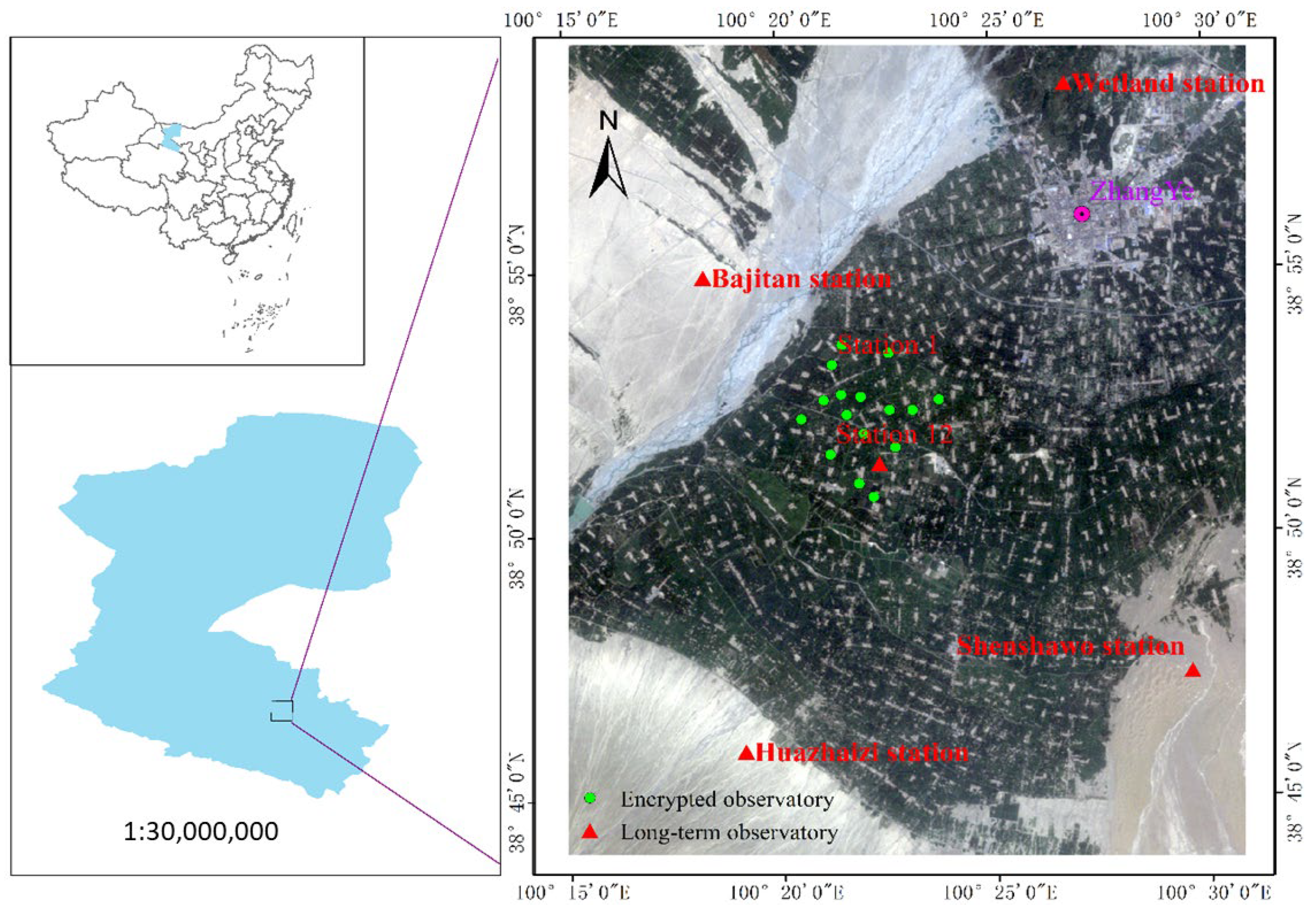
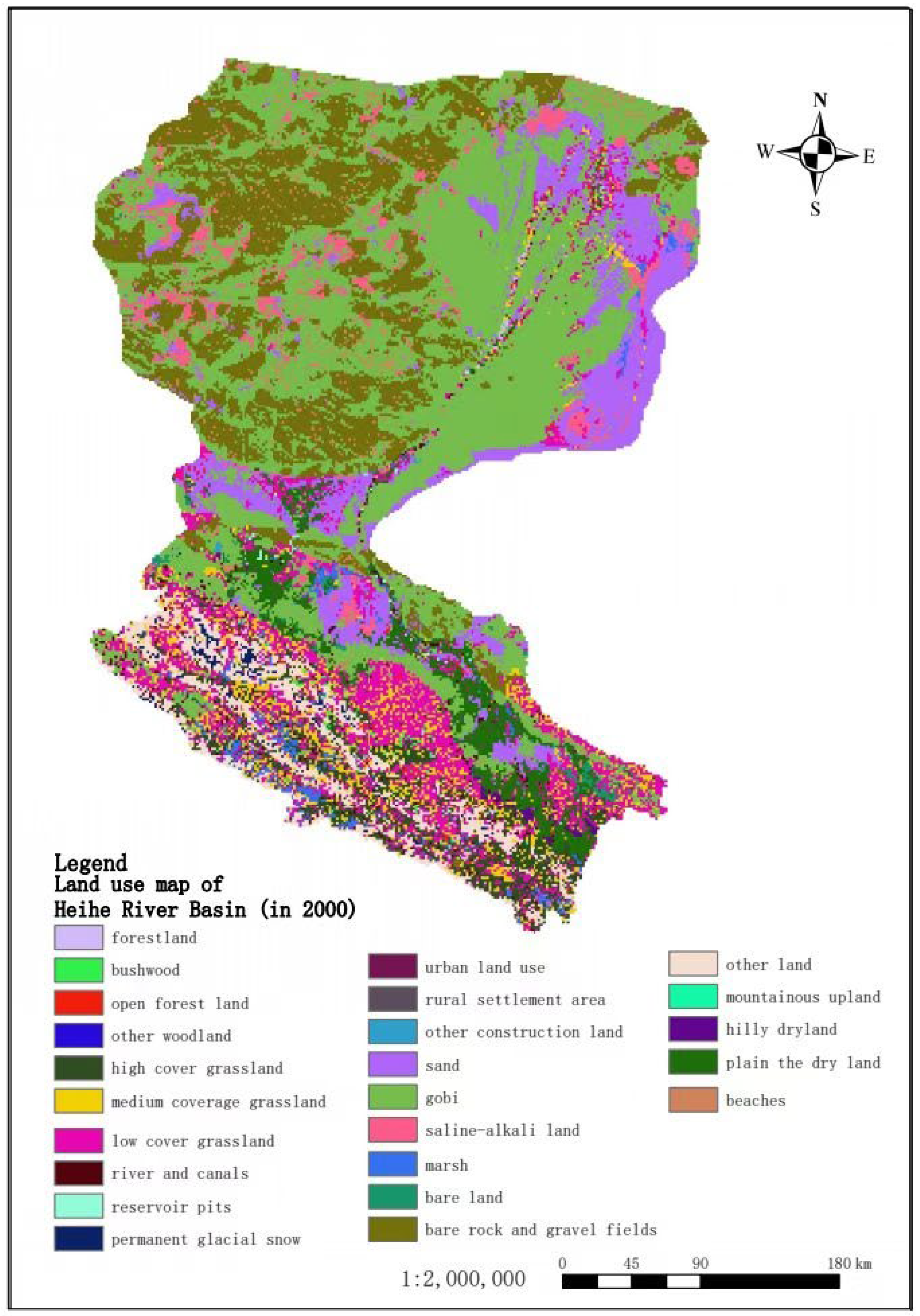
2.1. Research Area

The research area is located in Zhangye City, Gansu Province, which is the core oasis in the middle reaches of the Heihe River Basin (HRB) (100.104~100.853° E, 38.549~39.399° N). The climate type is semi-arid and arid in the middle temperate zone, with an average altitude of 1474 m. The annual average temperature is 7.3 °C, the monthly average maximum temperature is 29.3 °C (July), and the monthly average minimum temperature is −16.2 °C (January). The average annual precipitation is 130.44 mm, the average annual precipitation days are 51.6 days, and the average monthly precipitation days are 9.4 days (July). The area receives plenty of sunshine, evaporation is strong, the annual average evaporation is 2000~3500 mm, and the temperature difference between day and night is very large.
In this paper, six stations were selected. Daman superstation is located in the Daman irrigation district, Zhangye city, Gansu province. The underside of encryption station 1 is vegetable field, the underside of encryption station 12 is cornfield, and the Huazhaizi station is a typical desert subsurface with sparse red sand and pearl sand growing on the surface. In the Bajitan station, the surface is mainly coarse sand and gravel, the surface is short of water and plants are scarce, and only some drought-tolerant plants such as tamarisk and camel thorn grow. The Shenshawo station is a barren area mainly covered by sand with rare plants and dry air; in the Wetland station, the underlying surface is wetland with adequate moisture and dense vegetation. The information of these stations in this paper was collected from a large station in the Heihe Hydrological Remote Sensing Experiment, in which vegetable fields and cornfields are subsite stations of the Daman Super Station. These sites are complete and informative and suitable for research. The specific information and distribution of sites in the research area is shown in Table 1 and Figure 1. The land cover of the Heihe River Basin is shown in Figure 2 [24].

2.2. Instrument and Test Content

An imaging spectrometer, a light detection and ranging (lidar) system, a charge-coupled device (CCD), a multi-angle thermal infrared camera, and a microwave radiometer were used in the test. In the whole HRB, the ordinary automatic meteorological station (AMS) measures the radiation, precipitation, air pressure, wind speed and direction, air temperature, humidity, soil moisture and temperature profiles, and soil heat flux. The superstation was outfitted with an EC system, a Bowen ration energy balance system, an LAS (large aperture scintillometer), and a lysimeter (optional) to measure fluxes at multiple scales. In addition, the standard observations performed in an ordinary station, photosynthetically active radiation (PAR) and land surface temperature (LST) are measured at a superstation. Detailed instrument introduction can be found in Li’s article [25,26].

2.3. Research Data

The data needed in this paper are from the thematic test of evapotranspiration over non-uniform surface in the combined experiment of integrated remote sensing observation of ecohydrological processes in the Heihe River Basin (referred to as “Joint telemetry Experimental Study in the Heihe River Basin”, HiWATER [23,26,27]). Six stations were selected for this study, namely, Bajitan station, Huazhaizi station, Shenshawo station, wetland station in the middle reaches of the Heihe River (Gobi, desert, dune and wetland will be used in the following) and two encrypted stations 1 and 12 in the Daman irrigation area (vegetable field and cornfield will be used in the following). EC observation data of horizontal wind velocity, air temperature, water vapor density, carbon dioxide concentration and latent heat flux were selected and obtained from Heihe Plan Data Management Center Network (http://westdc.westgis.ac.cn accessed on: 1 September 2022). The data averaging interval was 30 min, among which the data before June 25 in wetland station and August 2 in Bajitan Station were missing. The start and end times of research area sites and data are shown in Table 1.

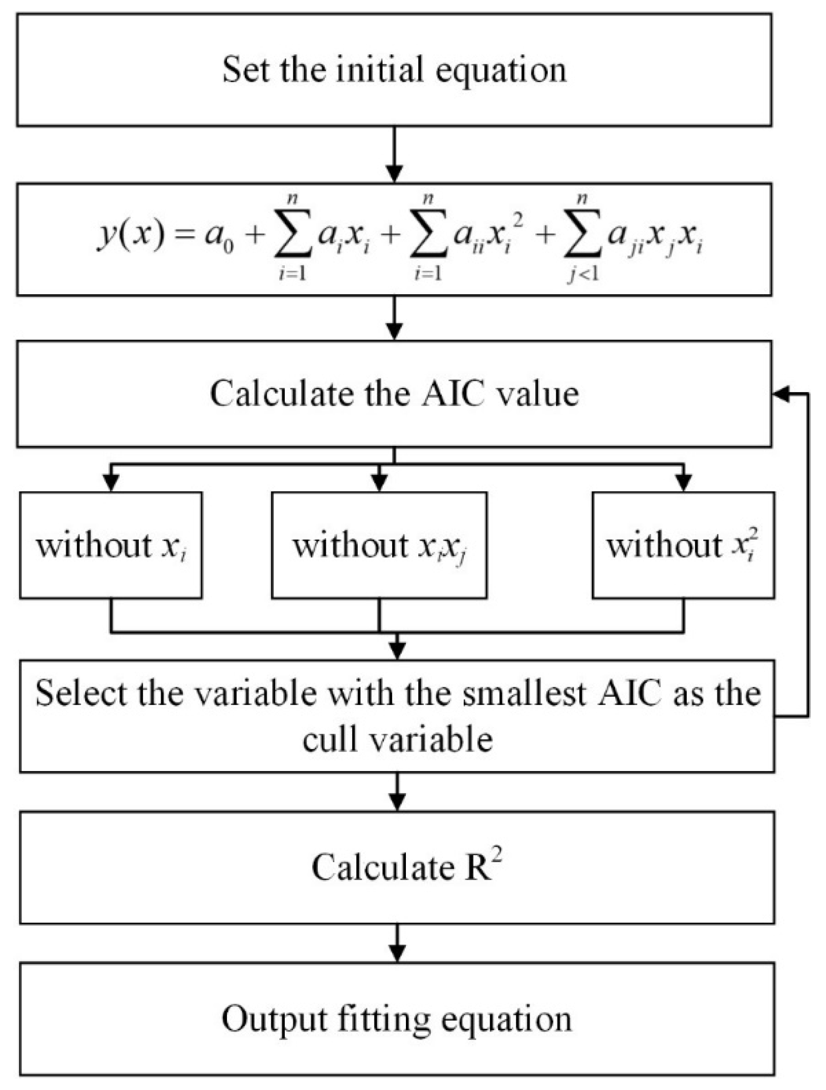
2.4. Data Processing

There are a small number of missing values in the EC observations. The interpolation data is mainly LE, and the missing part is mainly concentrated in the early and late time periods. The trend of LE in these two time periods is not obvious, and it has no influence on the analysis. Data is complemented by linear interpolation.
Stepwise regression analyses considered the contribution of independent variables and introduced screening results in descending order. Model identification only needs to optimize the coefficients of each input, and then uses AIC (Akaike information criterion) criterion to realize the automatic optimization of parameters, so it has been widely used [28].
In this paper, correlation coefficients (R) and stepwise regression methods need to be applied in the analysis of LE and its drivers. Related introductions are as follows:
The R has been widely used to measure the average discrepancy between models, though they are oversensitive to high extreme values (outliers) [29,30]. R is defined as:
R = 1 n i = 1 n ( Q 0 ( i ) Q 0 ¯ ) ( Q f ( i ) Q f ¯ ) 1 n i = 1 n ( Q 0 ( i ) Q 0 ) 2 1 n i = 1 n ( Q f ( i ) Q f ) 2
Akaike’s information criterion (AIC) is based on the information-theoretic approaches [31]. It is a standard for assessing the complexity of statistical models and measuring the goodness of statistical model fitting. When performing model training, the complexity of the model tends to increase with increased amount of data. At the same time, it is difficult to avoid over-fitting problems. In order to avoid over-fitting of the model, AIC and BIC (Bayesian Information Criterion) methods are often used. The penalty term of the BIC method is larger than the AIC method, so that in the case of a large sample size, a more desirable result is obtained [32]. When we use AIC to evaluate the model fit, we should give priority to models with the lowest AIC value to avoid over fitting [33].
In the general case, AIC can be expressed as:
A I C = 2 k 2 ln ( L )
where k is the number of parameters and L is the likelihood function.
The model’s error is subject to an independent normal distribution:
A I C = 2 k + n ln ( R S S / n )
where n is observation number and RSS (Residual Sum of Squares) is the sum of the residuals.
In view of the multiple impact factors often involved in multiple regression analysis, the computing cost can be very high to obtain the full set of parameters [34]. Using stepwise regression is a robust method [35]. The stepwise regression model in accordance with the quadratic response surface model is given as:
y ( x ) = a 0 + i = 1 n a i x i + i = 1 n a i i x i 2 + j < 1 n a j i x j x i
The stepwise regression method introduces the significant independent variables into the regression equation according to the order of the independent variables in the model. It re-examines the significance level test at the pre-specified F or AIC level and eliminates variables that are not significantly affected by the dependent variable, until the variables are not able to make the model better by reintroducing the independent variables, that is, completing the regression process and obtaining the optimal regression equation [34,35]. According to Equation (4), the objects of stepwise regression can be linear or nonlinear relations among factors, and the interaction between factors can be considered. Calculation flow chart is shown in Figure 3.

3. Results

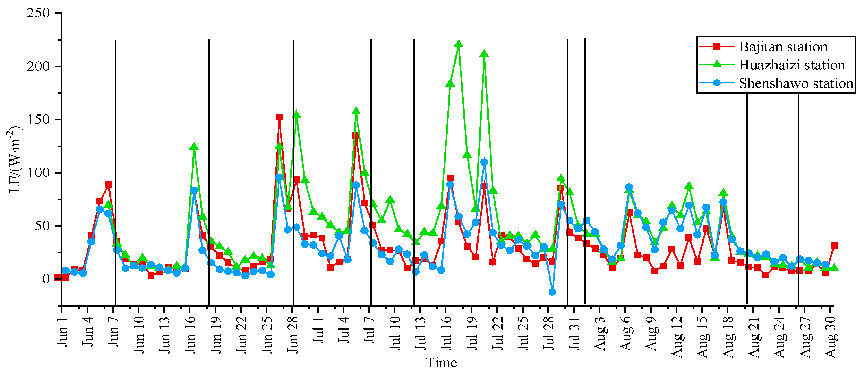
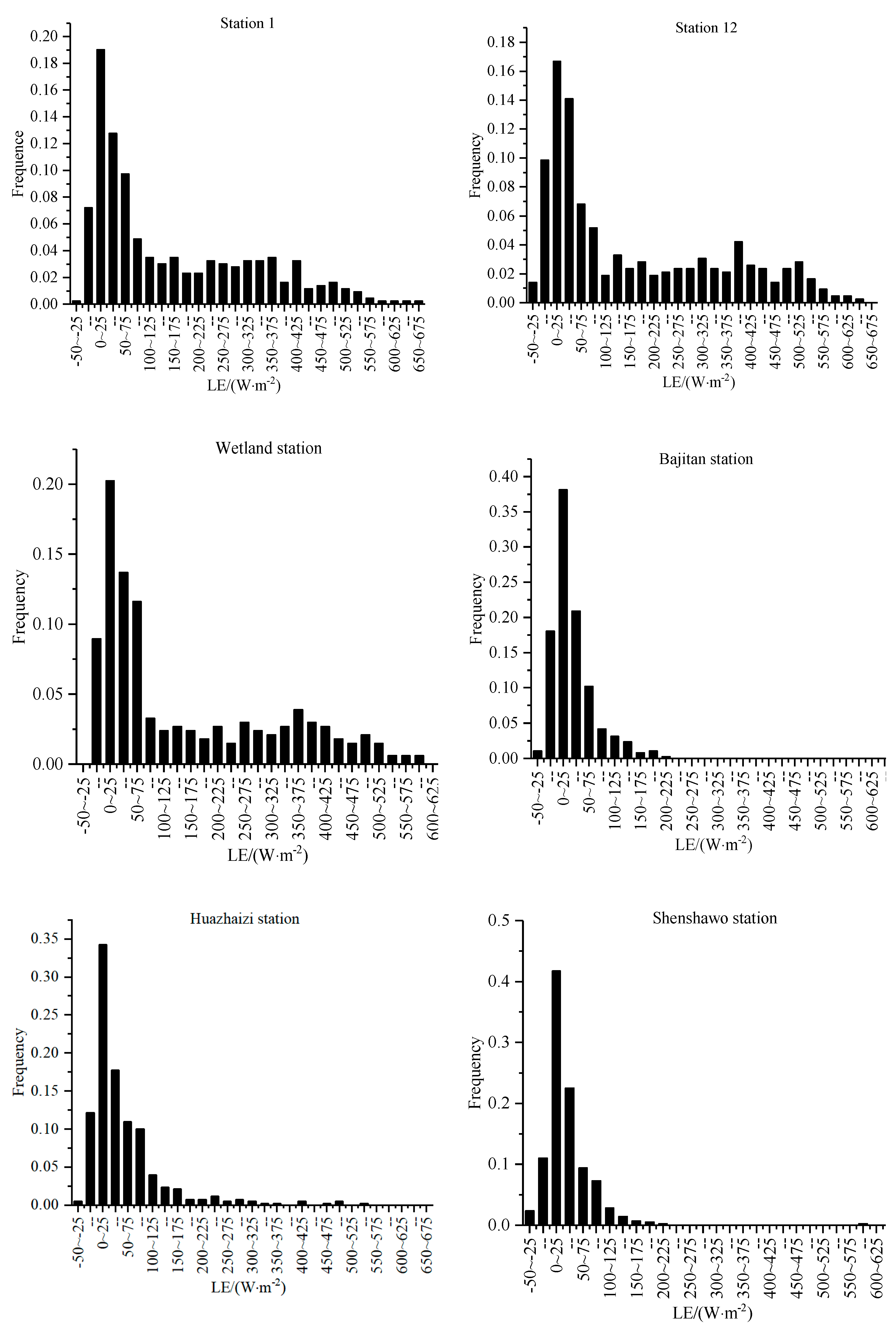
3.1. Analysis of LE Variation Trend under Different Underlying Surface Types

LE data of June, July and August 2012 are selected to draw LE time series diagram according to different underlying surface types. As can be seen from Figure 3, the current underlying surface conditions (soil moisture content and vegetation coverage) are similar, and LE has a similar trend over time; in combination with the historical weather in Zhangye city in June, July and August 2012, the fluctuation of LE trend line is further obtained, which is roughly consistent with the sunny and rainy changes in the weather. In this paper, with sunny days taken as a control variable, station data (vertical line marker) with weather conditions as sunny days within three months were selected to further analyze the characteristics and distribution rules of LE days.
Taking sunny days as a control condition and according to different sites, we selected 9-day LE data of 8 June, 19 June, 29 June, 9 July, 13 July, 31 July, 2 August, 21 August, and 27 August 2012, and respectively mapped the nine days of LE intraday frequency distribution histogram. LE days statistical results are also given. From Figure 4 and Table 2, it can be seen that the peak value and standard deviation of each site are significantly different, and the difference is closely related to the type of underlying surface. The peak value of LE was 661.3 W/m2 for vegetable land, and the minimum value was 201.2 W/m2 for dune. The maximum LE standard deviation is cornfield, with a value of 180.8 W/m2; the minimum is dune, with a value of 39.3 W/m2. The standard deviation can reflect the degree of dispersion of the research object, and the kurtosis can reflect the steepness and slowness of distribution pattern, that is, the distribution of LE value in vegetable field, cornfield and wetland is relatively discrete and slow, while that in Gobi, dune and desert is relatively concentrated and steep. At the same time, the cumulative values of Gobi, dune and desert on the −50~100 W/m2 interval are 92.4%, 89.5% and 94.1%, respectively, and the cumulative values of vegetable land, corn land and wetland on the −50~100 W/m2 interval are 53.8%, 54% and 57.7%, respectively, which can also reflect that the dispersion degree and standard deviation of diurnal distribution of LE are consistent.
Although the underlying surface conditions of each site are different, they can be roughly divided into two types by analyzing the above data comprehensively: dry (Gobi, dune, desert) and wet (vegetable, corn, and wetland). LE value of underlying surface is concentrated in the range of −50~100 W/m2 under the dry environment. Under the humid environment of the underlying surface, the LE value is also concentrated in −50~100 W/m2, but with a high degree of dispersion, 42.2~46.2% of LE value is distributed over 100 W/m2. Evapotranspiration requires three driving factors: energy supply, adequate vegetation water supply, high summer temperatures and surface temperature. At the same time, the water vapor flowing upward diffusion and evaporation quantity increase [36], relatively humid environment, vegetation coverage in the dry environment, lack of soil moisture, plant transpiration and soil evaporation lead to lack of corresponding water supply, and the evaporation quantity is very low [37]. Therefore, compared with the dry-land environment, the latent heat flux of wetland environment has a large change range, which can also be confirmed in the results of the study [38].

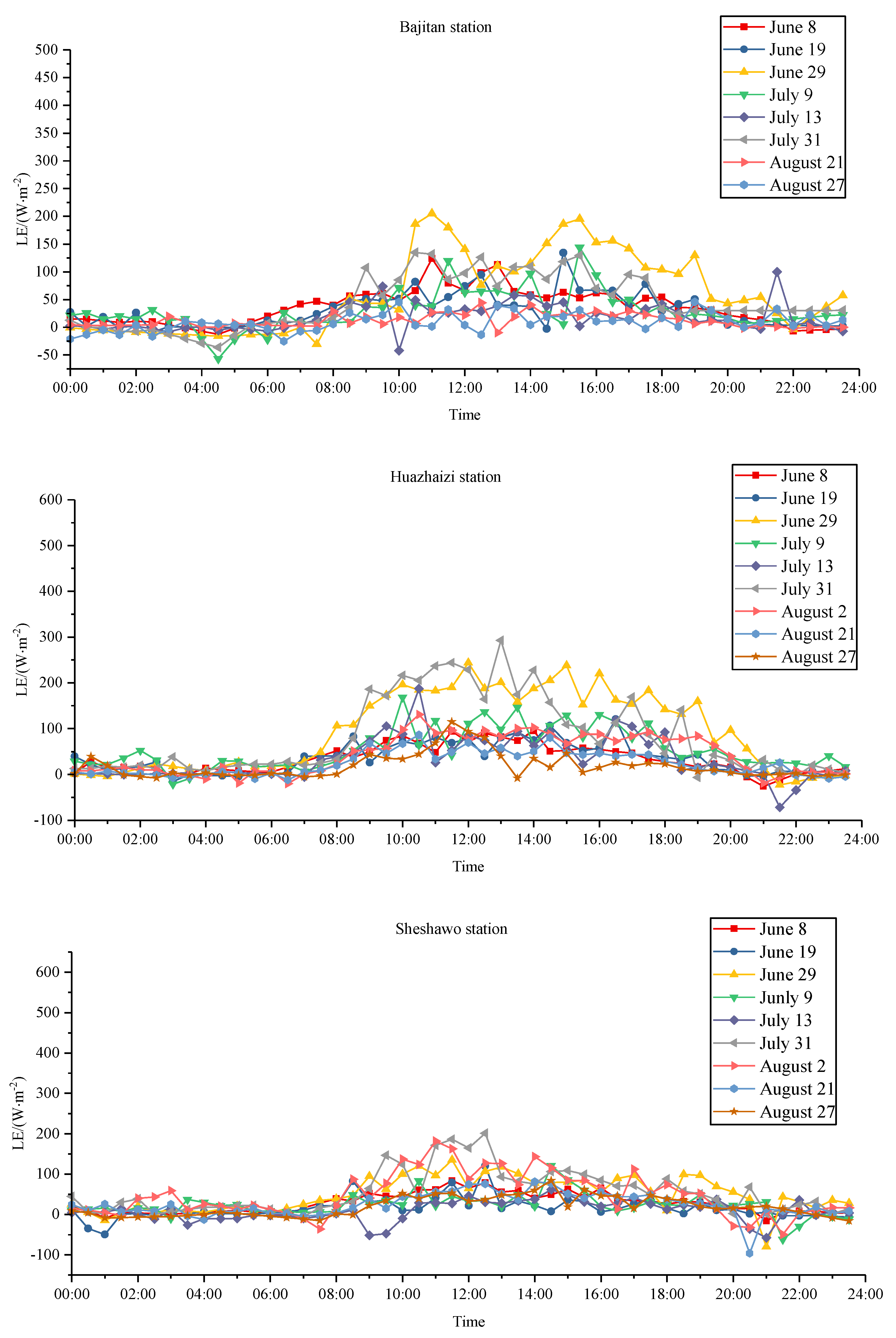
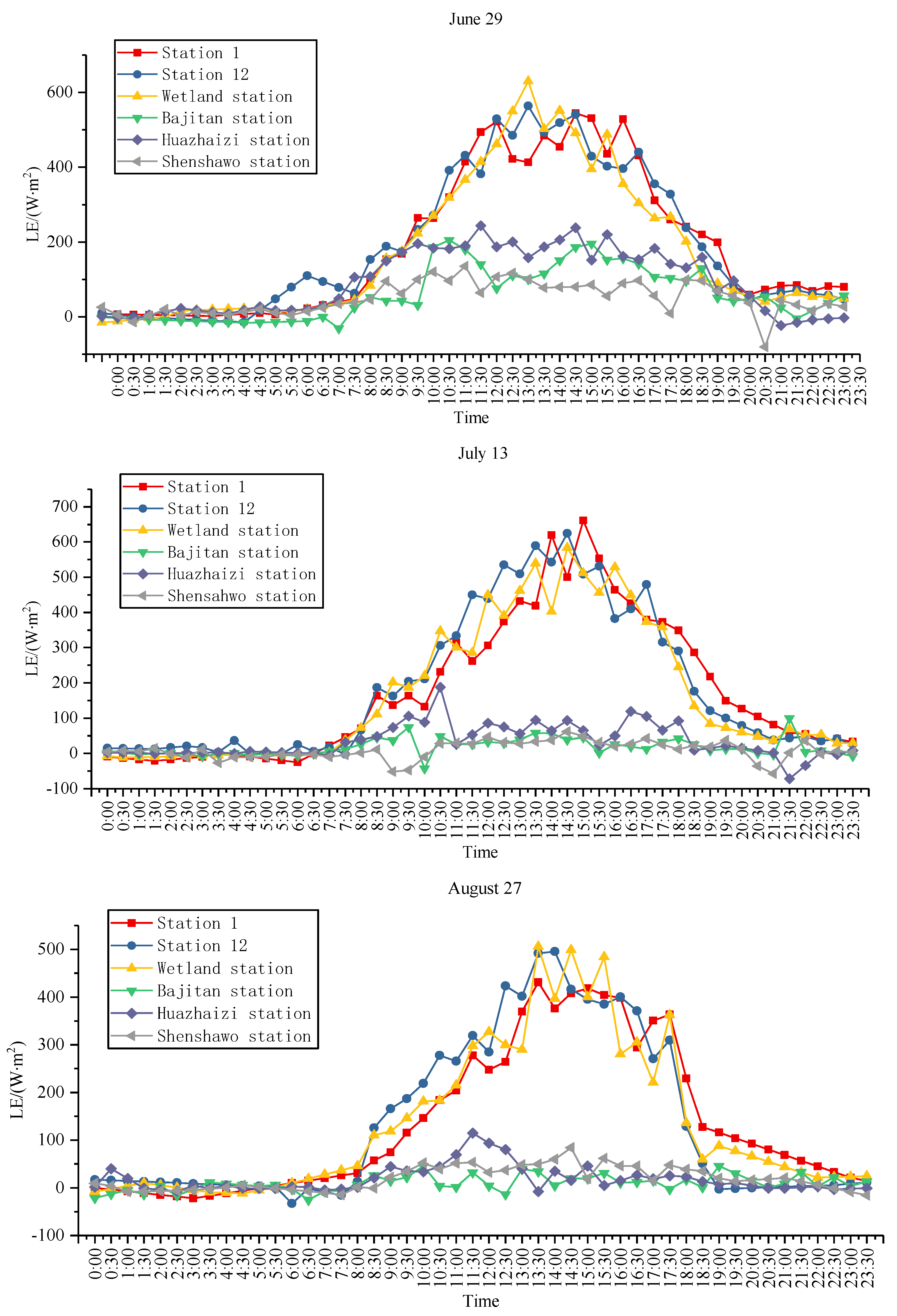
3.2. Analysis of Intraday Variation Trend of LE on Different Underlying Surfaces

For different sites, the variation trend of the same site within LE days at different times was analyzed. Figure 5 shows that the variation trend of different sites within LE days was mostly the same. According to the climatic conditions at different times in June, July and August, the lack of EC observation data is based on sunny days and less data loss. 29 June, 13 July, and 27 August were selected as typical days to further study the variation trend of LE intraday at different sites on the same time scale (see Figure 6 for details).
On 29 June, the LE intraday trend lines of all stations were significantly affected by the underlying surface. At 9:30, the LE intraday trend lines of all stations showed scattered changes. At this time, the LE intraday trend lines of vegetable fields, cornfields and wetlands continued to rise. At 12:00, vegetable and cornfields showed maximum value, and then the upward trend slowed down. The minimum value appeared at 12:30 and 13:00, respectively. From 12:00 to 15:00, the overall horizontal vibration of vegetable field and cornfield presented a multi-peak situation. The intraday trend line of wetland was slightly different from that of cornfield and wetland, reaching the maximum at 13:00, and then showing a tendency of oscillation and decline. Within LE days, the trend lines of Gobi, desert and dune were relatively flat. The internal trend line of the dune is the gentlest, with the lowest peak. There was no significant change throughout the day, and the desert was between the Gobi and the dune. The multi-peak trend of LE intraday trend line in vegetable and corn fields was mainly due to the obvious phenomenon of midday depression of crop, when vegetation stomata was closed and transpiration was weakened. From 15:00 to 16:00, solar radiation decreased, leaf water potential gradually rose, and vegetation transpiration recovered, which agrees with the law of evapotranspiration rate change previously reported in the literature [39].
On July 13, the patterns of LE intraday trend lines at each site were slightly different. The average value of LE in wetlands, vegetable fields and cornfields were at the highest level in three months, reaching the peak value within LE days from 14:00 to 15:00, and the peak form was a single peak. However, the average LE value of dune, desert and Gobi was at the lowest level in three months, and the trend line tends to be stable with little fluctuation. The daily average LE value was only 33.69 W/m2, 56.16 W/m2 and 34.83 W/m2.
The diurnal variation trend of LE at all stations on August 27 was basically consistent with that on July 13 [40]. The peak values of vegetable land, corn land and wetland decreased slightly from July to the lowest level in three months, among which the peak values of vegetable land decreased significantly [41].
After comprehensive analysis of the three days’ data, it is not difficult to find that there is little change in the daily LE trend line of each site on June 29, July 13, and August 27, but there is significant difference in the daily LE trend of different sites compared with the other sites.

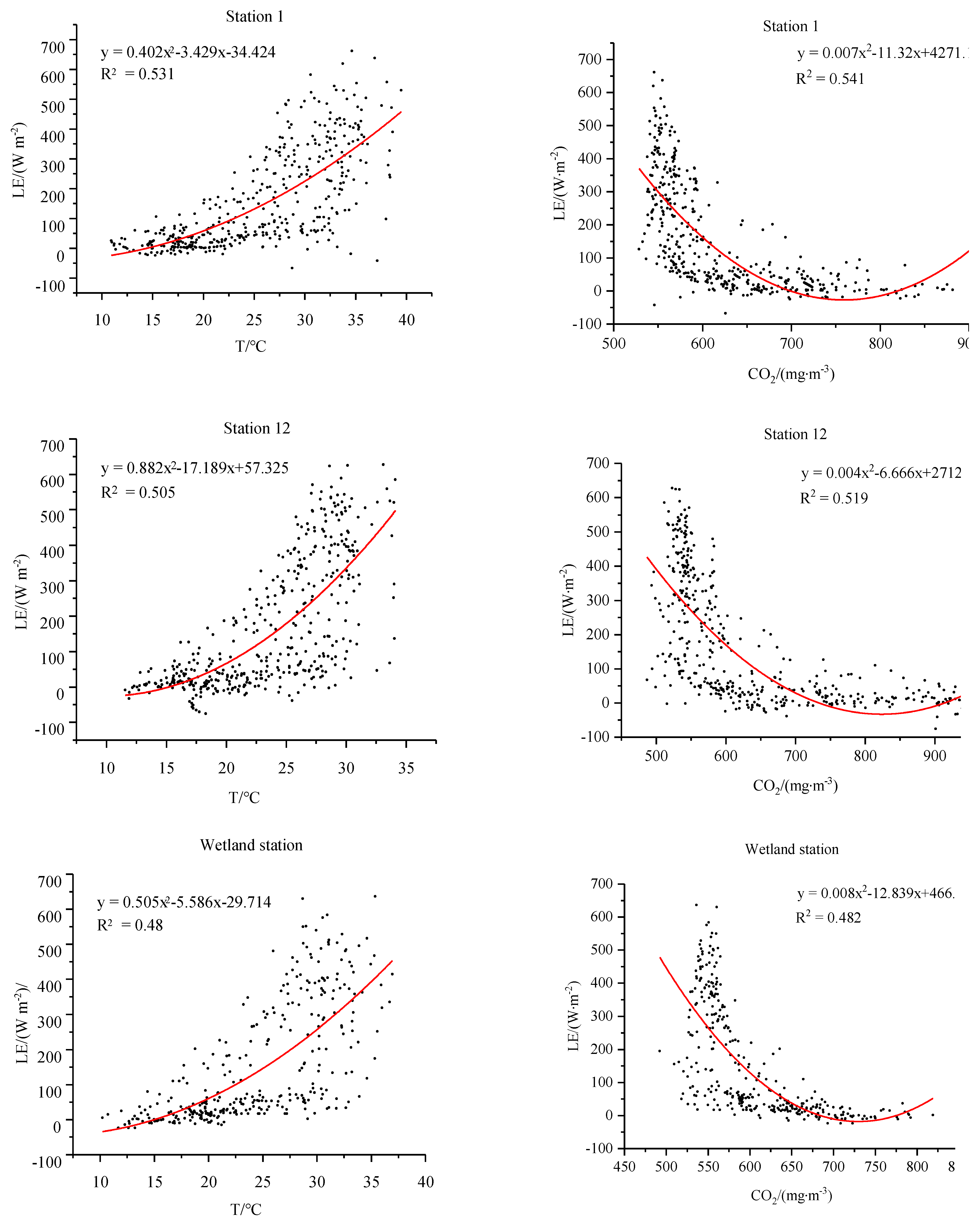
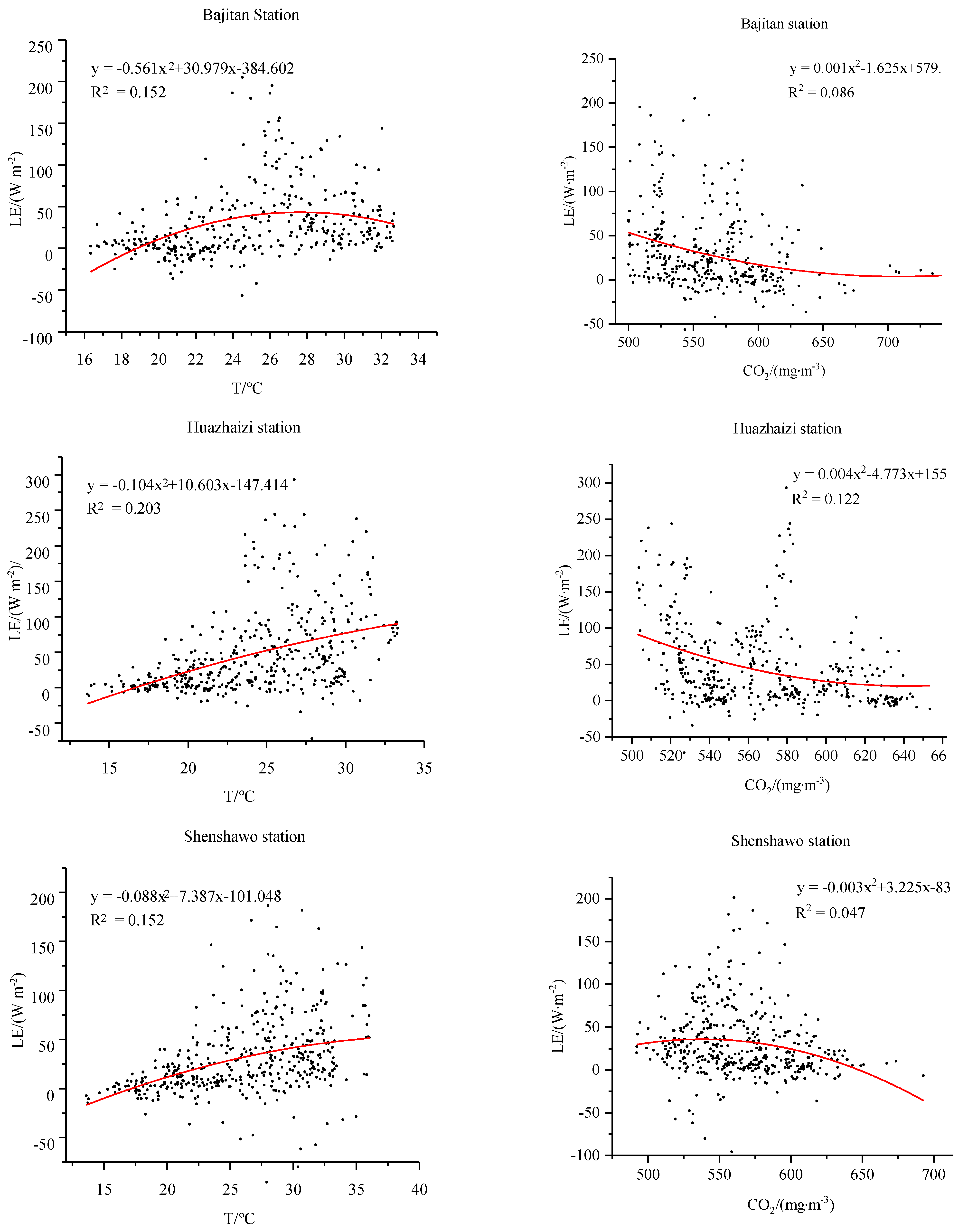
3.3. Analysis of LE Drivers for Different Underlying Surface Types

This part analyzes the correlation between LE and its driving factors under different underlying surface types. According to Table 3 and the correlation coefficient statistics of each driving factor, the LE of this site has a strong correlation with the two driving factors: temperature and CO2. According to the ranking of stations in Table 2, the correlation coefficients between temperature and LE were 0.72, 0.70, 0.31, 0.45, 0.39 and 0.68, respectively, and the correlation was extremely significant (p < 0.01). The correlation coefficients of CO2 and LE were 0.64, 0.64, 0.28, 0.34, 0.18, 0.65, respectively, and the correlation was very significant (p < 0.01). The correlation between water vapor density and LE was positive or negative, depending on the site. From the regression curve of Figure 7, it is concluded that in the case of abundant soil moisture, LE and temperature rise rapidly through exponential relationship, and the rising speed is significantly greater than when soil moisture is missing. LE and CO2 have similar trends with temperature [42]. It is noteworthy that the underlying surface of the sand dune is the Shenshawo station, and the increase of LE with CO2 does not immediately show a downward trend, but has a turning point, which is obviously different from the monotonous change of CO2 on the LE. In this paper, two drivers (air temperature and CO2) with high correlation at each site were further selected for stepwise regression analysis, and multiple regression equations were established, as shown in Table 4.
Figure 8 shows there is a positive correlation between air temperature and LE, because the altitude of Zhangye city is relatively high and the sunlight is sufficient, and the solar radiation will cause the temperature rise [43,44]. The opening and closing degree of plant stomata is closely related to the temperature, and the solar radiation provides an energy supply for the transpiration of plants, so LE increases with the temperature rise. There is a significant negative correlation between CO2 and LE, which is because the increase of CO2 concentration, the decrease of stomatal opening and stomatal conductance increases the resistance of water vapor transportation, leading to the decrease of transpiration and latent heat flux. The correlation between water vapor density and LE is positive or negative. It can be considered that under the type of underlying surface with high vegetation coverage of vegetable land, corn land and wetland, soil moisture content is high, and the size of surface LE is mainly contributed by plant transpiration. In Gobi, dune and desert, the influence of temperature and CO2 on LE is greatly reduced, and the correlation between water vapor density and LE changes from negative to positive. This is mainly because the underlying surface is composed of sand and gravel, and its particle size is large, and the contact area with air is also large relative to the soil, and the water is more likely to evaporate. At the same time, the specific heat capacity of sand is relatively small. This is mainly because the underlying surface is composed of sand and gravel. At the same time, due to the high temperature in summer, the soil water potential drops sharply, and the transpiration and respiration of plants are restricted. At this time, LE is mainly provided by soil evaporation. Currently, soil evaporation leads to LE as well. As can be seen from Table 4, the correlation and credibility of the model established by considering the dual factors of temperature and CO2 on LE have been improved, indicating that the influences of temperature and CO2 on LE are mutually complementary and affect each other through the transpiration and respiration of plants.

3.4. Deficiencies and Discussions

Based on the EC observation data of the HiWATER test, this study discussed and analyzed the characteristics of evapotranspiration and the impact of various drivers on LE fluxes under different underlying surface types. Studies have shown that different conditions of dry (dune, desert, Gobi) and wet (vegetable land, corn land, wetland) underlying surface, latent heat flux distribution and intradernal variation trend are different, and vegetation cover has a greater impact on latent heat flux. Due to the limited observation time of this experiment, the corresponding hydrological annual frequency is single, which may be affected by the uneven distribution of rainfall in the year. In densely vegetated areas, precipitation is often more abundant. Because the plant roots store water, soil moisture is retained, so soil/plant moisture content is not the main reason for limiting evapotranspiration. In sparsely vegetated areas, precipitation is relatively low After precipitation occurs, soil water is rapidly replenished, but at the same time it also rapidly evaporates, soil water is difficult to retain, and soil/plant water content will limit the generation of evapotranspiration [45]. Therefore, in this study, it was found that in arid regions, evapotranspiration has no obvious correlation with each influencing factor, and the regularity of the corresponding data is even worse, so the evapotranspiration model estimation featuring vegetation cover has more potential [46,47,48]. Through the analysis of climate, environment and geomorphology, the conclusions obtained are more referential, which can provide a reliable reference for the study of drivers affecting farmland irrigation, drainage and evapotranspiration [49].
The drivers of latent heat flux under different underlying surface types are various, as well as the degree of correlation. There is not a simple linear relationship between the drivers and latent heat flux, and there is a turning point in the influence of CO2 on latent heat flux under dry conditions. The weather on the research day selected in this paper was sunny. The diurnal variation of ET is prone to obvious mutation within a certain time after the occurrence of precipitation. However, due to the great influence of rainfall on EC observation instrument [50], the variation trend of latent heat flux under different weather conditions of sunny and rainy months in June, July and August in summer was not studied [27,51]. In addition, studies on latent heat flux and other meteorological factors have not been introduced [52].

4. Conclusions

Different underlying surface types will affect the distribution characteristics of latent heat flux, and the difference of latent heat flux is small under the condition of small difference in surface vegetation coverage and soil moisture.
In the same season, the diurnal variation trend of latent heat flux under the same underlying surface type was not significantly different, but the diurnal variation trend of LE under different underlying surface types was significantly different. When soil moisture is sufficient, latent heat flux will be affected by the midday depression of crop, and the change range is large. When soil moisture is deficient, latent heat flux fluctuates gently.
When the soil water supply is sufficient, the correlation between temperature and CO2 and latent heat flux is strong. As air temperature rises, soil evaporation and plant transpiration strengthen, and latent heat flux increases; CO2 concentration affects stomatal resistance, so that latent heat flux decreases with increasing CO2 concentration; when soil water supply is sufficient, the synergistic effect of temperature and CO2 has a great impact on latent heat flux through transpiration and respiration of plants.
This paper only compared and analyzed the relationship between influence factors and latent heat flux of all stations in the middle reaches of the Heihe River in June, July, and August 2012, which was limited in terms of time scale. Therefore, more studies are needed to reveal the role and influence of evapotranspiration in surface energy transmission and water circulation.

Author Contributions

J.H. and Q.-M.L. were responsible for the original concept and writing the paper. W.-C.W. and Y.-R.W. processed the data and conducted the program design. D.-M.X. revised the manuscript and shared numerous comments and suggestions to improve the study quality. All authors have read and agreed to the published version of the manuscript.

Funding

The authors are grateful to acknowledge the funding support from the Project of Key Science and Technology of the Henan Province (No: 202102310259; No: 202102310588), Henan Province University scientific and technological innovation team (No: 18IRTSTHN009).

Data Availability Statement

Not applicable.

Conflicts of Interest

The authors declare that they have no conflict of interest.

References

  1. Chau, K. Use of Meta-Heuristic Techniques in Rainfall-Runoff Modelling. Water 2017, 9, 186. [Google Scholar] [CrossRef] [Green Version]
  2. Zhang, Z.; Qin, H.; Yao, L.; Liu, Y.; Jiang, Z.; Feng, Z.; Ouyang, S. Improved Multi-objective Moth-flame Optimization Algorithm based on R-domination for cascade reservoirs operation. J. Hydrol. 2020, 581, 124431. [Google Scholar] [CrossRef]
  3. Feng, F.; Li, X.; Yao, Y.; Liang, S.; Chen, J.; Zhao, X.; Jia, K.; Pintér, K.; McCaughey, J.H. An empirical orthogonal function-based algorithm for estimating terrestrial latent heat flux from eddy covariance, meteorological and satellite observations. PLoS ONE 2016, 11, e0160150. [Google Scholar] [CrossRef] [PubMed]
  4. Wang, K.; Dickinson, R.E. A review of global terrestrial evapotranspiration: Observation, modeling, climatology, and climatic variability. Rev. Geophys. 2012, 50, RG2005. [Google Scholar] [CrossRef]
  5. Wang, M.; Zhang, Y.; Lu, Y.; Gong, X.; Gao, L. Detection and attribution of reference evapotranspiration change (1951–2020) in the upper Yangtze River Basin of China. J. Water Clim. Chang. 2021, 12, 2624–2638. [Google Scholar] [CrossRef]
  6. Priestley, C.H.B.; Taylor, R.J. On the Assessment of Surface Heat Flux and Evaporation Using Large-Scale Parameters. Mon. Weather. Rev. 1972, 100, 81–92. [Google Scholar] [CrossRef]
  7. Talsma, C.J.; Good, S.P.; Jimenez, C.; Martens, B.; Fisher, J.B.; Miralles, D.G.; McCabe, M.F.; Purdy, A.J. Partitioning of evapotranspiration in remote sensing-based models. Agric. For. Meteorol. 2018, 260–261, 131–143. [Google Scholar] [CrossRef]
  8. Yin, Y.; Wu, S.; Chen, G.; Dai, E. Attribution analyses of potential evapotranspiration changes in China since the 1960s. Theor. Appl. Climatol. 2010, 101, 19–28. [Google Scholar] [CrossRef]
  9. Moazenzadeh, R.; Mohammadi, B.; Shahaboddin, S.; Chau, K.-W. Coupling a firefly algorithm with support vector regression to predict evaporation in northern Iran. Eng. Appl. Comput. Fluid Mech. 2018, 12, 584–597. [Google Scholar] [CrossRef] [Green Version]
  10. Wang, Z.; Ye, A.; Wang, L.; Liu, K.; Cheng, L. Spatial and temporal characteristics of reference evapotranspiration and its climatic driving factors over China from 1979–2015. Agric. Water Manag. 2019, 213, 1096–1108. [Google Scholar] [CrossRef]
  11. Zhang, R.; Xu, X.; Liu, M.; Zhang, Y.; Xu, C.; Yi, R.; Luo, W. Comparing evapotranspiration characteristics and environmental controls for three agroforestry ecosystems in a subtropical humid karst area. J. Hydrol. 2018, 563, 1042–1050. [Google Scholar] [CrossRef]
  12. Zhang, Y.; Kang, S.; Ward, E.J.; Ding, R.; Zhang, X.; Zheng, R. Evapotranspiration components determined by sap flow and microlysimetry techniques of a vineyard in northwest China: Dynamics and influential factors. Agric. Water Manag. 2011, 98, 1207–1214. [Google Scholar] [CrossRef]
  13. Barraza Bernadas, V.; Grings, F.; Restrepo-Coupe, N.; Huete, A. Comparison of the performance of latent heat flux products over southern hemisphere forest ecosystems: Estimating latent heat flux error structure using in situ measurements and the triple collocation method. Int. J. Remote Sens. 2018, 39, 6300–6315. [Google Scholar] [CrossRef]
  14. Barraza, V.; Grings, F.; Franco, M.; Douna, V.; Entekhabi, D.; Restrepo-Coupe, N.; Huete, A.; Gassmann, M.; Roitberg, E. Estimation of latent heat flux using satellite land surface temperature and a variational data assimilation scheme over a eucalypt forest savanna in Northern Australia. Agric. For. Meteorol. 2019, 268, 341–353. [Google Scholar] [CrossRef]
  15. Eswar, R.; Sekhar, M.; Bhattacharya, B.K. Comparison of three remote sensing based models for the estimation of latent heat flux over India. Hydrol. Sci. J.-J. Des. Sci. Hydrol. 2017, 62, 2705–2719. [Google Scholar] [CrossRef]
  16. Evett, S.R.; Schwartz, R.C.; Howell, T.A.; Baumhardt, R.L.; Copeland, K.S. Can weighing lysimeter ET represent surrounding field ET well enough to test flux station measurements of daily and sub-daily ET. Adv. Water Resour. 2012, 50, 79–90. [Google Scholar] [CrossRef]
  17. Maltese, A.; Awada, H.; Capodici, F.; Ciraolo, G.; La Loggia, G.; Rallo, G. On the Use of the Eddy Covariance Latent Heat Flux and Sap Flow Transpiration for the Validation of a Surface Energy Balance Model. Remote Sens. 2018, 10, 195. [Google Scholar] [CrossRef] [Green Version]
  18. Swinbank, W.C. The measurement of vertical transfer of heat and water vapor by eddies in the lower atmosphere. J. Meteorol. 1951, 8, 135–145. [Google Scholar] [CrossRef]
  19. Todd, R.W.; Evett, S.R.; Howell, T.A. The Bowen ratio-energy balance method for estimating latent heat flux of irrigated alfalfa evaluated in a semi-arid, advective environment. Agric. For. Meteorol. 2000, 103, 335–348. [Google Scholar] [CrossRef]
  20. Wang, X.; Wang, C.; Bond-Lamberty, B. Quantifying and reducing the differences in forest CO2-fluxes estimated by eddy covariance, biometric and chamber methods: A global synthesis. Agric. For. Meteorol. 2017, 247, 93–103. [Google Scholar] [CrossRef]
  21. Ghorbani, M.A.; Kazempour, R.; Chau, K.-W.; Shamshirband, S.; Ghazvinei, P.T. Forecasting pan evaporation with an integrated artificial neural network quantum-behaved particle swarm optimization model: A case study in Talesh, Northern Iran. Eng. Appl. Comput. Fluid Mech. 2018, 12, 724–737. [Google Scholar] [CrossRef]
  22. Wilson, K.B.; Hanson, P.J.; Mulholland, P.J.; Baldocchi, D.D.; Wullschleger, S.D. A comparison of methods for determining forest evapotranspiration and its components: Sap-flow, soil water budget, eddy covariance and catchment water balance. Agric. For. Meteorol. 2001, 106, 153–168. [Google Scholar] [CrossRef]
  23. Li, X.; Liu, S.; Ma, M.; Xiao, Q.; Liu, Q.; Jin, R.; Che, T.; Wang, W.; Qi, Y. HiWATER: An Integrated Remote Sensing Experiment on Hydrological and Ecological Processes in the Heihe River Basin. Adv. Earth Sci. 2012, 27, 481–498. [Google Scholar] [CrossRef]
  24. Wang, J.; Zhao, J.; Wang, X. Landscape types of the Heihe River Basin (2000). Natl. Tibet. Plateau Data Center 2013. [Google Scholar] [CrossRef]
  25. Liu, S.M.; Xu, Z.W.; Wang, W.Z.; Jia, Z.Z.; Zhu, M.J.; Bai, J.; Wang, J.M. A comparison of eddy-covariance and large aperture scintillometer measurements with respect to the energy balance closure problem. Hydrol. Earth Syst. Sci. 2011, 15, 1291–1306. [Google Scholar] [CrossRef] [Green Version]
  26. Li, X.; Cheng, G.; Liu, S.; Xiao, Q.; Ma, M.; Jin, R.; Che, T.; Liu, Q.; Wang, W.; Qi, Y.; et al. Heihe Watershed Allied Telemetry Experimental Research (HiWATER): Scientific Objectives and Experimental Design. Bull. Am. Meteorol. Soc. 2013, 94, 1145–1160. [Google Scholar] [CrossRef]
  27. Yu, L.-P.; Huang, G.-H.; Liu, H.-J.; Wang, X.-P.; Wang, M.-Q. Experimental Investigation of Soil Evaporation and Evapotranspiration of Winter Wheat under Sprinkler Irrigation. Agric. Sci. China 2009, 8, 1360–1368. [Google Scholar] [CrossRef]
  28. Wu, C.L.; Chau, K.W. Rainfall–runoff modeling using artificial neural network coupled with singular spectrum analysis. J. Hydrol. 2011, 399, 394–409. [Google Scholar] [CrossRef] [Green Version]
  29. Legates, D.R.; McCabe, G.J., Jr. Evaluating the use of “goodness-of-fit” measures in hydrologic and hydroclimatic model validation. Water Resour. Res. 1999, 35, 233–241. [Google Scholar] [CrossRef]
  30. Wang, W.-C.; Chau, K.-W.; Cheng, C.-T.; Qiu, L. A comparison of performance of several artificial intelligence methods for forecasting monthly discharge time series. J. Hydrol. 2009, 374, 294–306. [Google Scholar] [CrossRef]
  31. Shibata, R. Selection of the order of an autoregressive model by Akaike’s information criterion. Biometrika 1976, 63, 117–126. [Google Scholar] [CrossRef]
  32. Yafune, A.; Narukawa, M.; Ishiguro, M. A Note on Sample Size Determination for Akaike Information Criterion (AIC) Approach to Clinical Data Analysis. Commun. Stat. Theory Methods 2005, 34, 2331–2343. [Google Scholar] [CrossRef]
  33. Arnold, T.W. Uninformative Parameters and Model Selection Using Akaike’s Information Criterion. J. Wildl. Manag. 2010, 74, 1175–1178. [Google Scholar] [CrossRef]
  34. Liao, X.; Li, Q.; Yang, X.; Zhang, W.; Li, W. Multiobjective optimization for crash safety design of vehicles using stepwise regression model. Struct. Multidiscip. Optim. 2008, 35, 561–569. [Google Scholar] [CrossRef]
  35. Krishnaiah, P.R. 37 Selection of variables under univariate regression models. In Handbook of Statistics; Elsevier: Amsterdam, The Netherlands, 1982; Volume 2, pp. 805–820. [Google Scholar]
  36. Liu, S.; Li, X.; Xu, Z.; Che, T.; Xiao, Q.; Ma, M.; Liu, Q.; Jin, R.; Guo, J.; Wang, L.; et al. The Heihe Integrated Observatory Network: A Basin-Scale Land Surface Processes Observatory in China. Vadose Zone J. 2018, 17, 180072. [Google Scholar] [CrossRef]
  37. Zhang, D.; Liu, X.; Zhang, Q.; Liang, K.; Liu, C. Investigation of factors affecting intra-annual variability of evapotranspiration and streamflow under different climate conditions. J. Hydrol. 2016, 543, 759–769. [Google Scholar] [CrossRef]
  38. Harmel, R.D.; Patricia, K. Smith. Consideration of measurement uncertainty in the evaluation of goodness-of-fit in hydrologic and water quality modeling. J. Hydrol. 2007, 337, 326–336. [Google Scholar] [CrossRef]
  39. Reddy, K.S.; Maruthi, V.; Pankaj, P.K.; Kumar, M.; Pushpanjali; Prabhakar, M.; Reddy, A.G.K.; Reddy, K.S.; Singh, V.K.; Koradia, A.K. Water Footprint Assessment of Rainfed Crops with Critical Irrigation under Different Climate Change Scenarios in SAT Regions. Water 2022, 14, 1206. [Google Scholar] [CrossRef]
  40. Dinpashoh, Y.; Jhajharia, D.; Fakheri-Fard, A.; Singh, V.P.; Kahya, E. Trends in reference crop evapotranspiration over Iran. J. Hydrol. 2011, 399, 422–433. [Google Scholar] [CrossRef]
  41. Chaouche, K.; Neppel, L.; Dieulin, C.; Pujol, N.; Ladouche, B.; Martin, E.; Salas, D.; Caballero, Y. Analyses of precipitation, temperature and evapotranspiration in a French Mediterranean region in the context of climate change. Comptes Rendus Geosci. 2010, 342, 234–243. [Google Scholar] [CrossRef]
  42. Chen, Y.; Xue, Y.; Hu, Y. How multiple factors control evapotranspiration in North America evergreen needleleaf forests. Sci. Total Environ. 2018, 622–623, 1217–1224. [Google Scholar] [CrossRef] [PubMed]
  43. Wang, K.; Wang, P.; Li, Z.; Cribb, M.; Sparrow, M. A simple method to estimate actual evapotranspiration from a combination of net radiation, vegetation index, and temperature. J. Geophys. Res. Atmos. 2007, 112. [Google Scholar] [CrossRef]
  44. Zhang, K.; Wang, R.Y.; Li, Q.Z.; Wang, H.L.; Zhao, H.; Yang, F.L.; Zhao, F.N.; Qi, Y. Effects of elevated CO2 concentration on production and water use efficiency of spring wheat in semi-arid area. Ying Yong Sheng Tai Xue Bao 2018, 29, 2959–2969. [Google Scholar] [CrossRef] [PubMed]
  45. Zhang, Y.; Wang, J.; Gong, S.; Xu, D.; Sui, J.; Wu, Z.; Mo, Y. Effects of film mulching on evapotranspiration, yield and water use efficiency of a maize field with drip irrigation in Northeastern China. Agric. Water Manag. 2018, 205, 90–99. [Google Scholar] [CrossRef]
  46. Hu, X.; Lei, H. Evapotranspiration partitioning and its interannual variability over a winter wheat-summer maize rotation system in the North China Plain. Agric. For. Meteorol. 2021, 310, 108635. [Google Scholar] [CrossRef]
  47. Liu, Y.; Luo, Y. A consolidated evaluation of the FAO-56 dual crop coefficient approach using the lysimeter data in the North China Plain. Agric. Water Manag. 2010, 97, 31–40. [Google Scholar] [CrossRef]
  48. Zhao, N.; Liu, Y.; Cai, J.; Paredes, P.; Rosa, R.D.; Pereira, L.S. Dual crop coefficient modelling applied to the winter wheat–summer maize crop sequence in North China Plain: Basal crop coefficients and soil evaporation component. Agric. Water Manag. 2013, 117, 93–105. [Google Scholar] [CrossRef]
  49. Shahrokhnia, M.H.; Sepaskhah, A.R. Single and dual crop coefficients and crop evapotranspiration for wheat and maize in a semi-arid region. Theor. Appl. Climatol. 2013, 114, 495–510. [Google Scholar] [CrossRef]
  50. Ding, R.; Kang, S.; Li, F.; Zhang, Y.; Tong, L.; Sun, Q. Evaluating eddy covariance method by large-scale weighing lysimeter in a maize field of northwest China. Agric. Water Manag. 2010, 98, 87–95. [Google Scholar] [CrossRef]
  51. Afzal, M.; Ragab, R. Assessment of the potential impacts of climate change on the hydrology at catchment scale: Modelling approach including prediction of future drought events using drought indices. Appl. Water Sci. 2020, 10, 215. [Google Scholar] [CrossRef]
  52. Zhang, Y.-K.; Schilling, K. Effects of land cover on water table, soil moisture, evapotranspiration, and groundwater recharge: A field observation and analysis. J. Hydrol. 2006, 319, 328–338. [Google Scholar] [CrossRef]
Figure 1. Geographical location and site distribution map of the research area.
Water 14 03514 g001
Figure 2. Land cover map of the Heihe River Basin.
Water 14 03514 g002
Figure 3. Stepwise regression calculation flow chart.
Water 14 03514 g003
Figure 4. Frequency distribution within LE days under different underlying surface types.
Water 14 03514 g004
Figure 5. Histogram of LE frequency distribution for 9 days under different underlying surface types.
Water 14 03514 g005
Figure 6. LE intraday variation trend of nine days under different underlying surface types.
Water 14 03514 g006aWater 14 03514 g006b
Figure 7. LE intraday variation trend under different pad types on June 29, July 13 and August 27.
Water 14 03514 g007
Figure 8. Regression analysis curves of LE and influencing factors under different underlying surface types.
Water 14 03514 g008aWater 14 03514 g008b
Table 1. Site name and related information of the research area.
Site NameType of Underlay SurfaceAltitude (m)Data Start and End Time
station 1Vegetable ground1552.85 June–31 August
station 12Cornfield1559.31 June–31 August 31
Shenshawo stationDune1562.61 June–31 August (data unavailable on August 2)
Bajitan stationGobi1731.07 June–31 August
Huazhaizi stationDesert1549.42 June–30 August
Wetland stationWetland1460.026 June to 30 August
Table 2. LE statistical results of 9 days were synthesized under different types of underlying surfaces.
Site NameStandard Deviation
/(W/m2)
Average /(W/m2)Maximum
/(W/m2)
Minimum
/(W/m2)
KurtosisPartial
Degrees
station 1162.35154.12661.32−67.13−0.280.91
station 12180.83164.91627.27−75.64−0.690.23
Bajitan station40.9829.6205.03−56.52.991.6
Huazhaizi station56.4546.26292.91−71.792.341.55
Shenshawo
station
39.2829.90201.23−95.752.681.11
Wetland station168.83152.44636.53−23.52−0.40.13
Table 3. The correlation coefficients of LE and influencing factors under different underlying surface types.
Impact FactorWind Speed
/(m/s)
Temperature
/°C
Water Vapor Density/(g/m3)Carbon Dioxide/(mg/m3)
Site Name
station 10.38 **0.72 **−0.12−0.64 **
station 120.38 **0.70 **−0.13 **−0.64 **
Bajitan station0.20 **0.31 **0.16 **−0.28 **
Huazhaizi station0.22 **0.45 **0.10 *−0.34 **
Shenshawo station0.080.39 **0.180.18 **
Wetland station0.13 *0.68 **−0.14 **−0.65 **
Note: ** and * passed the significance test of 0.05 and 0.1 respectively.
Table 4. The multiple regression analysis of temperature and CO2 on LE under different underlying surface types.
Site NameStation 1Station 12Wetland Station
Fitting coefficientIntercept item519.66−58.56245.80 **
T49.57 **51.96 **--
CO2−2.39−0.830.002 **
T&CO2−0.07 **−0.07 **--
(CO2)20.002 **0.001 *0.004 **
(T)2----0.20 **
R20.590.560.51
Note: * indicates that the relationship is significant at the level of 0.1 by t-test. ** indicates that the relationship is significant at the level of 0.05 by t-test. T & CO2 represents the interaction between temperature and CO2. -- denotes that the data is empty.
Publisher’s Note: MDPI stays neutral with regard to jurisdictional claims in published maps and institutional affiliations.

