Modeling of Water Quality in West Ukrainian Rivers Based on Fluctuating Asymmetry of the Fish Population

Abstract

Increased concentrations of chemicals in surface waters affect the development of fish and the state of water bodies in general. In turn, the human consumption of fish that have accumulated heavy metals can cause toxicological hazards and endanger health. The importance of this area and the lack of water quality assessment methods in Ukraine based on the fluctuating asymmetry level of fish and the chemical parameters of water informed the object and aim of the current research. The object of this study was the use of fish populations as a bioindicator of water quality. The study had three purposes: (1) the determination of the dominant fish species and a comparison of their fluctuating asymmetry in the studied rivers; (2) the evaluation of the sensitivity/tolerance of the selected fish populations for assessing water quality; and (3) the creation of a model for assessing the water quality of the studied rivers based on the determined fluctuating asymmetry of the typical fish populations. Each of the studied fish populations had different frequency of fluctuating asymmetry (FFA) levels: the common roach had the highest value, and the silver crucian carp had the lowest. The final stage of the study was building an artificial neural network (ANN) model for predicting water quality based on the FFA of meristic features. Optimal results were obtained for the ANN model with the ReLU activation function and SGD optimization algorithm (MAPE = 6.7%; R² = 0.97187). Such values for the MAPE and R² indicators demonstrated that the level of agreement between the target and forecast data was satisfactory. The novelty of this research lay in the development of a model for assessing water quality based on the comparison of the fluctuating asymmetry values of the typical fish populations in the studied rivers.

1. Introduction

The environmental assessment of surface waters in Ukraine, as in any other state in Europe, is a complex task [1,2,3]. Monitoring such difficult systems requires a balance between sampling efforts and recourse to available scientific information resources that can aid in achieving the purposes and aims of the research. The chemical and biological quality of surface water is very important, as it is directly related to all aspects of human existence and sustainable development [4]. Water quality monitoring is important for determining the effects of human activities and the possibility of water use by humans for various needs, as well as for assessing the health status of all living flora and fauna in a water body [5]. For example, the authors of [6] used microbes as bioindicators to monitor water quality. In different habitats, microbial communities respond to the presence of natural or anthropogenic pollutants by changing their diversity and functions. The authors assessed the general trends of change and confirmed that microbes have value as bioindicators and can be used not only to monitor but also to improve our understanding of rapid changes in the structure and functions of aquatic ecosystems.

Schuijt et al. [7] argued that the monitoring of chemicals in aquatic environments using only chemical analysis does not provide a full assessment and prediction of the status of aquatic ecosystems. There is a need for additional methods that can evaluate biological effects and provide a link to chemical exposure. Ecotoxicological tests are defined as test systems that expose biological components (cells, individuals, populations, and communities) to chemicals to record the biological effects. The authors of [8,9] developed a new structural model to quantify the relationship between the macroinvertebrate community and the key factors that determine water quality. Other researchers have studied the floral diversity of algae and their role in determining water quality [10]. The authors recommended monitoring and managing the status of algae species for the sustainable use of algae-derived products in the future. It was found that the quality of water in the studied water sources declined as a result of anthropogenic activities, which need to be controlled.

The aim of Oehlmann and Schulte-Oehlmann’s study [11] was to analyze the response of phytoplankton traits to multiple environmental variables and identify relevant traits for the development of future indicators. The authors analyzed the ecological role and importance of mollusks for the monitoring of water quality. The benefits, prospects, and limitations of using shellfish to monitor chemical stressors in their specific environments were compared. The authors provided examples of bioaccumulation and biological-effect monitoring surveys that differentiated between the effects at the sub-organism, organism, and community levels. Chovanec et al. [12] analyzed the possibility of using fish as bioindicators. Comprehensive knowledge of the taxonomy and physiology of fish is a key prerequisite for using fish as indicators. Fish are suitable for a variety of methods for assessing the severity of toxic effects by determining the accumulation of toxicants in tissues using histological and hematological approaches, or by identifying morphological abnormalities. Because of its complex habitat requirements, the ichthyofauna is a critical indicator of the ecological integrity of aquatic systems at various scales.

A subsequent study was aimed at determining the level of heavy-metal toxicants (Zn, Ni, As, Hg, Co, and Mn) in fish and river water samples, considering the effects of these elemental pollutants and their associated health hazards. Łuczyńska et al. [13] studied the level of heavy metals (Zn, Cu, and Hg) in the gills, liver, gonads, and muscles of perch (Perca fluviatilis (L.)) and roach (Rutilus rutilus (L.)) from Lake Plushne (northeast Poland). Correlations between heavy metal levels and overall length, mass, HSI, GSI, and FCF were also investigated.

Studies of different fish species as biological indicators of water quality should be conducted at different times of the year. The choice of season depends on the purpose of the research. For example, if changes in the size and shape of fish’s internal organs are being studied, then the research can be conducted regardless of the season and age of the fish [14,15]. It is advisable to evaluate the FFA in fish during the period of their active growth. This period falls in summer, which is associated with the spawning of fish.

The use of water quality models is important for the effective management of surface water [16]. Hundreds of such models have been developed around the world. Some of them aim to predict dissolved oxygen and biochemical oxygen demand or other basic physicochemical parameters for water characterization [17]. A significant number of the remaining models aim to elucidate the relationship between nutrients or pollutants and elements of biological quality, that is, using living organisms as a means to assess water quality. When the water environment is highly polluted, the bodies of fish can be exposed to and accumulate toxic substances [18,19]. At the same time, pathological changes may occur in the bodies of fish, which in turn make it possible to determine the degree of toxicity of the aquatic environment and carry out assessments of the cumulative effects [20]. Based on the content of pollutants in the tissues of industrial fish species, it is possible to predict the potential health hazards faced by a person who consumes fish from polluted water bodies [21,22].

Fluctuating asymmetry (FA) is an indicator of the stability of fish development in surface freshwater bodies. FA refers to undirected minor deviations from ideal bilateral symmetry in the structure of various morphological features of an organism [23,24,25,26]. Stress factors (for example, various types of environmental pollution) increase the degree of random shifts in the growth process. This leads to a violation of its control mechanisms, resulting in the appearance of fluctuating asymmetry. This enables the use of FA as a non-specific indicator of even slight deviations in the quality of the environment from the background state, deviations that have not yet led to a significant decrease in the viability of the population [27,28]. It is believed that the FA indicator is a measure of the developmental stability of a group of individuals, rather than an isolated individual. That is, an increase in FA at the group level indicates the destabilization of the population’s development process, on which ultimately depend the preservation of individual species and the normal functioning of the ecosystem as a whole [29,30]. FA is a valuable tool for understanding the developmental implications of stress in ecological communities. Most of the stresses exerted on living organisms that may be of interest to humans have their origins in: polychlorinated biphenyls, heavy metals or other toxic substances, thermal discharges, the accumulation of biological organisms in a certain areas, and climate change. A proper study design and process should always be established before the first sample is taken, and fluctuating skewness studies are no exception [31].

Various mathematical tools can be used to model biological systems, including artificial neural networks (ANNs). Neural networks are simplified models of the structure of biological networks [32]. A neuron is a basic element of a neural network: a single, simple computational processor capable of receiving, transforming, and propagating signals. Each neuron in the network deals only with the signals it periodically receives and the signals it periodically sends to other neurons. Combining numerous neurons into one network allows researchers to solve quite complex problems. The ability of ANNs to recognize and reproduce causal relationships by learning multiple input–output systems makes them effective for representing even the most complex systems [33].

The modeling of artificial neural networks has already been used by scientists to solve the problem of predicting water quality. These neural networks can detect implicit relationships between inputs and outputs and predict the water quality index [34]. Most of these models were based on artificial neural networks, which are advanced algorithms capable of extracting complex non-linear relationships between aquatic communities and water quality [2]. Al-Mahallawi [35] argued that ANNs can model the complex process of water quality assessment because they reveal the relationship between non-linear inputs and outputs. Chen et al. [36] showed that ANN models demonstrate high potential for solving the problem of predicting the quality of groundwater and surface water. Wang et al. used a three-level MLP framework with a backpropagation (BP) algorithm to predict Chla levels. The results showed that the ANN model could effectively predict the value of the resulting indicator [37].

The importance of this issue and the lack of water quality assessment methods in Ukraine based on the fluctuating asymmetry level of fish and the chemical parameters of water informed the object and aim of the current research. The object of this study was the use of fish populations as a bioindicator of water quality. Our research had the following purposes:

(1) To determine the dominant fish species and their fluctuating asymmetry in the studied rivers;

(2) To evaluate the sensitivity/tolerance of the selected fish populations for assessing water quality;

(3) To create a model for predicting the water quality of the studied rivers based on the determined fluctuating asymmetry of the typical fish populations.

The novelty of this research lay in the development of a model for assessing water quality based on the comparison of the fluctuating asymmetry values of the typical fish populations in the studied rivers.

2. Materials and Methods

2.1. Study Area

Three rivers were chosen as the object of this research, namely the Sluch River, the Ustya River, and the Styr River. Their catchments are located in the north-western part of Ukraine and belong to the right bank of the Pripyat River sub-basin, i.e., the Dnipro River Basin. According to the administrative divisions, the studied river belongs to the Rivne region. The selected territory has favorable relief conditions, pronounced forest and meadow–swamp complexes, and wetlands and tracts. The stable predominance of precipitation over evaporation caused relatively high humidity and formed a dense and diverse network of surface water bodies, which historically contributed to significant urbanization and, therefore, the active use of water resources.

The studied territory is characterized by an average water supply of 90–180,000 m³/km². The feeding of the rivers Ustya and Sluch is mixed, though dominated by snow. Melted snow water accounts for 55–65% of the river runoff. The snow supply of the Styr River is somewhat smaller and amounts to 35–45%. The river water flow is uneven throughout the year: on average, spring accounts for 50–70%, summer 10–15%, and winter 15–30% of the annual flow. The investigated rivers belong to the plains (located at an altitude of 200 to 800 m). In terms of size, the Ustya River is a medium river (catchment area >100 to 1000 km²), whereas the Sluch River and the Styr River are very large rivers (catchment area >10,000 km²) [38].

The choice of observation posts was based on their representativeness in terms of the levels of anthropogenic load on individual sections of the rivers. The observation posts were as follows: body No. 1 (50°52′52.6” N 26°55′24.2” E)—Sluch River (94.5 km from the mouth), absence of powerful sources of pollution; reservoir No. 2 (51°00′50.4” N 26°45′35.1” E)—Sluch River (73.4 km from the mouth), 0.6 km below the discharge from a domestic and industrial wastewater treatment facility; source No. 3 (50°28′49.8” N 26°19′06.2” E)—Ustya River (65 km from the mouth), upper reaches of the river, natural background; reservoir No. 4 (50°36′21.7” N 26°15′14.3” E)—Ustya River (21 km from the mouth), 0.3 km below the discharge from a domestic wastewater treatment facility; source No. 5 (50°45′21.2” N 26°07′37.6” E)—Ustya River (0.7 km from the mouth), checkpoint at the mouth; reservoir No. 6 (51°21′33.2” N 25°50′39.0” E)—Styr River (167.5 km from the mouth), 0.5 km below the discharge from the industrial storm sewer of the NPP; reservoir No. 7 (51°49′08.9” N 26°08′56.8” E)—Styr River (75.8 km from the mouth), 0.5 km below the discharge from a domestic and industrial wastewater treatment facility; source No. 8 (51°50′36.7” N 26°10′00.3” E)—Styr River (74 km from the mouth), where the river flows into Belarus.

Figure 1 shows the observation posts at which water samples were taken and fish caught.

2.2. Fish and Water Sampling

Fishing was carried out on the basis of research programs authorized by the NUWEE and the Department of Ecology and Natural Resources of the Rivne Regional Administration, aimed at restoring the hydrological regime and favorable sanitary and epidemiological status of the rivers of the Rivne region (registration numbers 4–713, 4–757).

Research fishing was carried out with the participation of specialists from the Rivne Fish Protection Patrol, which is a structural subdivision of the State Fisheries Agency of Ukraine. The fishing was performed by the mass collection of ichthyological material by the temporary placement of nets and plug-in nets with a cell size of 15–25 mm. Fish species were identified using ichthyological guides [39].

Figure 2a shows the appearance of the common roach that were caught. Figure 2b shows the nine bilateral meristic traits that were used to determine the fluctuating asymmetry of the studied fish populations in the sampling site: 1—number of rays on pectoral fin (P); 2—number of rays on pelvic fin (V); 3—number of gill stamens on the first gill arch (sp.br.); 4—number of petals in gill membrane (f.br.); 5—number of scales on the lateral line (jj); 6—number of scales with sensory canals (jj.sk); 7—number of scales above the lateral line (squ.1); 8—number of scales below the lateral line (squ.2); 9—number of rays on caudal fin (squ.pl).

According to some ecologists, the main morphological changes in fish occur before the age of 1 year. The most polluted water is often observed in summer. Taking into account the time of spawning and the period of maximum water pollution (summer), the age of the fish for the FFA study was 3–4 months. Fish were caught every day during the daytime. Fish older than 4 months were not used for this research.

The most reliable information about the state of a reservoir and water quality can be obtained only through serial (regular) sampling. This approach involves the relationship between water sampling and the location and time of sampling. Water sampling was carried out by qualified specialists from the Department of Ecology and Natural Resources laboratory of the Rivne Regional Administration. The samplers provided samples from a depth of up to 2 m. After sampling the required amount of water (2 dm³), the hermetically sealed bottles were transported to the corresponding chemical laboratory within 4 h. Water samples for chemical analysis were taken daily from June to August 2021 (90 days). During the period of fishing in each sampling site, samples were taken of the surface water of the studied rivers according to the standard procedure [41]. Each sample was collected in three replicates and was delivered on the same day to the State Surface Water Monitoring Laboratory in the Rivne region.

The water temperature in June–August is approximately 16–22 °C. This parameter was not considered in the calculations, because it affected the solubility of oxygen and the intensity of the decay processes (decomposition) at the bottom of the reservoir. We did take into account the concentration of soluble oxygen. The intensity of decomposition was considered by determining the concentrations of BOD₅, NH₄⁺, NO₃⁻, NO₂, Fe_total, and Mn²⁺. The analysis of the quality of surface waters was carried out according to 13 hydro chemical parameters: pH, SS, NH₄⁺, NO₃⁻, NO₂⁻, PO₄³⁻, BOD₅, O₂, SO₄²⁻, Cl⁻, Fe_total, Zn²⁺, and Mn²⁺. Water samples were analyzed by accredited laboratory specialists in accordance with the State Standards of Ukraine. Data on the minimum and maximum content of hydrochemical substances in the respective sampling sites were supplemented according to the reports of systematic analytical observations conducted by this laboratory. All procedures for research fishing and water sampling at control sites were carried out in compliance with the regulatory requirements of Ukraine [42].

2.3. Determination of the Fluctuating Asymmetry of the Studied Species of Ichthyofauna

To determine the FA, measurements of fish body parts were carried out with a caliper, which had an accuracy of 0.1 mm and was reset to zero before each measurement. It is generally accepted that the levels of FA in fish are insignificant. As shown in [43], this deviation is very often around 1%. As such, the degree of asymmetry can present very small differences. At the same time, some features of the studied fish could not be measured accurately enough.

It follows from this that a measurement error could be expected, which would lead to a high value for the inter-side dispersion. In such situations, the authors of [44,45] recommended adjusting the dispersion value properly. In this work, the value of dispersion was calculated using Microsoft Office Excel. The asymmetry of the studied fish populations was analyzed using mixed regression analysis and the estimation of the REML parameter. As stated in [46,47], this removed the measurement error from the left–right asymmetry analysis. Before the final assessment of the asymmetry of the studied fish populations, we determined whether the variance was due to a measurement error. This could be assessed according to heterogeneous distribution between the studied fish populations.

To test for the presence of directional asymmetry, side tests (right and left measures) were used. The antisymmetry of the studied fish populations was evaluated using the Kolmogorov–Smirnov test. This considered the frequency distributions of differences in the studied fish body characteristics between the right and left sides compared to the expected normal distribution [48]. For single traits, the following FA index was used:

$$F{A}_i=\left|R-L\right|/\left[\left(R+L\right)/2\right].$$

(1)

The overall FA index for each fish population, which combined all metric traits, was calculated as the arithmetic mean of all eligible traits for assessing FA values. The level of fluctuating asymmetry for each fish population was assessed by the integral indicator of the frequency of fluctuating asymmetry (FFA):

$$FFA=\frac{{\sum }_{i=1}^{k}FAi}{n\cdot k}$$

(2)

where FFA is the number of asymmetric manifestations; FA_i is the number of asymmetric manifestations of the trait and the number of asymmetric individuals by trait; n is the sample size; and k is the number of features.

2.4. ANN Modeling

Creating a neural network requires the selection of a structure, the training of the network, and the direct application of the network to solve a problem. Since there were no rules for creating the desired networks, the development of the network structure was carried out experimentally by trial and error. As already noted, the structure of ANNs has a great influence on their performance [49]. Thus, it is extremely important to study the impact of various parameters on network performance—network structure, activation function, optimization algorithm, loss function, and quality metrics.

The structure of a neural network usually consists of:

−

An input layer that receives signals and transmits them to the neurons of the hidden layer;

−

One or more hidden layers that receive a set of input data and, after processing using the activation function, produce a result;

−

An output layer, which receives output data from the hidden layer and calculates the output value.

As a result of experiments with different numbers of network layers and neurons, a network structure with three hidden layers of neurons was chosen as the optimal model. The input layer consisted of 14 neurons, the first hidden layer 128, the second 64, the third 32, and the output layer 1 (Figure 3).

The neural network models were checked using the activation functions sigmoid, tanh, and ReLU. The sigmoid function is one of the most commonly used activation functions. This function can be used in ANNs with many layers, but this can result in the activation of almost all the neurons, which reduces the performance of the neural network. Another commonly used activation function is the hyperbolic tangent (tanh). This function is very similar to the sigmoid function, in that it is non-linear, well-suited to a combination of layers, and has a range of values of (−1, 1). The advantages of using the ReLU activation function are that fewer neurons are activated and the network performance is increased. The softmax function transforms a vector of numbers into a vector of probabilities with the interval [0,1]. This function converts a vector z of dimension K into a vector σ of the same dimension, where each coordinate σ_i of the resulting vector is represented by a number within the interval [0,1].

The coordinates σ_i were calculated as follows [50]:

$$\sigma {\left(z\right)}_i=\frac{e^{z_i}}{{\sum }_{k=1}^K{e}^{z_k}}.$$

(3)

The next stage was the training of the created neural network, that is, the network weight values at which the network worked most efficiently were selected. In the practical application of neural networks, the number of weights can be several tens of thousands. The task of training a neural network involves finding the minimum of the loss function, and standard methods of optimization theory can be used to solve this problem. The loss is calculated as the difference between the desired and actual network responses. The loss function is a measure of how well the model forecasts the expected value. The mean square error (MSE) was used as a loss function [51]:

$$MSE=\frac{1}{n}{\sum }_{i=1}^n{\left(Y_i^{\prime }-Y_i\right)}^2.$$

(4)

where $Y_i^{\prime } \mathrm{is}$the output calculated by the model, and $Y_i \mathrm{is}$the target output.

Further, using various optimization algorithms, the corrections required for the network weights were calculated. An optimization algorithm is a technique used to slightly change parameters such as weights and biases so that a model performs correctly and quickly. Optimizers determine the optimal set of model parameters so that the model performs the best for a particular problem. The most common optimization technique used by most neural networks is the gradient descent algorithm, and the most popular optimization algorithms are stochastic gradient descent (SGD) [52], root mean squared propagation (RMSprop), and adaptive moment estimation (ADAM) [53].

SGD is an iterative optimization technique that uses randomly selected samples to evaluate gradients. SGD performs a weight update for each x_i input and y_i output. The RMSprop optimizer limits fluctuations in the vertical direction, which leads to an increase in the learning rate, and the algorithm can take large steps in the horizontal direction and converge faster. The learning rate in ADAM is maintained per weight and adapted separately as training progresses, while SGD maintains a single learning rate for all weight updates and does not change during training.

After multiple iterations, the weights of the network stabilize, with the network providing correct answers to almost all examples from the database. When the loss reaches an acceptably low level, training is stopped, and the resulting network is considered trained and ready for use on new data.

The performance of the ANN was evaluated using the mean absolute error (MAE) quality metric [54,55]:

$$MAE=\frac{1}{n}{\sum }_{i=1}^n\left|Y_i^{\prime }-Y_i\right|.$$

(5)

After a network has been trained, it can be used to solve a problem.

A comparative analysis of the performance of six neural networks was conducted using the mean absolute percentage error (MAPE) and the coefficient of determination (R²).

The MAPE indicator was determined using [56]:

$$MAPE=\frac{100\%}{n}{\sum }_{i=1}^n\left|\frac{Y_i-Y_i^{\prime }}{Y_i}\right|.$$

(6)

R² is a statistical measure used to predict future outcomes or test hypotheses based on other related information [57]:

$$R^2=1-\frac{\sum {\left(Y_i-Y_i^{\prime }\right)}^2}{\sum {\left(Y_i-\overline{Y_i}\right)}^2}.$$

(7)

where$\overline{Y_i} \mathrm{is}$the mean of the target output data.

3. Results and Discussion

3.1. Determination of Water Quality

For this study, the initial data (chemical indicators) in three rivers were provided by the Regional Agency for Water Resources of Rivne, Ukraine, which systematically monitors the quality of surface waters.

Water quality control was carried out daily in eight sampling sites of three rivers for 3 months (June–August 2021) according to 13 chemical indicators. Such a timeframe was chosen because the water quality is usually the worst in the summer. This is due to the increased temperature, the activation of rotting processes at the bottom of reservoirs, etc. The goal was to determine which chemical indicators of water quality affected the frequency of fluctuating asymmetry of the studied fish populations.

Table 1. Fragment of the results for the chemical parameters of water quality.

pH	SS, mg/dm3	NH4+, mg/dm3	NO3−, mg/dm3	NO2−, mg/dm3	PO43−, mg/dm3	BOD5, mg/dm3	O2, mg/dm3	SO42−, mg/dm3	Cl−, mg/dm3	Fetotal, mkg/dm3	Zn2+, mkg/dm3	Mn2+, mkg/dm3
7.93	9.2	0.61	0	0	0.05	15.27	9.53	38.06	21.27	480	12	176
8.4	16.8	0.72	0.65	0.11	0.32	15.37	8.28	53.08	26.23	380	12	126
8.17	13	0.54	0.33	0.09	0.18	15.52	8.91	45.57	23.75	410	12	136
8.25	16	0.69	0.31	0.19	0.14	14.62	12.4	54.3	26.24	390	6	113

presents a fragment of the water quality assessment results in sampling site No. 6 of Ustya River, limited to a four-day period (27 July 2021–30 July 2021) due to the length limitations of the current article.

The assessment of water quality was carried out by determining the concentration of each studied indicator of water quality in relation to its MPC. Monitoring the water quality in the studied rivers for three months allowed us to draw the following general conclusions.

The water quality of the River Styr at sampling sites Nos. 1 and 2 was approximately the same during the studied period. The allowable concentrations were exceeded only by SS, BOD₅, and Fe_total. The permissible concentrations of SS, NO₂⁻, NH₄⁺, BOD₅, Fe_total, Zn²⁺, and Mn²⁺ were exceeded at sampling sites Nos. 3–5 in the Ustya River. There was also no significant difference in water quality among sampling sites Nos. 6–8 of the Sluch River. However, the MPC of SS, NO₂⁻, NH₄⁺, BOD₅, Fe_total, Zn²⁺, and Mn²⁺ were exceeded. The analysis of water quality was carried out by determining the relationship between the concentrations of chemical indicators in the water and their MPCs. The most polluted river was the Ustya River. This conclusion was made based on the calculation of the combined chemical parameters of the water in relation to the MPCs for three months in 2021.

3.2. Determination of the Dominant Fish Populations in the Studied Rivers

Fish were caught in the studied rivers between June and August 2021, after their spawning period. Fish were caught by amateur fishing methods using fishing rods and nets during the daytime. In addition, during the collection of material, the catches of local fishermen were recorded. By analyzing the catches, the dominance of 11 lake–river fish species was established, among which carp was the most abundant (

Table 2. The ratio of detected fish populations in sampling sites according to catches using recreational fishing methods.

Sampling Site No.	Common Roach	Common Bleak	Tench	European Catfish	Spined Loach	Common Rudd	Silver Crucian Carp	Pike	Common Bream	European Perch	Ratan Goby
1	21.51	26.12	3.10	1.10	1.25	15.60	11.20	4.05	9.34	5.73	1.00
2	16.10	21.90	0.00	0.60	2.30	26.40	8.70	2.00	15.20	5.90	0.90
3	12.26	25.95	4.00	0.00	1.50	22.20	9.41	0.00	8.54	16.14	0.00
4	14.30	25.50	0.00	0.00	5.60	22.50	7.60	0.00	14.30	4.10	6.10
5	18.90	23.20	0.00	0.00	2.90	19.72	16.21	0.00	8.49	7.28	3.30
6	11.20	17.00	0.00	0.50	0.50	19.00	15.10	1.00	19.20	16.40	0.10
7	23.30	24.10	0.00	0.10	0.40	27.20	12.40	0.00	3.80	8.70	0.00
8	21.41	21.10	0.00	0.00	1.10	21.22	18.81	0.00	9.01	7.35	0.00

). Fish aged 3–4 months were taken for analysis, and fish older than 4 months were not used for our research. The number of fish of each species caught over the 3 months of the study is presented in

Table 3. The FFA for each studied fish population in the Sluch River at sampling site No. 1 (p ≤ 0.05).

Population of Fish	FAi/n									$\mathit{F}\mathit{F}\mathit{A}$
	P	V	sp.br.	f.br.	jj	jjcк	squ.1	squ.2	squ.pl
Common bleak (n = 27)	0.33	0.38	0.84	0.72	0.45	0.33	0.25	0.1	0.0	0.38
Common roach (n = 29)	0.52	0.62	0.66	0.48	0.41	0.48	0.31	0.17	0.14	0.42
Common rudd (n = 31)	0.45	0.35	0.48	0.39	0.25	0.29	0.1	0.0	0.0	0.33
European perch (n = 26)	0.46	0.54	0.42	0.35	0.42	0.15	0.2	0.1	0.2	0.32
Silver crucian carp (n = 22)	0.1	0.1	0.2	0.1	0.2	0.1	0.0	0.0	0.0	0.13
Common bream (n = 23)	0.48	0.34	0.74	0.43	0.43	0.35	0.13	0.1	0.1	0.34

,

Table 4. The FFA for each studied fish population in the Sluch River at sampling site No. 2 (p ≤ 0.05).

Population of Fish	FAi/n									$\mathit{F}\mathit{F}\mathit{A}$
	P	V	sp.br.	f.br.	jj	jjcк	squ.1	squ.2	squ.pl
Common bleak (n = 23)	0.30	0.35	0.65	0.57	0.39	0.43	0.13	0.1	0.17	0.34
Common roach (n = 24)	0.63	0.5	0.71	0.54	0.46	0.50	0.33	0.21	0.16	0.45
Common rudd (n = 23)	0.43	0.35	0.56	0.39	0.26	0.17	0.0	0.0	0.0	0.36
European perch (n = 21)	0.57	0.62	0.71	0.24	0.43	0.24	0.24	0.1	0.0	0.35
Silver crucian carp (n = 25)	0.2	0.12	0.28	0.1	0.1	0.1	0.0	0.0	0.0	0.15
Common bream (n = 27)	0.36	0.44	0.63	0.44	0.59	0.44	0.22	0.18	0.18	0.39

,

Table 5. The FFA for each studied fish population in the Ustya River at sampling site No. 3 (p ≤ 0.05).

Population of Fish	FAi/n									$\mathit{F}\mathit{F}\mathit{A}$
	P	V	sp.br.	f.br.	jj	jjcк	squ.1	squ.2	squ.pl
Common bleak (n = 27)	0.45	0.47	0.8	0.1	0.6	0.7	0.3	0.3	0.4	0.46
Common roach (n = 22)	0.4	0.55	0.86	0.42	0.65	0.78	0.5	0.35	0.3	0.53
Common rudd (n = 35)	0.6	0.5	0.7	0.1	0.5	0.5	0.2	0.3	0.2	0.40
European perch (n = 32)	0.65	0.6	0.7	0.1	0.53	0.4	0.25	0.28	0.3	0.42
Silver crucian carp (n = 38)	0.35	0.4	0.4	0.2	0.45	0.2	0.33	0.1	0.1	0.28
Common bream (n = 23)	0.58	0.49	0.7	0.3	0.45	0.55	0.3	0.25	0.4	0.45

,

Table 6. The FFA for each studied fish population in the Ustya River at sampling site No. 4 (p ≤ 0.05).

Population of Fish	FAi/n									$\mathit{F}\mathit{F}\mathit{A}$
	P	V	sp.br.	f.br.	jj	jjcк	squ.1	squ.2	squ.pl
Common bleak (n = 27)	0.6	0.4	0.8	0.5	0.4	0.2	0.2	0.2	0.1	0.38
Common roach (n = 24)	0.5	0.3	0.6	0.4	0.5	0.5	0.2	0.1	0.1	0.36
Common rudd (n = 25)	0.3	0.4	0.8	0.4	0.5	0.4	0.3	0.3	0.2	0.40
European perch (n = 21)	0.5	0.3	0.7	0.4	0.3	0.4	0.1	0.2	0.2	0.34
Silver crucian carp (n = 26)	0.3	0.4	0.3	0.2	0.1	0.2	0.1	0.1	0	0.19
Common bream (n = 23)	0.5	0.4	0.7	0.5	0.4	0.3	0	0	0.3	0.34

,

Table 7. The FFA for each studied fish population in the Ustya River at sampling site No. 5 (p ≤ 0.05).

Population of Fish	FAi/n									$\mathit{F}\mathit{F}\mathit{A}$
	P	V	sp.br.	f.br.	jj	jjcк	squ.1	squ.2	squ.pl
Common bleak (n = 25)	0.4	0.4	0.9	0.7	0.7	0.6	0.3	0.2	0.1	0.48
Common roach (n = 32)	0.6	0.37	0.8	0.45	0.6	0.6	0.3	0.2	0.2	0.46
Common rudd (n = 27)	0.55	0.35	0.7	0.5	0.5	0.39	0.1	0.2	0.1	0.38
European perch (n = 19)	0.635	0.6	0.72	0.46	0.2	0.3	0.2	0.1	0.1	0.38
Silver crucian carp (n = 19)	0.28	0.15	0.5	0.35	0.3	0.28	0.1	0.1	0.1	0.24
Common bream (n = 17)	0.3	0.2	0.45	0.3	0.3	0.2	0.1	0.1	0.1	0.23

,

Table 8. The FFA for each studied fish population in the River Styr at sampling site No. 6 (p ≤ 0.05).

Population of Fish	FAi/n									$\mathit{F}\mathit{F}\mathit{A}$
	P	V	sp.br.	f.br.	jj	jjcк	squ.1	squ.2	squ.pl
Common bleak (n = 24)	0.6	0.5	0.7	0.2	0.5	0.4	0.2	0.2	0.2	0.39
Common roach (n = 21)	0.5	0.5	0.8	0.2	0.4	0.3	0.2	0.2	0.2	0.37
Common rudd (n = 22)	0.5	0.4	0.6	0.1	0.4	0.4	0.3	0.2	0.2	0.34
European perch (n = 17)	0.5	0.5	0.7	0.2	0.3	0.2	0.1	0.1	0.1	0.30
Silver crucian carp (n = 19)	0.3	0.2	0.4	0.2	0.2	0.2	0.1	0.1	0.1	0.20
Common bream (n = 22)	0.6	0.6	0.8	0.3	0.3	0.2	0.1	0.1	0.1	0.34

,

Table 9. The FFA for each studied fish population in the River Styr at sampling site No. 7 (p ≤ 0.05).

Population of Fish	FAi/n									$\mathit{F}\mathit{F}\mathit{A}$
	P	V	sp.br.	f.br.	jj	jjcк	squ.1	squ.2	squ.pl
Common bleak (n = 21)	0.8	0.7	0.9	0.5	0.4	0.3	0.2	0.1	0.2	0.46
Common roach (n = 23)	0.6	0.5	0.8	0.5	0.4	0.3	0.3	0.3	0.3	0.44
Common rudd (n = 21)	0.6	0.5	0.7	0.4	0.3	0.2	0.2	0.1	0.1	0.34
European perch (n = 19)	0.5	0.6	0.8	0.2	0.4	0.3	0.2	0.2	0.2	0.38
Silver crucian carp (n = 17)	0.4	0.4	0.5	0.3	0.2	0.1	0.1	0.1	0.1	0.24
Common bream (n = 21)	0.4	0.4	0.6	0.2	0.3	0.2	0.2	0.2	0.2	0.30

and

Table 10. The FFA for each studied fish population in the River Styr at sampling site No. 8 (p ≤ 0.05).

Population of Fish	FAi/n									$\mathit{F}\mathit{F}\mathit{A}$
	P	V	sp.br.	f.br.	jj	jjcк	squ.1	squ.2	squ.pl
Common bleak (n = 25)	0.4	0.5	0.7	0.2	0.3	0.3	0.2	0.2	0.2	0.33
Common roach (n = 32)	0.4	0.4	0.6	0.2	0.4	0.4	0.3	0.3	0.3	0.37
Common rudd (n = 29)	0.4	0.2	0.5	0.2	0.3	0.2	0.1	0.1	0.2	0.24
European perch (n = 22)	0.4	0.5	0.8	0.3	0.5	0.4	0.3	0.3	0.3	0.42
Silver crucian carp (n = 19)	0.1	0.3	0.5	0.1	0.2	0.1	0.1	0.1	0.2	0.19
Common bream (n = 17)	0.3	0.4	0.7	0.2	0.4	0.3	0.3	0.2	0.2	0.33

.

The majority of the catch at all sampling sites was represented by six fish populations: bream 17.4%, common roach 23.2%, common bleak 21.7%, common rudd 17.4%, silver crucian carp 12.4%, pike 10.9%, and European perch 8.9%.

In total, 1154 fish were analyzed in this study, namely: common rudd Scardinius erythropthaltus (Linnaeus, 1758)—n = 213; common roach Rutilus rutilus (Linnaeus, 1758)—n = 207; common bleak Alburnus alburnus (Linnaeus, 1758)—n = 199; common bream Abramis brama (Linnaeus, 1758)—n = 173; and silver crucian carp Carassius gibelio (Bloch, 1782)—n = 185.

3.3. Evaluation of the Frequency of Fluctuating Asymmetry of Fish Populations in the Studied Rivers

To determine the FFA of the fish populations in this study, fish aged up to 1 year were evaluated. This was due to the fact that the active physiological development of fish occurs in the first 6 months of life. It is generally accepted that asymmetric manifestations can be caused by stress in fish. Most often, this stress originates from polluted water, i.e., water with increased concentrations of certain chemical components.

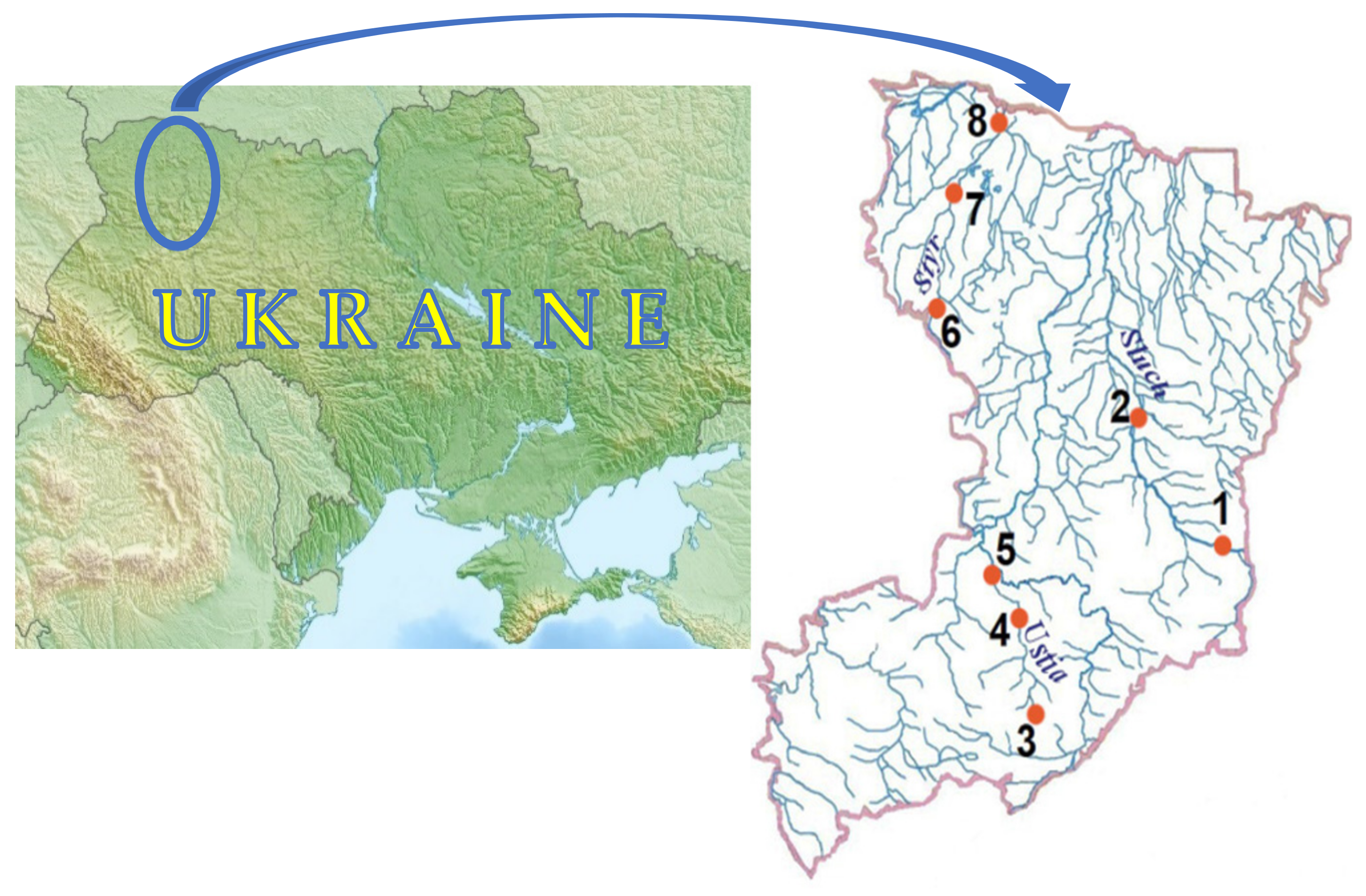
The calculated values of fluctuating asymmetry in the samples for each studied fish population in the Sluch River are shown in Table 3 and Table 4.

Thus, at both sampling site No. 1 and sampling site No. 2, the highest FFA was observed in common roach (0.42 and 0.45, respectively). The lowest FFA was found in silver crucian carp (0.13 and 0.15, respectively). The results of this study (Table 2 and Table 3) showed that the FFA was different for most of the analyzed fish populations in the Sluch River. The highest FFA for all studied fish populations was found in the gill stamens on the first gill arch (sp.br), and the lowest FFA was observed in the number of rays on the caudal fin (squ.pl).

The difference in the FFA of various fish may have been related to the impact of various factors. The generally accepted theory is that changes in fish FFA are often influenced by water quality chemistry. The value of the FFA index can also be influenced by other factors that were not studied in this research (turbidity, river depth, population density (species/m³), features of the trophic chain, etc.). The level of influence of various factors on FFA may be investigated in future studies.

The FFA results of the studied fish populations in the Ustya River are presented in Table 5, Table 6 and Table 7. At sampling site No. 3, the highest FFA values were observed in common rudd (0.40), common break (0.38), and common roach (0.36). At sampling site No. 4, the highest FFA values were found for common roach (0.53) and common bleak (0.46). At sampling site No. 5, the highest FFA values were determined for common bleak and common roach (0.48 and 0.46, respectively).

The analysis of the obtained data (Table 4, Table 5 and Table 6) showed that the highest levels of FFA were observed in the number of gill stamens on the first gill arch (sp.br.) at sampling sites Nos. 3–5 for all studied fish populations, as well as the number of rays on the pectoral fin (P) and the number of scales on the lateral line (jj).

The third studied river was the Styr River, for which the FFA results of the selected fish populations are presented in Table 8, Table 9 and Table 10. The analysis of the data presented in these tables showed that the highest FFA values at sampling site No. 6 were 0.39 for common bleak and 0.37 for common roach. The same pattern was observed at sampling site No. 7. At sampling site No. 8, the highest FFA values were 0.37 for common roach and 0.33 for common bleak. For most of the analyzed fish species at all sampling sites in this river, the highest FFA values were observed in the following features: the number of rays on the pectoral fin (P), the number of rays on the pelvic fin (V), and the number of gill stamens on the first gill arch (sp.br).

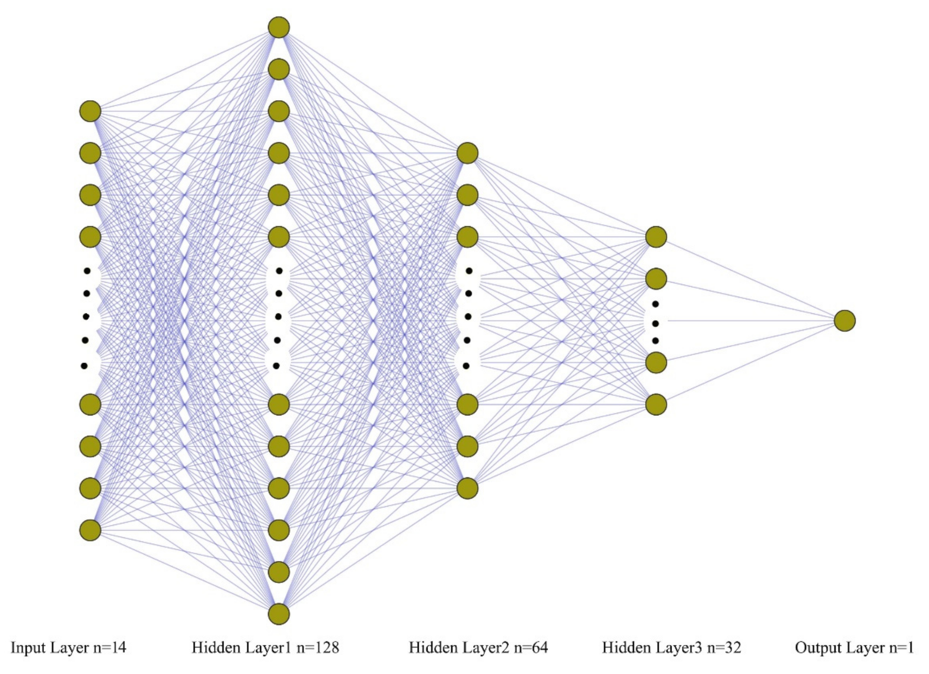
After laboratory studies, six datasets were generated that correspond to each of the six studied fish populations. The datasets were formed into matrices that contained 480 rows and 15 columns (14 columns for the input variables (SS, NH₄⁺, NO₃⁻, NO₂⁻, PO₄³⁻, BOD₅, O₂, SO₄²⁻, Cl⁻, Fe_total, Zn²⁺, Mn²⁺, FFA) and one column for the target output data (water quality)).

As an example, the creation and training of an ANN model for data obtained from a population of common bleak are shown. The database was split into three sets: training (60%), validation (20%), and testing (20%). The next step was training, validating, and testing the ANN models. The trial testing of the ANN models was carried out with the number of epochs equal to 20, 50, and 100. It was expected that the optimal values would be obtained at the level of 100 epochs. Increasing the number of epochs over 100 did not lead to an improvement in model performance.

Table 11. The parameters of the ANN models.

Parameter	Model
	ANN 1		ANN 2		ANN 3		ANN 4		ANN 5
activator	sigmoid		sigmoid		sigmoid		ReLU		ReLU
optimizer	SGD		RMSprop		ADAM		SGD		RMSprop
epochs	20	100	20	100	20	100	20	100	20	100
R2	0.91782	0.94459	0.92966	0.96611	0.90958	0.96900	0.93764	0.97187	0.89791	0.96327
MAPE, %	17.3	14.1	14.9	10.7	16.2	8.8	11.7	6.7	15.6	9.1
	ANN 6		ANN 7		ANN 8		ANN 9
activator	ReLU		tanh		tanh		tanh
optimizer	ADAM		SGD		RMSprop		ADAM
epochs	20	100	20	100	20	100	20	100
R2	0.94299	0.97627	0.97603	0.95681	0.94838	0.94538	0.94342	0.94412
MAPE, %	11.4	8.6	7.6	8.7	12.7	9.4	11.4	10.3

shows the parameters of the ANN models. The values of R² and MAPE at 20 epochs are listed for comparison purposes.

A comparative analysis of the nine neural network models showed that the ANN 4 model had the best results (with the lowest value for the average absolute error percentage and the highest value for the coefficient of determination). This neural network used the SGD optimization algorithm and the ReLU activation function. The best MAPE and R² values were obtained at the 100th epoch and were equal to 6.7% and 0.97187, respectively.

The following analysis refers to the ANN 4 model and presents an assessment of the adequacy of the results obtained and the prospects for the model’s use for forecasting with new datasets.

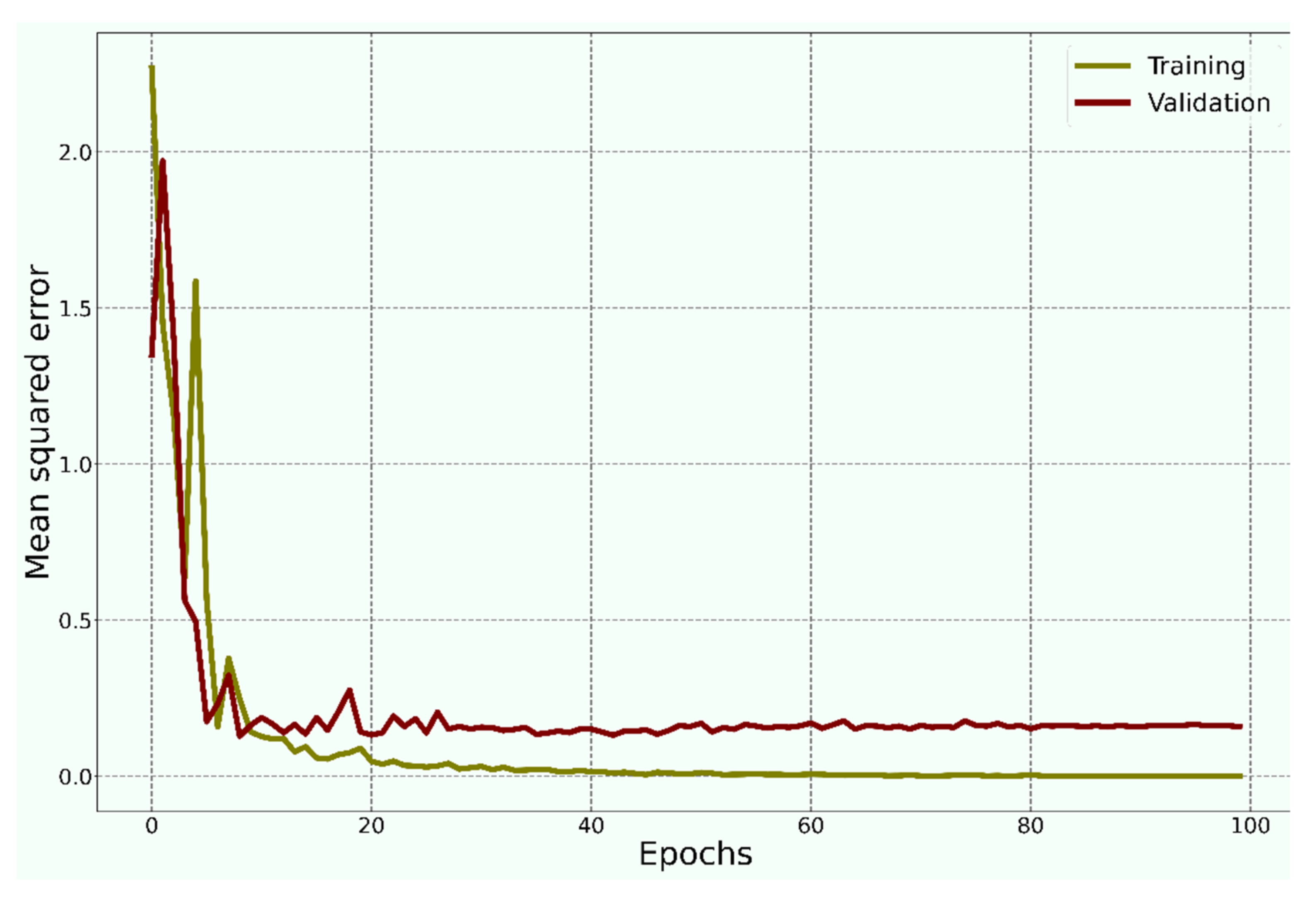
Figure 4 shows the comparison of the mean square error results for the validation and training sets. The highest MSE was obtained on the first epoch: training dataset—2.2680; validation dataset—1.3495. The lowest MSE was obtained on the 100th epoch: training dataset—0.00047; validation dataset—0.1592.

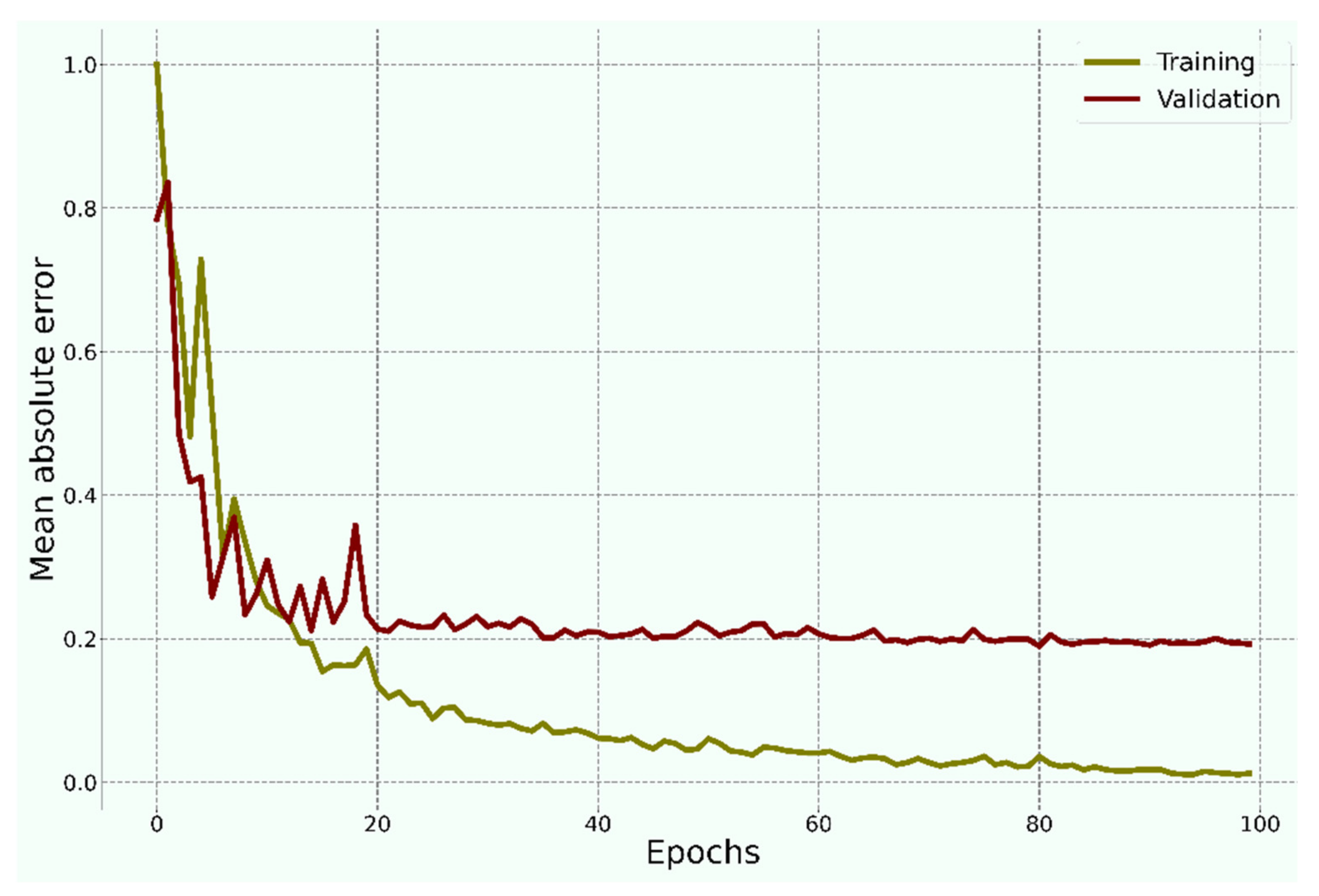
Figure 5 shows a comparison of the MAE for the validation and training sets. The highest MAE was obtained on the first epoch: training dataset—1.0000; validation dataset—0.7846. The lowest MSE was observed on the 100th epoch: training dataset—0.0125; validation dataset—0.1927.

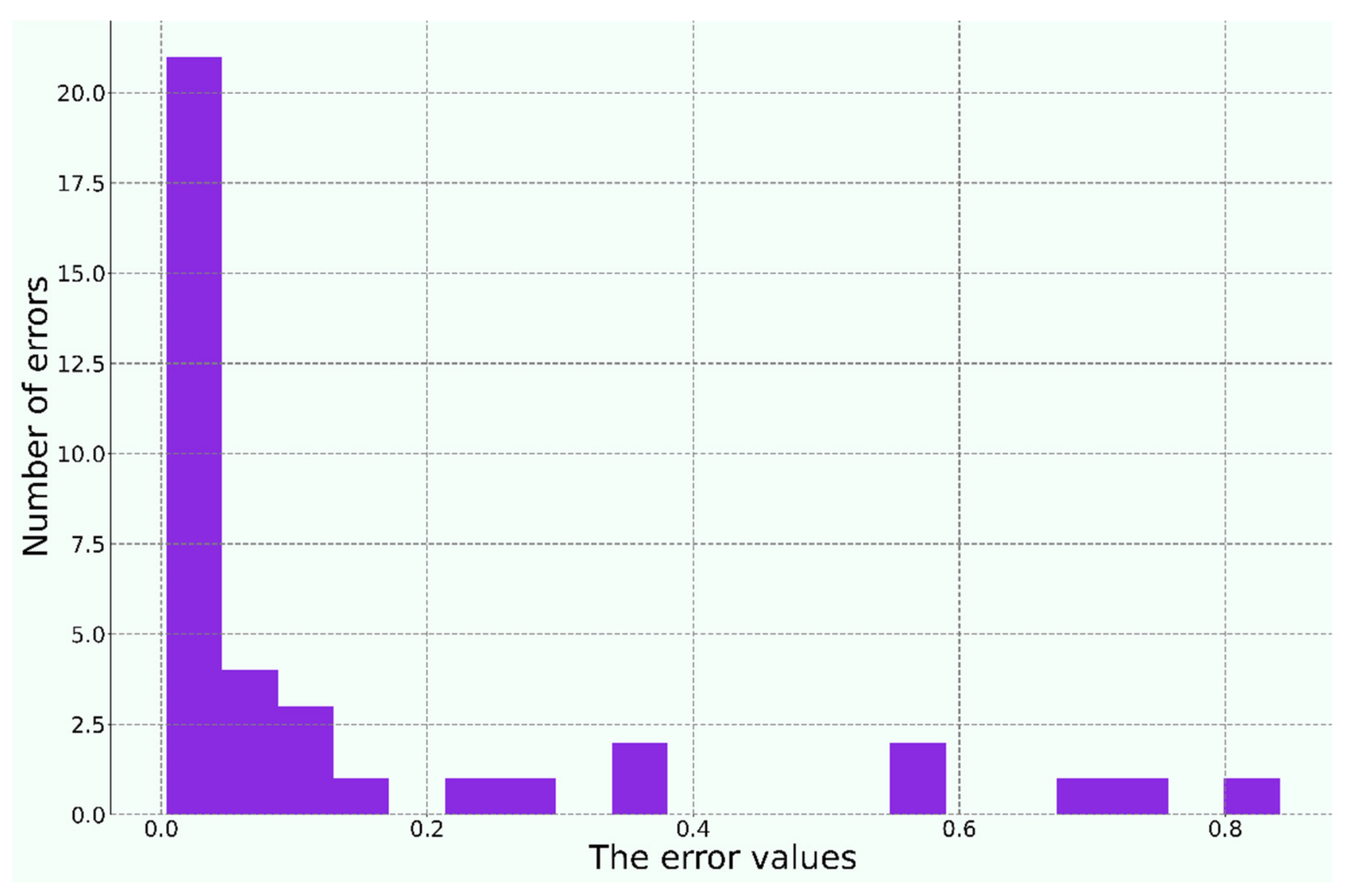
The error histogram (Figure 6) shows the distribution of data sampling errors.

According to the obtained histogram, we could conclude that the errors obeyed the normal distribution law, i.e., we could divide the errors into three regions (for simplicity, the distribution was considered to be normalized): +σ₁ → range [0.0, 0.29]; +σ₂ → range [0.3, 0.59]; +σ₃ → range [0.6, 0.89]. The vast majority of errors fell within the +σ₁ range, although there were also anomalous errors.

In their study, Rizal, Hayder, and Yusof aimed to develop artificial neural network models to predict six different water quality parameters. All the ANN models achieved high coefficients of determination (R²), which ranged from 0.9906 to 0.9998 and from 0.8797 to 0.9972 for the training and testing datasets, respectively [58].

Li et al. used a backpropagation neural network, radial basis function neural network, support vector machine, and least squares support vector machine to simulate and predict water quality parameters including dissolved oxygen, pH, ammonium-nitrogen, nitrate nitrogen, and nitrite nitrogen [59]. The results showed that the support vector machine achieved the best prediction performance, with an accuracy of 99%. This model was recommended for simulating and predicting water quality.

Khoi et al. used a case study to evaluate the performance of twelve machine learning models in estimating surface water quality [60]. The water quality index was calculated based on water quality data at four monitoring stations for the period 2010–2017. The prediction performance of the machine learning models was evaluated using two efficiency indicators (R² and RMSE). The results indicated that all twelve ML models had good performance in predicting the water quality index, but that extreme gradient boosting achieved the best performance (R² = 0.989 and RMSE = 0.107).

Thus, by comparing the error indicator and R² values of the ANN model developed in the current study (MAPE = 6.7%; R² = 0.97187) with those of models from other studies, we can state that the level of agreement between the predicted and target data was satisfactory.

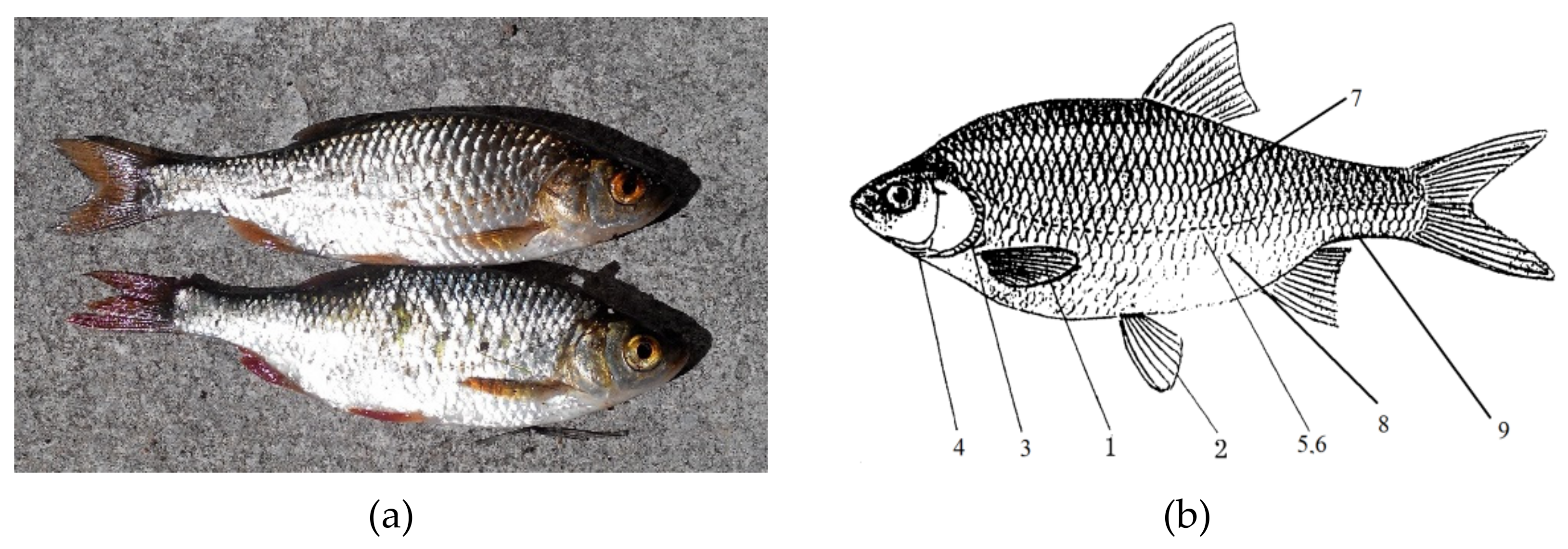
Various recent studies have shown that fish can be used as bioindicators [46,53]. The analysis of the health status of fish, their morphological traits, and other indicators is often a good monitoring tool, especially for assessing the physical and chemical pollution of surface water bodies [39,54]. At the same time, researchers have distinguished between highly sensitive fish (salmon, trout, common roach, zander, char, common bleak, and ninnow); medium-sensitivity fish (common bream, European perch, and common rudd); and low-sensitivity fish (silver crucian carp and common carp) [61,62,63,64].

A study of selected fish populations in the Sluch, Ustya, and Styr rivers showed that the highest FFA values corresponded to common roach and common bleak, and the lowest to silver crucian carp. If we compare the FFA values of these fish in the studied rivers, then common roach and common bleak had the highest values in sampling sites 3–5 of the Ustya River. This could be explained by the fact that the water quality in these sections of the river was the worst of all the studied sections. The chemical indicators of water quality that significantly exceeded their allowable levels were SS, NO₂⁻, NH₄⁺, BOD_5, Fe_total, Zn²⁺, and Mn²⁺. The excessive levels of the above indicators in the Ustya River in the period June–August suggests an active decay processes at the bottom of the reservoir. Rotting activity is associated with increased water and air temperatures in the summer. The period under study included the months, especially August, when the processes of vegetation by micro- and macrophytes are almost complete. At this time, plants cease to actively consume metals such as Fe_total, Zn²⁺, and Mn²⁺, and so their concentrations become significantly increased.

The increased content of NO₂⁻ and NH₄⁺ and the pH value of 8 indicated that the process of denitrification was taking place in the water. During the period of this study, the active growth of macrophytes was observed, causing the presence of soluble oxygen in the water. The analysis of the chemical composition of the water in the Ustya River showed that the concentration of soluble oxygen varied from 7.5 to 10.2 mgO₂/dm³. It is known that at such oxygen concentrations, the process of denitrification occurs rather slowly. Thus, the intensification of the denitrification process should not be encouraged, since a decrease in the oxygen concentration can lead to the death of all aerobic organisms.

Fish are usually found at the highest trophic level in freshwater habitats and absorb pollution from the environment they live in [65,66]. Eating contaminated fish can be a public health risk.

Töre et al. determined the probable public health risks posed by heavy metals (Mn, Cd, Fe, Cu, Ni, Zn, Co, Pb, Cr, and As) in 72 muscle and gill samples from six fish species. The highest muscle tissue levels for eight of the ten heavy metals measured were found in the C. macrostomus species. The results showed that the intake of the analyzed fish species might present a toxicological hazard and threaten community health [67]. The daily consumption of such fish could have harmful effects on human health. Therefore, the assessment of the FA level of the most popular fish species in the studied rivers is of great importance. The fish with the most pronounced FFA could serve as a biological indicator of the local situation.

In regard to the level of pollution of the Ustya River as a whole, it can be noted that at this moment the pollution is not at a critical level. However, given that this situation may change over time, it is necessary to apply the right usage policies to the river and regularly monitor its pollution parameters. The studied rivers are mainly of aesthetic and recreational value, and they are also actively used by local residents for amateur fishing.

However, for the effective management of water resources, i.e., to ensure the health of fish populations and maintain the marginal concentrations of biogenic elements and heavy metals, it is advisable to use established technological methods. In many countries, natural limestone is applied for this purpose. Adding limestone to natural surface waters can slow down the process of decay at the bottom of the reservoir. As evidenced by studies of this practice, in summer it is able to reduce the intensity of eutrophication, i.e., the concentration of PO₄³⁻ [68] and heavy metals [69]. During the dissociation of limestone, the pH value of the water increases, which makes it possible to slow down the processes of decay in the bottom of the reservoir and thus increase the aesthetic and recreational value of the river.

4. Conclusions

The object of this study was the use of fish populations as a bioindicator of water quality. The data on the dominant populations of fish in the Sluch, Ustya, and Styr Rivers were obtained from the implementation of the regional ecological program for monitoring the water quality of the Rivne region, Ukraine. Six main fish populations were identified, namely: common bream, common roach, common crucian carp, European perch, silver crucian carp, and common bream. The frequency of fluctuating asymmetry was determined for the study fish populations. Each studied fish population had a different level of fluctuating asymmetry. The highest values of FFA were observed in common roach, and the lowest values were found in silver crucian carp. It is common knowledge that the level of stress exerted on fish has an impact on the manifestations of paired meristic features (asymmetry). For freshwater fish, the main stress is the increased concentration of chemicals in water. An ANN model was developed for each selected fish population. On the basis of the determined chemical indicators of water quality in the studied rivers and the frequency of fluctuating asymmetry in the selected fish populations, an ANN model was built to predict water quality. Thus, with the help of the developed ANN model, we were able to evaluate the water quality according to the FFA values determined for samples of the investigated fish species aged below 6 months. The present research had a number of limitations; in particular, the influence of the following factors on water quality was not taken into account: geological factors, turbidity, river depth, population density (species/m³), and features of the trophic chain. Taking these limitations into account could be a direction for future research.

References

1. Birk, S.; van Kouwen, L.; Willby, N. Harmonising the Bioassessment of Large Rivers in the Absence of Near-Natural Reference Conditions—A Case Study of the Danube River: Alternative Benchmarking in Large River Bioassessment. Freshw. Biol. 2012, 57, 1716–1732. [Google Scholar] [CrossRef]
2. Krtolica, I.; Cvijanović, D.; Obradović, Đ.; Novković, M.; Milošević, D.; Savić, D.; Vojinović-Miloradov, M.; Radulović, S. Water Quality and Macrophytes in the Danube River: Artificial Neural Network Modelling. Ecol. Indic. 2021, 121, 107076. [Google Scholar] [CrossRef]
3. Milošević, D.; Mančev, D.; Čerba, D.; Stojković Piperac, M.; Popović, N.; Atanacković, A.; Đuknić, J.; Simić, V.; Paunović, M. The Potential of Chironomid Larvae-Based Metrics in the Bioassessment of Non-Wadeable Rivers. Sci. Total Environ. 2018, 616–617, 472–479. [Google Scholar] [CrossRef] [PubMed]
4. Chapman, D.V.; Bradley, C.; Gettel, G.M.; Hatvani, I.G.; Hein, T.; Kovács, J.; Liska, I.; Oliver, D.M.; Tanos, P.; Trásy, B.; et al. Developments in Water Quality Monitoring and Management in Large River Catchments Using the Danube River as an Example. Environ. Sci. Policy 2016, 64, 141–154. [Google Scholar] [CrossRef] [Green Version]
5. Vörösmarty, C.J. Global Change, the Water Cycle, and Our Search for Mauna Loa: Global Change, Water Mauna Loa. Hydrol. Process. 2002, 16, 135–139. [Google Scholar] [CrossRef]
6. Sagova-Mareckova, M.; Boenigk, J.; Bouchez, A.; Cermakova, K.; Chonova, T.; Cordier, T.; Eisendle, U.; Elersek, T.; Fazi, S.; Fleituch, T.; et al. Expanding Ecological Assessment by Integrating Microorganisms into Routine Freshwater Biomonitoring. Water Res. 2021, 191, 116767. [Google Scholar] [CrossRef]
7. Schuijt, L.M.; Peng, F.-J.; van den Berg, S.J.P.; Dingemans, M.M.L.; Van den Brink, P.J. (Eco)Toxicological Tests for Assessing Impacts of Chemical Stress to Aquatic Ecosystems: Facts, Challenges, and Future. Sci. Total Environ. 2021, 795, 148776. [Google Scholar] [CrossRef]
8. Hu, Z.; Zhang, Y.; Zhao, Y.; Xie, M.; Zhong, J.; Tu, Z.; Liu, J. A Water Quality Prediction Method Based on the Deep LSTM Network Considering Correlation in Smart Mariculture. Sensors 2019, 19, 1420. [Google Scholar] [CrossRef] [Green Version]
9. Khalil, S.; Mahnashi, M.H.; Hussain, M.; Zafar, N.; Waqar-Un-Nisa; Khan, F.S.; Afzal, U.; Shah, G.M.; Niazi, U.M.; Awais, M.; et al. Exploration and Determination of Algal Role as Bioindicator to Evaluate Water Quality—Probing Fresh Water Algae. Saudi J. Biol. Sci. 2021, 28, 5728–5737. [Google Scholar] [CrossRef]
10. Derot, J.; Jamoneau, A.; Teichert, N.; Rosebery, J.; Morin, S.; Laplace-Treyture, C. Response of Phytoplankton Traits to Environmental Variables in French Lakes: New Perspectives for Bioindication. Ecol. Indic. 2020, 108, 105659. [Google Scholar] [CrossRef]
11. Oehlmann, J.; Schulte-Oehlmann, U. Chapter 17 Molluscs as Bioindicators. In Trace Metals and Other Contaminants in the Environment; Elsevier: Amsterdam, The Netherlands, 2003; Volume 6, pp. 577–635, ISBN 978-0-08-044177-1. [Google Scholar]
12. Chovanec, A.; Hofer, R.; Schiemer, F. Chapter 18 Fish as Bioindicators. In Trace Metals and Other Contaminants in the Environment; Elsevier: Amsterdam, The Netherlands, 2003; Volume 6, pp. 639–676. [Google Scholar]
13. Łuczyńska, J.; Paszczyk, B.; Łuczyński, M.J. Fish as a Bioindicator of Heavy Metals Pollution in Aquatic Ecosystem of Pluszne Lake, Poland, and Risk Assessment for Consumer’s Health. Ecotoxicol. Environ. Saf. 2018, 153, 60–67. [Google Scholar] [CrossRef] [PubMed]
14. Ustaoğlu, F.; Tepe, Y. Water Quality and Sediment Contamination Assessment of Pazarsuyu Stream, Turkey Using Multivariate Statistical Methods and Pollution Indicators. Int. Soil Water Conserv. Res. 2019, 7, 47–56. [Google Scholar] [CrossRef]
15. Zhang, N.; Shang, G.; Dai, Y.; Zhang, Y.; Ding, S.; Gao, X. Testing the Sensitivity and Limitations of Frequently Used Aquatic Biota Indices in Temperate Mountain Streams and Plain Streams of China. Water 2021, 13, 3318. [Google Scholar] [CrossRef]
16. Wang, Q.; Li, S.; Jia, P.; Qi, C.; Ding, F. A Review of Surface Water Quality Models. Sci. World J. 2013, 2013, 231768. [Google Scholar] [CrossRef] [PubMed] [Green Version]
17. Antanasijević, D.; Pocajt, V.; Povrenović, D.; Perić-Grujić, A.; Ristić, M. Modelling of Dissolved Oxygen Content Using Artificial Neural Networks: Danube River, North Serbia, Case Study. Environ. Sci. Pollut. Res. 2013, 20, 9006–9013. [Google Scholar] [CrossRef]
18. Lin, H.; Jia, Y.; Han, F.; Xia, C.; Zhao, Q.; Zhang, J.; Li, E. Toxic Effects of Waterborne Benzylparaben on the Growth, Antioxidant Capacity and Lipid Metabolism of Nile Tilapia (Oreochromis Niloticus). Aquat. Toxicol. 2022, 248, 106197. [Google Scholar] [CrossRef]
19. Michel, M.; Tytkowska, M.; Reczek, L.; Trach, Y.; Siwiec, T. Technological Conditions for the Coagulation of Wastewater from Cosmetic Industry. J. Ecol. Eng. 2019, 20, 78–85. [Google Scholar] [CrossRef]
20. Hou, R.; Liu, C.; Gao, X.; Xu, Y.; Zha, J.; Wang, Z. Accumulation and Distribution of Organophosphate Flame Retardants (PFRs) and Their Di-Alkyl Phosphates (DAPs) Metabolites in Different Freshwater Fish from Locations around Beijing, China. Environ. Pollut. 2017, 229, 548–556. [Google Scholar] [CrossRef]
21. Varol, M.; Kaçar, E.; Sünbül, M.R.; Md Towfiqul Islam, A.R. Levels of Metals and Elements in Tissues of Fish Species in the Kızılırmak River (Turkey) and Assessment of Health Risks and Nutritional Benefits. Environ. Res. 2022, 214, 113791. [Google Scholar] [CrossRef]
22. Ali, M.M.; Ali, L.; Rakib, R.J.; Islam, S.; Bhuyan, S.; Senapathi, V.; Chung, S.Y.; Roy, P.D.; Sekar, S.; Islam, A.R.M.T.; et al. Seasonal Behavior and Accumulation of Some Toxic Metals in Commercial Fishes from Kirtankhola Tidal River of Bangladesh—A Health Risk Taxation. Chemosphere 2022, 301, 134660. [Google Scholar] [CrossRef]
23. Graham, J.H. Fluctuating Asymmetry and Developmental Instability, a Guide to Best Practice. Symmetry 2020, 13, 9. [Google Scholar] [CrossRef]
24. Dzik, J. Evolutionary Origin of Asymmetry in Early Metazoan Animals. In Advances in BioChirality; Elsevier: Amsterdam, The Netherlands, 1999; pp. 153–190. ISBN 978-0-08-043404-9. [Google Scholar]
25. Palmer, A.R. Fluctuating Asymmetry Analyses: A Primer. In Developmental Instability: Its Origins and Evolutionary Implications; Markow, T.A., Ed.; Contemporary Issues in Genetics and Evolution; Springer Netherlands: Dordrecht, The Netherlands, 1994; Volume 2, pp. 335–364. ISBN 978-94-010-4357-1. [Google Scholar]
26. Beasley, D.A.E.; Bonisoli-Alquati, A.; Mousseau, T.A. The Use of Fluctuating Asymmetry as a Measure of Environmentally Induced Developmental Instability: A Meta-Analysis. Ecol. Indic. 2013, 30, 218–226. [Google Scholar] [CrossRef]
27. Frota, G.P.; Cabrini, T.M.B.; Cardoso, R.S. Fluctuating Asymmetry of Two Crustacean Species on Fourteen Sandy Beaches of Rio de Janeiro State. Estuar. Coast. Shelf Sci. 2019, 223, 138–146. [Google Scholar] [CrossRef]
28. Seixas, L.B.; dos Santos, A.F.G.N.; dos Santos, L.N. Fluctuating Asymmetry: A Tool for Impact Assessment on Fish Populations in a Tropical Polluted Bay, Brazil. Ecol. Indic. 2016, 71, 522–532. [Google Scholar] [CrossRef]
29. Emlen, J.M.; Freeman, D.C.; Graham, J.H. Nonlinear Growth Dynamics and the Origin of Fluctuating Asymmetry. Genetica 1993, 89, 77–96. [Google Scholar] [CrossRef]
30. Gül, M.R.; Griffen, B.D. Changes in Claw Morphology of a Bioindicator Species across Habitats That Differ in Human Disturbance. Hydrobiologia 2020, 847, 3025–3037. [Google Scholar] [CrossRef]
31. Kozlov, M.V.; Zvereva, E.L. Confirmation Bias in Studies of Fluctuating Asymmetry. Ecol. Indic. 2015, 57, 293–297. [Google Scholar] [CrossRef]
32. Baş, D.; Boyacı, İ.H. Modeling and Optimization II: Comparison of Estimation Capabilities of Response Surface Methodology with Artificial Neural Networks in a Biochemical Reaction. J. Food Eng. 2007, 78, 846–854. [Google Scholar] [CrossRef]
33. Moghaddam, M.G.; Khajeh, M. Comparison of Response Surface Methodology and Artificial Neural Network in Predicting the Microwave-Assisted Extraction Procedure to Determine Zinc in Fish Muscles. FNS 2011, 2, 803–808. [Google Scholar] [CrossRef] [Green Version]
34. Zhang, G.; Eddy Patuwo, B.; Hu, Y.M. Forecasting with Artificial Neural Networks. Int. J. Forecast. 1998, 14, 35–62. [Google Scholar] [CrossRef]
35. Al-Mahallawi, K.; Mania, J.; Hani, A.; Shahrour, I. Using of Neural Networks for the Prediction of Nitrate Groundwater Contamination in Rural and Agricultural Areas. Environ. Earth Sci. 2012, 65, 917–928. [Google Scholar] [CrossRef]
36. Chen, Y.; Song, L.; Liu, Y.; Yang, L.; Li, D. A Review of the Artificial Neural Network Models for Water Quality Prediction. Appl. Sci. 2020, 10, 5776. [Google Scholar] [CrossRef]
37. Wang, T.-S.; Tan, C.-H.; Chen, L.; Tsai, Y.-C. Applying Artificial Neural Networks and Remote Sensing to Estimate Chlorophyll-a Concentration in Water Body. In Proceedings of the 2008 Second International Symposium on Intelligent Information Technology Application, Shanghai, China, 20–22 December 2008; pp. 540–544. [Google Scholar]
38. Guidance, W.C.E. Common Implementation Strategy for the Water Framework Directive (2000/60/EC); Guidance Document: Brussels, Belgium, 2009. [Google Scholar]
39. Shevchenko, P.; Pylypenko, Y. Spetsialna ikhtiolohiia. [Special Ichthyology]. Textbook in 2 Volumes; Oldi Plus: Kherson, Ukraine, 2018; Volume 1. [Google Scholar]
40. Bedunkova, O.O. Homeostasis in Fishes as an Instrument for Assessment of Critical Loads on Hydroecosystem of Small Rivers. Hydrob. J. 2016, 52, 25–33. [Google Scholar] [CrossRef]
41. Guidance, DSTU-N B V.2.3-23:2012. In Guidelines for Assessing and Predicting the Technical Condition of Road Bridges; Ministry of Regional Development and Construction of Ukraine: Kyiv, Ukraine, 2012.
42. Guidance. In Procedure for State Monitoring of Water; Guidance Document; Cabinet of Ministers of Ukraine: Kyiv, Ukraine, 2018.
43. Klymenko, M.O.; Biedunkova, O.O.; Klymenko, O.M.; Statnyk, I.I. Influence of River Water Quality on Homeostasis Characteristics of Cypriniform and Perciform Fish. Biosys. Divers. 2018, 26, 16–23. [Google Scholar] [CrossRef]
44. Van Dongen, S. Unbiased Estimation of Individual Asymmetry. J. Evol. Biol. 2000, 13, 107–112. [Google Scholar] [CrossRef]
45. Van Dongen, S.; Lens, L. The Evolutionary Potential of Developmental Instability. J. Evol. Biol. 2000, 13, 326–335. [Google Scholar] [CrossRef]
46. Van Dongen, S.; Lens, L. Symmetry, Size and Stress. Trends Ecol. Evol. 2000, 15, 330–331. [Google Scholar] [CrossRef]
47. Lens, L.; Van Dongen, S.; Matthysen, E. Fluctuating Asymmetry as an Early Warning System in the Critically Endangered Taita Thrush. Conserv. Biol. 2002, 16, 479–487. [Google Scholar] [CrossRef] [Green Version]
48. Klimenko, M.O.; Biedunkova, O.O. Development Stability and Cytogenetic Homeostasis of Perca Fluviatilis (Perciformes, Percidae) in the Rivers of Rivne Region. Vestn. Zool. 2016, 50, 539–546. [Google Scholar] [CrossRef] [Green Version]
49. Keller, J.M. Fundamentals of Computational Intelligence: Neural Networks, Fuzzy Systems, and Evolutionary Computation; IEEE Press Series on Computational Intelligence; IEEE Press/Wiley: Hoboken, NJ, USA, 2016; ISBN 978-1-119-21434-2. [Google Scholar]
50. Kalenik, M.; Chalecki, M. Experimental Study of Air Lift Pump Delivery Rate. Rocz. Ochr. Srodowiska 2018, 20, 221–240. [Google Scholar]
51. Trach, R.; Trach, Y.; Lendo-Siwicka, M. Using ANN to Predict the Impact of Communication Factors on the Rework Cost in Construction Projects. Energies 2021, 14, 4376. [Google Scholar] [CrossRef]
52. Ruder, S. An Overview of Gradient Descent Optimization Algorithms. arXiv 2017, arXiv:1609.04747. [Google Scholar]
53. Kingma, D.P.; Ba, J. Adam: A Method for Stochastic Optimization. arXiv 2017, arXiv:1412.6980 [cs]. [Google Scholar]
54. Kowalski, J.; Połoński, M.; Lendo-Siwicka, M.; Trach, R.; Wrzesiński, G. Method of Assessing the Risk of Implementing Railway Investments in Terms of the Cost of Their Implementation. Sustainability 2021, 13, 13085. [Google Scholar] [CrossRef]
55. Kalenik, M.; Chalecki, M. Investigations on the Effectiveness of Wastewater Purification in Medium Sand with Assisting Opoka Rock Layer. Environ. Protect. Eng. 2021, 47, 53–65. [Google Scholar] [CrossRef]
56. Trach, Y.; Trach, R.; Kalenik, M.; Koda, E.; Podlasek, A. A Study of Dispersed, Thermally Activated Limestone from Ukraine for the Safe Liming of Water Using ANN Models. Energies 2021, 14, 8377. [Google Scholar] [CrossRef]
57. Trach, R.; Trach, Y.; Kiersnowska, A.; Markiewicz, A.; Lendo-Siwicka, M.; Rusakov, K. A Study of Assessment and Prediction of Water Quality Index Using Fuzzy Logic and ANN Models. Sustainability 2022, 14, 5656. [Google Scholar] [CrossRef]
58. Rizal, N.N.M.; Hayder, G.; Yusof, K.A. Water Quality Predictive Analytics Using an Artificial Neural Network with a Graphical User Interface. Water 2022, 14, 1221. [Google Scholar] [CrossRef]
59. Li, T.; Lu, J.; Wu, J.; Zhang, Z.; Chen, L. Predicting Aquaculture Water Quality Using Machine Learning Approaches. Water 2022, 14, 2836. [Google Scholar] [CrossRef]
60. Khoi, D.N.; Quan, N.T.; Linh, D.Q.; Nhi, P.T.T.; Thuy, N.T.D. Using Machine Learning Models for Predicting the Water Quality Index in the La Buong River, Vietnam. Water 2022, 14, 1552. [Google Scholar] [CrossRef]
61. Klimenko, N.A.; Pylypenko, Y.V.; Biedunkova, O.O. Health Assessment of Hydro-Ecosystems Based on Homeostasis Indicators of Fish: Review of Approaches. Biosys. Divers. 2016, 24, 61–71. [Google Scholar] [CrossRef]
62. Hallam, T.G.; Lika, K. Modeling the Effects of Toxicants on a Fish Population in a Spatially Heterogeneous Environment: I. Behavior of the Unstressed, Spatial Model. Nonlinear Anal. Theory Methods Appl. 1997, 30, 1699–1707. [Google Scholar] [CrossRef]
63. Kubečka, J.; Boukal, D.S.; Čech, M.; Hickley, P.; Kitchell, J.F.; Ricard, D.; Rudstam, L.; Soukalová, K.; Welcomme, R. Ecology and Ecological Quality of Fish in Lakes and Reservoirs. Fish. Res. 2016, 173, 1–3. [Google Scholar] [CrossRef]
64. Greenstreet, S.P.R.; Rossberg, A.G.; Fox, C.J.; Le Quesne, W.J.F.; Blasdale, T.; Boulcott, P.; Mitchell, I.; Millar, C.; MoFFAt, C.F. Demersal Fish Biodiversity: Species-Level Indicators and Trends-Based Targets for the Marine Strategy Framework Directive. ICES J. Mar. Sci. 2012, 69, 1789–1801. [Google Scholar] [CrossRef] [Green Version]
65. Ali, M.M.; Ali, M.L.; Proshad, R.; Islam, S.; Rahman, Z.; Kormoker, T. Assessment of Trace Elements in the Demersal Fishes of a Coastal River in Bangladesh: A Public Health Concern. Thalassas 2020, 36, 641–655. [Google Scholar] [CrossRef]
66. Ustaoğlu, F.; Taş, B.; Tepe, Y.; Topaldemir, H. Comprehensive Assessment of Water Quality and Associated Health Risk by Using Physicochemical Quality Indices and Multivariate Analysis in Terme River, Turkey. Environ. Sci. Pollut. Res. 2021, 28, 62736–62754. [Google Scholar] [CrossRef]
67. Töre, Y.; Ustaoğlu, F.; Tepe, Y.; Kalipci, E. Levels of Toxic Metals in Edible Fish Species of the Tigris River (Turkey); Threat to Public Health. Ecol. Indic. 2021, 123, 107361. [Google Scholar] [CrossRef]
68. Yanamadala, V. Calcium Carbonate Phosphate Binding Ion Exchange Filtration and Accelerated Denitrification Improve Public Health Standards and Combat Eutrophication in Aquatic Ecosystems. Water Environ. Res. 2005, 77, 3003–3012. [Google Scholar] [CrossRef] [Green Version]
69. Davis, A.D.; Webb, C.J.; Sorensen, J.L.; Dixon, D.J.; Hudson, R. Geochemical Thermodynamics of Cadmium Removal from Water with Limestone. Environ. Earth Sci. 2018, 77, 37. [Google Scholar] [CrossRef]
Figure 1. Map and scheme of the water and fish sampling sites (numbers 1–8 are observation posts).
Water 14 03511 g001
Figure 2. (a) appearance of caught common roach; (b) diagram of meristic features of fish. Adapted with permission from Ref. [40].
Water 14 03511 g002
Figure 3. The structure of the neural network.
Water 14 03511 g003
Figure 4. The MSE values for training and validation datasets.
Water 14 03511 g004
Figure 5. The MAE values for training and validation datasets.
Water 14 03511 g005
Figure 6. Error histogram.
Water 14 03511 g006