Article

A Continuous Multisite Multivariate Generator for Daily Temperature Conditioned by Precipitation Occurrence

by
Joel Hernández-Bedolla
1,
Abel Solera
2,
Javier Paredes-Arquiola
2,
Sonia Tatiana Sanchez-Quispe
1,* and
Constantino Domínguez-Sánchez
1
1
Faculty of Civil Engineering, Michoacan University of Saint Nicolas of Hidalgo, Morelia 58030, Mexico
2
Research Institute of Water and Environmental Engineering (IIAMA), Universitat Politècnica de València, 46022 Valencia, Spain
*
Author to whom correspondence should be addressed.
Water 2022, 14(21), 3494; https://doi.org/10.3390/w14213494
Submission received: 11 September 2022 / Revised: 16 October 2022 / Accepted: 24 October 2022 / Published: 1 November 2022

Abstract

:
Temperature is one of the most influential weather variables necessary for numerous studies, such as climate change, integrated water resources management, and water scarcity, among others. The temperature and precipitation are relevant in river basins because they may be particularly affected by modifications in the variability, for example, due to climate change. We developed a stochastic model for daily precipitation occurrences and their influence on maximum and minimum temperatures with a straightforward approach. The Markov model has been used to determine everyday occurrences of rainfall. Moreover, we developed a multisite multivariate autoregressive model to represent the short-term memory of daily temperature, called MASCV. The reduction of parameters is an essential factor addressed in this approach. For this reason, the normalization of the temperatures was performed through different nonparametric transformations. The case study is the Jucar River Basin in Spain. The multisite multivariate stochastic model of two states and a lag-one accurately represents both occurrences as well as maximum and minimum temperature. The simulation and generation of occurrences and temperature is considered a continuous multivariate stochastic process. Additionally, time series of multiple correlated climate variables are completed. Therefore, we simplify the complexity and reduce the computational time for the simulation.

1. Introduction

The stochastic modeling approach has been widely used for hydrologic time series analysis, including modeling weather variables [1,2] and flood prediction [3]. Therefore, it is essential to build accurate forecast models in the hydrologic process [4]. The stochastic modeling of temperature conditioned by precipitation is proposed when a day is wet or dry. It is necessary to estimate the temperature for both dry and wet days.
The most common stochastic model is the first-order Markov model with two states. It was introduced by Gabriel and Newman [5] and has since been used and modified by many authors [3,4,5,6,7,8,9,10,11,12,13,14,15,16,17,18,19]. The rainfall occurrence process focuses on representing the dry and wet days. Critical probability ( p c ) depends on transition probabilities of dry–wet ( p 01 ) and wet–wet days ( p 11 ) [8]. Thus, the occurrence is a bivariate function (0,1) that relies on the uniform random process ( u ) and critical probabilities [12].
The temperature displays a near-normal distribution. It is common to consider the normal distribution to minimize the skewness coefficient of observed data. In other cases, root transformation is used [20].
The statistical characteristics of the series change throughout the whole year. The mean, variance, and standard deviation are periodic—these statistical changes are yearly, monthly, daily, and even hourly. This periodicity is commonly modeled by the finite Fourier series [9,16,21,22]. The periodic component is necessary for standardization, which is a process that converts into a series with a mean of zero and a standard deviation of one. Standardization is usually applied to series with no follow-up normal distributions [7,23,24,25]. Moreover, standardization helps remove the seasonal effects [26]. Standardized series are used to calculate the autoregressive parameters of the stochastic model [27].
It is desirable to generate synthetic temperature based on weather data [9]. The process should be capable of representing different statistics from historical data [18]. The basic statistics of the series are the sample mean, standard deviation, skewness coefficient, cross-correlation coefficients, and probability distribution. We must fit a probability distribution function (two or more parameters) or use a nonparametric transformation. Many authors have proposed stochastic weather generators (WG) for different purposes, a few of which are downscaling, prediction, or simulation [28]. Some developed models are Weather GENerator (WGEN) [29], CLImate GENerator (CLIGEN) [30], Agriculture and Agri-Food Canada Weather Generator (AAA-FC) [27], CLIMate GENerator (CLIMGEN) [31], Long Ashton Research Station-Weather Generator (LARS-WG) [21], the weather generator CLIMA [32], the closed skew-normal weather generator (WACS-Gen) [26], École de technologie supérieure Weather Generator (WeaGETS) [22], and the Multi-site Rainfall Simulator (MRS) [18]. We propose the multivariate autoregressive model of climate variables (MASCV).
For precipitation, weather generators analyze the occurrence similarly. For example, CLIMA [32], CLIGEN [30], and WGEN [9] model the occurrence process based on transition probabilities of lag-one and two states for each month (two parameters). LARS-WG [21] is based on an empirical function of wet and dry days for each month (21 parameters). CLIMGEN [31] models the occurrence process through transition probabilities of a second-order Markov model at a monthly scale (four parameters). WeaGETS [22] models the transition probabilities of a third-order Markov model with two states on a biweekly scale (eight parameters). WASC-Gen uses a lag-one Markov model with different states and parameters derived from the Bayesian information criterion [26]. AA-FC-WG models the occurrence process with a second-order Markov model at a monthly scale using two parameters [27]. Other stochastic models have proposed modifications or new methods, such as the Markov renewal model [33], Copula-based models [34], the Hidden Markov model [35,36], the Semi-Markov model [37], generalized chain-dependent process models [38], the autoregressive model [39], and artificial intelligence [40].
Artificial intelligence (AI) has been used to predict hydrological data, including rainfall, rainfall runoff, and temperature [4]. Various machine learning methods have been applied for rainfall and temperature prediction, such as the support vector machine (SVM) classifier [41], ANN [42], long short-term memory (LSTM), statistical and multiple linear regression (MLR) [43,44], and classification and regression trees [45].
Stochastic weather generators are used to represent different variables such as precipitation and temperature. Long temperature series are commonly required, but historical data are sometimes short in length. Therefore, it is necessary to apply stochastic weather generators for hydrological design [12]. The integrated water resources management (IWRM) depends on water availability [46]. For the hydric balance and various decisions at a river basin scale, the rainfall is fundamental [10], primarily to generate long synthetic series.
The issue with synthetic series is preserving the low-frequency variability in temperature and rainfall [47]. Daily temperature series have a strong correlation [48]. To preserve low-frequency variability, different authors have proposed the fast Fourier transform (FFT) algorithm [49], using crop variables [50], annual and monthly autoregressive models [51], k-nearest neighbor bootstrap [52], and the copulas approach [53].
The objective of this paper was to develop an adequate stochastic model for daily maximum and minimum temperature with a straightforward approach. We propose a multisite multivariate stochastic model for precipitation occurrences and temperature capable of reproducing spatial and temporal dependence. We corrected the daily stochastic model using an annual multisite multivariate autoregressive model. For precipitation, we applied a multivariate multisite lag-one Markov model with two states (wet and dry) and few parameters. A normal distribution was used to define the precipitation occurrence process. For the maximum and minimum temperature, we implemented the first-order multisite multivariate autoregressive model (MAR(p)) for daily and annual temperature. Our approach simplifies the temperature simulation (continuous and nonparametric), which implies a considerable advantage and versatility concerning other stochastic generators (parametric distribution function for each month or biweekly).
The normalized mean and variance periodicity was modeled as a continuous daily scale through the Fourier series. The model validation was performed by synthetic series of precipitation, which accurately represent the main statistics of observed data for different climates. MASCV was programmed in MATLAB and is capable of simulating with various parameters for both occurrences and temperature. Moreover, we proposed a multisite multivariate stochastic model in which different wet thresholds and nonparametric transformations can be applied. A relevant advantage is that we modeled continuously for the whole series. The method developed in this paper generates constant day-to-day rainfall occurrences and temperature.

2. Materials and Methods

The purpose of generating long series of temperatures is to evaluate the effects of hydrologic changes [4,9] and analyze different scenarios, such as environmental, agricultural [28], or climate change. We focused on developing long multivariate synthetic series of maximum and minimum temperature. The lag-one Markov model has been applied for plenty of weather modelers due to its accurate representation of dependence [12]. Said model is based on terms of occurrence given the previous day. We modeled the rainfall occurrence and the temperature separately (Figure 1), so we defined the model according to Equation (1):
Y t = T t X t
where T t is the temperature model, X t is the precipitation occurrence model, and Y t is the whole stochastic process.

2.1. Multivariate Precipitation Occurrence (Dry–Wet)

First, we must determine whether a day is wet or dry according to the day prior. We used a bivariate function ( X t ), and if the precipitation is greater than a given threshold, the t day is wet ( X t = 1 ); otherwise, the t day is dry ( X t = 0 ) . The first-order Markovian approach only depends on the previous day, whether it was wet or dry. The high-order Markov model has been notably studied [54,55] and is recommended for vast persistence [10]. The two- and three-order Markov models significantly improve the fit [22,56,57]. In other cases, the results are nearly equivalent to the first-order Markov model [54]. One disadvantage of the high-order Markov model is the increase in the number of parameters [28]. The threshold for precipitation occurrence could change according to different data. This depends on the minimum value of precipitation amount that the station in the study can report. Common threshold values are 0 [9,21,29,30], 0. [22,26,58], 0.2 [25], 0.254, and 0.3 mm [18]. We used the wet thresholds (0.001, 0.01, 0.1, and 0.25) and identified the ones that provided the best results. A disadvantage in the case of stochastic modeling is the limited data from the historical period.
For the occurrence process, we used the Wilks approach [12]. The conditional probabilities for a one-order Markov model are a dry day followed by a wet day, p 01 , a wet day followed by a wet day, p 11 , a wet day followed by a dry day, p 10 , and a dry day followed by a dry day, p 00 . The conditional probabilities have a complementary relationship between them.
The normal critical probability ( p c ) depends on the previous day ( X t 1 ) ; if it is dry, p c = p 01 , otherwise p c = p 11 . The boundary for the precipitation occurrence process is determined for a random spatially correlated normal matrix n t = 1 u t   [ 0 , 1 ] . Only one day is computed if the random variable is equal to or less than a critical probability.
i f n t     p c     X t = 1 ;    n t > p c     X t = 0
The transition probability vectors vary on a monthly and daily scale. Therefore, the occurrence process was simulated through different parameters. The lag-one Markov model with two states enables the interaction between wet and dry days. Moreover, it allows the residence time and periodicity in both the first (dry) and second (wet) states.
For the daily occurrence process, one of the disadvantages is the limited number of data, primarily for dry seasons and arid river basins. These data limit the quality of results, and it is common to model the transition probabilities monthly or biweekly [9,22,26,27,30,31].
Our approach was to simulate the transition probabilities on a daily scale, similar to Woolhiser and Pegram [59]. It is imperative to preserve most of the characteristics for days, months, and years. The number of parameters increases from a monthly to a daily scale; therefore, it is essential to determine the most efficient model. In this study, we focused on the relevance of evaluating different analyses, which depend on the number of parameters, p 01 τ =   P 01 | τ and p 01 τ = P 11 | τ .
Due to the distinct temporal scales of analysis, the number of parameters will increase according to the variability of the occurrence process. The transition probabilities follow a uniform distribution applicable in the case of univariate modeling. However, in the case of multivariate modeling, a transformation to the normal distribution is more efficient [15]. A transformation was performed from uniform to normal, p n 11 τ = 1 ( p 11 τ )   and   p n 01 τ = 1   ( p 01 τ ) . The spatial correlation between probability vectors with lag-k is shown in Equation (3):
r k ( i , j ) ( p ) = ( p n 11 ( i , j ) p n 01 ( i , j ) ) k i j
where r k ( i , j ) is the spatial correlation with lag-k, p n 11 ( i , j ) is the normalized probability vector of two consecutive days of rainfall occurrence, and p n 01 ( i , j ) is the normalized probability vector of a dry day followed by a wet day. Based on these vectors, a spatially correlated matrix was proposed in Equation (4):
M k = [ r k ( 1 , 1 ) ( p ) r k ( 1 , n ) ( p ) r k ( n , 1 ) ( p ) r k ( n , n ) ( p ) ]
where M k is the cross-correlation matrix. The Cholesky factorization was used to determine the spatial dependence of the series [15,19,60]. For a positive definite matrix, the Cholesky factorization is a lower triangular matrix, D = [ M ] [ M ] . Multiplying this lower triangular matrix by a random normal matrix results in a random spatially correlated normal matrix, n, in Equation (5):
n = [ M ] [ N ] = [ M ( 1 , 1 ) 0 M ( n , 1 ) M ( n , n ) ] x [ N ( 1 , 1 ) N ( 1 , m ) N ( n , 1 ) N ( n , m ) ]
where n is the random spatially correlated normal matrix, M ( n , n ) is the lower triangular matrix for n series, and N ( n , m ) is the random normal matrix for n series and m days. We used this matrix to generate multivariate precipitation occurrences. In addition, they were used to determine synthetic wet and dry days.

2.2. Multivariate Maximum and Minimum Temperature

The maximum and minimum temperatures were modeled using the original maximum temperature data and the difference between the maximum and minimum temperature, Trange in Equation (6). The target of modeling the temperature range is to avoid negative values of the synthetic series [61].
T r a n g e = T m a x T m i n
The temperature process is commonly modeled considering normal distribution. However, according to our experience, in some cases, the maximum temperature and temperature range follow a normal distribution. We focused on the nonparametric transformations. These are practical solutions to model the temperature [25,56,62].
Seasonal variability is one of the most significant characteristics of the stochastic temperature process. The daily temperature shows recurrent changes within the year. Parameters such as the mean and standard deviation are periodic components [1]. The periodicity was analyzed through the Fourier series [59]. The number of parameters is reduced when these are periodic or seasonal. The Fourier series [23,59] is present in Equation (7). Several harmonics were used to represent 90% of the explicative variance of the observed data.
v = u ¯ + j = 1 h [ A j cos ( 2 π τ w ) + B j sin ( 2 π τ w ) ]
where u ¯ is the normalized temperature mean for wet ( μ 1 τ ) and dry days ( μ 0 τ ) and standard deviation for wet ( s 1 τ ) and dry days ( s 0 τ ). A and B are the Fourier coefficient vectors, j is the harmonic, and h is the total number of harmonics, equal to (w − 1)/2 for even numbers and equal to w/2 for uneven numbers. For example, in a daily simulation, we have 365 days, and the maximum number of harmonics is 182. Important harmonics were selected according to the accumulated period-gram, defined as the ratio of mean standard deviation (MSD) of the harmonics to the observed series. We accepted 90% of the original data representation to select the significant harmonics applied at the mean, standard deviation, and transition probabilities ( μ 1 τ ,   μ 0 τ ,   s 1 τ ,   s 0 τ ,   p 01 τ ,   p 11 τ ).
Once the periodic component was modeled, we standardized both temperatures (maximum and range), allowing the analysis of temporal dependence. In addition, a standardized series served to generate residual series. Standardization removes the periodicity of the series based on the mean ( μ 1 τ , μ 0 τ ) and standard deviation ( s 1 τ ,   s 0 τ ). We determined the standardized series ( z τ ) at a daily scale, canceling the mean and standard deviation of the normalized series according to Equation (8):
z τ = y τ μ 0 τ s 0 τ ;       y τ = 0 ;           z τ = y τ μ 1 τ s 1 τ         y τ > 0 ;
A multivariate autoregressive model, MAR(1), with constant parameters was applied, in which the best fit needs to represent the conditions of temporal and spatial dependence. The first order of the multivariate autoregressive model was determined based on the Cholesky factorization. In the same way, temporal dependence was conditioned by precipitation occurrence in Equation (9):
[ ϕ ] 1 = M 0 M 1 ;   [ ϕ ] 0 [ ϕ ] 0 T = M 0 [ ϕ ] 1 M 1 T ;   [ ϕ ] 0 [ ϕ ] 0 T = D
where [ ϕ ] 1 is the lag 1 autoregressive coefficient matrix, [ ϕ ] 0 is the lag 0 autoregressive coefficient matrix, [ ϕ ] 0 T is the transposed matrix, M 0 and M 1 are the cross-correlation matrices, and D is the positive definite matrix. Finally, we determined the white noise based on the multivariate autoregressive coefficient matrix using Equation (10):
ε τ = [ ϕ ] 0 1 ( { z } τ [ ϕ ] 1 { z } τ 1 )

2.3. Evidence for the Goodness of Fit

The residual series must satisfy the residual normality ( ε 0 ,   s ε 1 ), which is neither correlated ( r k ( ε ) 0 ) nor has a biased judgment ( g ε 0 ) . The probability of the residual series is verified by the confidence interval limits as well as for the mean, skewness coefficient, standard deviation, and correlations to corroborate the residual series normality. It must satisfy the mean and correlation of the entire series within 95% of the confidence limits [63]. In the case of the standard deviation of the chi-squared test, it should comply with a 95% confidence for a normal distribution [64]. The skewness coefficient of the residual series must be within the confidence limits [63]. Another evaluated aspect in the stochastic process is the Akaike information criterion (AIC) [65].

2.4. Generation of Multivariate Synthetic Series
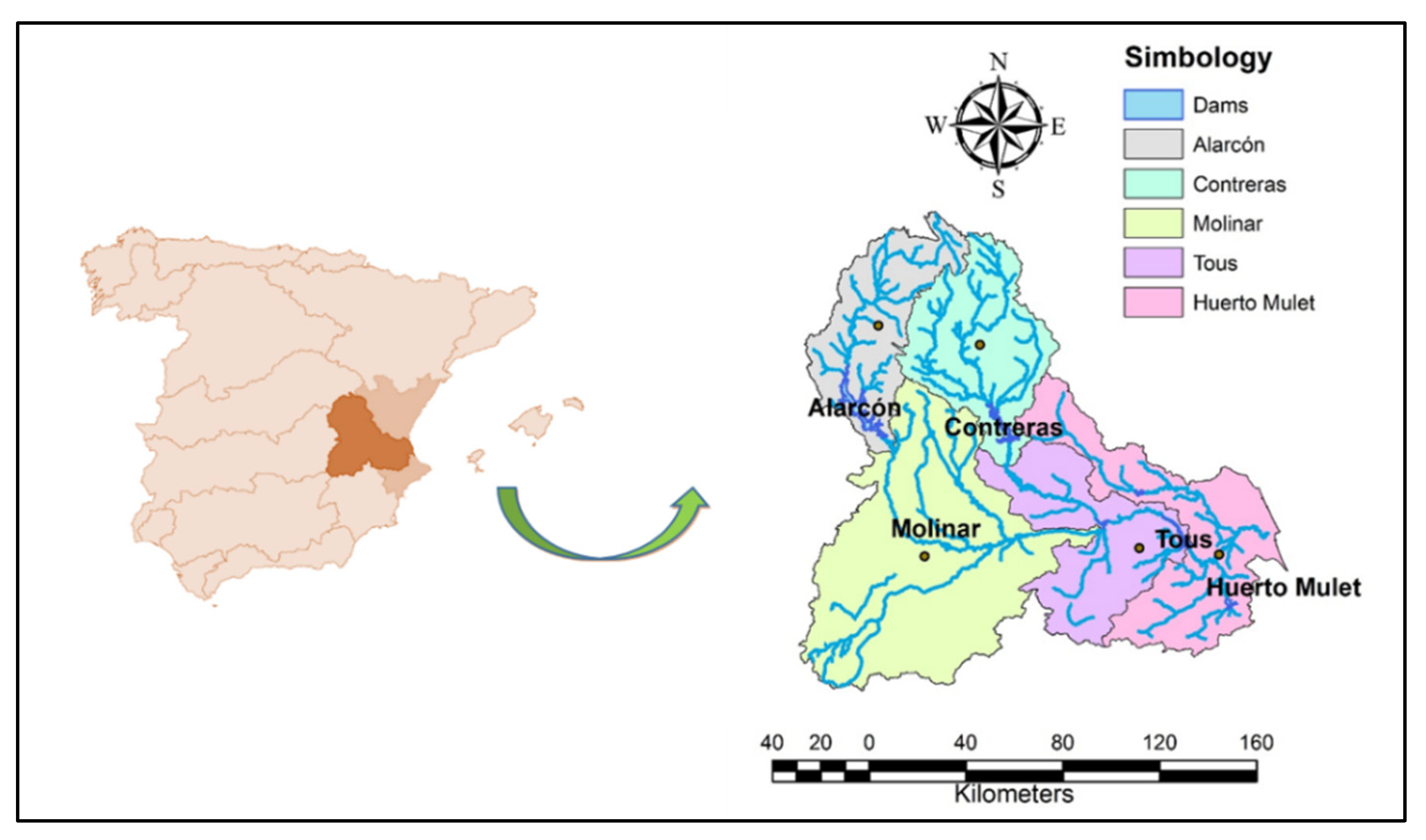
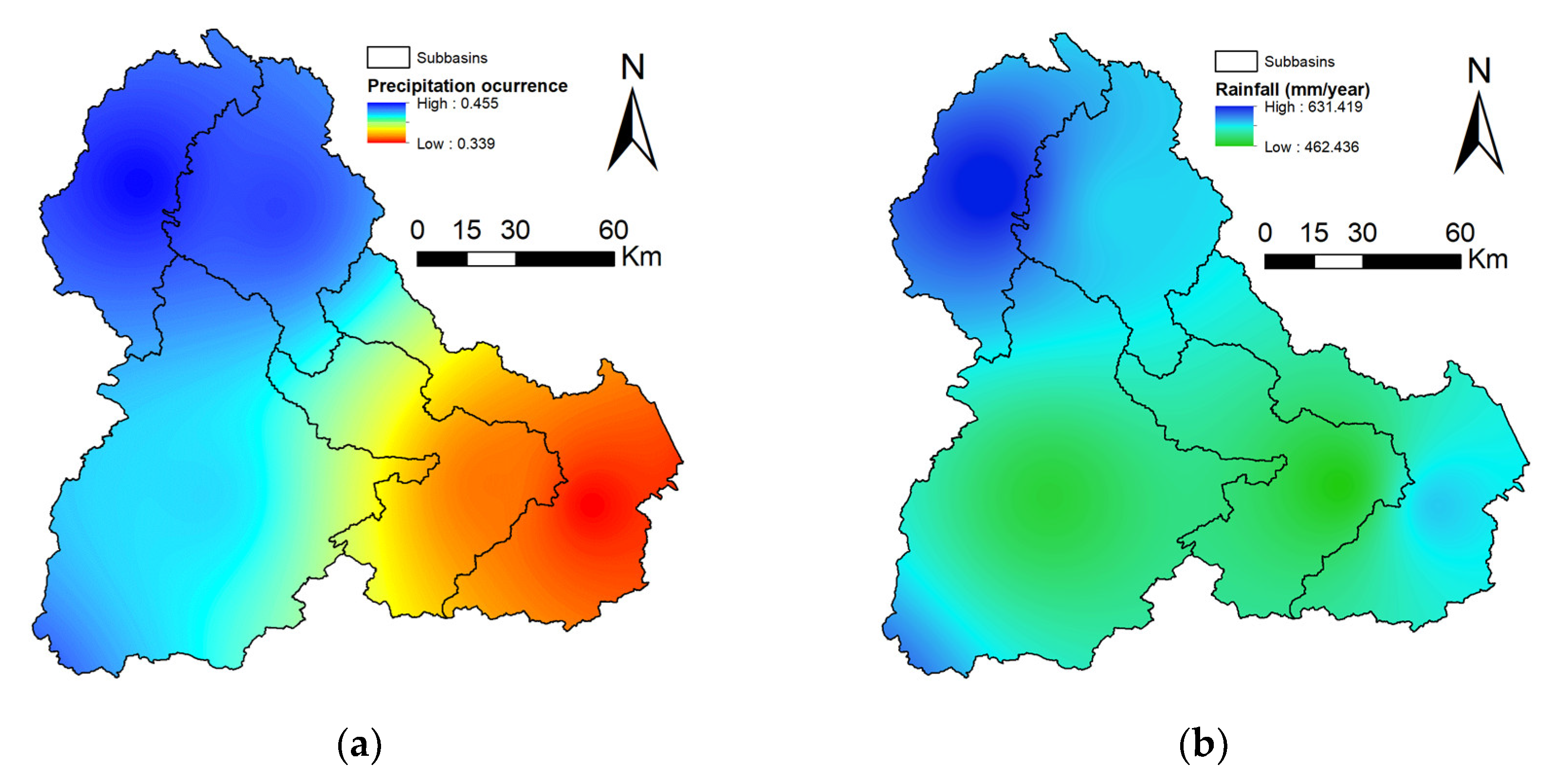
For the generation of synthetic series, the stochastic model is divided into two states, the precipitation occurrence ( X t ) and the maximum temperature and temperature range ( T t ) . The precipitation occurrence will appear if the transition vector ( p c ) is a random normally distributed number greater than the random normal distribution ( n t ) ; in other words, if n t     p c , it reaches the wet state. The stochastic temperature process starts by generating a random number with a normal distribution ( ε ) and then obtains the coupled standardized series ( z t ) and corrected using the annual low-frequency multivariate stochastic model. Finally, the inverse normalization ( y τ 1 ) was used.
The obtainment of synthetic series through the stochastic process allows for validating the developed model. The multivariate series were generated with the same characteristics as the observed data. The statistical parameters of both series were assessed and should not be significantly different; consequently, the developed model can be validated. The main metrics were determined. Mean absolute error (MAE), root mean square error (RMSE), and percent error estimate (PE) were defined.

2.5. Study Area

The Jucar River Basin is part of the Jucar Basin Agency (JBA), located in the eastern portion of the Iberian Peninsula, Spain. The basin covers an area of approximately 22,291 km2. Information regarding the zone was obtained from the official website of the confederation (www.chj.es). The most relevant surface runoff is the Jucar River, which captures the surface runoff of all sub-basins [66]. The most significant reservoirs are Alarcon (1088 hm3) and Contreras (852 hm3). The river rises from the Tragacete (1600 ms.n.m) and subsequently arrives at reservoirs Toba, Alarcon, Molinar, and Tous. The study area’s limit ends where the Mediterranean Sea is reached (Figure 2). Rainfall in the Jucar River Basin has decreased since 1980 [67,68]. Temporal and spatial variation characteristics of meteorological elements in the Jucar River Basin are presented in Appendix A (Figure A1, Figure A2, Figure A3 and Figure A4).
The Jucar River Basin is divided into five sub-basins: Alarcon, Contreras, Molinar, Tous, and Huerto Mulet. The precipitation data for the study area were obtained from the Spain 02 database [69], a regular grid (20 × 20 km). The historical data have information from 1950 to 2015. The observed data were interpolated using the inverse distance weighting (IDW) method to generate a rainfall and temperature series for each sub-basin. The IDW method is one of the most common interpolation techniques [46,70,71,72].

3. Results

According to the information of the Jucar River Basin, the average annual temperature was between 17.5 °C (Contreras) and 21 °C for the years 1950–2015. In the present study, we defined four wet day thresholds (0.001, 0.01, 0.1, and 0.25 mm). The range of rainy days from October to May was between 7.3 and 12.17, and for June to September, the average precipitation occurrences were between 2.4 and 8.72 days. The months with few precipitation occurrences were between June and September, an important factor because there were little data for the stochastic modeling process. In the case of the months from October to May, the information was essential for the stochastic modeling to perform with better confidence.

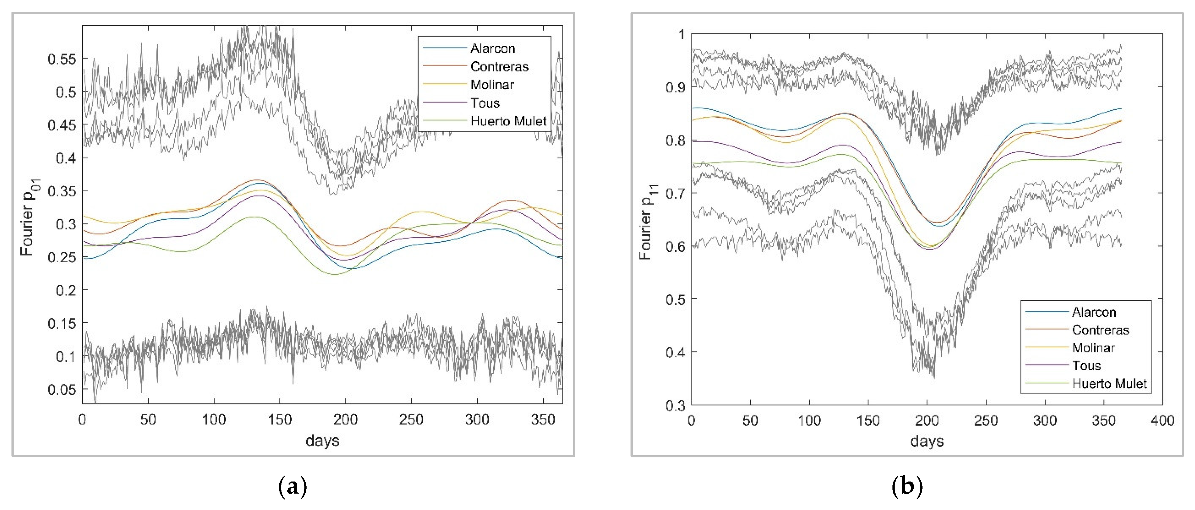
3.1. Multivariate Occurrence Synthetic Series

The occurrence process was developed through a Markov model of two states. The transition probability vectors were identified, and the daily noise level can be observed. The transition probabilities for all sub-basins p 01 τ were in a range of 0.05 (minimum) to 0.45 (maximum). On the other hand, the transition probabilities p 11 τ were between 0.3 and 0.95 (according to Figure 3).
The transition vectors were evaluated with four parameters for the Fourier series. The objective of analyzing the transition probability vectors was to select the best representation of the wet–dry event. Simulations were carried out from two harmonics in the Fourier series to reach approximately 90% of the explicative variance. However, the process of rainfall occurrence can be represented by only a few parameters [9,22,29,73]; therefore, using few harmonics is acceptable. The frequency of the precipitation for four parameters represents a smoothed probability of occurrences, and with these few parameters, a good approximation of p 11 τ and p 01 τ can be obtained (Figure 3). On the other hand, the confidence limits for the vectors p 11 τ and p 01 τ were determined from the approximation to the t-distribution with 95% confidence. For the Fourier probability p 01 τ , four main patterns were observed, predominantly the Fourier probability increase in March, April, and May, after a decrease in June and July, an increase again in August and September, and finally, from October to February, the smoothed Fourier probabilities were nearly constant. A similar pattern was present for the Fourier probability p 11 τ , which had no considerable fluctuations between October and May, decreases in June and July, and increases once more in August and September. These Fourier series are sufficient for proper stochastic performance of rainfall occurrence.

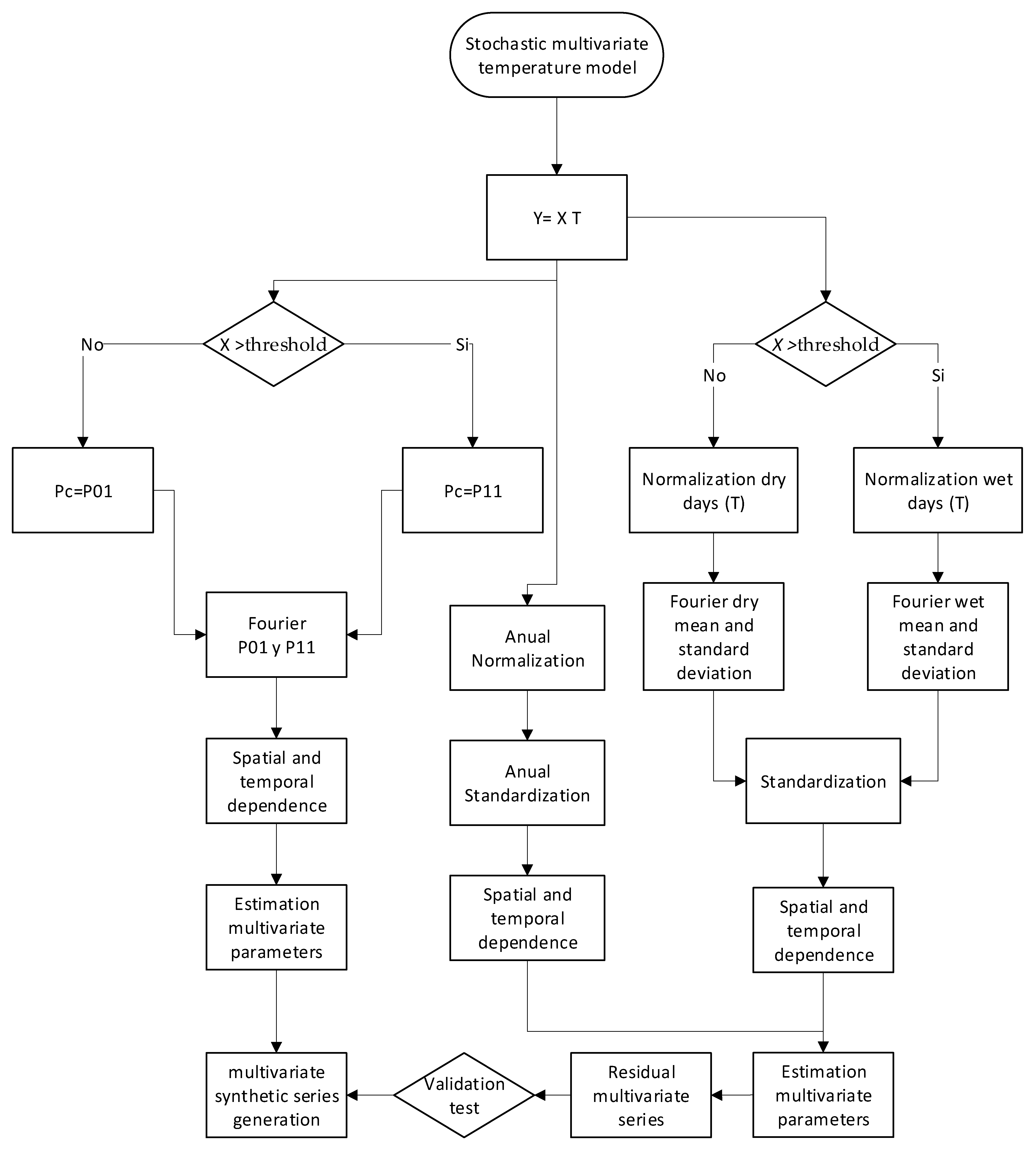
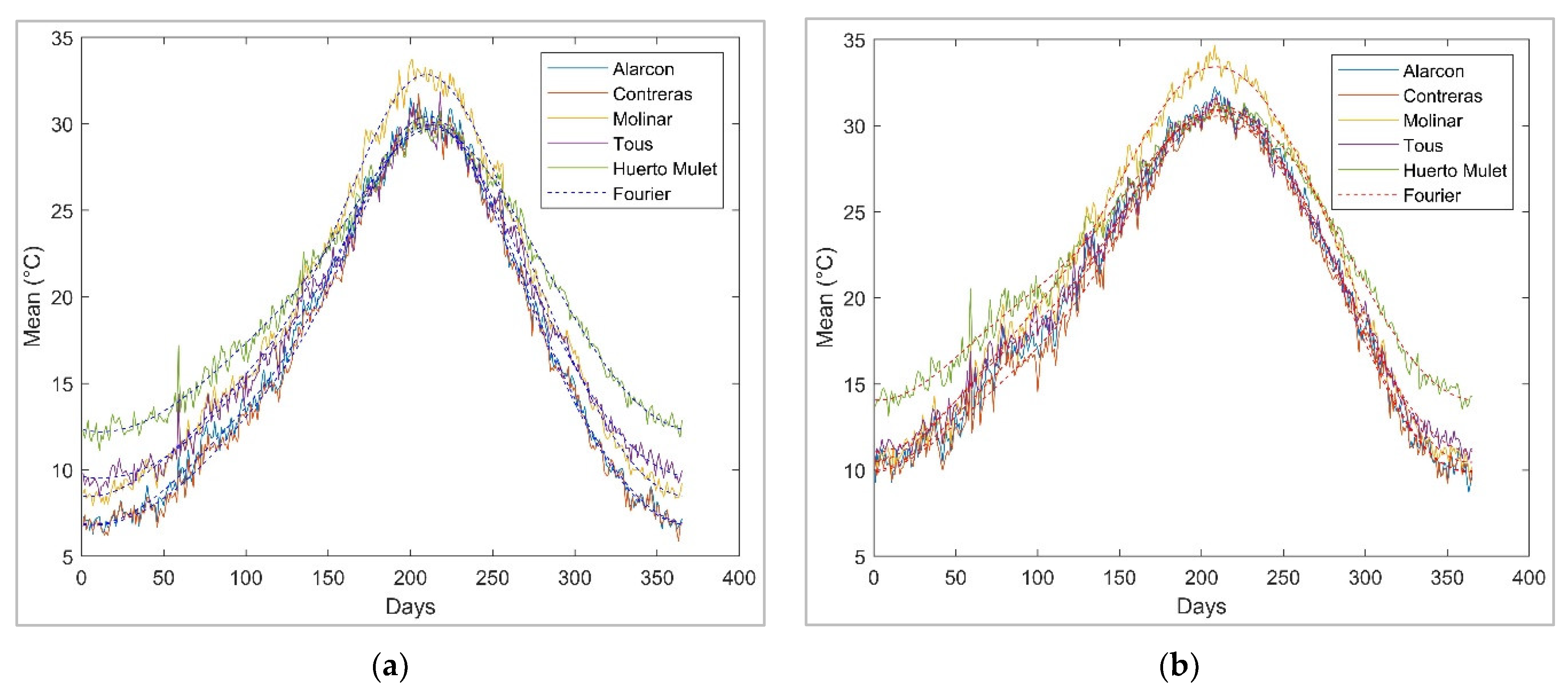
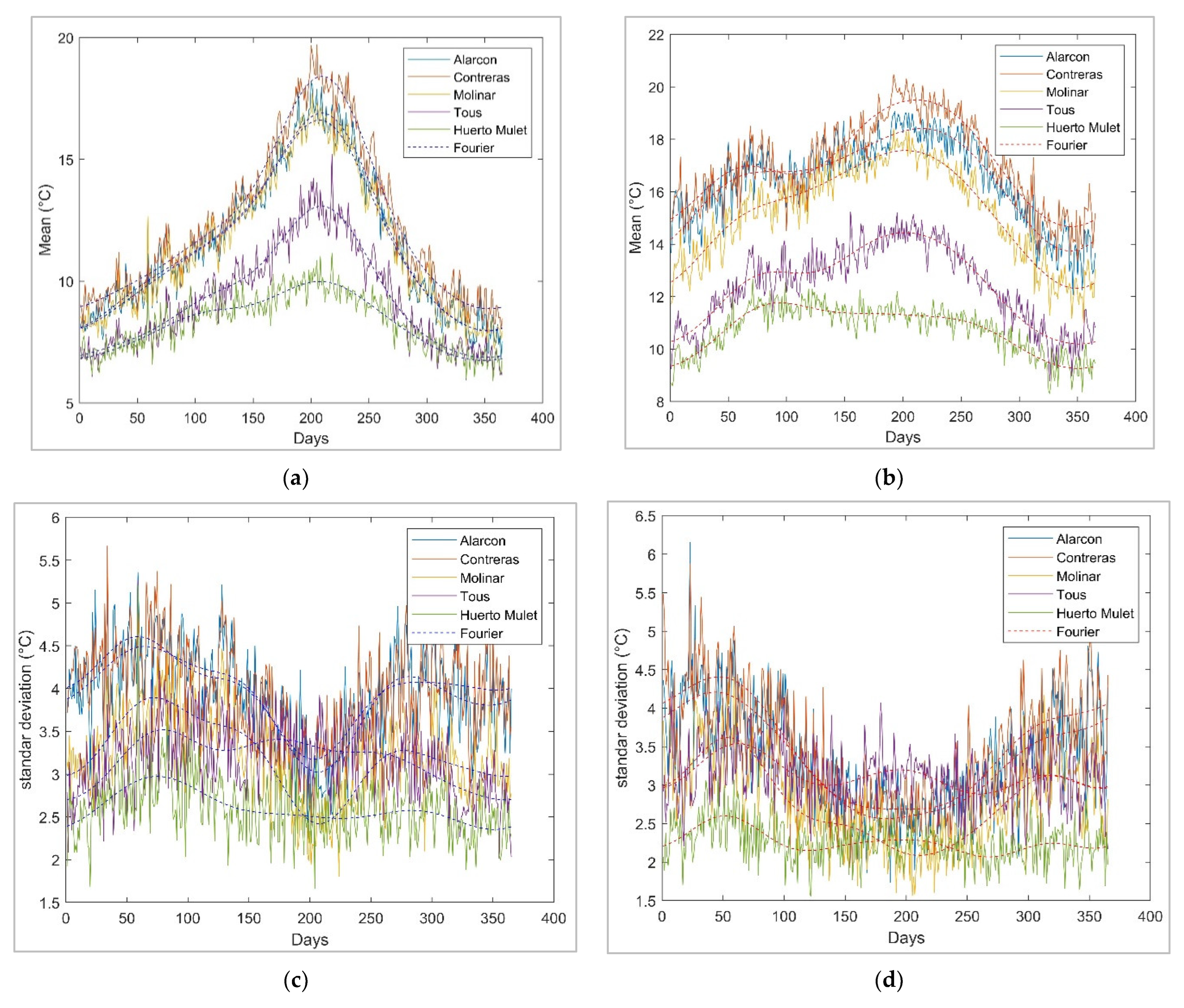
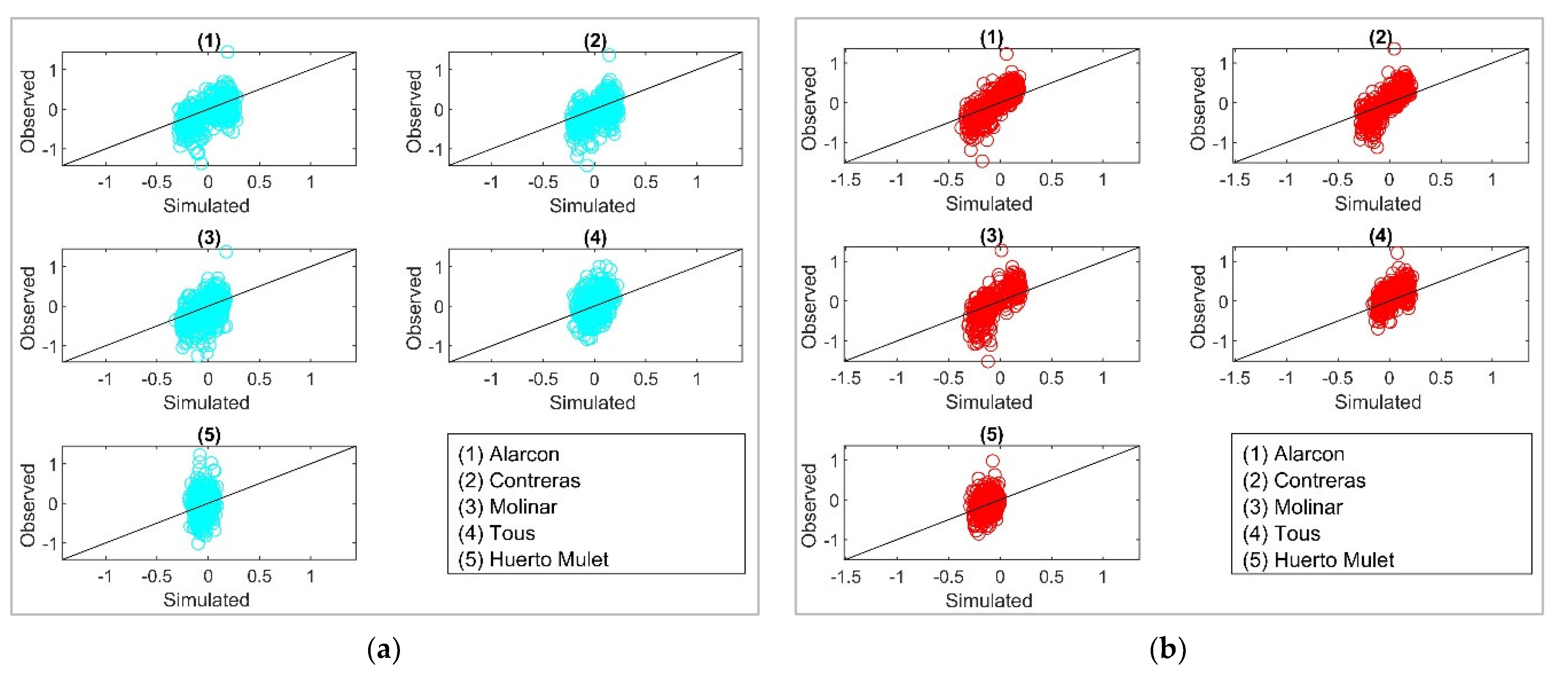
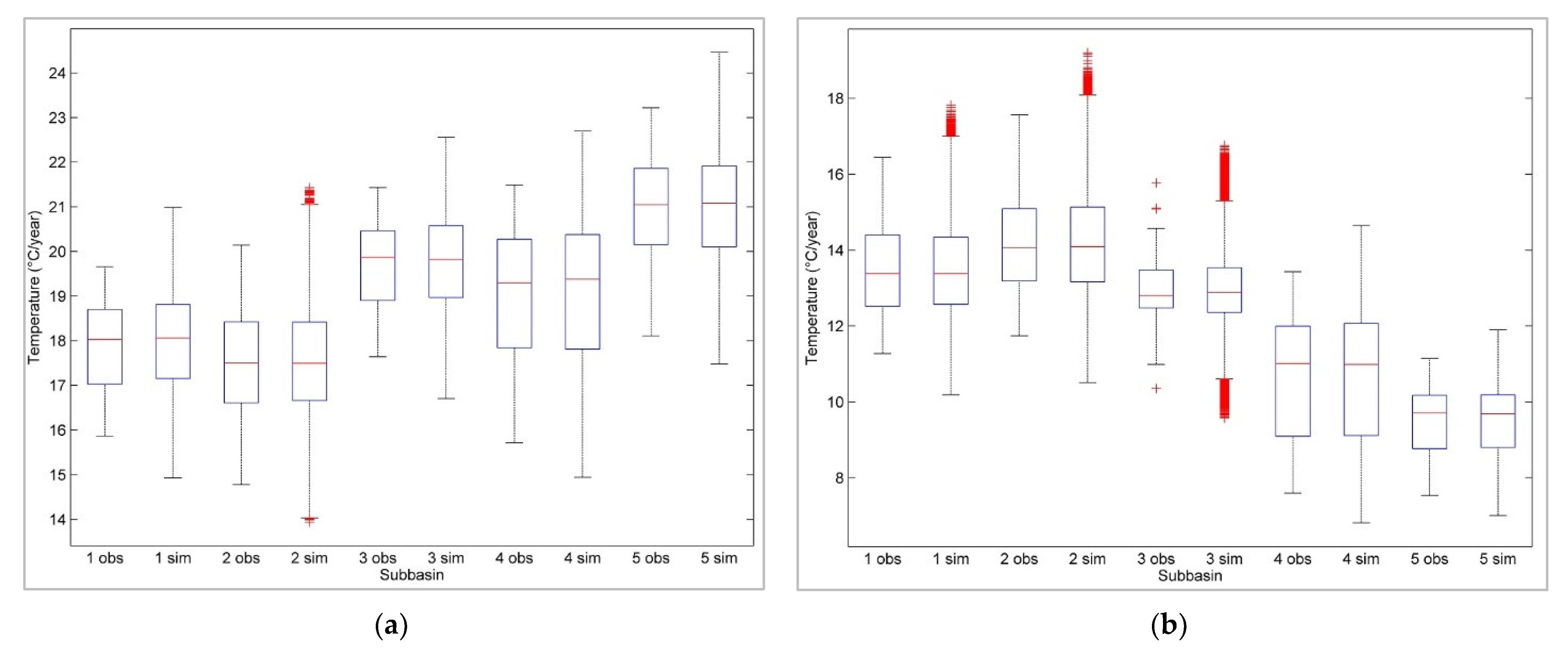
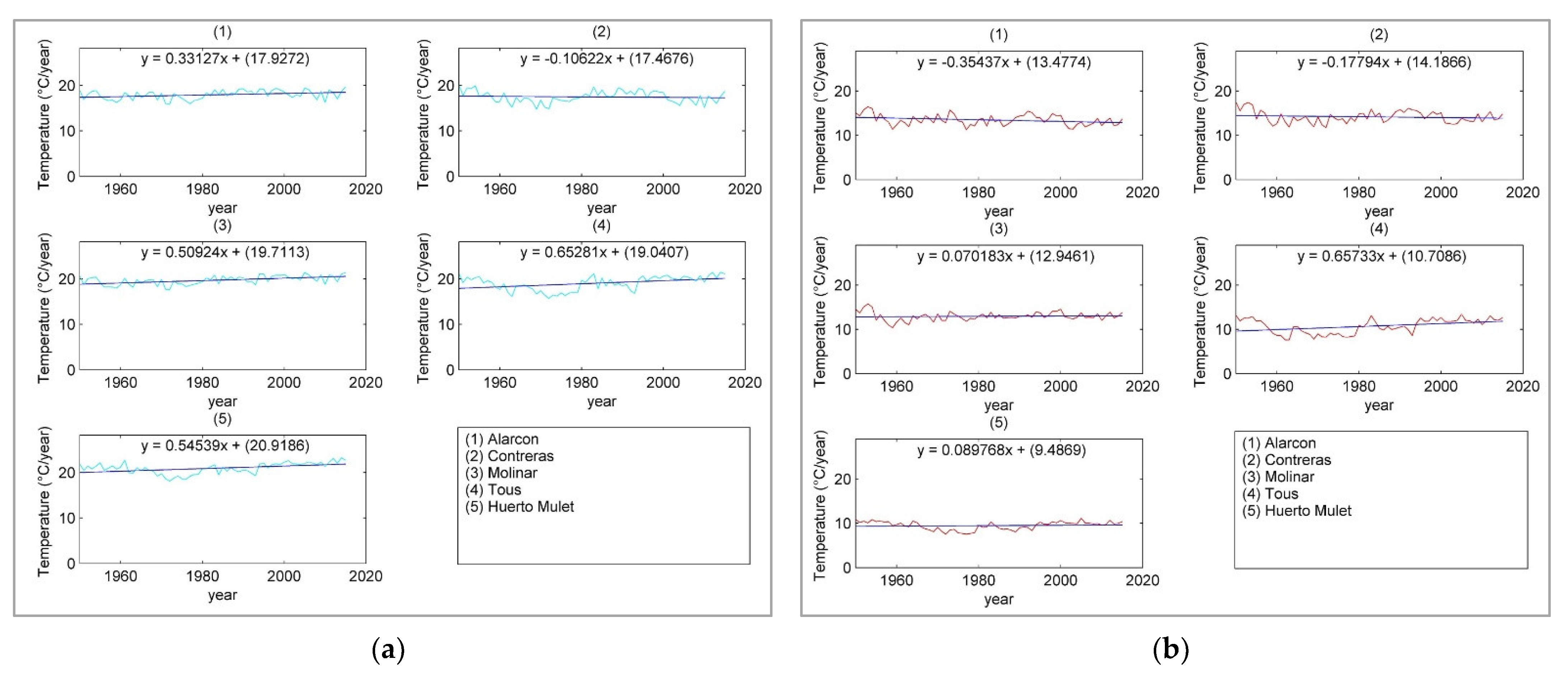
3.2. Stochastic Multisite Multivariate Temperature Series

In the case of the maximum temperature and temperature range, the skewness coefficient of the historical series was near normal. For this reason, we did not consider normalization. Normality was assessed based on the skewness coefficient test for the 95% confidence limit. The daily temperature skewness coefficient was near the normal distribution, according to the confidence limits (Figure 4).
Fourier series was applied to the mean and standard deviation ( μ τ ,   s τ ), and the objective was to reduce the number of parameters (Figure 5). The series were carried out with four parameters, which provide a good fit for the model for the Jucar River Basin. In Figure 5, we can observe the mean, standard deviation, and the Fourier series for the stochastic models for wet and dry days with a 95% confidence interval. The results from fitting Fourier series for the model in Figure 5a,b reflect the smoothed mean for wet and dry days. In case of the standard deviation presented in Figure 6a,b, the fitted curve includes the original data noise.
We calculated the standardization based on the normal series, mean, and standard deviation of the fitted series. The objective of the standardization is to remove the series periodicities and to obtain a mean of zero and variance of one. On the other hand, the standardized series were determined by the multivariate autoregressive model. For the Jucar River Basin, we defined the autoregressive parameters and residual series for different wet thresholds.
We selected the wet threshold of 0.001 for determining the temperature multisite multivariate stochastic generator. First, we evaluated the normality of the residual series. Mean, deviation, skewness coefficient, and lag-one autocorrelation were calculated (Table 1).
The autocorrelation for this series was also determined within the 95% confidence limits for both models’ maximum temperature and temperature range. In addition, we applied different tests to confirm that the residual series can be considered a normal distribution with a mean of zero, variance of one, and skewness coefficient of zero (Figure 7). The residual series of the two developed stochastic models were very similar.
The residual series of the MAR(1) for the maximum temperature had a mean near zero, the variance was around 0.85, the skewness coefficient was between −0.245 and 0.026, and the lag-one autocorrelation was around ± 0.01. The skewness coefficient and autocorrelation are within the confidence limits, the average is within 99% of the confidence limits, and therefore we assumed the normality of the residual series (Table 2).
On the other hand, the series was also considered stationary since it complied with 1 < 1 for all sub-basins. The AIC value was −10,152 with the examined parameters.
Similar results were obtained for the stochastic model for temperature range: the residual series had a mean of around −0.0005, variance of at least 0.92, skewness coefficient between −0.044 and 0.112, and lag-one autocorrelation of about ± 0.08 (Figure A5). For this stochastic model, we assumed normality and stationarity of the residual series as well as for stochastic Model 1 (Table 2). According to the AIC, the stochastic maximum temperature model (M1) was similar to the stochastic temperature range (M2) for all sub-basins.

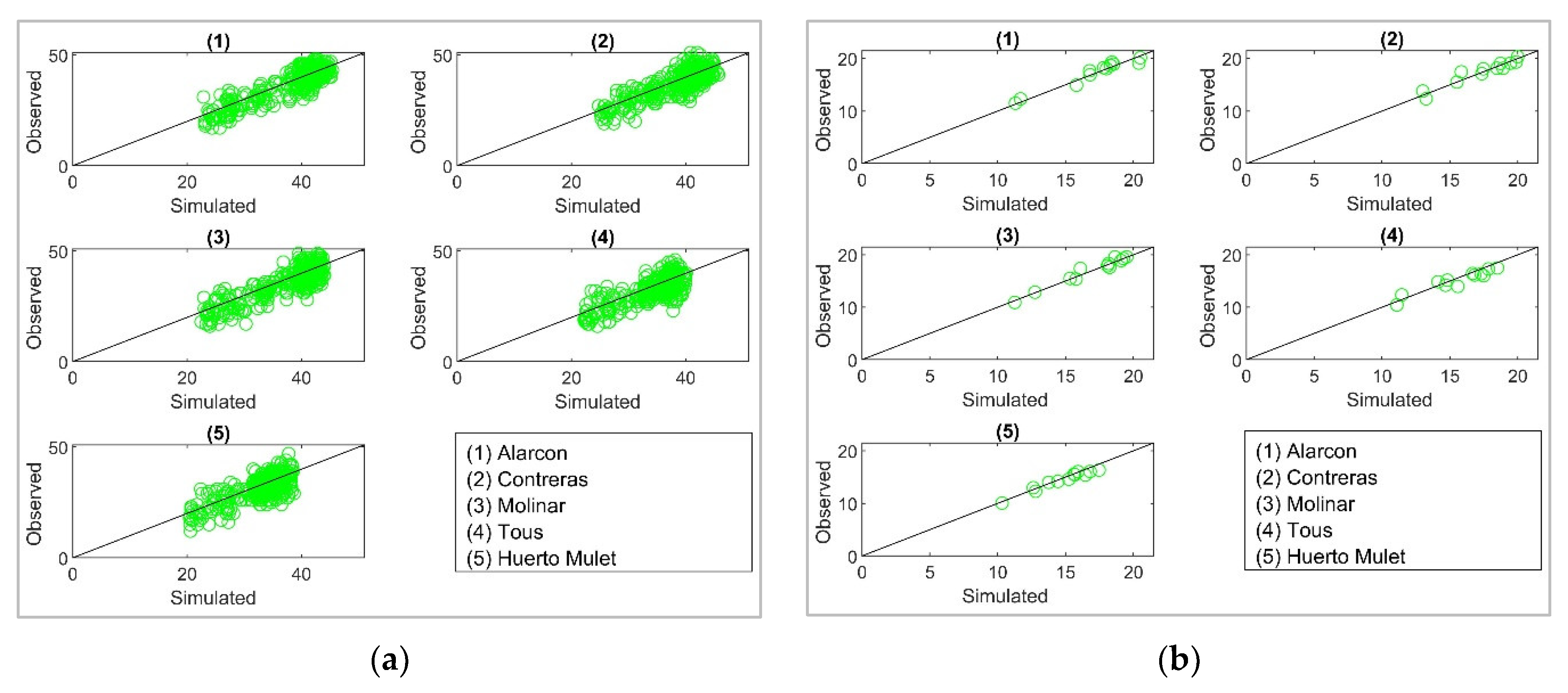
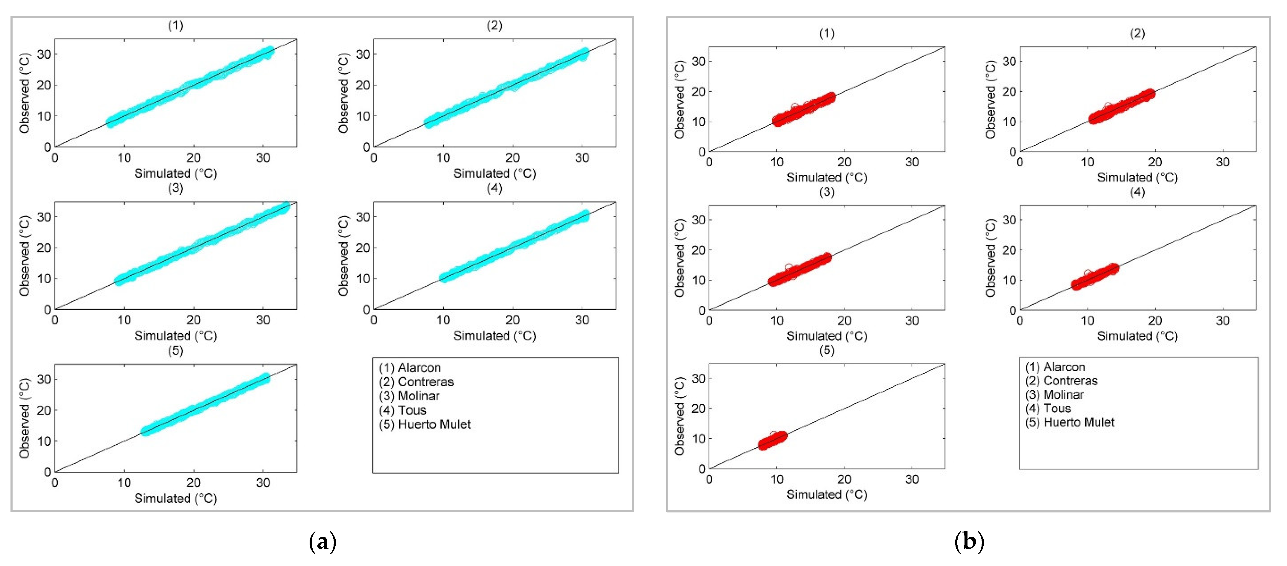
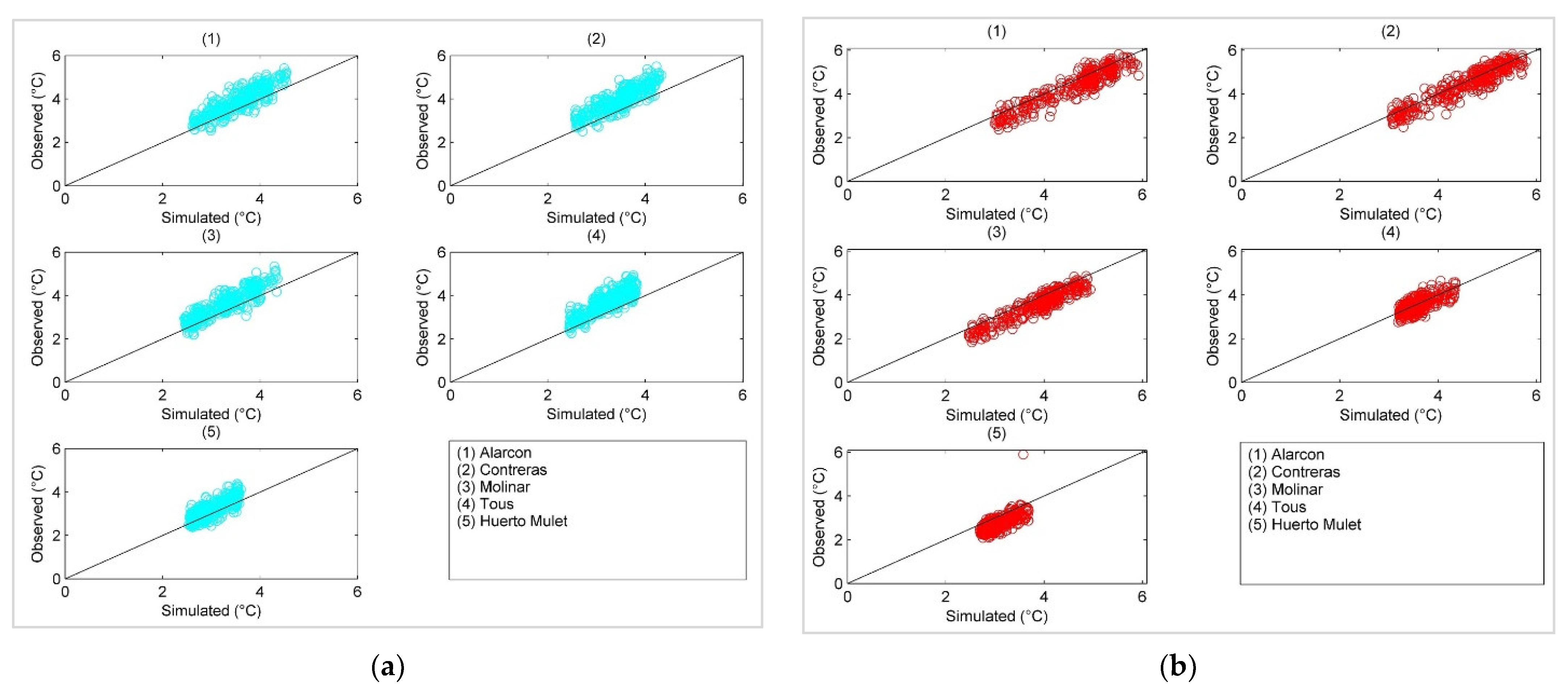
3.3. Generation of Multivariate Synthetic Temperature Series

For the process of generating synthetic series, 1000 series were created considering the same length as the sample (66 years). The statistical sum, mean, standard deviation, and skewness coefficient were determined for both the synthetic and historical series. The occurrence depends on the correlated multivariate precipitation probabilities, critical probability, and normal distribution. Multivariate synthetic series of rainfall occurrences were generated for the five sub-basins using the stochastic process. The same occurrence series was applied for both Model 1 (M1) and Model 2 (M2) to avoid the bias from the MAR(1) model.
For the historical series, the sum of the number of rainy days in 66 years was calculated. In the same way, the monthly occurrences of the synthetic and the historical series were determined. Several statistical tests were performed to validate that the generated series are not substantially different from the historical period. The tests applied to the precipitation occurrence were the k-s test to verify that the results come from the same distribution, the t-test for equality of means, and the Wilcoxon test for equality of medians. The tests were applied considering a 95% reliability, and it was concluded that there is insufficient evidence to refute that the generated precipitation occurrences and historical series, both monthly and daily, are significant.
The scatter plots of daily mean occurrences (66 years) of historical versus simulated data can be seen in Figure 8 for the five sub-basins. The daily rainfall occurrences varied ± 5 days from the 1:1 line (Figure 8a). The monthly rainfall occurrences varied by ± 0.2 days. Monthly occurrences provide better results than daily occurrences due to the number of parameters applied (four in total). We used the same simulated rainfall occurrence (four parameters) to generate the maximum temperature and temperature range.
The statistical mean, standard deviation, and skewness coefficient of daily data were computed. The MAR(1) for mean daily temperatures had a deviation of ±1 °C, which is more accurate than the stochastic Model 2 for the daily average temperature range (±1.5 °C). Model 1 achieved better results on both a daily and a monthly scale (Figure 9). The observed and generated series were not significantly different according to the k-s test, which indicates that they originate from the same distribution, in addition to sharing the same average according to the t-test and the same median according to the Wilcoxon test. These tests were applied to the daily average temperatures and the monthly averages. The best approximations were provided for the monthly data with higher reliability. Moreover, the RMSE, MAE, and PE (Table 3) display the adequate performance of Model 1 (M1) and Model 2 (M2).
The f-test was used for the standard deviation (Figure 10), which indicates the equality of deviations for both models and showed minor differences. Both the maximum temperature and temperature range performed well in the daily standard deviation. It is worth mentioning that the deviations were overestimated concerning the observed data. For a monthly scale, both models effectively reproduced the standard deviation.
Regarding the skewness coefficient, MAR(1) was underestimated for the observed data. The same dispersion was present for the two models (M1 and M2) and for the daily and monthly averages (Figure 11).
Even though the normalization’s function can be adjusted on average for the confidence limits, this offers a variation for the observed skewness. The skewness of observed daily data was between −1.2 and 1.2, and the simulated was between −0.5 and 0.5. Therefore, the multivariate stochastic model underestimated the skewness coefficient by less than −0.5 and more than 0.5. On a monthly scale, the skewness of the simulated precipitation distribution was underestimated similarly to the daily scale.
For monthly temperature, the multisite multivariate model preserved the main statistics. Figure 12 presents all months for the 5 sub-basins and 66 years, in which the temporal and spatial dependence was adequately performed. For maximum temperature, the values were between 5.5 and 35 °C, with variability of ±2 °C (Figure 12a). In the case of temperature range, the values were between 5 and 25 °C with the same variability. For the monthly mean of all sub-basins, the error was only ±0.1 °C.
The multisite multivariate stochastic autoregressive Model 1 was selected to compare temperature years with regard to the observed data. The stochastic model can represent the temporal tendency of the results, providing an adequate indication of the yearly temperatures (Figure 13). Due to the design of the multisite multivariate stochastic model corrected by the annual model, we can simulate low frequency. The interannual variability represents the autocorrelation and cross-correlations of observed data (Table 4). The results indicate that variability was well-reproduced for the stochastic process. Moreover, the maximum and minimum values were performed adequately. For annual temperature, the stochastic model can produce the variability of both temperatures. The variability expressed for the model (sim) was greater than the observed data. Accordingly, the MAR(1) can define the maximum and minimum temperature values.

4. Discussion

The multisite multivariate autoregressive stochastic model (MASCV) was developed using MATLAB and was verified for different stations within the same basin with similar results. A Markov model of two states for the multivariate precipitation occurrence and the conditioned multivariate stochastic model for temperature can represent spatial and temporal parameters to study on-site conditions on daily, monthly, and annual scales. The Markov model of two states with few parameters has been able to depict the precipitation occurrence process. On the other hand, the temperature was accomplished considering normal distribution. Therefore, a reduction of parameters was achieved in generating the temperature. This represents a critical simplification in obtaining the daily temperature, which according to the performed parameterization, provides acceptable results for the Jucar River Basin. Moreover, it simplifies the complexity and reduces computational time.
The stochastic multivariate autoregressive model with few parameters adequately reproduced the daily and monthly temperatures. The tests showed insignificant differences between the observed and generated temperatures.
The primary objective of this stochastic model is to determine the monthly runoff and incorporate it into the integrated water resources management. It is noteworthy that this validation is performed on a monthly scale. Therefore, MASCV must be able to represent the statistics of the precipitation occurrence and temperatures in different timescales. The developed stochastic MAR(1) adequately reproduced the main statistics.

5. Conclusions

The multivariate autoregressive model of climate variables (MASCV) is a daily stochastic weather generator, programmed in MATLAB, with several user advantages, i.e., wet day selection, number of harmonics for each case, normalization type, and synthetic series to generate and automatize graphs. Moreover, MASCV can generate extreme temperatures over extended periods of time. This is unique in stochastic weather generators because only a few can reproduce extreme events. Furthermore, MASVC can be used for bias correction for climate change studies, in this case, perturbing parameters according to climate models. Finally, the results of MASCV can be incorporated for environment analysis.
MASCV presents the completion of a multivariate model for precipitation occurrences, i.e., a Markov model of two states and the dependence of temperature with rainfall occurrence process. This multisite multivariate stochastic model is meant to become a beneficial tool in a simplified manner, which may allow the incorporation of different climatic and hydrological variables.
A Markov model of first order can reflect the time dependence of the precipitation occurrence, preserving comparative statistical data with the historical series. Moreover, the spatial and temporal structure using a stochastic multisite multivariate model and coupling daily and annual temperature correction reproduced adequately in the different timescales.
Models M1 and M2 were suitably performed for different temperatures. For wet and dry days, the multisite multivariate stochastic model can adjust to real dependence with precipitation occurrence and spatial and temporal dependence of daily, monthly, and annual temperatures.
This approach greatly simplifies the process of simulating precipitation, which implies a considerable advantage and versatility over other stochastic generators. The reduction of parameters is an important factor addressed in this approach for determining the temperature and considering continuous modeling for days, months, and years.

Author Contributions

Conceptualization, J.H.-B. and A.S.; methodology, A.S.; software, J.H.-B.; validation, A.S., J.P.-A. and S.T.S.-Q.; formal analysis, A.S.; investigation, J.H.-B.; resources, A.S. and C.D.-S.; data curation, J.H.-B.; writing—original draft preparation, J.H.-B.; writing—review and editing, A.S., J.P.-A., C.D.-S. and S.T.S.-Q.; visualization, A.S.; supervision, J.P.-A.; project administration, A.S. and C.D.-S. All authors have read and agreed to the published version of the manuscript.

Funding

This research received no external funding.

Data Availability Statement

Not applicable.

Acknowledgments

We thank the anonymous reviewers and the editor for their constructive comments on the manuscript.

Conflicts of Interest

The authors declare no conflict of interest.

Appendix A

The spatial and temporal variation of the characteristics of meteorological elements in the Jucar River Basin are presented in Figure A1, Figure A2, Figure A3 and Figure A4, showing the spatial distribution of annual elements based on coordinates and 16 meteorological stations in Jucar River Basin. The grid interpolation uses inverse distance weight interpolation (IDW). Figure A5 shows the daily lag correlation for residual series.
Figure A1. Spatial distribution of annual (a) maximum temperature (°C) and (b) temperature range (°C).
Water 14 03494 g0a1
Figure A2. Spatial distribution of annual (a) precipitation occurrence (wet days/year) and (b) rainfall (mm/year).
Water 14 03494 g0a2
Figure A3. Interannual variation trends of the average (a) maximum temperature (°C) and (b) temperature range (°C).
Water 14 03494 g0a3
Figure A4. Interannual variation trends of the average (a) precipitation occurrence (wet days year−1) and (b) rainfall (mm year−1).
Water 14 03494 g0a4
Figure A5. Daily correlation function for residual series considering the ten lag days: (a) Model 1 (M1) and (b) Model 2 (M2).
Water 14 03494 g0a5

References

  1. Sivakumar, B. Chaos in Hydrology: Bridging Determinism and Stochasticity, 1st ed.; Springer Science: Dordrecht, The Netherlands, 2017; pp. 63–111. [Google Scholar]
  2. Beneyto, C.; Aranda, J.Á.; Benito, G.; Francés, F. New Approach to Estimate Extreme Flooding Using Continuous Synthetic Simulation Supported by Regional Precipitation and Non-Systematic Flood Data. Water 2020, 12, 3174. [Google Scholar] [CrossRef]
  3. Chang, F.; Hsu, K.; Chang, L. Flood Forecasting Using Machine Learning Methods. Water 2019, 2, 14–53. [Google Scholar] [CrossRef] [Green Version]
  4. Chang, F.J.; Guo, S. Advances in Hydrologic Forecasts and Water Resources Management. Water 2020, 12, 1819. [Google Scholar] [CrossRef]
  5. Gabriel, K.R.; Neumann, J. A Markov Chain model for daily rainfall occurrence at tel aviv. Q. J. R. Meteorol. Soc. 1962, 88, 90–95. [Google Scholar] [CrossRef]
  6. Caskey, E. A Markov Chain model for the probability of precipitation occurrence in intervals of various length. Mon. Weather Rev. 1963, 91, 298–301. [Google Scholar] [CrossRef]
  7. Matalas, N.C. Time Series Analysis, 4th ed.; John Wiley & Sons, Inc.: Hoboken, NJ, USA, 1967; Volume 3. [Google Scholar] [CrossRef]
  8. Todorovic, P.; Woolhiser, D.A. A Stochastic Model of n -Day Precipitation. J. Appl. Meteorol. 1975, 14, 17–24. [Google Scholar] [CrossRef]
  9. Richardson, C.W. Stochastic Simulation of Daily Precipitation, Temperature, and Solar Radiation. Water Resour. Res. 1981, 17, 182–190. [Google Scholar] [CrossRef]
  10. Roldán, J. Tendencias Actuales En El Modelado de La Precipitación Diaria. Ing. Agua 1994, I, 89–100. [Google Scholar] [CrossRef] [Green Version]
  11. Rajagopalan, B.; Lall, U.; Tarboton, D.G. Nonhomogeneous Markov Model for Daily Precipitation. J. Hydrol. Eng. 1996, 1, 33–40. [Google Scholar] [CrossRef]
  12. Wilks, D.S. Multisite Generalization of a Daily Stochastic Precipitation Generation Model. J. Hydrol. 1998, 210, 178–191. [Google Scholar] [CrossRef]
  13. Wilks, D.S.S.; Wilby, R.L.L. The Weather Generation Game: A review of stochastic weather models. Prog. Phys. Geogr. 1999, 23, 329–357. [Google Scholar] [CrossRef]
  14. Harrold, T.I. A Nonparametric Model for Stochastic Generation of Daily Rainfall Amounts. Water Resour. Res. 2003, 39, 1–12. [Google Scholar] [CrossRef]
  15. Brissette, F.P.; Khalili, M.; Leconte, R. Efficient Stochastic Generation of Multi-Site Synthetic Precipitation Data. J. Hydrol. 2007, 345, 121–133. [Google Scholar] [CrossRef]
  16. Liu, Y.; Zhang, W.; Shao, Y.; Zhang, K. A comparison of four precipitation distribution models used in daily stochastic models. Adv. Atmos. Sci. 2011, 28, 809–820. [Google Scholar] [CrossRef]
  17. Li, C.; Singh, V.P.; Mishra, A.K. Simulation of the entire range of daily precipitation using a hybrid probability distribution. Water Resour. Res. 2012, 48, 1–17. [Google Scholar] [CrossRef]
  18. Mehrotra, R.; Li, J.; Westra, S.; Sharma, A. A programming tool to generate multi-site daily rainfall using a two-stage semi parametric model. Environ. Model. Softw. 2015, 63, 230–239. [Google Scholar] [CrossRef]
  19. So, B.J.; Kwon, H.H.; Kim, D.; Lee, S.O. Modeling of daily rainfall sequence and extremes based on a semiparametric pareto tail approach at multiple locations. J. Hydrol. 2015, 529, 1442–1450. [Google Scholar] [CrossRef]
  20. Wilks, D.S. Simultaneous stochastic simulation of daily precipitation, temperature and solar radiation at multiple sites in complex terrain. Agric. For. Meteorol. 1999, 96, 85–101. [Google Scholar] [CrossRef]
  21. Semenov, M.A.; Barrow, E.M. LARS-WG A Stochastic Weather Generator for Use in Climate Impact Studies LARS-WG: Stochastic Weather Generator Contents, Harpenden, Hertfordshire, United Kigdom. Available online: http://resources.rothamsted.ac.uk/sites/default/files/groups/mas-models/download/LARS-WG-Manual.pdf (accessed on 10 December 2021).
  22. Chen, J.; Brissette, F.P.; Leconte, R. WeaGETS—A Matlab-Based Daily Scale Weather Generator for Generating Precipitation and Temperature. Procedia Environ. Sci. 2012, 13, 2222–2235. [Google Scholar] [CrossRef]
  23. Salas, J.J.D.; Delleur, J.W.; Yevjevich, V.M.; Lane, W.L. Applied Modeling of Hydrologic Time Series; Water Resources Publication: Littleton, CO, USA, 1980; ISBN 0-918334-37-3. [Google Scholar]
  24. Srikanthan, R.; McMahon, T.A. Stochastic generation of annual, monthly and daily climate data: A review. Hydrol. Earth Syst. Sci. 2001, 5, 653–670. [Google Scholar] [CrossRef] [Green Version]
  25. Qian, B.; Gameda, S.; Hayhoe, H.; De Jong, R.; Bootsma, A. Comparison of LARS-WG and AAFC-WG Stochastic Weather Generators for Diverse Canadian Climates. Clim. Res. 2004, 26, 175–191. [Google Scholar] [CrossRef] [Green Version]
  26. Flecher, C.; Naveau, P.; Allard, D.; Brisson, N. A stochastic daily weather generator for skewed data. Water Resour. Res. 2010, 46, 1–15. [Google Scholar] [CrossRef]
  27. Hayhoe, H.N. Improvements of stochastic weather data generators for diverse climates. Clim. Res. 2000, 14, 75–87. [Google Scholar] [CrossRef]
  28. Ailliot, P.; Allard, D.; Monbet, V.; Naveau, P. Stochastic Weather Generators: An Overview of Weather Type Models. J. Société Française Stat. 2015, 156, 101–113. [Google Scholar]
  29. Richardson, C.W.; Wright, D.A.; Nofziger, D.L.; Hornsby, A.G. WGEN: A Model for Generating Daily Weather Variables. ARS 1984, 8, 1–83. [Google Scholar]
  30. Carter, T.; Posch, M.; Tuomenvirta, H. SILMUSCEN and CLIGEN User’s Guide: Guidelines for the Construction of Climatic Scenarios and Use of a Stochastic Weather Generator in the Finnish. Available online: https://www.osti.gov/etdeweb/biblio/458148 (accessed on 5 November 2021).
  31. Stöckle, C.O.; Nelson, R.; Donatelli, M.; Castellvì, F. ClimGen: A flexible weather generation program. In Proceedings of the 2nd International Symposium Modelling Cropping Systems, Florence, Italy, 17 July 2001. [Google Scholar]
  32. Marcello, D.; Gianni, B.; Ephrem, H.; Simone, B.; Roberto, C.; Bettina, B. CLIMA: A Weather Generator Framework. In Proceedings of the 18th World IMACS/MODSIM Congress, Carins, Australia, 13–17 July 2009; Available online: https://core.ac.uk/download/pdf/38616113.pdf (accessed on 17 July 2009).
  33. Foufoula-georgiou, E.; Lettenmaier, D.P. A Markov renewal model for rainfall occurrences. Water Resour. Res. 1987, 23, 875–884. [Google Scholar] [CrossRef]
  34. Bárdossy, A.; Pegram, G.G.S. Copula Based Multisite Model for Daily Precipitation Simulation. Hydrol. Earth Syst. Sci. 2009, 13, 2299–2314. [Google Scholar] [CrossRef] [Green Version]
  35. Sansom, J. A Hidden Markov Model for Rainfall Using Breakpoint Data. J. Clim. 1998, 11, 42–53. [Google Scholar] [CrossRef]
  36. Ailliot, P.; Thompson, C.; Thomson, P. Space-Time Modelling of Precipitation by Using a Hidden Markov Model and Censored Gaussian Distributions. J. R. Stat. Soc. Ser. C Appl. Stat. 2009, 58, 405–426. [Google Scholar] [CrossRef]
  37. Racsko, P.; Szeidl, L.; Semenov, M. A serial approach to local stochastic weather models. Ecol. Model. 1991, 57, 27–41. [Google Scholar] [CrossRef]
  38. Zheng, X.; Katz, R.W. Mixture Model of Generalized Chain-Dependent Processes and Its Application to Simulation of Interannual Variability of Daily Rainfall. J. Hydrol. 2008, 349, 191–199. [Google Scholar] [CrossRef]
  39. Hannachi, A. Intermittency, Autoregression and Censoring: A First-Order AR Model for Daily Precipitation. Meteorol. Appl. 2014, 21, 384–397. [Google Scholar] [CrossRef]
  40. Khan, R.S.; Abul, M.; Bhuiyan, E.; Khan, R.S.; Bhuiyan, M.A.E.; García-Ortega, E.; Rigo, T. Artificial Intelligence-Based Techniques for Rainfall Estimation Integrating Multisource Precipitation Datasets. Atmosphere 2021, 12, 1239. [Google Scholar] [CrossRef]
  41. Chiang, Y.M.; Chang, F.J.; Jou, B.J.D.; Lin, P.F. Dynamic ANN for Precipitation Estimation and Forecasting from Radar Observations. J. Hydrol. 2007, 334, 250–261. [Google Scholar] [CrossRef]
  42. Cachim, P. ANN Prediction of Fire Temperature in Timber. J. Struct. Fire Eng. 2019, 10, 233–244. [Google Scholar] [CrossRef]
  43. Li, X.; Li, Z.; Huang, W.; Zhou, P. Performance of Statistical and Machine Learning Ensembles for Daily Temperature Downscaling. Theor. Appl. Climatol. 2020, 140, 571–588. [Google Scholar] [CrossRef]
  44. Bochenek, B.; Ustrnul, Z. Machine Learning in Weather Prediction and Climate Analyses—Applications and Perspectives. Atmosphere 2022, 13, 180. [Google Scholar] [CrossRef]
  45. Oses, N.; Azpiroz, I.; Marchi, S.; Guidotti, D.; Quartulli, M.; Olaizola, I.G. Analysis of Copernicus’ Era5 Climate Reanalysis Data as a Replacement for Weather Station Temperature Measurements in Machine Learning Models for Olive Phenology Phase Prediction. Sensors 2020, 20, 6381. [Google Scholar] [CrossRef]
  46. Hernández-Bedolla, J.; Solera, A.; Paredes-Arquiola, J.; Pedro-Monzonís, M.; Andreu, J.; Sánchez-Quispe, S. The Assessment of Sustainability Indexes and Climate Change Impacts on Integrated Water Resource Management. Water 2017, 9, 213. [Google Scholar] [CrossRef] [Green Version]
  47. Tang, Y.; Zeng, G.; Yang, X.; Iyakaremye, V.; Li, Z. Intraseasonal Oscillation of Summer Extreme High Temperature in Northeast China and Associated Atmospheric Circulation Anomalies. Atmosphere 2022, 13, 387. [Google Scholar] [CrossRef]
  48. Yang, Q. Extended-Range Forecast for the Low-Frequency Oscillation of Temperature and Low-Temperature Weather over the Lower Reaches of the Yangtze River in Winter. Chin. J. Atmos. Sci. 2021, 45, 21–36. [Google Scholar] [CrossRef]
  49. Chen, J.; Brissette, F.P.; Leconte, R. A Daily Stochastic Weather Generator for Preserving Low-Frequency of Climate Variability. J. Hydrol. 2010, 388, 480–490. [Google Scholar] [CrossRef]
  50. Hansen, J.W.; Mavromatis, T. Correcting Low-Frequency Variability Bias in Stochastic Weather Generators. Agric. For. Meteorol. 2001, 109, 297–310. [Google Scholar] [CrossRef]
  51. Chen, J.; Arsenault, R.; Brissette, F.P.; Côté, P.; Su, T. Coupling Annual, Monthly and Daily Weather Generators to Simulate Multisite and Multivariate Climate Variables with Low—Frequency Variability for Hydrological Modelling. Clim. Dyn. 2019, 53, 3841–3860. [Google Scholar] [CrossRef]
  52. Apipattanavis, S.; Podestá, G.; Rajagopalan, B.; Katz, R.W. A Semiparametric Multivariate and Multisite Weather Generator. Water Resour. Res. 2007, 43, W11401. [Google Scholar] [CrossRef]
  53. Li, X.; Babovic, V. A New Scheme for Multivariate, Multisite Weather Generator with Inter-Variable, Inter-Site Dependence and Inter-Annual Variability Based on Empirical Copula Approach. Clim. Dyn. 2019, 52, 2247–2267. [Google Scholar] [CrossRef]
  54. Ghosh Dastidar, A.; Ghosh, D.; Dasgupta, S.; De, U.K. Higher Order Markov Chain Models for Monsoon Rainfall over West Bengal, India. Indian J. Radio Space Phys. 2010, 39, 39–44. [Google Scholar]
  55. Hosseini, R.; Le, N.; Zidek, J. Selecting a Binary Markov Model for a Precipitation Process. Environ. Ecol. Stat. 2011, 18, 795–820. [Google Scholar] [CrossRef]
  56. Lennartsson, J.; Baxevani, A.; Chen, D. Modelling Precipitation in Sweden Using Multiple Step Markov Chains and a Composite Model. J. Hydrol. 2008, 363, 42–59. [Google Scholar] [CrossRef] [Green Version]
  57. Otienoongála, J.; Ster, D.; Stern, R. Extending Genstat Capability to Analyze Rainfall Data Using a Markov Chain Model. Eur. Sci. J. August Ed. 2012, 8, 1857–7881. [Google Scholar]
  58. Chen, J.; Brissette, F.P. Stochastic Generation of Daily Precipitation Amounts: Review and Evaluation of Different Models. Clim. Res. 2014, 59, 189–206. [Google Scholar] [CrossRef] [Green Version]
  59. Woolhiser, D.A.; Pegram, G.G.S. Maximum Likelihood Estimation of Fourier Coefficients to Describe Seasonal Variations of Parameters in Stochastic Daily Precipitation Models. J. Appl. Meteorol. 1979, 18, 34–42. [Google Scholar] [CrossRef]
  60. Keller, D.E.; Fischer, A.M.; Frei, C.; Liniger, M.A.; Appenzeller, C.; Knutti, R. Implementation and Validation of a Wilks-Type Multi-Site Daily Precipitation Generator over a Typical Alpine River Catchment. Hydrol. Earth Syst. Sci. 2015, 19, 2163–2177. [Google Scholar] [CrossRef]
  61. Chen, J.; Brissette, F.P. Comparison of Five Stochastic Weather Generators in Simulating Daily Precipitation and Temperature for the Loess Plateau of China. Int. J. Climatol. 2014, 34, 3089–3105. [Google Scholar] [CrossRef]
  62. Sakia, R.M. The Box-Cox Transformation Technique: A review. J. R. Stat. Soc. 1992, 41, 169–178. [Google Scholar] [CrossRef]
  63. Anderson, R.L. Distribution of the Serial Correlation Coefficient. Ann. Math. Stat. 1942, 13, 1–13. [Google Scholar] [CrossRef]
  64. Moors, D. Stubblebine Chi-Square Tests for multivariate normality with application to common Stock prices. Comun. Stat. -Theory Methods 1981, 10, 713–738. [Google Scholar] [CrossRef]
  65. Hu, S. Akaike Information Criterion Statistics. Math. Comput. Simul. 1987, 29, 452. [Google Scholar] [CrossRef]
  66. Pedro-Monzonís, M.; Ferrer, J.; Solera, A.; Estrela, T.; Paredes-Arquiola, J. Key Issues for Determining the Exploitable Water Resources in a Mediterranean River Basin. Sci. Total Environ. 2015, 503–504, 319–328. [Google Scholar] [CrossRef] [Green Version]
  67. Pérez-Martín, M.A.; Thurston, W.; Estrela, T.; del Amo, P. Cambio En Las Series Hidrológicas de Los Últimos 30 Años y Sus Causas. El Efecto 80. III Jorn. Ing. Agua (JIA 2013). La Protección Contra Los Riesgos Hídricos 2013, 2, 527–534. [Google Scholar]
  68. CHJ Plan Hidrológico de La Demarcación Hidrográfica Del Júcar, Memoria-Anejo 2. CJH, Valencia, España. 2015. Available online: https://www.chj.es/es-es/medioambiente/planificacionhidrologica/Paginas/PHC-2015-2021-Plan-Hidrologico-cuenca.aspx (accessed on 10 December 2021).
  69. Herrera, S.; Fernández, J.; Gutiérrez, J.M. Update of the Spain02 Gridded Observational Dataset for EURO-CORDEX Evaluation: Assessing the Effect of the Interpolation Methodology. Int. J. Climatol. 2016, 36, 900–908. [Google Scholar] [CrossRef] [Green Version]
  70. Daly, C. Guidelines for Assessing the Suitability of Spatial Climate Data Sets. Int. J. Climatol. 2006, 26, 707–721. [Google Scholar] [CrossRef]
  71. Pérez-Martín, M.A.; Estrela, T.; Andreu, J.; Ferrer, J.; Pérez-Martín, M.A.; Andreu, J.; Estrela, T.; Ferrer, J. Modeling Water Resources and River-Aquifer Interaction in the Júcar River Basin, Spain. Water Resour. Manag. 2014, 28, 4337–4358. [Google Scholar] [CrossRef]
  72. Melsen, L.; Teuling, A.; Torfs, P.; Zappa, M.; Mizukami, N.; Clark, M.; Uijlenhoet, R. Representation of Spatial and Temporal Variability in Large-Domain Hydrological Models: Case Study for a Mesoscale Pre-Alpine Basin. Hydrol. Earth Syst. Sci. 2016, 20, 2207–2226. [Google Scholar] [CrossRef]
  73. Parlange, M.B.; Katz, R.W.; Parlange, M.B.; Katz, R.W. An Extended Version of the Richardson Model for Simulating Daily Weather Variables. J. Appl. Meteorol. 2000, 39, 610–622. [Google Scholar] [CrossRef]
Figure 1. Proposed methodology for multisite multivariate precipitation occurrence, daily and annual temperatures.
Water 14 03494 g001
Figure 2. Location of Jucar River Basin.
Water 14 03494 g002
Figure 3. Fourier series and confidence limits for Alarcon: (a) p 01 (b) p 11 with four parameters. Confidence limits at 95% (lower and upper limits).
Water 14 03494 g003
Figure 4. Skewness coefficient (daily average) of normalized series (66 years): (a) maximum temperature and (b) temperature range. Anderson confidence limits (95%).
Water 14 03494 g004
Figure 5. Fourier series (daily average) of maximum temperature series (66 years): (a) mean wet days, (b) mean dry days, (c) standard deviation wet days, and (d) standard deviation dry days.
Water 14 03494 g005aWater 14 03494 g005b
Figure 6. Fourier series (daily average) of temperature range series (66 years): (a) mean wet days, (b) mean dry days, (c) standard deviation wet days, and (d) standard deviation dry days.
Water 14 03494 g006
Figure 7. Theoretical normal distribution (blue) and histogram for residual series for all sub-basins: (a) Model 1 (maximum temperature) and (b) Model 2 (temperature range).
Water 14 03494 g007
Figure 8. Scatter plots for rainfall occurrence (mean 66 years observed and 1000 simulated series) for the five sub-basins: (a) daily mean for each calendar day (green) and (b) monthly mean for each calendar moth (green) for M1 and M2.
Water 14 03494 g008
Figure 9. Scatter plots for observed mean versus generated temperature (mean 66 years observed and 1000 simulated series) for two models: (a) maximum temperature for each calendar day (blue) and (b) temperature range for each calendar day (red).
Water 14 03494 g009
Figure 10. Scatter plots for observed standard deviations versus generated (mean 66 years observed and 1000 simulated series) for two models: (a) maximum temperature for each calendar day (blue) and (b) temperature range for each calendar day (red).
Water 14 03494 g010
Figure 11. Scatter plots for observed skewness coefficient versus generated (mean 66 years observed and 1000 simulated series) for two models: (a) maximum temperature for each calendar day (blue) and (b) temperature range for each calendar day (red).
Water 14 03494 g011
Figure 12. Monthly temperature for all sub-basins (mean 66 years observed and 1000 simulated series) observed and simulated for (a) maximum temperature for each month (blue) and (b) temperature range for each month (red), for 66 years, 5 sub-basins, and all months.
Water 14 03494 g012
Figure 13. Yearly temperature for all sub-basins observed (obs) and simulated (sim) for (a) maximum temperature and (b) temperature range. (1) Alarcon, (2) Contreras, (3) Molinar, (4) Tous, and (5) Huerto Mulet. The outliers are plotted individually using the ‘+’ marker symbol.
Water 14 03494 g013
Table 1. AIC for different wet thresholds and stochastic occurrence model.
Sub-BasinWet Day Threshold (mm)
0.001 *0.010.100.25
Alarcon−590.2−515.3−362.2−310.9
Contreras−681.5−551.2−459.5−421.3
Molinar−562.3−420.7−261.2−215.1
Tous−587.4−463.6−380.5−340.0
Huerto Mulet−610.5−554.7−467.3−427.3
* Best performance.
Table 2. Normality analysis for residual series for M1 and M2 (wet threshold 0.001).
ModelStatistical/Sub-BasinAlarconContrerasMolinarTousHuerto Mulet
1 *Mean−6.7 × 10⁻⁵−2.0 × 10−47.5 × 10−5−2.6 × 10−45.6 × 10−5
Deviation0.8420.8210.8340.8120.850
Skewness coefficient−0.185−0.242−0.245−0.0890.026
Lag-one autocorrelation 0.0050.0030.009−0.041−0.042
AIC−8369−9508−8814−10,152−7958
2 **Mean−3.09 × 10⁻⁴−5.98 × 10⁻⁴−6.83 × 10⁻⁵−2.70 × 10⁻⁴−2.65 × 10⁻⁴
Deviation0.9370.9200.9420.9000.942
Skewness coefficient−0.009−0.038−0.0440.112−0.028
Lag-one autocorrelation 0.0360.043−0.030−0.082−0.039
AIC−6471−8233−5957−10,294−5896
* Maximum temperature. ** Temperature range.
Table 3. Performance analysis for Model 1 and Model 2.
ParameterModel 1 (M1)Model 2 (M2)
1234512345
RMSE (°C/day)1.8811.1071.3921.1560.7671.7861.0191.2901.0780.780
MAE (°C/day)1.5030.8201.0920.8960.5721.4550.7731.0210.8520.582
PE (%)0.0430.0270.0170.0310.0210.0350.0490.0400.0250.012
Table 4. Annual cross-correlation matrix for all sub-basins.
Maximum Temperature Cross-Correlation
Sub-BasinAlarconContrerasMolinarTousHuerto M* Alarcon* Contreras* Molinar* Tous* Huerto M
Alarcon1.000 1.000
Contreras0.8331.000 0.8341.000
Molinar0.7600.7971.000 0.7650.8191.000
Tous0.2390.4920.5981.000 0.2430.4890.6101.000
Huerto M0.2230.3710.3900.8021.0000.2300.3770.3980.8001.000
Temperature Range Cross-Correlation
Sub-BasinAlarconContrerasMolinarTousHuerto M* Alarcon* Contreras* Molinar* Tous* Huerto M
Alarcon1.000 1.000
Contreras0.7191.000 0.7181.000
Molinar0.8910.5921.000 0.8950.5901.000
Tous0.5630.4940.7541.000 0.5650.4990.7591.000
Huerto M0.5040.3310.7100.9181.0000.5020.3330.7080.9171.000
* Simulated cross-correlation.
Publisher’s Note: MDPI stays neutral with regard to jurisdictional claims in published maps and institutional affiliations.

