
Estimation of Latent Heat Flux Using a Non-Parametric Method


1
Department of Bioenvironmental Systems Engineering, National Taiwan University, Taipei 10617, Taiwan
2
Civil and Environmental Engineering Department, Environmental Research Institute, University College Cork, Cork T12P2FY, Ireland
*
Author to whom correspondence should be addressed.
Water 2022, 14(21), 3474; https://doi.org/10.3390/w14213474
Submission received: 29 September 2022
/
Revised: 22 October 2022
/
Accepted: 27 October 2022
/
Published: 30 October 2022
(This article belongs to the Section Hydrology)
Abstract
:The non-parametric (N-P) method expresses evapotranspiration as a function of net radiation, ground heat flux, air temperature, and surface temperature (Ts). This method is relatively new and attractive for estimating evapotranspiration, especially for Ts measurements from remote sensing. The purpose of this study is to investigate the limitations of this method and compare its performance with those of the Penman–Monteith (P–M) and Priestley–Taylor (P–T) equations. Field experiments were carried out to study the evapotranspiration rates and sensible heat fluxes above three different ecosystems: grassland, peat bog, and forest. The results show that above the grassland and peat bog, the evapotranspiration rates were close to the equilibrium evaporation. Though the forest is humid (average humidity ≈ 89%; annual precipitation ≈ 2600 mm), the evapotranspiration was only 69% of the equilibrium evaporation. In terms of model predictions, it was found that the P–M and P–T equations were able to predict the water vapor and sensible heat fluxes well (R2 ≈ 0.60–0.92; RMSE ≈ 30 W m−2) for all the three sites if the canopy resistance and the P–T constant of the ecosystem were given a priori. However, the N-P method only succeeded for the grassland and peat bog; it failed above the forest site (RMSE ≈ 60 W m−2). Our analyses and field measurements demonstrated that for the N-P method to be applicable, the actual evapotranspiration of the site should be within 0.89–1.05 times the equilibrium evaporation.
1. Introduction
Evapotranspiration (water vapor flux) is an important component of the water cycle, surface energy balance, and water resources. In order to accurately estimate water vapor fluxes, many methods have been developed [1,2]. Among them, the Penman–Monteith (P–M) equation [3] is the most widely used. However, the parameter in the P–M equation, canopy resistance, is needed a priori. Hence, the inconvenience and uncertainty of applying the P–M equation are having to parameterize the canopy resistance using primary meteorological data [4,5,6].
Priestley and Taylor proposed a simplified method, the Priestley–Taylor (P–T) equation, which mainly incorporates the effects of the unsaturated atmospheric demand term in the P–M equation into a single empirical constant [7,8]. Nevertheless, calibration for the empirical constant (Priestley and Taylor constant) is also necessary for successfully implementing the P–T equation [4,9,10].
To avoid the uncertainty caused by parameterization of canopy resistance in the P–M equation, Liu et al. [1] proposed a non-parametric (N-P) method based on Hamilton’s principle [11] to estimate fluxes of water vapor (LE) and sensible heat (H). This method does not require empirical parameters, and directly uses the measured meteorological data as model inputs (i.e., net radiation, air temperature, ground heat flux, and surface temperature) to estimate surface fluxes. In their study, Liu et al. evaluated this method at 26 sites and found that 23 sites performed well, and even when compared to the P–M equation and Bowen ratio method, the non-parametric method was found to perform best [1]. This method is particularly attractive for estimating LE with remote sensing data [12,13,14,15]. However, this method has not yet been tested over tall canopies (e.g., forests).
Yang et al. [16] evaluated the non-parametric method over two corn croplands and one bare soil site. They concluded that this method would overestimate water vapor flux under dry conditions and that use the non-parametric method in a dry environment should be avoided. Adopting this non-parametric method and using satellite data from a Moderate-Resolution Imaging Spectroradiometer (MODIS) and the China Meteorological Administration Land Data Assimilation System, Pan et al. [14] retrieved LE over an arid region and found that the LE was underestimated at all four sites. In addition, Pan et al. [12,13] showed that the non-parametric approach performed better above humid areas (e.g., wetland, vegetable site).
In summary, the non-parametric method is found to be unsuitable for arid environments but is still attractive for humid regions. Studies evaluating this method over humid conditions are still rare, especially for tall canopy environments (e.g., forests). The purpose of this study is to examine the non-parametric method above three different humid areas (grassland, peat bog, and montane forest) for estimating LE and H and compare its performance with two traditional methods: the P–M and P–T equations.
2. Experiments
Field experiments conducted over the three humid sites: grassland, peat bog, and montane forest, are described below.
2.1. Grassland
The grassland site is located approximately 25 km northwest of Cork in southern Ireland (59°59′ N, 8°45′ W; 195 m above sea level). This area has a rainy temperate climate with an annual average temperature of 9.4 °C and rainfall of 1207 mm. The annual average temperature during this study period (1 January 2013–31 December 2013) was 9 °C, mean humidity was 92%, and the annual rainfall was 1161 mm. This grassland site is a high-quality pasture and grassland, with perennial ryegrass as the main plant species, mixed with a small amount of foxtail grass and fluffy grass. Grass height was about 10–20 cm in pastures and up to 45 cm in grassland [17]. The average canopy height was 30 cm in year 2013. The soil type is gley with fertile soil, and the proportion of soil particle size is 42% sand, 41% silt, and 17% clay [18]. Soil organic carbon concentration was 5.9% in a 20 cm deep soil layer [19]. An eddy covariance (EC) system, which consisted of a CO2/H2O gas analyzer (Li-7500) and an ultrasonic anemometer (CSAT), was installed at 5 m above the ground. The sampling frequency and averaging period for this system were 10 Hz and 30 min, respectively.
Other measured meteorological data include net radiation (Rn), ground heat flux (G), air temperature (Ta), surface temperature (Ts), and relative humidity (RH). Soil thermometers were set up at 1.5, 5, and 7.5 cm below the ground, respectively. The measured frequency was one datum per minute, and the data was then averaged every 30 min. The site description and instrumentation are also summarized in Table 1. Additional experimental details can be found in Peichl et al. [20].
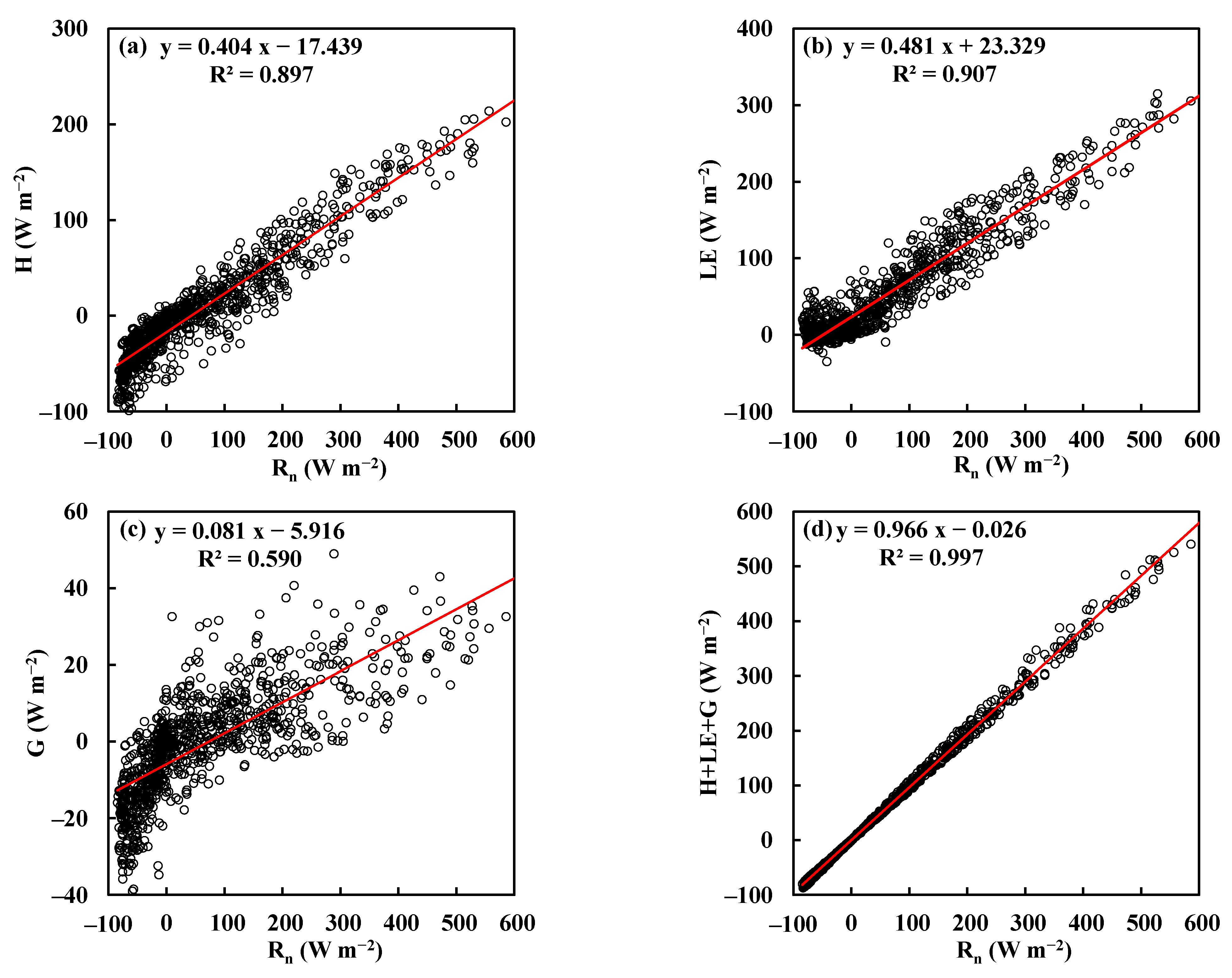
All of the three methods (P–M equation, P–T equation, N-P method) for estimating LE assume that the surface energy is closed (i.e., Rn = H+LE+G). For the purpose of this study, only data that satisfy the energy closure condition within 90% were selected. In other words, the difference between Rn and H+LE+G should be within ±10%. This data selection process was also applied to the other two sites (peat bog and forest). Figure 1 shows the scatter plots between Rn and H, LE, G, and H+LE+G. From Figure 1, we notice that in this grassland site, about 40% of the energy was used for warming the air (Figure 1a); 48% was distributed to evapotranspiration (Figure 1b); less than 10% of the energy was transported to the ground (Figure 1d); and the overall energy closure rate was about 97% after data selection using the energy closure condition. These energy partition coefficients are also summarized in Table 2.
2.2. Peat Bog
The peat bog site is an Atlantic blanket bog located at Glencar, County Kerry, south-west Ireland (51°55′ N, 9°55′ W, 150 m above sea level). This area also has a rainy temperate climate, with an average temperature of 10.1 °C, an average humidity of around 82%, and an annual rainfall of 1834 mm during the experimental period. In the center of the bog, the peat layer in the upper half consists mainly of reed sedge peat; the bulk density of the soil is 0.05 (g cm−3), the porosity is 95%, and the depth of the peat layer varies from about 2 to 5 m [21]. In the southern part of the bog, there is a drainage river with a catchment area of 74 ha, of which about 85% of the surface is blanket peat, and the other 15% is grazing grassland and drained peat soils.
According to relative elevation, the landform of this site can be divided into four categories: hummocks (6%), high lawns (62%), low lawns (21%), and hollows (11%) [22]. Vascular plants and Bryophytes cover about 30% and 25% of the surface, respectively, in summers. The main species here are Racomitrium lanuginosum (Hedw.) Brid. and bog moss, in roughly equal proportions [23]. The average canopy height here was about 10 cm.
To measure fluxes of sensible heat, water vapor, and carbon dioxide, an eddy covariance system was installed at 3 m above the ground in the center of the peat bog. This EC system consisted of an ultrasonic anemometer (CSAT3) to measure three-directional wind speed and virtual potential temperature, and an open-path CO2/H2O infrared gas analyzer (Li-7500) to measure water vapor and carbon dioxide concentrations. The above variables were collected at a frequency of 10 Hz and averaged every 30 min. Additionally, air temperature and relative humidity were measured at 3 m above the ground; net radiation was measured by a net radiometer (CNR1) installed at 2 m. In addition, soil heat flux was measured 10 cm below the ground, and a soil thermometer was installed at the same depth to measure soil temperature. These measurements were collected every 1 min and averaged every 30 min [24,25]. This study uses data collected throughout year 2013. The site and instrumentation features are also listed in Table 1. Further experimental details can be found in McVeigh et al. [25].
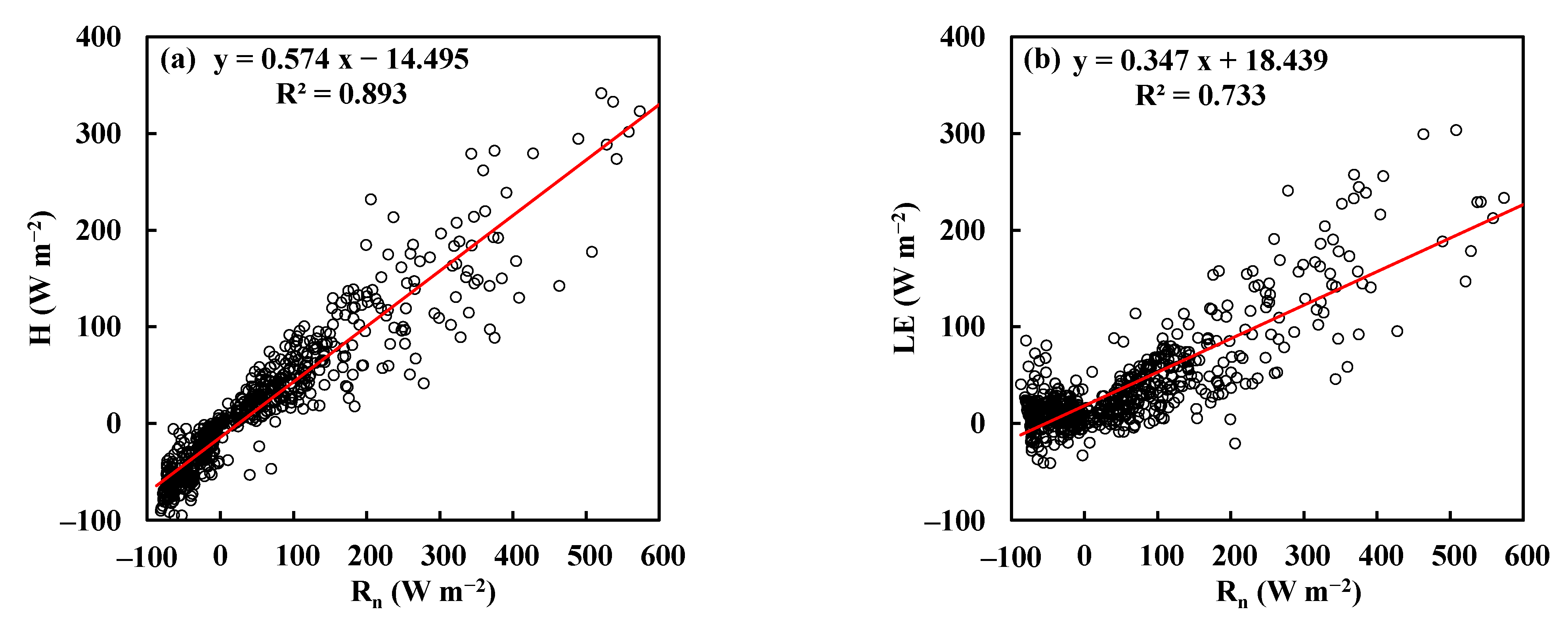
Figure 2 plots the relationship between Rn and H, LE, G, and H+LE+G above this peat bog site. As seen in Figure 2, about 43% of the net radiation was used for warming the air and about 34% of the energy was distributed to evapotranspiration; 21% of the energy was transported to the ground; and the overall energy closure rate was about 98% after data selection using the energy closure condition. Compared with the grassland site, much more energy (21% vs. 8%) was directed into the ground due to a shorter vegetation canopy height. The regression analyses of Figure 2 are also listed in Table 2.
2.3. Forest
This montane forest is part of the National Taiwan University Experimental Forest located in Sitou, Nantou county, central Taiwan. The area of this forest is about 2500 ha and the altitude ranges from 800 to 2000 m. Two meteorological towers (A and B; elevation around 1200 m) were built on the Japanese cedar (Cryptomeria japonica) forest area. The area of this Cryptomeria is 80 ha with an average slope of 13.6°. The average canopy height was about 26 m. The coordinates of tower A (original tower) are 23°39′50.1″ N, 120°47′46.4″ E, and 1252 m above sea level; the location of tower B (new tower) is 64 m away from tower A, and the coordinates are 23°39′51.09″ N, 120°47′44.57″ E, and 1233 m above sea level. The heights of tower A and B were 35 and 40 m, respectively. The climate of this site is warm and humid. The average annual temperature, humidity, and precipitation are 16.6 °C, 89%, and 2635 mm, respectively. In this humid experimental region, fog often occurs in the afternoons in autumn and winter.
For this study, the flux data collected on tower A by the open-path EC system at 28 m above the ground was used. The EC system consisted of a three-dimensional sonic anemometer (CSAT3) and an open-path infrared gas analyzer (Li-7500). The 10 Hz analog signals were simultaneously collected by a data logger (CR3000) and were then averaged every 30 min. In addition, a net radiometer (NR-LITE) and rain gauge (TE525MM) were installed at 27.5 m to measure net radiation and precipitation. A temperature and humidity probe (HMP45C) and a precision infrared temperature sensor (IRTS-P) were installed at 28 m to measure air temperature, relative humidity, and canopy surface temperature. All of the above sensors were connected to a data logger (CR23X). The sampling rate for these sensors was 30 s and the averaging period was 30 min. The data were collected from May 22, 2009 to July 31, 2010. The site and instrumentation features are summarized in Table 3.
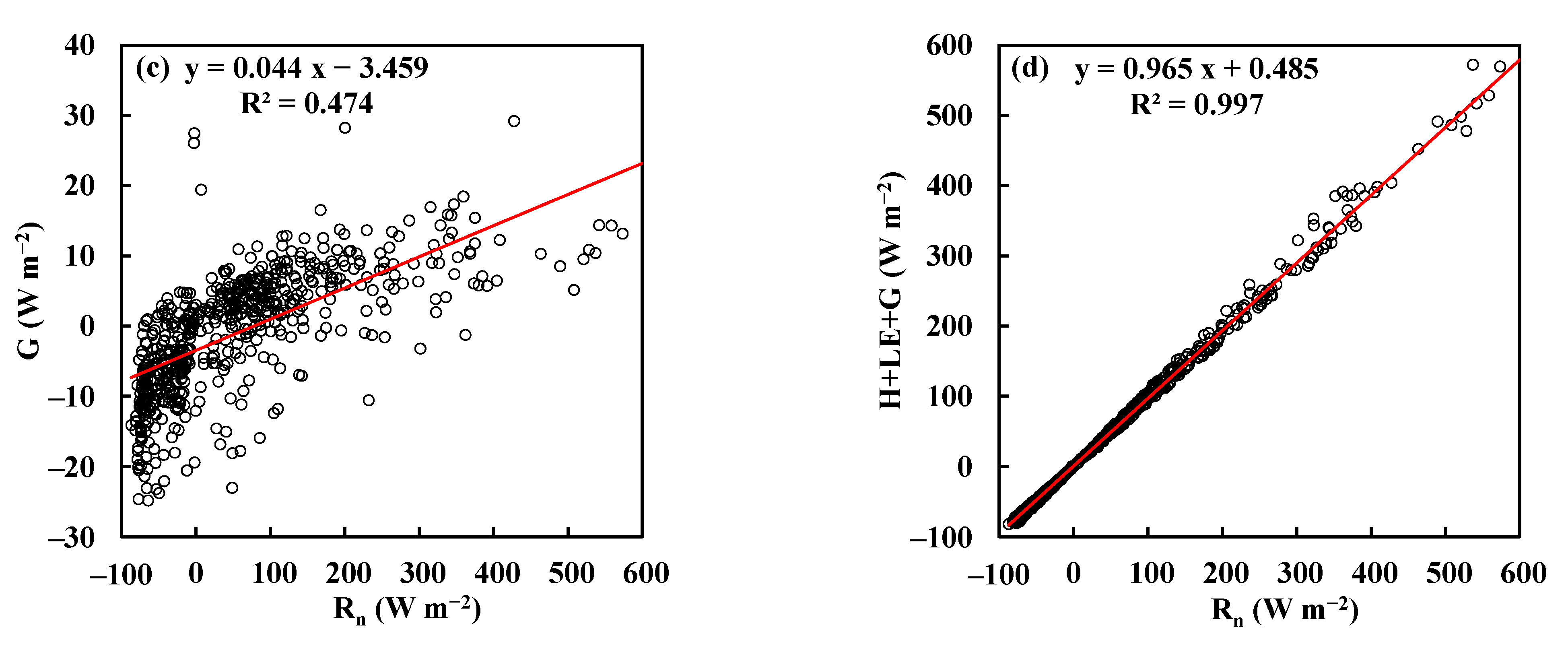
The scatter plots between Rn and H, LE, G, and H+LE+G above the forest site are shown in Figure 3. For this site, the energy partitions for H and LE were about 57% and 35%, respectively; only 4% of the energy was transported into the ground due to the high forest canopy; and the energy closure rate was 97%. These analyses for energy partitions above the forest site are also summarized in Table 2.
3. Methodology
3.1. Penman–Monteith Equation
The P–M equation [3] is a widely used method for calculating water vapor flux and can be expressed as follows:
where γ (= CpP/0.622Lv) is the psychrometric constant (kPa K−1), Cp is the specific heat of air (J kg−1 K−1), P is the atmospheric pressure (kPa), Lv is the latent heat of evaporation (J kg−1), Δ is the slope of the saturated vapor pressure (kPa K−1) calculated at Ta, D is the vapor pressure deficit (kPa), rc is the canopy resistance (s m−1), and rav is the aerodynamic resistance (s m−1).
The aerodynamic resistance can be calculated by:
where k (= 0.4) is the von Karman constant, U is the mean wind speed (m s−1), z is the measurement height, zo is the surface roughness for momentum (≈ 0.1 h, h is canopy height), and zov is the surface roughness for water vapor (≈ 0.01 h,).
Under the framework of the P–M equation, the sensible heat flux is simply calculated by the surface energy balance equation:
In order to apply the P–M equation, the canopy resistance must be determined (or known) a priori. In this study, data from each site were divided into two parts. The first 25% of the data was used for determining rc. Here, the rc value, which could result in a minimum RMSE (root mean square error) between the observed LE and the predicted LE by Equation (1), was the one adopted. The remaining 75% of the data was then used for evaluating the performance of the P–M equation with this rc value. The determined rc values for the grassland, peat bog, and forest sites were 60, 63, and 134 (s m−1), respectively. These rc values for the three sites are also listed in Table 1.
3.2. Priestley–Taylor Equation
Priestley and Taylor [7] suggested that the actual evapotranspiration is proportional to the equilibrium evaporation (LEeq) and can be calculated as
where α is the P–T constant. The P–T equation mainly uses the empirical parameter (α) to compensate for the effects of vapor pressure deficit and canopy resistance considered in the P–M equation [8,9,26]. For wet surfaces, α is generally taken as 1.26 [27]. In the framework of the P–T equation, the sensible heat flux is also calculated by the surface energy balance equation, i.e., Equation (3).
As with the P–M equation, there is one parameter (i.e., α) that needs to be determined before the P–T equation can be applied. Again, the first 25% of the data was used for determining α; the remaining 75% was then used for evaluating the performance of the P–T equation. The P–T constant was determined by performing a linear regression (the intercept was forced to be zero) between the observed LE and the equilibrium evaporation, LEeq. The α values for the grassland, peat bog, and forest sites were found to be 0.962, 0.956, and 0.692, respectively. These values indicate that the evapotranspiration at the grassland and peat bog sites are both close to the equilibrium evaporation, but the forest’s evapotranspiration is only around 70% of LEeq. This value is close to the α values (0.74 and 0.64) of the spruce forest and Scots Pine forest in dry conditions [28]. These α values for the three sites are also summarized in Table 1.
3.3. Non-Parametric Method
The non-parametric method proposed by Liu et al. [1] takes the Hamilton’s principle [11] as the core for the derivation. They assumed that the atmospheric system is a closed system and potential energy is independent of velocity and time. The net radiation is considered as potential energy. On the other hand, H, LE, and G are considered as kinetic energy. Using Lagrange’s principle, the equations for calculating H and LE are:
where σ (= 5.67 × 10⁻⁸) is the Stefan–Boltzmann constant (W m−2 K−4), Ts is the surface temperature (K), Ta is the air temperature (K), and ε is the land surface emissivity. In this study, ε for grassland, peat bog, and forest are 0.95, 0.99, and 0.98, respectively. The parameters required in the non-parametric method are Rn, G, Ts, and Ta, which can be easily measured. No additional empirical or semi-empirical parameter is required.
I II III
On the righthand side of equation (6), the first term (I) is the equilibrium evaporation (LEeq); the second term (II) accounts for the energy adjustment by the long-wave radiation difference between the surface and atmosphere; and the third term (III) represents the flux change caused by the ground heat flux and the temperature difference between the surface and the air. Generally speaking, during the daytime, term I is the major component contributing to LE and term III is minor More details about the derivation and the principle can be found in Liu et al. [1].
4. Results and Discussion
4.1. Performances of P–M, P–T, and N-P Methods
In this section, performances of the three methods for estimating LE and H above the three sites are presented.
4.1.1. Grassland
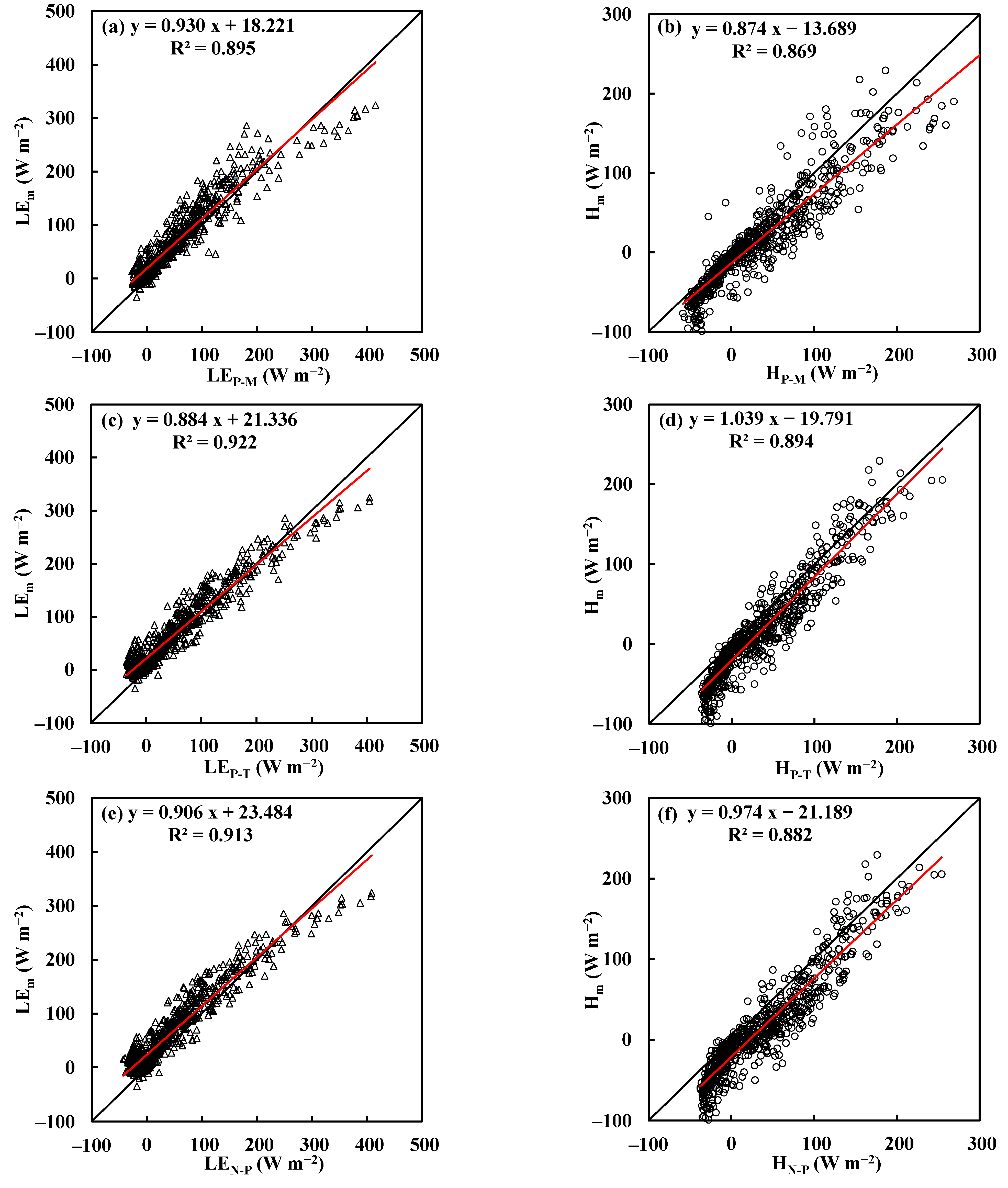
Figure 4 shows the comparisons between the measured and model-predicted LE and H values above the grassland. The regression analyses between measured and model-predicted fluxes are also summarized in Table 3. Figure 4 and Table 3 reveal that all three of the models can predict both LE (R2 between 0.90–0.92; RMSE around 30 W m−2) and H (R2 between 0.87–0.89; RMSE around 30 W m−2) accurately above the grassland site.
To further examine model performance, we plotted the measured and model-predicted LE and H values as a function of available energy (Rn − G) at the grassland, as shown in Figure 5. For the cases of low available energy (Rn − G < 300), all three models resulted in similar and slightly underestimated LE values. This indicated that the actual evapotranspiration rate was slightly higher than the equilibrium evaporation rate when the available energy was small. This extra evapotranspiration was due to the demand of unsaturated atmosphere.
4.1.2. Peat Bog
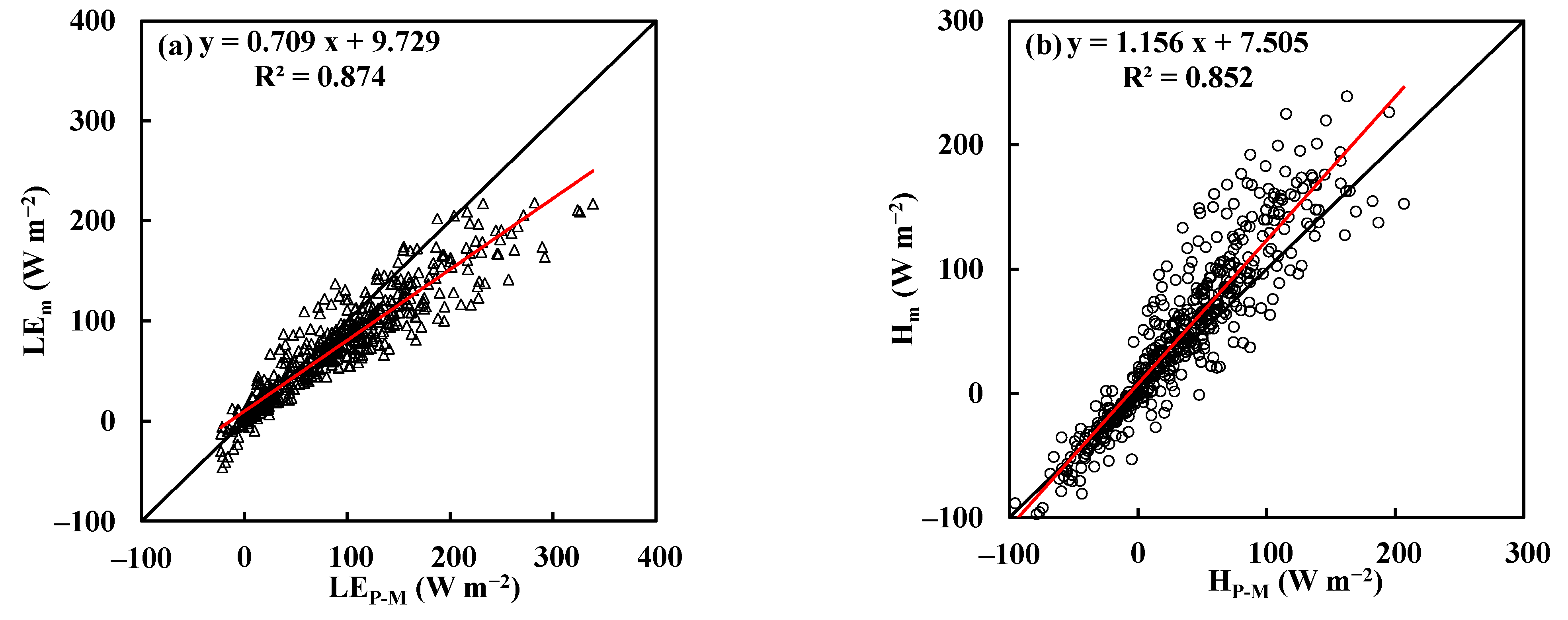
The comparisons between measured and model-predicted LE and H above the peat bog are shown in Figure 6. The regression analyses between measured and model-predicted fluxes are also listed in Table 3. From Figure 6 and Table 3, it is clear that all of the LE predictions from the three models are in agreement with the measurements (R2 between 0.82–0.89); similar results are also found for H (R2 between 0.79–0.90). The RMSEs for LE (between 29–33 W m−2) and H (between 27–31 W m−2) for each of the models are approximately the same as those at the grassland site. Overall, these three models performed well above the peat bog site.
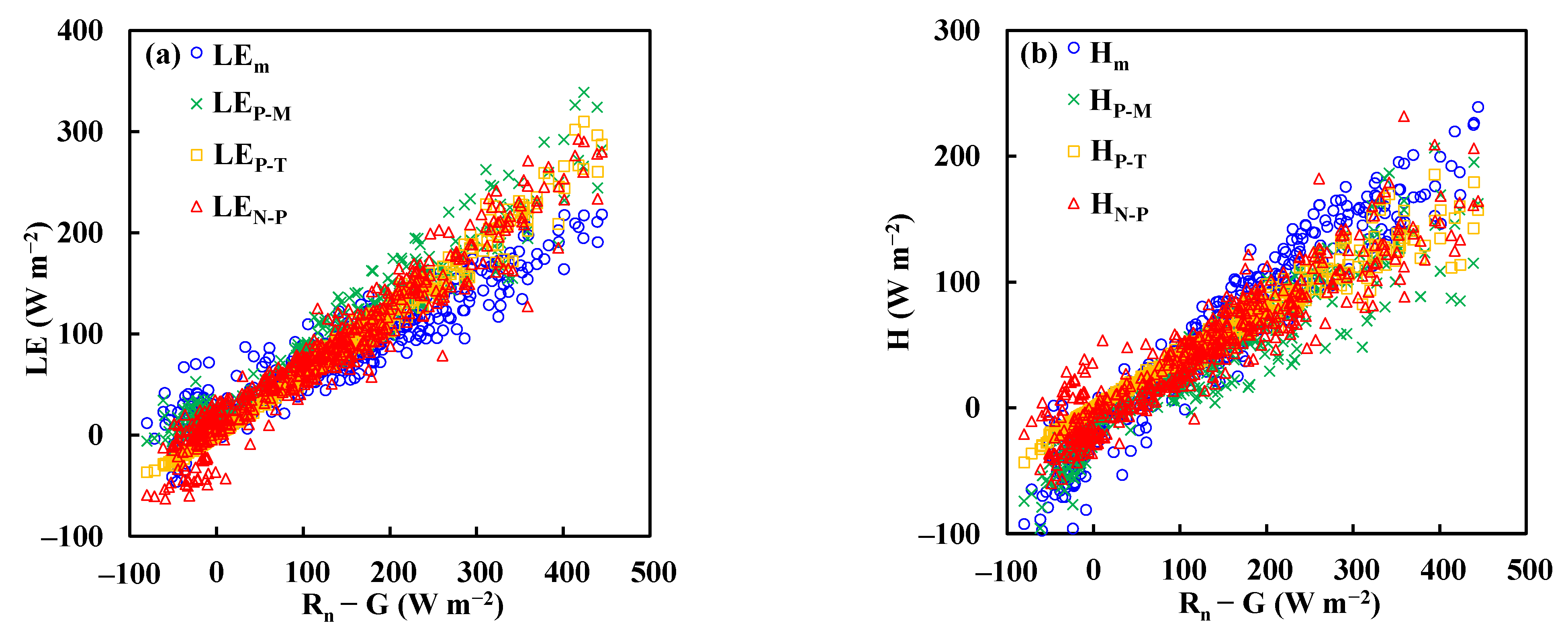
Further model performance evaluation was done by plotting the measured and model-predicted LE and H values as a function of available energy (Rn − G) at the peat bog (Figure 7). From Figure 7 it appears for the cases of high available energy (Rn − G > 300), all three of the models slightly overpredicted LE. This shows that the actual evapotranspiration rate was slightly lower than the equilibrium evaporation rate when the available energy was large. This reduction of evapotranspiration might have been caused by resistance from the vegetation in order to reduce water loss during higher air temperature and radiation.
4.1.3. Forest
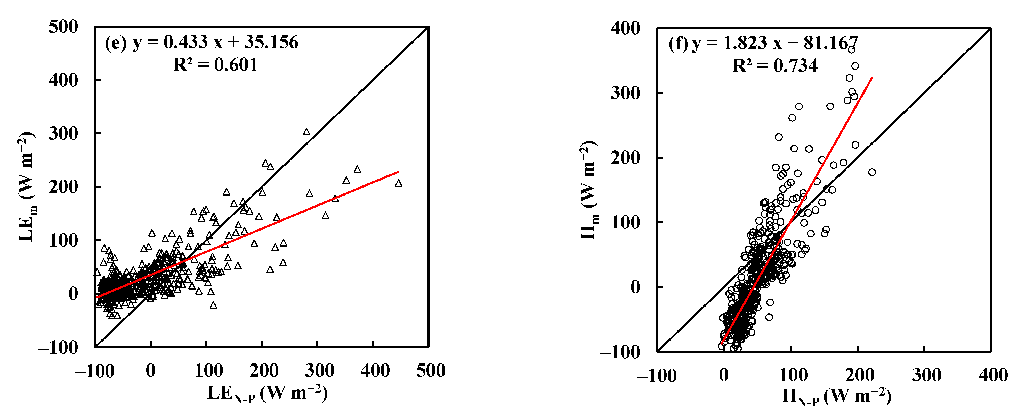
The scatter plots of measured and model-predicted LE and H above the forest are shown in Figure 8. The regression analyses between measured and model predicted fluxes are also listed in Table 3. From Figure 8 and Table 3, both the P–M and P–T equations appear to have reproduced LE and H accurately (RMSEs around 30 W m−2) above the forest site. However, the LE and H predicted by the N-P method were not in agreement with the measurements (both RMSEs were around 65 W m−2).
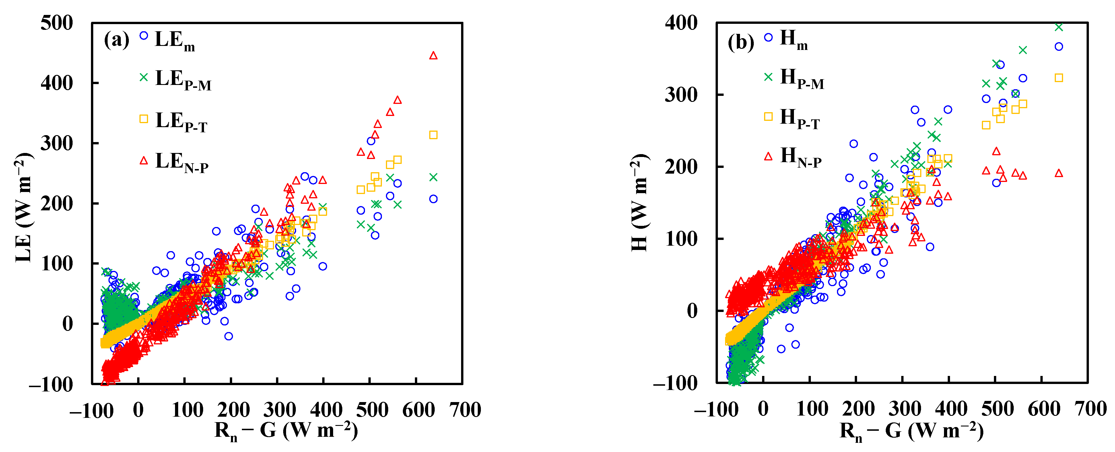
Figure 9 shows the measured and model-predicted LE and H values as a function of available energy (Rn-G) at the forest site. In Figure 9, it appears that in the cases of high available energy (Rn − G > 400), the N-P method overpredicted LE and underestimated H. This reveals that the actual evapotranspiration rate was much lower than the equilibrium evaporation rate when the available energy was large. Similar to the peat bog site (although the magnitude was larger), this reduction of evapotranspiration might have been be caused by resistance from the vegetation in order to avoid a large amount of water loss (physiological control) during high air temperature and radiation.
4.2. Limitation of the Non-Parametric Method
To further investigate the limitation and accuracy of the non-parametric method, in this section we analyze the contribution of each term in the N-P method.
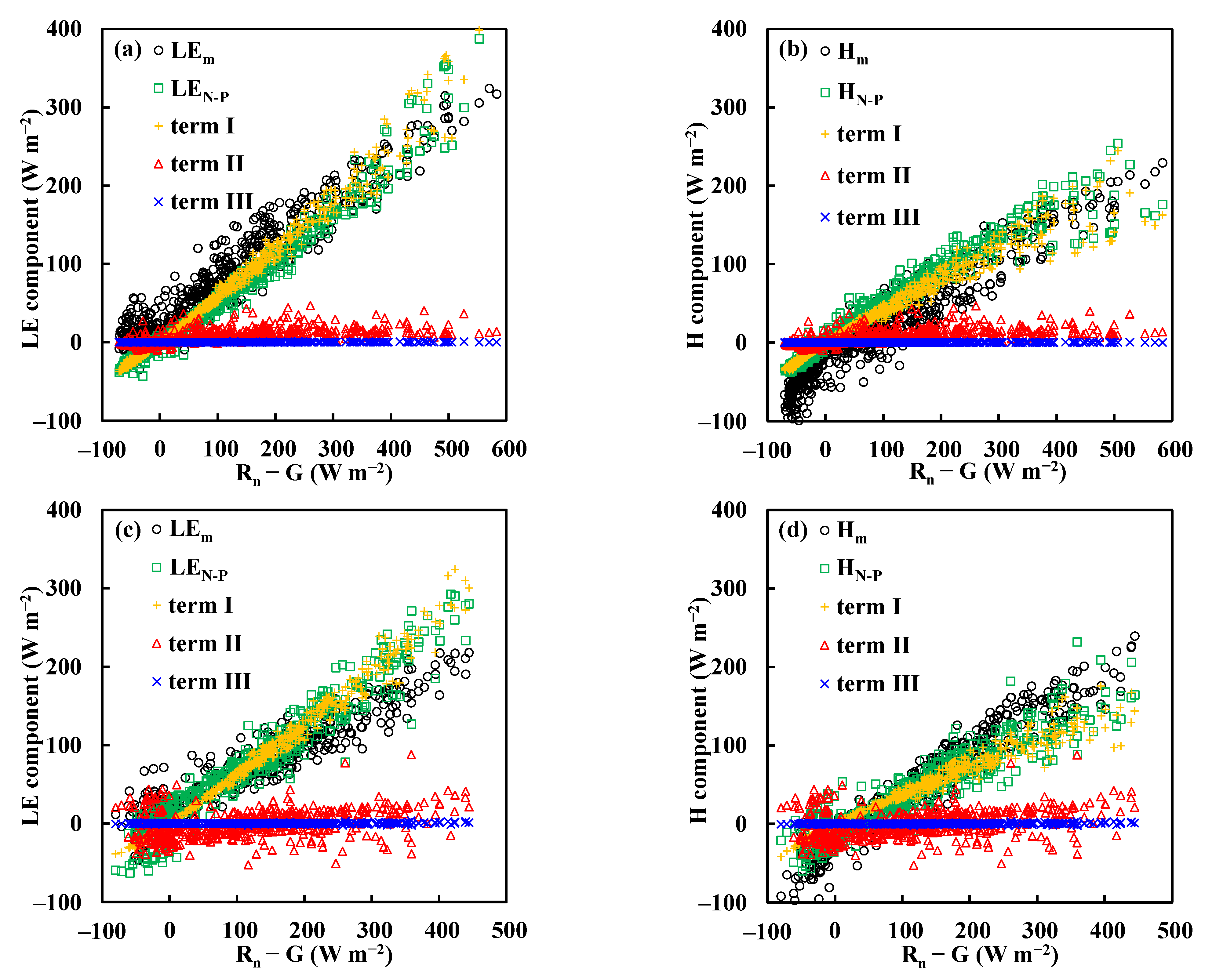
Figure 10 plots the three terms in the non-parametric method as a function of Rn-G for latent heat and sensible heat fluxes above the grassland, peat bog, and forest. For all three sites, term III is very small and close to zero. Hence, term III can be neglected.
Using the P–T equation and replacing LE with αLEeq in Equation (6), and neglecting term III, we have
Now by replacing LEeq with LE/α in Equation (6), we get
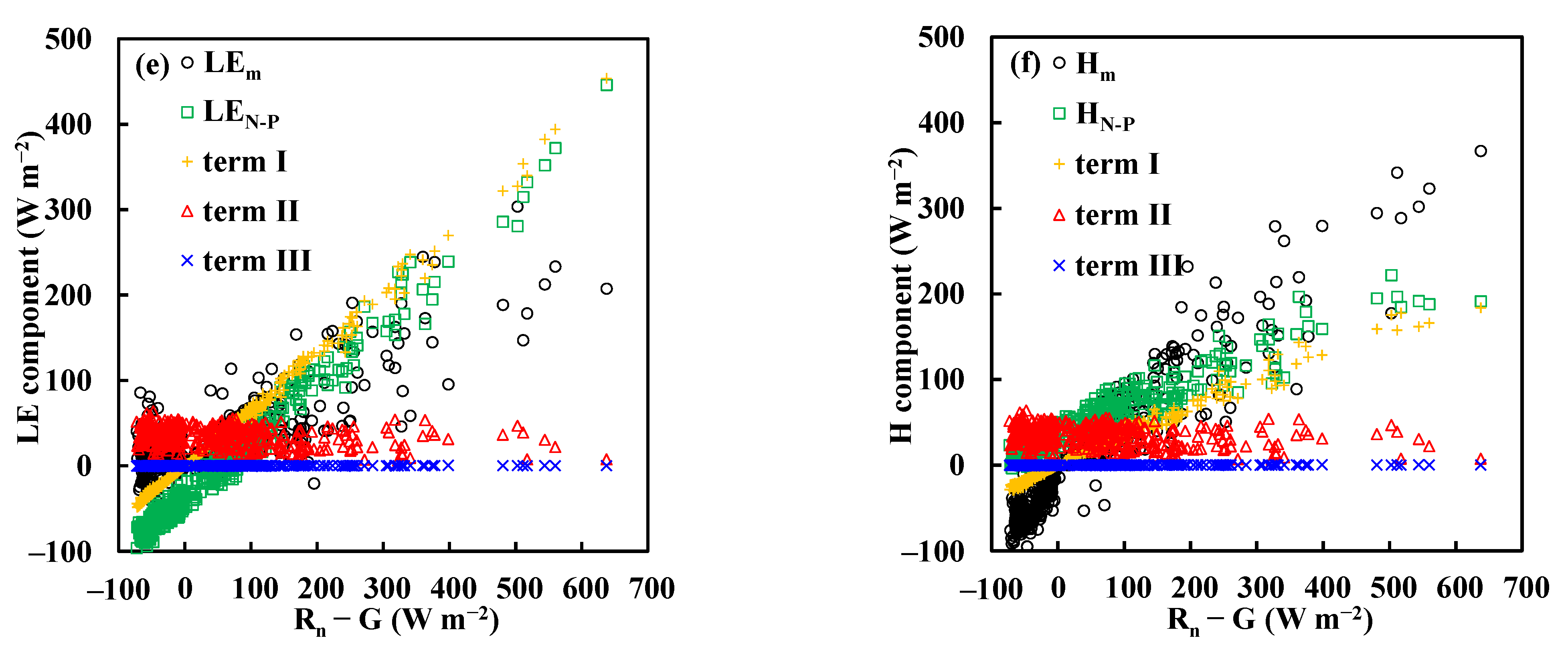
Equations (7) or (8) represent the condition that should be satisfied if the N-P method is applied for estimating LE. Figure 11 shows the relationship between term II and LEeq along with the measured LE for the three sites. In Figure 11, the slopes for the grassland and peat bog sites are positive, but those for the forest site are negative. This is because when Rn for the forest site is large, most of the energy (57%, see Table 2) is distributed to H for warming up the air; hence, the difference between Ts and Ta is reduced which results in a smaller term II. Figure 11 also reveals that term II is about ±10% (from −0.051 to 0.083) of the equilibrium evapotranspiration (Figure 11a,c,e).
From the linear regression analyses shown in Figure 11 and Equations (7) and (8), we found that the α values for the three sites ranged from 0.89–1.05 (see Table 4). This means that when applying the N-P method to estimate LE, the actual evapotranspiration should be around 0.89–1.05 times the equilibrium evapotranspiration. Both the grassland and peat bog sites met this condition (both α = 0.96). However, the P–T constant at the forest is only 0.69; hence, Equations (7) and (8) are not satisfied. This explains why the N-P method performed well for the grassland and peat bog, but not so well for the forest.
The N-P method assumes that “the system of liquid water in leaf tissues and the water vapor in the atmosphere tends to evolve towards a potential equilibrium as quickly as possible by maximization of the transpiration rate” [29]; however, a system like the forest, which tends to reduce the transpiration rate during high air temperature and radiation in order to avoid a large amount of water loss, would violate this assumption and the N-P method is not suitable for this kind of ecosystem. As previously mentioned, the α values of the spruce forest and Scots Pine forest in dry conditions are 0.74 and 0.64, respectively [28]. This implies that the N-P method is not suitable for these forests either.
4.3. Sensitivity of the N-P Method on Surface Temperature
The advantage of the N-P method is that experimental parameters (such as rc and α) are not needed. However, compared with the P–M and P–T equations, this method requires one additional input, Ts. Hence, it is worth noting the sensitivity of the N-P method to the change of Ts.
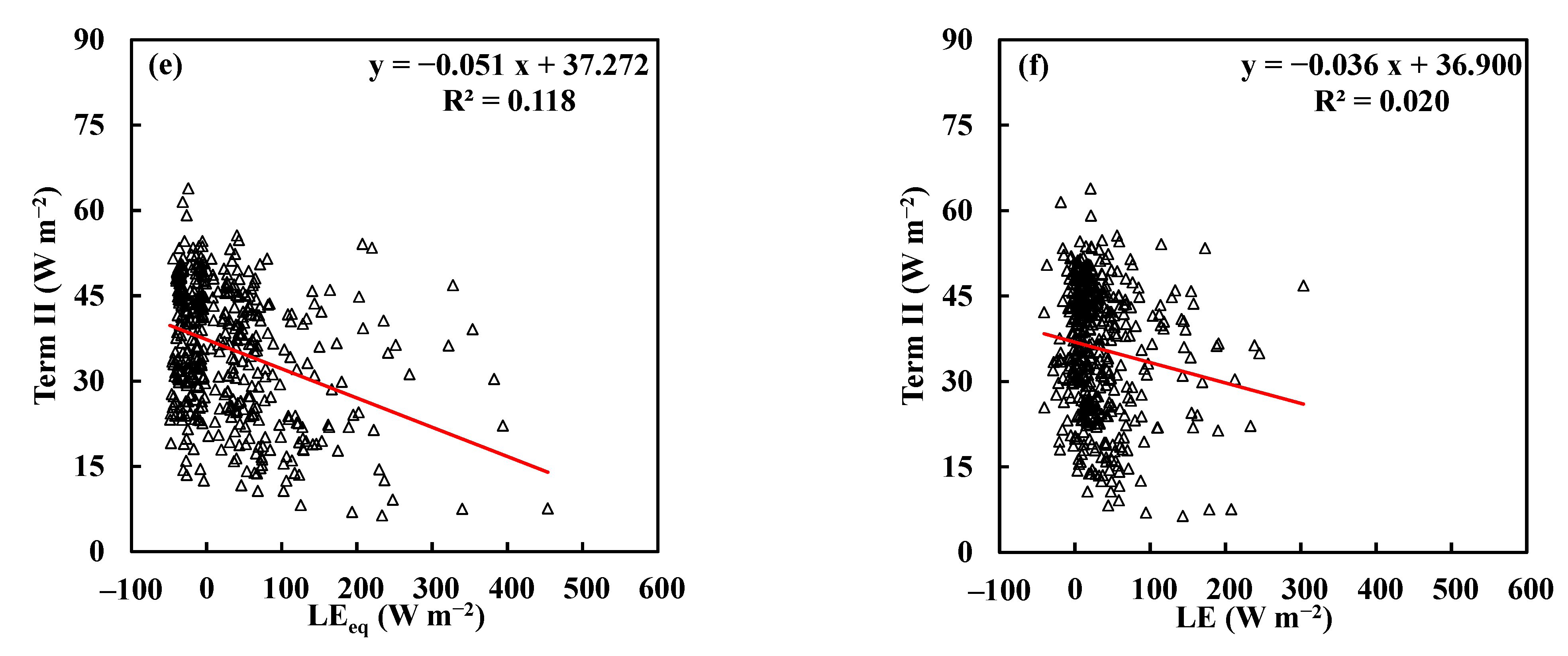
Taking the derivatives of H (Equation (5)) and LE (Equation (6)) with respect to Ts, we have
Equations (9) and (10) describe how predicted H and LE are changed with a unit change of Ts. From Equation (10), it is clear that ∂LE/∂Ts is a function of Ts and G. From field measurements of the three sites, Ts is in the range of −5 to 30 °C, and G is between −20 and 100 (W m−2). From these conditions, with ε = 0.95, Figure 12 plots ∂LE/∂Ts and ∂H/∂Ts as a function of Ts under different G values. Figure 12 reveals that with a one-degree change in Ts, the predicted LE and H are only changed by 4 to 6 (W m−2). In other words, the LE predicted by the N-P method is not sensitive to the uncertainty of Ts measurements.
5. Conclusions
Field measurements above grassland, peat bog, and forest were used to investigate the accuracy and limitations of the non-parametric method in predicting evapotranspiration. The model’s performance was also compared with those of the Penman–Monteith and Priestley–Taylor equations. Our results demonstrate the following:
- (1)
- The evapotranspiration rates above the grassland and peat bog were close to the equilibrium evaporation (P–T constant ≈ 0.96). The forest’s evapotranspiration rate was 69% of the equilibrium evaporation, and about 60% of the net radiation energy was distributed to sensible heat flux.
- (2)
- Both the P–M and P–T equations performed well at estimating water vapor and sensible heat fluxes for all of the three sites. However, the canopy resistance in the P–M equation and the Priestley–Taylor constant in the P–T equation must be known a priori.
- (3)
- The water vapor flux predictions by the N-P method were in agreement with the measurements above the grassland and peat bog. However, this was not the case for the forest site.
- (4)
- Our analysis shows that with one degree of change in Ts, the predicted LE is only changed by 4 to 6 (W m−2). Hence, the LE predictions by the N-P method are not sensitive to the uncertainty of Ts measurements.
- (5)
- Field measurements from the three sites reveal that the second term of the N-P method is about ±10% (from −0.05 to 0.08) of the equilibrium evapotranspiration. For applying the N-P method to estimate LE, the actual evapotranspiration of the site should be around 0.89–1.05 times the equilibrium evapotranspiration.
In theory, the non-parametric method assumes that at the local thermal equilibrium environment (i.e., Ta = Ts), the actual evaporation rate is the equilibrium evaporation, and that when the surface temperature is increased (i.e., Ts > Ta), the actual evaporation rate will be dropped since some energy is used for sensible heat flux. Our field measurements show that this energy adjustment is small (around 10% of LEeq). Hence, the N-P method is only suitable for a system where the actual evaporation rate is close to the equilibrium evaporation (difference within ±10%). For a system (such as the forest) where the actual LE is much less than LEeq, this method will not work.
Author Contributions
C.-I.H. conceived the research idea; C.-I.H., C.-J.C., and I.-H.H. performed the model simulations; G.K. performed the grassland and peat bog experiments; C.-I.H. performed the forest experiment; all authors took part in the discussion, data analysis, and interpretation of the data and model predictions; C.-I.H., C.-J.C., and I.-H.H. wrote the manuscript. All authors reviewed the manuscript. All authors have read and agreed to the published version of the manuscript.
Funding
This work was supported, in part, by the Ministry of Science and Technology, Taiwan [grant number: MOST 110-2111-M-002-011] and the Core Research Project, National Taiwan University [project number: NTU-CC-110L890903; NTU-CC-111L890903].
Data Availability Statement
The data used to support the findings of this study are available from the corresponding author upon request.
Acknowledgments
The authors are grateful to Shih-Min Cheng for her great help with the forest experiment.
Conflicts of Interest
The authors declare no conflict of interest.
Abbreviations
| Symbol | Description |
| Cp | specific heat of air (J kg−1 K−1) |
| D | vapor pressure deficit (kPa) |
| G | ground heat flux (W m−2) |
| H | sensible heat flux (W m−2) |
| k | von Karman constant (= 0.4) |
| LE | latent heat flux (W m−2) |
| Lv | latent heat of evaporation (J kg−1) |
| P | atmospheric pressure (kPa) |
| Rn | net radiation (W m−2) |
| rc | canopy resistance (s m−1) |
| rav | aerodynamic resistance (s m−1) |
| Ta | air temperature (°C) |
| Ts | surface temperature (°C) |
| U | wind speed (m s−1) |
| z | measurement height (m) |
| zo | surface roughness for momentum (m) |
| zov | surface roughness for water vapor (m) |
| α | Priestly–Taylor constant |
| γ | psychrometric constant (kPa K−1) |
| Δ | slope of the saturated vapor pressure (kPa K−1) |
| ε | land surface emissivity |
| σ | Stefan–Boltzmann constant (= 5.67 × 10⁻⁸) (W m−2 K−4) |
References
- Liu, Y.; Hiyama, T.; Yasunari, T.; Tanaka, H. A nonparametric approach to estimating terrestrial evaporation: Validation in eddy covariance sites. Agric. For. Meteorol. 2012, 157, 49–59. [Google Scholar] [CrossRef]
- Shuttleworth, W.J. Putting the “vap” into evaporation. Hydrol. Earth Syst. Sci. 2007, 11, 210–244. [Google Scholar] [CrossRef] [Green Version]
- Monteith, J.L. Evaporation and surface temperature. Q. J. R. Meteor. Soc. 1981, 107, 1–27. [Google Scholar] [CrossRef]
- Raupach, M.R. Influences of local feedbacks on land–air exchanges of energy and carbon. Glob. Change Biol. 1998, 4, 477–494. [Google Scholar] [CrossRef]
- Irmak, S.; Mutiibwa, D. On the dynamics of canopy resistance: Generalized linear estimation and relationships with primary micrometeorological variables. Water Resour. Res. 2010, 46, 8. [Google Scholar] [CrossRef] [Green Version]
- Lin, B.S.; Lei, H.; Hu, M.C.; Visessri, S.; Hsieh, C.I. Canopy resistance and estimation of evapotranspiration above a humid cypress forest. Adv. Meteorol. 2020, 2020, 4232138. [Google Scholar] [CrossRef] [Green Version]
- Priestley, C.H.B.; Taylor, R.J. On the assessment of surface heat flux and evaporation using large-scale parameters. Mon. Weather Rev. 1972, 100, 81–92. [Google Scholar] [CrossRef]
- Pereira, A.R. The Priestley–Taylor parameter and the decoupling factor for estimating reference evapotranspiration. Agric. For. Meteorol. 2004, 125, 305–313. [Google Scholar] [CrossRef]
- Bottazzi, M.; Bancheri, M.; Mobilia, M.; Bertoldi, G.; Longobardi, A.; Rigon, R. Comparing evapotranspiration estimates from the geoframe-prospero model with Penman–Monteith and Priestley-Taylor approaches under different climate conditions. Water 2021, 13, 1221. [Google Scholar] [CrossRef]
- Qiu, R.J.; Liu, C.W.; Cui, N.B.; Wu, Y.J.; Wang, Z.C.; Li, G. Evapotranspiration estimation using a modified Priestley-Taylor model in a rice-wheat rotation system. Agric. Water Manag. 2019, 224, 105755. [Google Scholar] [CrossRef]
- Magyari, E.; Keller, B. Hamiltonian description of the heat conduction. Heat Mass Transf. 1999, 34, 453–459. [Google Scholar] [CrossRef]
- Pan, X.; Liu, Y.; Fan, X. Satellite retrieval of surface evapotranspiration with nonparametric approach: Accuracy assessment over a semiarid region. Adv. Meteorol. 2016, 2016, 1584316. [Google Scholar] [CrossRef] [Green Version]
- Pan, X.; Liu, Y.; Gan, G.; Fan, X.; Yang, Y. Estimation of evapotranspiration using a nonparametric approach under all sky: Accuracy evaluation and error analysis. IEEE J. Sel. Top. Appl. Earth Obs. Remote Sens. 2017, 10, 2528–2539. [Google Scholar] [CrossRef]
- Pan, X.; You, C.; Liu, Y.; Shi, C.; Han, S.; Yang, Y.; Hu, J. Evaluation of satellite-retrieved evapotranspiration based on a nonparametric approach over an arid region. Int. J. Remote Sens. 2020, 41, 7605–7623. [Google Scholar] [CrossRef]
- Wu, B.; Zhu, W.; Yan, N.; Xing, Q.; Xu, J.; Ma, Z.; Wang, L. Regional actual evapotranspiration estimation with land and meteorological variables derived from multi-source satellite data. Remote Sens. 2020, 12, 332. [Google Scholar] [CrossRef] [Green Version]
- Yang, Y.; Su, H.; Qi, J. A critical evaluation of the nonparametric approach to estimate terrestrial evaporation. Adv. Meteorol. 2016, 2016, 5343718. [Google Scholar] [CrossRef] [Green Version]
- Jaksic, V.; Kiely, G.; Albertson, J.; Oren, R.; Katul, G.; Leahy, P.; Byrne, K.A. Net ecosystem exchange of grassland in contrasting wet and dry years. Agric. Forest. Meteorol. 2006, 139, 323–334. [Google Scholar] [CrossRef]
- Lawton, D.; Leahy, P.; Kiely, G.; Byrne, K.A.; Calanca, P. Modeling of net ecosystem exchange and its components for a humid grassland ecosystem. J. Geophys. Res. Biogeosciences 2006, 111, G04013. [Google Scholar] [CrossRef] [Green Version]
- Byrne, K.A.; Kiely, G.; Leahy, P. CO2 fluxes in adjacent new and permanent temperate grasslands. Agric. For. Meteorol. 2005, 135, 82–92. [Google Scholar] [CrossRef]
- Peichl, M.; Leahy, P.; Kiely, G. Six-year stable annual uptake of carbon dioxide in intensively managed humid temperate grassland. Ecosystems 2011, 14, 112–126. [Google Scholar] [CrossRef]
- Lewis, C.; Albertson, J.; Xu, X.; Kiely, G. Spatial variability of hydraulic conductivity and bulk density along a blanket peatland hillslope. Hydrol. Process. 2012, 26, 1527–1537. [Google Scholar] [CrossRef]
- Laine, A.; Sottocornola, M.; Kiely, G.; Byrne, K.A.; Wilson, D.; Tuittila, E.S. Estimating net ecosystem exchange in a patterned ecosystem: Example from blanket bog. Agric. For. Meteorol. 2006, 138, 231–243. [Google Scholar] [CrossRef]
- Sottocornola, M.; Laine, A.; Kiely, G.; Byrne, K.A.; Tuittila, E.S. Vegetation and environmental variation in an Atlantic blanket bog in South-western Ireland. Plant Ecol. 2009, 203, 69–81. [Google Scholar] [CrossRef]
- Sottocornola, M.; Kiely, G. Hydro-meteorological controls on the CO2 exchange variation in an Irish blanket bog. Agric. For. Meteorol. 2010, 150, 287–297. [Google Scholar] [CrossRef]
- McVeigh, P.; Sottocornola, M.; Foley, N.; Leahy, P.; Kiely, G. Meteorological and functional response partitioning to explain interannual variability of CO2 exchange at an Irish Atlantic blanket bog. Agric. For. Meteorol. 2014, 194, 8–19. [Google Scholar] [CrossRef]
- Gong, X.; Qiu, R.; Ge, J.; Bo, G.; Ping, Y.; Xin, Q.; Wang, S. Evapotranspiration partitioning of greenhouse grown tomato using a modified Priestley–Taylor model. Agric. Water Manag. 2021, 247, 106709. [Google Scholar] [CrossRef]
- Eichinger, W.E.; Parlange, M.B.; Stricker, H. On the concept of equilibrium evaporation and the value of the Priestley-Taylor coefficient. Water Resour. Res. 1996, 32, 161–164. [Google Scholar] [CrossRef] [Green Version]
- Shuttleworth, W.J.; Calder, I.R. Has the Priestley-Taylor Equation Any Relevance to Forest Evaporation? J. Appl. Meteorol. 1979, 18, 639–646. [Google Scholar] [CrossRef]
- Wang, J.; Bras, R.L.; Lerdau, M.; Salvucci, G.D. A maximum hypothesis of transpiration. J. Geophys. Res. Biogeosciences 2007, 112, W03010. [Google Scholar] [CrossRef]
Figure 1.
Scatter plots between Rn and H (a), LE (b), G (c), and H+LE+G (d) above the grassland.

Figure 2.
Scatter plots between Rn and H (a), LE (b), G (c), and H+LE+G (d) above the peat bog.

Figure 3.
Scatter plots between Rn and H (a), LE (b), G (c), and H+LE+G (d) above the forest.


Figure 4.
Comparisons of measured and predicted LE and H by the P–M equation (a,b), P–T equation (c,d), and N-P method (e,f) above the grassland. The 1:1 line is also shown.
Figure 4.
Comparisons of measured and predicted LE and H by the P–M equation (a,b), P–T equation (c,d), and N-P method (e,f) above the grassland. The 1:1 line is also shown.

Figure 5.
Scatter plots of measured and model-predicted LE (a) and H (b) as a function of available energy (Rn − G) above the grassland.
Figure 5.
Scatter plots of measured and model-predicted LE (a) and H (b) as a function of available energy (Rn − G) above the grassland.

Figure 6.
Comparisons of measured and predicted LE and H by the P–M equation (a,b), P–T equation (c,d), and non-parametric method (e,f) above the peat bog. The 1:1 line is also shown.
Figure 6.
Comparisons of measured and predicted LE and H by the P–M equation (a,b), P–T equation (c,d), and non-parametric method (e,f) above the peat bog. The 1:1 line is also shown.


Figure 7.
Scatter plots of measured and model-predicted LE (a) and H (b) as a function of available energy (Rn − G) above the peat bog.
Figure 7.
Scatter plots of measured and model-predicted LE (a) and H (b) as a function of available energy (Rn − G) above the peat bog.

Figure 8.
Comparisons of measured and predicted LE and H by the P–M equation (a,b), P–T equation (c,d), and non-parametric method (e,f) above the forest. The 1:1 line is also shown.
Figure 8.
Comparisons of measured and predicted LE and H by the P–M equation (a,b), P–T equation (c,d), and non-parametric method (e,f) above the forest. The 1:1 line is also shown.


Figure 9.
Scatter plots of measured and model-predicted LE (a) and H (b) as a function of available energy (Rn − G) above the forest.
Figure 9.
Scatter plots of measured and model-predicted LE (a) and H (b) as a function of available energy (Rn − G) above the forest.

Figure 10.
Scatter plots of the three terms in the non-parametric method as a function of Rn − G for LE and H above the grassland (a,b), peat bog (c,d), and forest (e,f).
Figure 10.
Scatter plots of the three terms in the non-parametric method as a function of Rn − G for LE and H above the grassland (a,b), peat bog (c,d), and forest (e,f).


Figure 11.
Scatter plots of term II as a function of LEeq and measured LE above the grassland (a,b), peat bog (c,d), and forest (e,f).
Figure 11.
Scatter plots of term II as a function of LEeq and measured LE above the grassland (a,b), peat bog (c,d), and forest (e,f).


Figure 12.
(a) ∂LE/∂Ts, (b) ∂H/∂Ts as a function of Ts under different ground heat flux.


Table 1.
Summary of site features and instrumental heights at the grassland, peat bog, and forest.
| Site | Grassland | Peat Bog | Forest |
|---|---|---|---|
| Data period | 1 January 2013–31 December 2013 | 1 January 2013–31 December 2013 | 22 May 2009–31 July 2010 |
| Altitude (m) | 195 | 150 | 1252 |
| Location | 59°59′ N, 8°45′ W | 51°55′ N, 9°55′ W | 23°39′51.09″ N, 120°47′44.57″ E |
| Climate type | Temperate | Temperate | Sub-tropical |
| Annual rainfall (mm) | 1161 | 1834 | 2635 |
| Mean temperature (°C) | 9 | 10.1 | 16.6 |
| Mean humidity (%) | 92 | 82 | 89 |
| Canopy height (m) | 0.3 | 0.1 | 26 |
| Surface emissivity | 0.95 | 0.99 | 0.98 |
| Canopy resistance (s m−1) | 60 | 63 | 134 |
| Priestley–Taylor constant | 0.962 | 0.956 | 0.692 |
| Measurement height (m) | |||
| Eddy covariance system | 5 | 3 | 28 |
| Air temperature & humidity sensor | 5 | 3 | 28 |
| Net radiometer | 4 | 2 | 27.5 |
| Soil heat flux plate | −0.1 | −0.1 | −0.05 |
| Soil thermometer | −0.015, −0.025, −0.075 | −0.1 | −0.05, −0.1 |
| Soil moisture meter | −0.05 | −0.1 | −0.05, −0.1 |
Table 2.
Summary of linear regression between Rn and H, LE, G, and H+LE+G for the grassland, peat bog, and forest sites. Y = aX + b; X is Rn; Y is H, LE, and so on.
Table 2.
Summary of linear regression between Rn and H, LE, G, and H+LE+G for the grassland, peat bog, and forest sites. Y = aX + b; X is Rn; Y is H, LE, and so on.
| Grassland | Peat Bog | Forest | |||||||
|---|---|---|---|---|---|---|---|---|---|
| Flux | a | b | R2 | a | b | R2 | a | b | R2 |
| H | 0.404 | −17.439 | 0.897 | 0.426 | −14.819 | 0.913 | 0.574 | −14.495 | 0.893 |
| LE | 0.481 | 23.329 | 0.907 | 0.342 | 22.239 | 0.876 | 0.347 | 18.439 | 0.733 |
| G | 0.081 | −5.916 | 0.590 | 0.210 | −6.948 | 0.808 | 0.044 | −3.459 | 0.474 |
| H+LE+G | 0.966 | −0.026 | 0.997 | 0.977 | 0.472 | 0.997 | 0.965 | 0.485 | 0.997 |
Table 3.
Summary of regression analysis between measured and model-predicted fluxes at the three sites. Y = aX + b; Y is measured flux; X is predicted flux.
Table 3.
Summary of regression analysis between measured and model-predicted fluxes at the three sites. Y = aX + b; Y is measured flux; X is predicted flux.
| Latent Heat Flux | Sensible Heat Flux | ||||||||
|---|---|---|---|---|---|---|---|---|---|
| Site | Model | a | b | R2 | RMSE | a | b | R2 | RMSE |
| Grassland | P–M | 0.930 | 18.221 | 0.895 | 28.338 | 0.874 | −13.689 | 0.869 | 29.310 |
| P–T | 0.884 | 21.336 | 0.922 | 27.362 | 1.039 | −19.791 | 0.894 | 27.251 | |
| N-P | 0.906 | 23.484 | 0.913 | 29.866 | 0.974 | −21.189 | 0.882 | 30.447 | |
| Peat Bog | P–M | 0.709 | 9.729 | 0.874 | 32.507 | 1.156 | 7.505 | 0.852 | 29.781 |
| P–T | 0.691 | 20.482 | 0.888 | 29.047 | 1.347 | −16.744 | 0.896 | 26.967 | |
| N-P | 0.675 | 18.608 | 0.826 | 33.161 | 1.133 | −1.661 | 0.797 | 31.063 | |
| Forest | P–M | 0.950 | −1.269 | 0.603 | 28.799 | 0.864 | 3.026 | 0.883 | 29.575 |
| P–T | 0.687 | 18.383 | 0.643 | 33.945 | 1.185 | −17.503 | 0.875 | 33.004 | |
| N-P | 0.433 | 35.156 | 0.601 | 66.553 | 1.823 | −81.167 | 0.734 | 64.657 | |
Table 4.
α derived from Equations (7) and (8).
| Site | Grassland | Peat Bog | Forest |
|---|---|---|---|
| α from Equation (7) | 0.929 | 0.917 | 1.051 |
| α from Equation (8) | 0.928 | 0.890 | 1.037 |
Publisher’s Note: MDPI stays neutral with regard to jurisdictional claims in published maps and institutional affiliations. |
© 2022 by the authors. Licensee MDPI, Basel, Switzerland. This article is an open access article distributed under the terms and conditions of the Creative Commons Attribution (CC BY) license (https://creativecommons.org/licenses/by/4.0/).
Share and Cite
MDPI and ACS Style
Hsieh, C.-I.; Chiu, C.-J.; Huang, I.-H.; Kiely, G. Estimation of Latent Heat Flux Using a Non-Parametric Method. Water 2022, 14, 3474. https://doi.org/10.3390/w14213474
AMA Style
Hsieh C-I, Chiu C-J, Huang I-H, Kiely G. Estimation of Latent Heat Flux Using a Non-Parametric Method. Water. 2022; 14(21):3474. https://doi.org/10.3390/w14213474
Chicago/Turabian StyleHsieh, Cheng-I, Cheng-Jiun Chiu, I-Hang Huang, and Gerard Kiely. 2022. "Estimation of Latent Heat Flux Using a Non-Parametric Method" Water 14, no. 21: 3474. https://doi.org/10.3390/w14213474
Note that from the first issue of 2016, this journal uses article numbers instead of page numbers. See further details here.