
Spatial Distribution and Hydrogeochemical Factors Influencing the Occurrence of Total Coliform and E. coli Bacteria in Groundwater in a Hyperarid Area, Ad-Dawadmi, Saudi Arabia

 , , ,
, , ,
Abstract
:1. Introduction
2. Materials and Methods
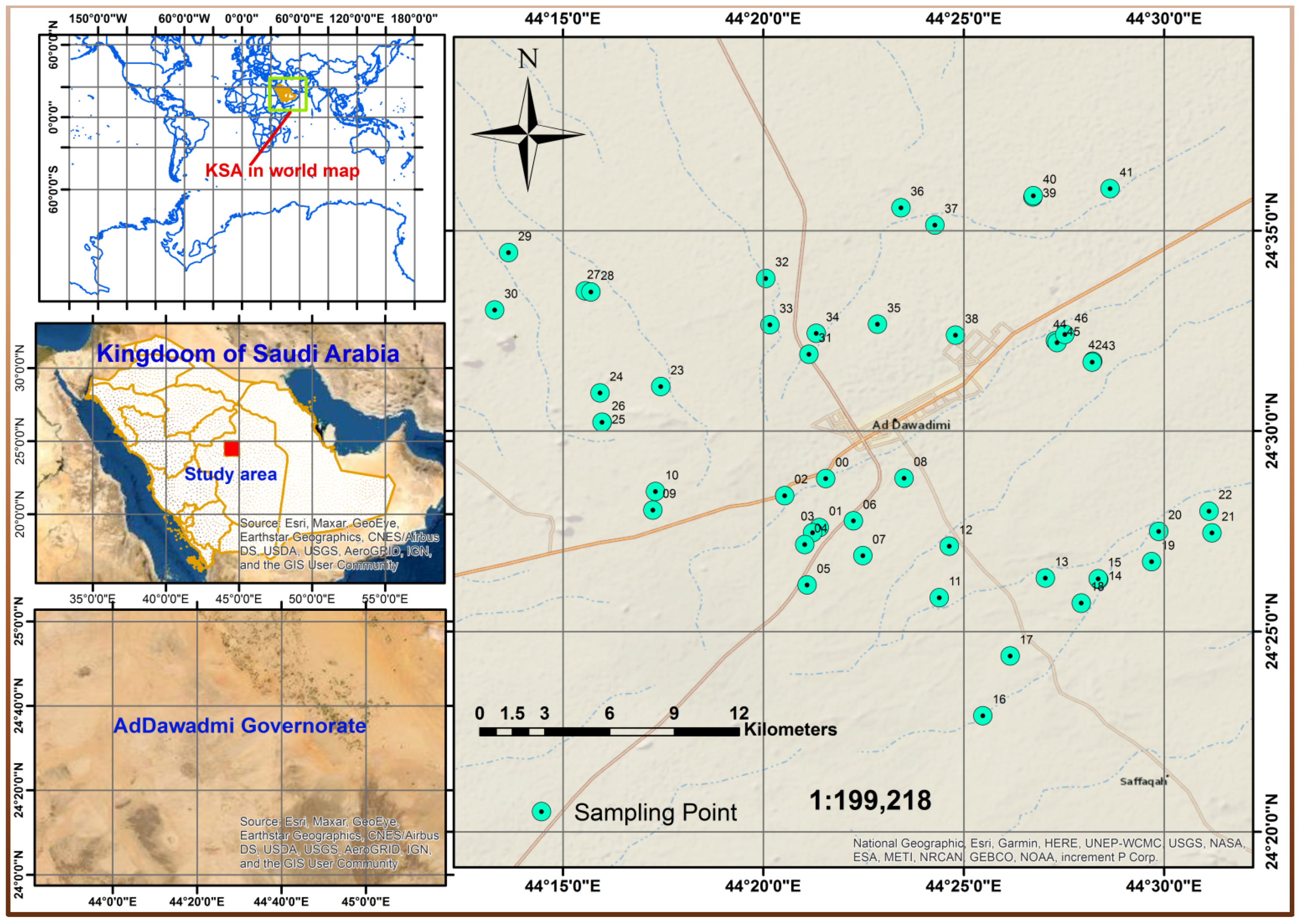
2.1. Description of the Study Area
2.2. Sampling and Preservation
2.3. Analyses and Procedures
2.3.1. In-Field Parameters
2.3.2. Hydrochemical Characterization
- a.
- Nitrate and Ammonium
- b.
- Dissolved Organic Carbon (DOC)
- c.
- Coliform detection
- d.
- Trace Elements Analysis
2.4. Geospatial and Geostatistical Analyses
3. Results and Discussion
3.1. Physicochemical and Microbiological, Properties
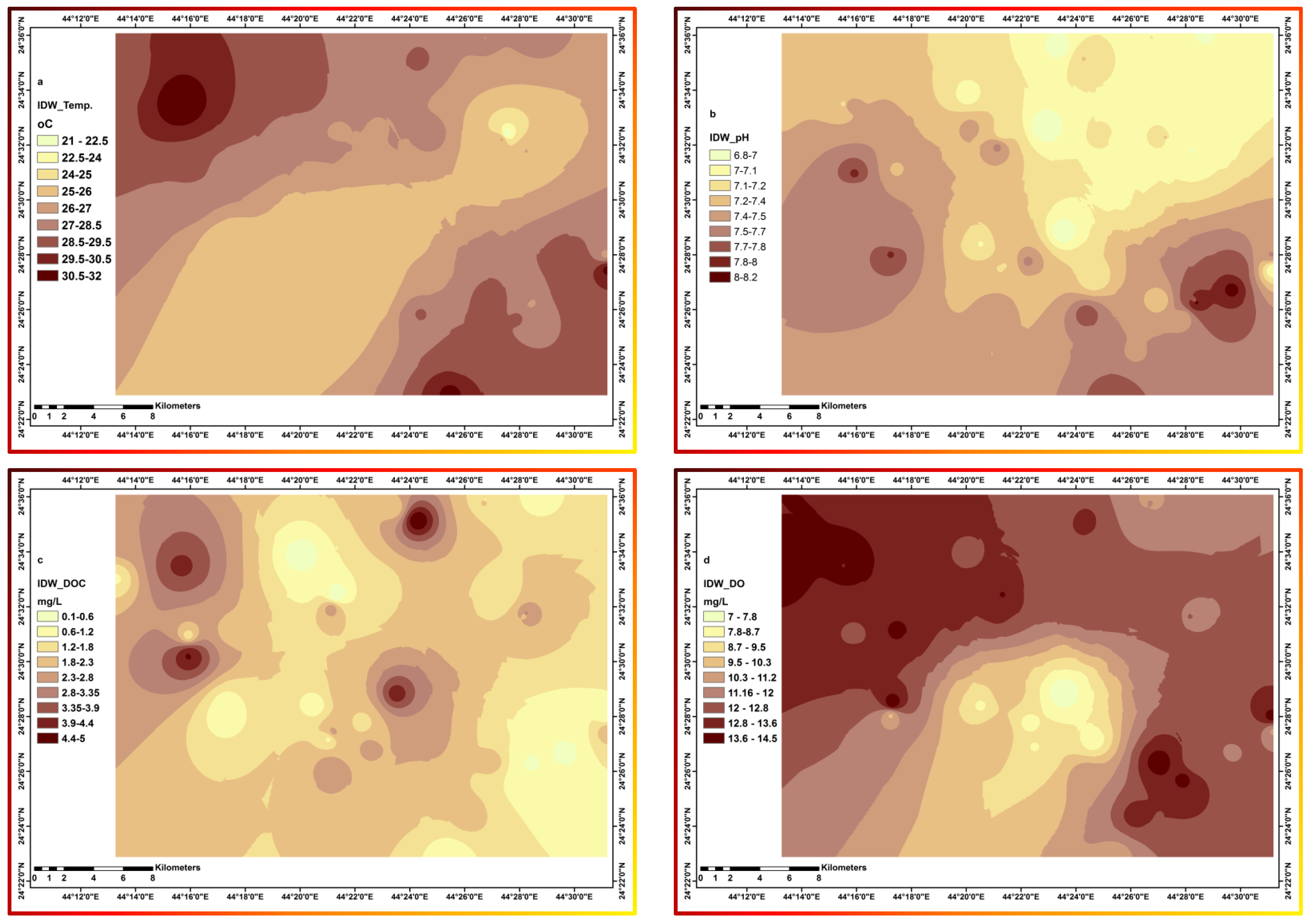
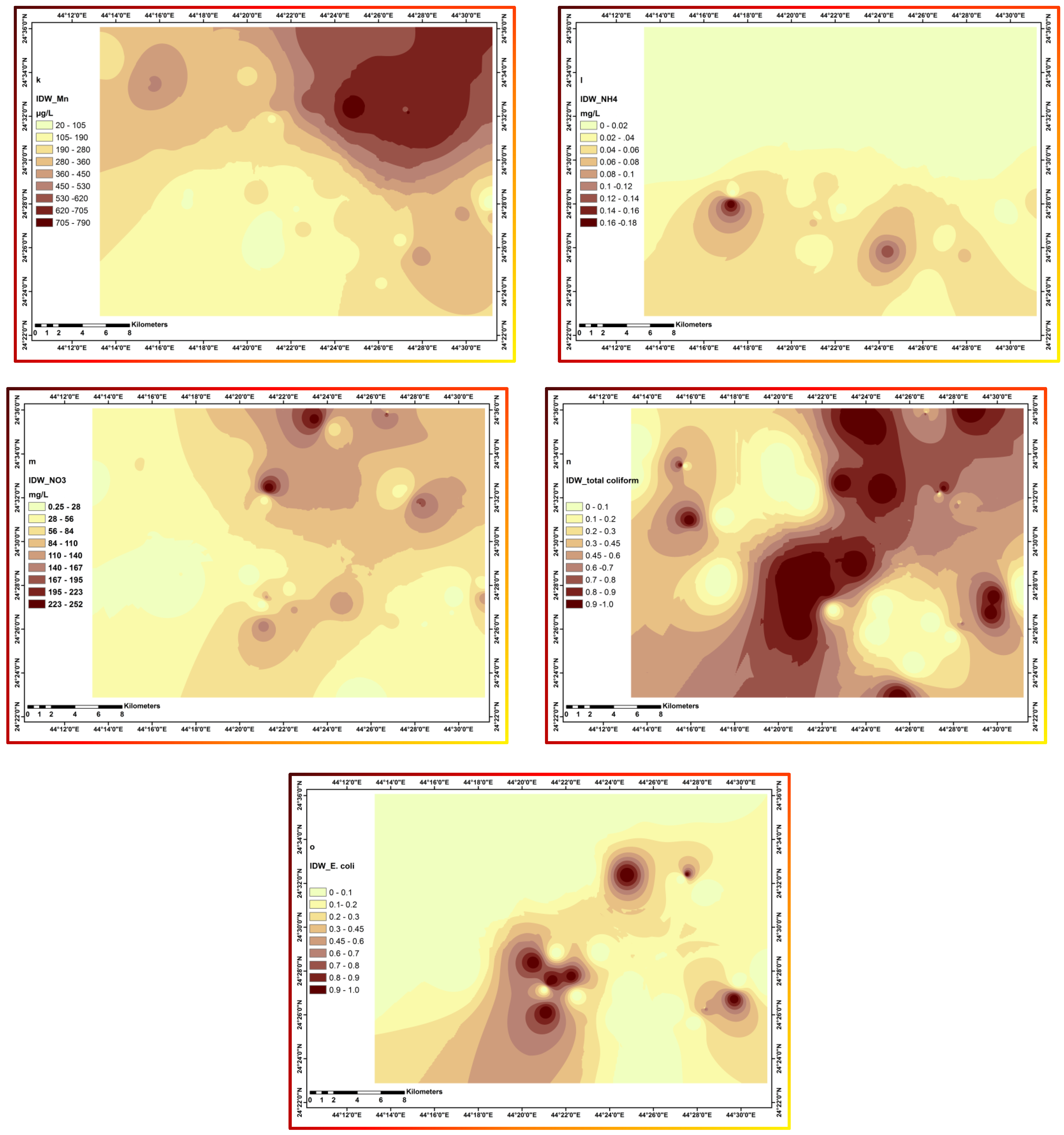
3.2. Spatial Distribution of the Measured Parameters
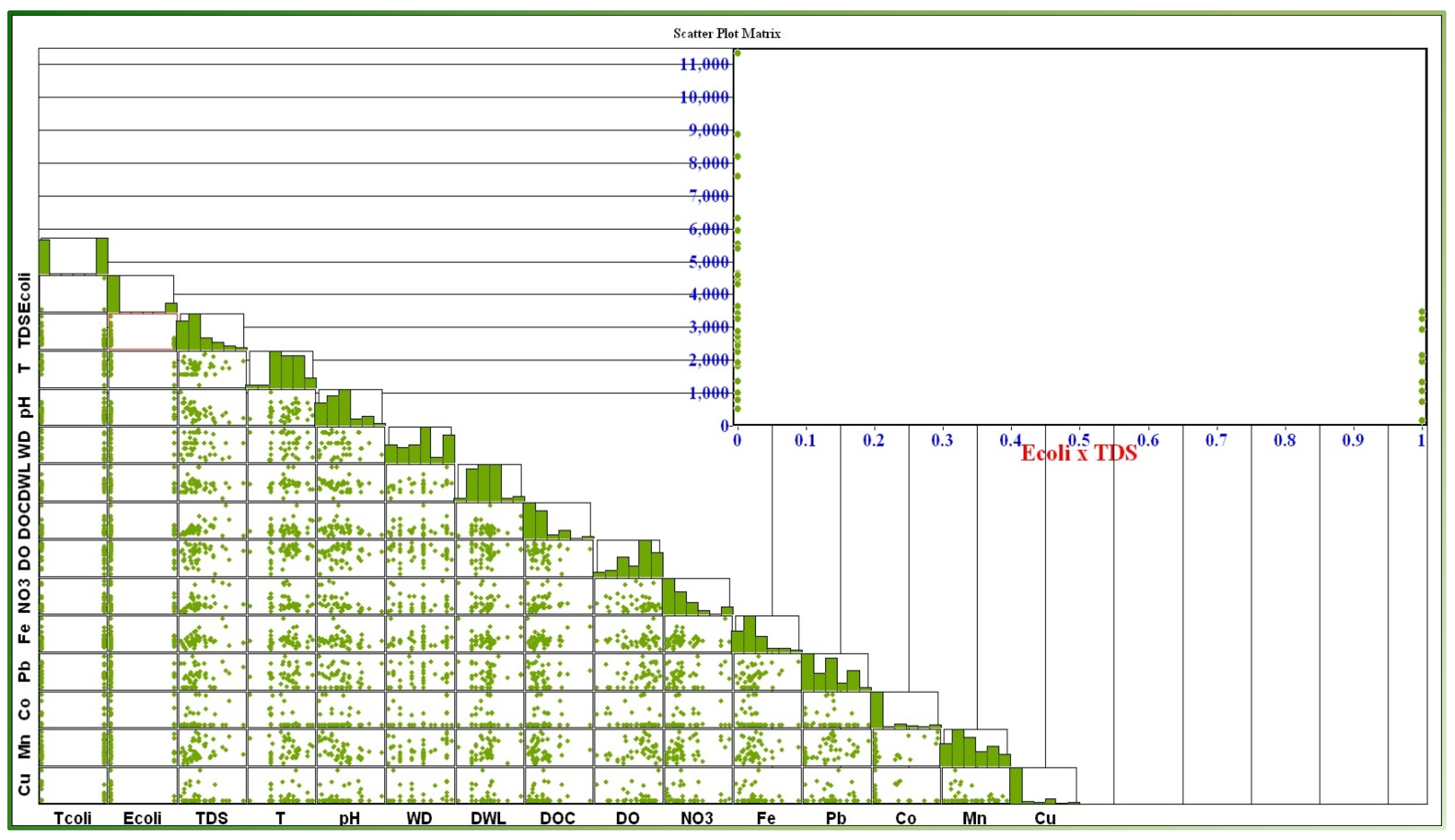
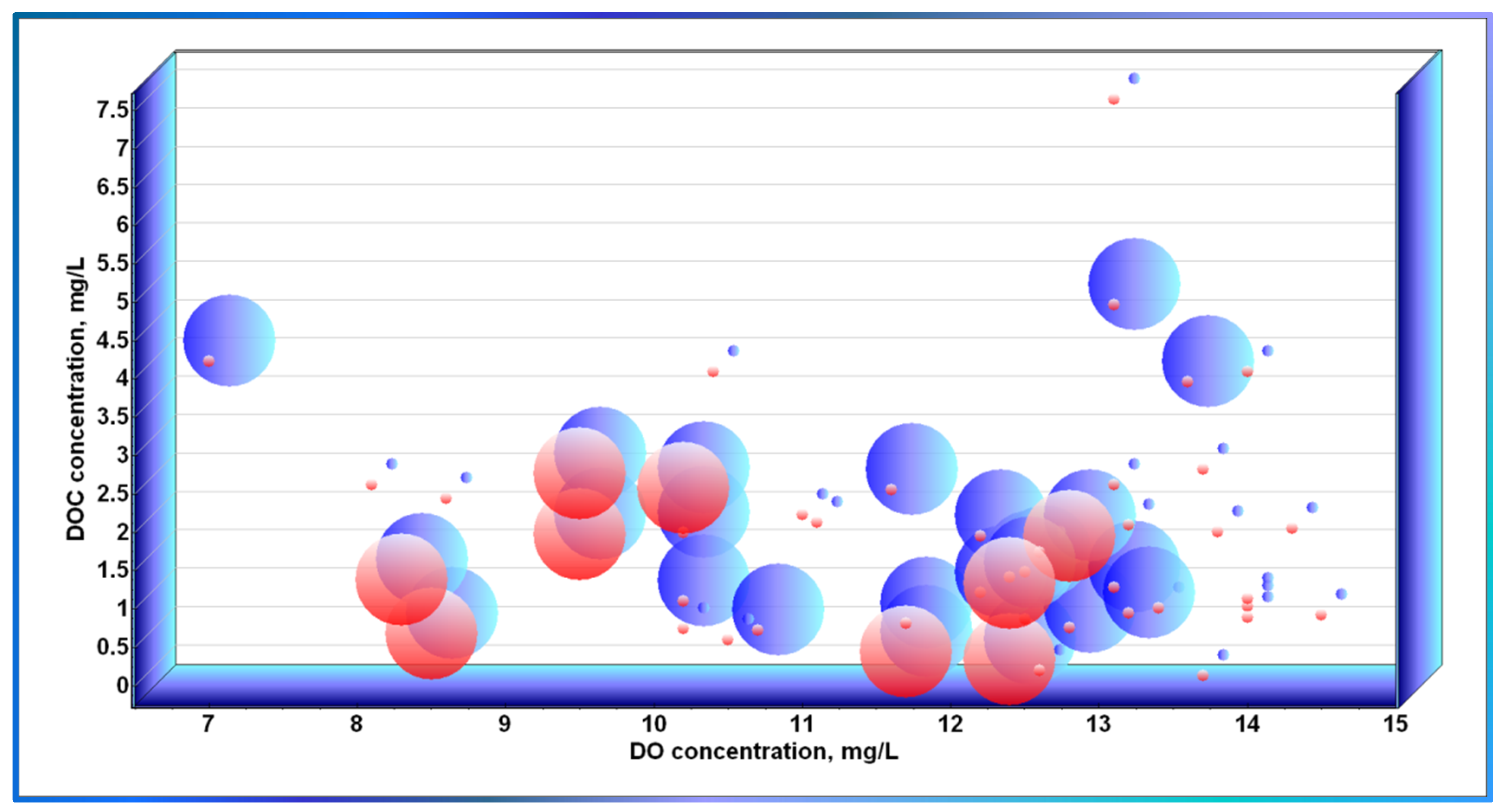
3.3. Interactions among the Interplaying Factors
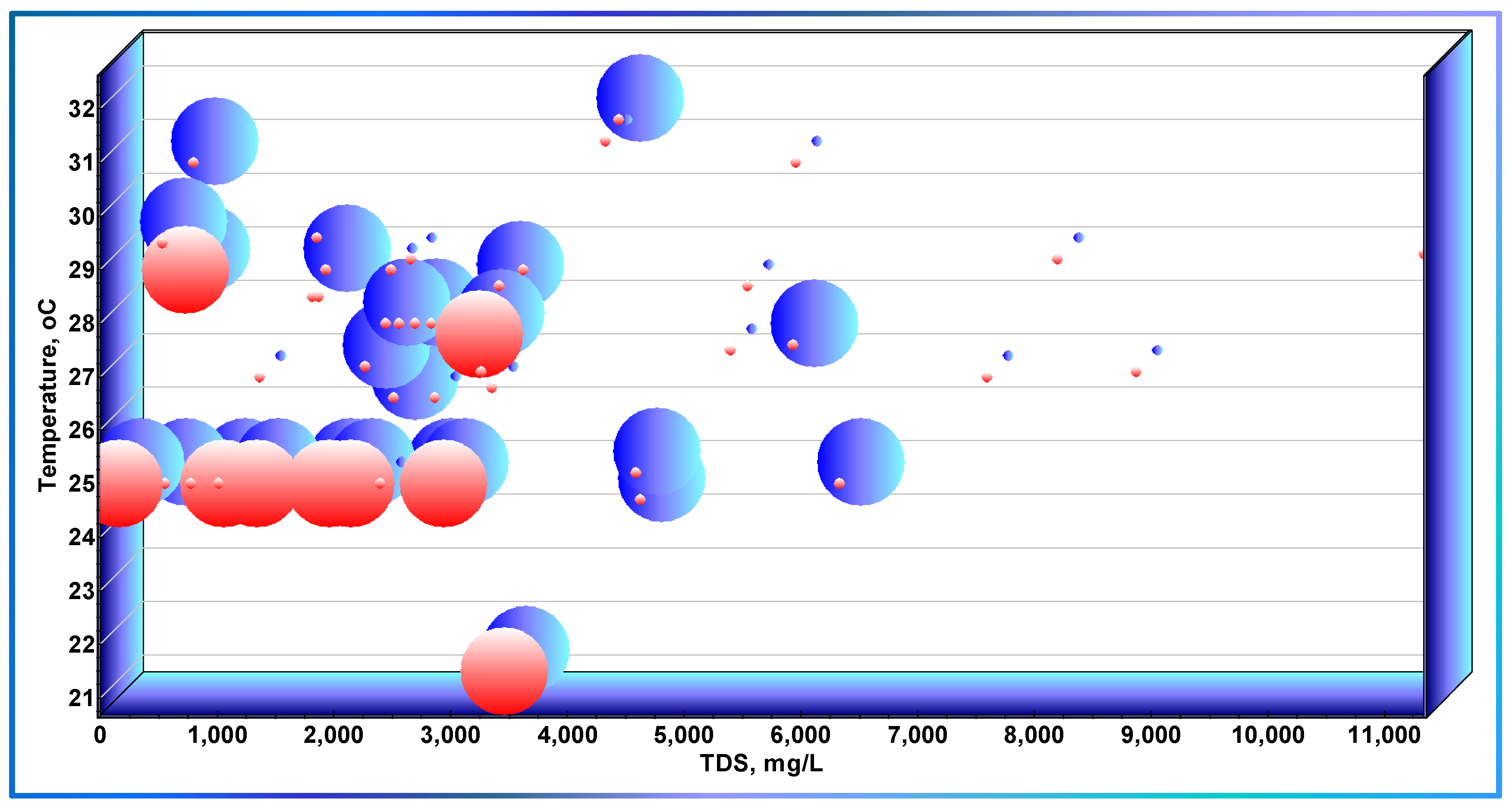
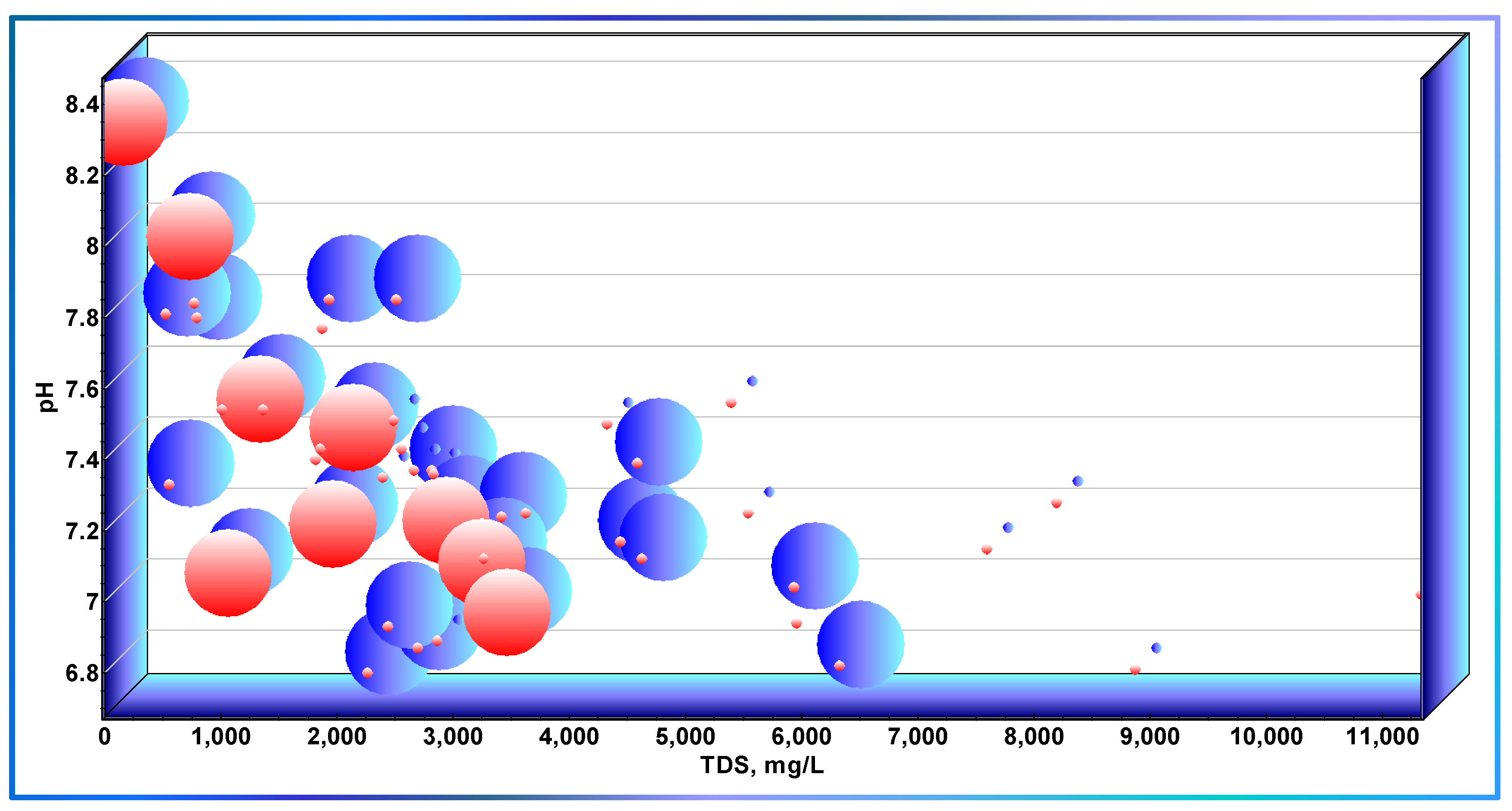
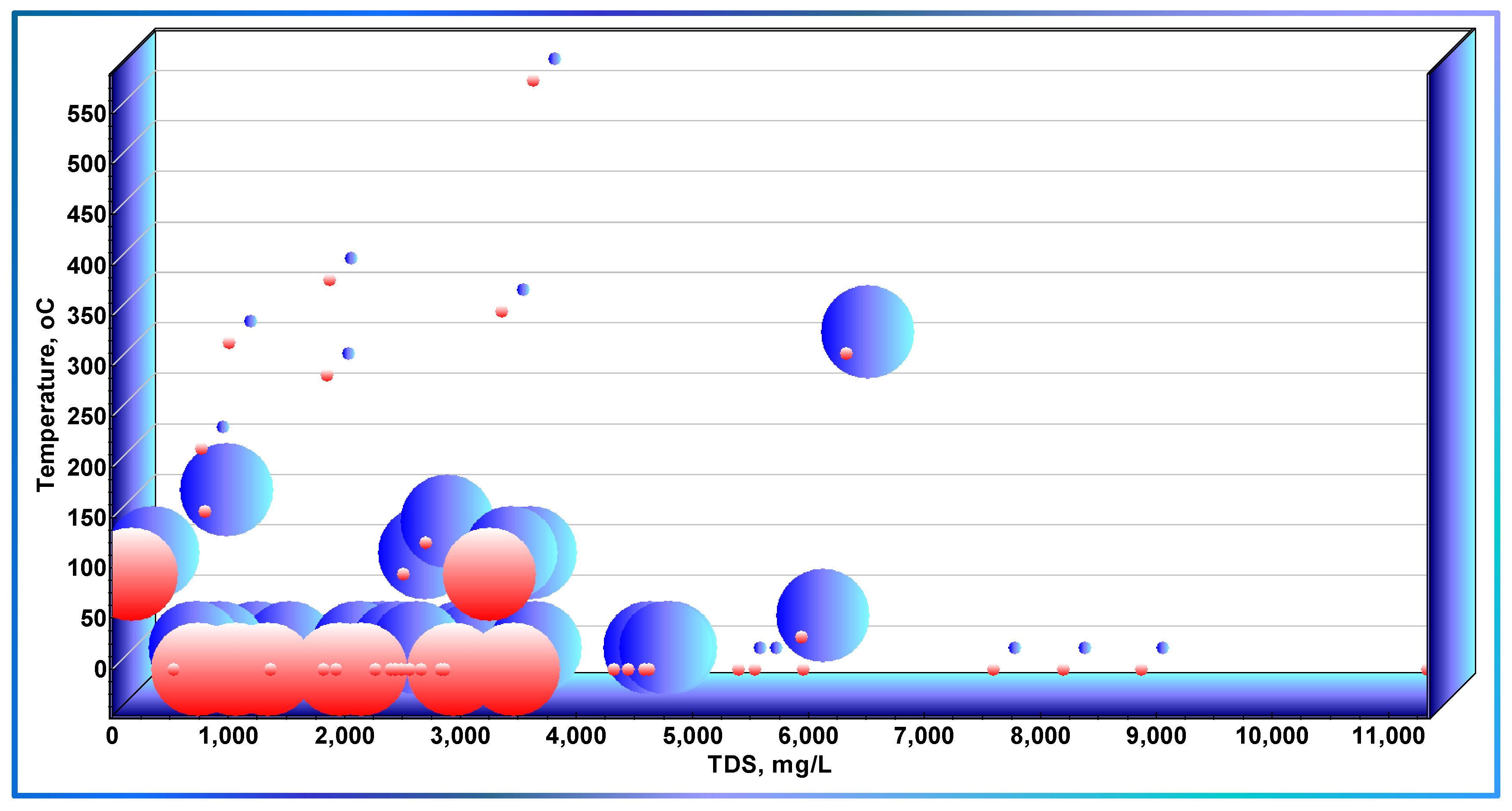
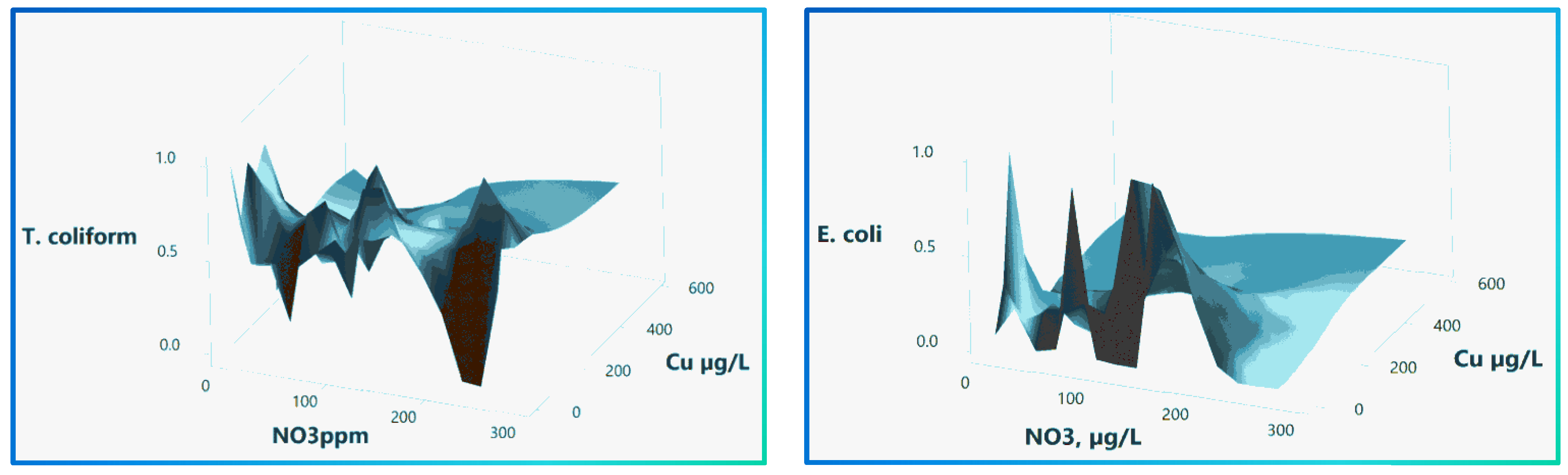
3.4. Synergistic Effects
3.5. Spearman Rho Correlation Analysis
4. Conclusions
- E. coli has higher sensitivity and less tolerability than TC towards the adversely influencing factors.
- Nitrate, DOC, and DO showed to be inversely distributed concerning the occurrence of fecal bacteria. Their quasi-random distribution may counteract the validity of their usage as coliforms surrogates.
- TDS exhibited a purification effect at ≈ 3500 mg/L and ≈ 6000 mg/L for E. coli and TC, respectively.
- The copper concentration effect was similar to TDS at 150 and 300 µg/L thresholds for E. coli and TC, respectively.
- The occurrence of FB in deep boreholes (30–52 m) with approximately no precipitation during the last five years challenges the sole water source that significantly threatens the region’s public health.
- Integrating various types of analyses was found to be powerful, as it helped constrain and provide multiple lines of evidence for the concluded remarks.
- A statistical Spearman’s rho correlation analysis yielded no consistent results with other methods due to the absence of the linear relationship that the test seeks.
Author Contributions
Funding
Institutional Review Board Statement
Informed Consent Statement
Data Availability Statement
Conflicts of Interest
References
- Jha, M.K.; Shekhar, A.; Jenifer, M.A. Assessing Groundwater Quality for Drinking Water Supply Using Hybrid Fuzzy-GIS-Based Water Quality Index. Water Res. 2020, 179, 115867. [Google Scholar] [CrossRef] [PubMed]
- Qu, S.; Shi, Z.; Liang, X.; Wang, G.; Han, J. Multiple Factors Control Groundwater Chemistry and Quality of Multi-Layer Groundwater System in Northwest China Coalfield—Using Self-Organizing Maps (SOM). J. Geochem. Explor. 2021, 227, 106795. [Google Scholar] [CrossRef]
- Dehnavi, A.; Sarikhani, R.; Nagaraju, D. Hydro Geochemical and Rock Water Interaction Studies in East of Kurdistan, NW of Iran. Int. J. Environ. Sci. Res. 2011, 1, 16–22. [Google Scholar]
- Subramani, T.; Rajmohan, N.; Elango, L. Groundwater Geochemistry and Identification of Hydrogeochemical Processes in a Hard Rock Region, Southern India. Environ. Monit. Assess. 2010, 162, 123–137. [Google Scholar] [CrossRef] [PubMed]
- Kumar, P.; Mahajan, A.K.; Kumar, A. Groundwater Geochemical Facie: Implications of Rock-Water Interaction at the Chamba City (HP), Northwest Himalaya, India. Environ. Sci. Pollut. Res. 2019, 27, 9012–9026. [Google Scholar] [CrossRef]
- Su, Y.-H.; Feng, Q.; Zhu, G.-F.; Si, J.-H.; Zhang, Y.-W. Identification and Evolution of Groundwater Chemistry in the Ejin Sub-Basin of the Heihe River, Northwest China. Pedosphere 2007, 17, 331–342. [Google Scholar] [CrossRef]
- Lotfi, S.; Chakit, M.; Najy, M.; Talbi, F.Z.; Benchahid, A.; El Kharrim, K.; Belghyti, D. Assessment of Microbiological Quality of Groundwater in the Saïs Plain (Morocco). Egypt. J. Aquat. Biol. Fish. 2020, 24, 509–524. [Google Scholar] [CrossRef] [Green Version]
- Xin, J.; Wang, Y.; Shen, Z.; Liu, Y.; Wang, H.; Zheng, X. Critical Review of Measures and Decision Support Tools for Groundwater Nitrate Management: A Surface-to-Groundwater Profile Perspective. J. Hydrol. 2021, 598, 126386. [Google Scholar] [CrossRef]
- Chen, H.; Teng, Y.; Lu, S.; Wang, Y.; Wu, J.; Wang, J. Source Apportionment and Health Risk Assessment of Trace Metals in Surface Soils of Beijing Metropolitan, China. Chemosphere 2016, 144, 1002–1011. [Google Scholar] [CrossRef]
- US EPA Seminar Publication. Groundwater Contamination; Wellhead Protection:A Guide for Small Communities. Chapter 3. EPA/625/R-93/002; Available online: chrome-extension://efaidnbmnnnibpcajpcglclefindmkaj/https://www.epa.gov/sites/default/files/2015-08/documents/mgwc-gwc1.pdf (accessed on 9 October 2022).
- Griesel, M.; Jagals, P. Faecal Indicator Organisms in the Renoster Spruit System of the Modder-Riet River Catchment and Implications for Human Users of the Water. Water SA 2002, 28, 227–234. [Google Scholar] [CrossRef] [Green Version]
- Aram, S.A.; Saalidong, B.M.; Lartey, P.O. Comparative Assessment of the Relationship between Coliform Bacteria and Water Geochemistry in Surface and Ground Water Systems. PLoS ONE 2021, 16, e0257715. [Google Scholar] [CrossRef] [PubMed]
- Ramírez-Castillo, F.Y.; Loera-Muro, A.; Jacques, M.; Garneau, P.; Avelar-González, F.J.; Harel, J.; Guerrero-Barrera, A.L. Waterborne Pathogens: Detection Methods and Challenges. Pathogens 2015, 4, 307–334. [Google Scholar] [CrossRef] [PubMed]
- Dzwairo, B.; Hoko, Z.; Love, D.; Guzha, E. Assessment of the Impacts of Pit Latrines on Groundwater Quality in Rural Areas: A Case Study from Marondera District, Zimbabwe. Phys. Chem. 2006, 31, 779–788. [Google Scholar] [CrossRef]
- Cabral, J.P.S.; Center Water Microbiology. Bacterial Pathogens and Water. Int. J. Environ. Res. Public Health 2010, 7, 3657–3703. [Google Scholar] [CrossRef]
- WHO. Guidelines for Drinking-Water Quality, 4th ed.; WHO: Geneva, Switzerland, 2017. [Google Scholar]
- Albaggar, A. Saudi Journal of Biological Sciences Investigation of Some Physical, Chemical, and Bacteriological Parameters of Water Quality in Some Dams in Albaha Region, Saudi Arabia. Saudi J. Biol. Sci. 2021, 28, 4605–4612. [Google Scholar] [CrossRef]
- Seo, M.; Lee, H.; Kim, Y. Relationship between Coliform Bacteria and Water Quality Factors at Weir Stations in the Nakdong River, South Korea. Water 2019, 11, 1171. [Google Scholar] [CrossRef] [Green Version]
- Bryan, S.W.S. Coliform Bacteria. Available online: https://extension.psu.edu/coliform-bacteria (accessed on 28 October 2022).
- Neill, M. Microbiological Indices for Total Coliform and E. Coli Bacteria in Estuarine Waters. Mar. Pollut. Bull. 2004, 49, 752–760. [Google Scholar] [CrossRef]
- Armah, F.A. Relationship Between Coliform Bacteria and Water Chemistry in Groundwater Within Gold Mining Environments in Ghana. Water Qual. Expo. Health 2014, 5, 183–195. [Google Scholar] [CrossRef]
- GSO 149/2014; Unbottled Drinking Water. GCC Standardization Organization (GSO): Riyadh, Saudi Arabia, 2014.
- Herschy, R.W. Water Quality for Drinking: WHO Guidelines. In Encyclopedia of Lakes and Reservoirs; Encyclopedia of Earth Sciences Series; Bengtsson, L., Herschy, R.W., Fairbridge, R.W., Eds.; Springer: Dordrecht, The Netherlands, 2012. [Google Scholar] [CrossRef]
- Huang, X.-Y.; Zhang, D.; Zhao, Z.-Q.; Liu, Y.-T.; Meng, H.-Q.; Zou, S.; Ma, B.-J.; Feng, Q.-Y. Determining Hydrogeological and Anthropogenic Controls on N Pollution in Groundwater beneath Piedmont Alluvial Fans Using Multi-Isotope Data. J. Geochem. Explor. 2021, 229, 106844. [Google Scholar] [CrossRef]
- Macler, B.A.; Merkle, J.C. Current Knowledge on Groundwater Microbial Pathogens and Their Control. Hydrogeol. J. 2000, 8, 29–40. [Google Scholar] [CrossRef]
- Poulin, C.; Peletz, R.; Ercumen, A.; Pickering, A.J.; Marshall, K.; Boehm, A.B.; Khush, R.; Delaire, C. What Environmental Factors in Fl Uence the Concentration of Fecal Indicator Bacteria in Groundwater? Insights from Explanatory Modeling in Uganda and Bangladesh. Environ. Sci. Technol. 2020, 54, 13566–13578. [Google Scholar] [CrossRef]
- Subba Rao, N.; Marghade, D.; Dinakar, A.; Chandana, I.; Sunitha, B.; Ravindra, B.; Balaji, T. Geochemical Characteristics and Controlling Factors of Chemical Composition of Groundwater in a Part of Guntur District, Andhra Pradesh, India. Environ. Earth Sci. 2017, 76, 747. [Google Scholar] [CrossRef]
- Barba, C.; Folch, A.; Sanchez-vila, X.; Martínez-alonso, M.; Gaju, N. Are Dominant Microbial Sub-Surface Communities a Ff Ected by Water Quality and Soil Characteristics? J. Environ. Manag. 2019, 237, 332–343. [Google Scholar] [CrossRef] [PubMed]
- Tropea, E.; Hynds, P.; Mcdermott, K.; Brown, R.S.; Majury, A. Environmental Adaptation of E. Coli within Private Groundwater Sources in Southeastern Ontario: Implications for Groundwater Quality Monitoring and Human Health. Environ. Pollut. 2021, 285, 117263. [Google Scholar] [CrossRef]
- Abed, S.M.; Alaraji, K.H.Y.; Essa, R.H. Assessment of the Biological and Physiochemical Properties of Groundwater in Al-Muthanna Province, Iraq. Eur. Asian J. Biosci. 2020, 5432, 5425–5432. [Google Scholar]
- Murray, R.T.; Rosenberg Goldstein, R.E.; Maring, E.F.; Pee, D.G.; Aspinwall, K.; Wilson, S.M.; Sapkota, A.R. Prevalence of Microbiological and Chemical Contaminants in Private Drinking Water Wells in Maryland, Usa. Int. J. Environ. Res. Public Health 2018, 15, 1686. [Google Scholar] [CrossRef] [Green Version]
- Thériault, A.; Duchesne, S. Quantifying the Fecal Coliform Loads in Urban Watersheds by Hydrologic/Hydraulic Modeling: Case Study of the Beauport River Watershed in Quebec. Water 2015, 7, 615–633. [Google Scholar] [CrossRef] [Green Version]
- Gorems, W.; Sisay, A. Fecal Coliform Bactria Extent and Distribution Assessment in Lake Hawassa Fecal Coliform Bactria Extent and Distribution Assessment in Lake Hawassa Watershed. J. Med. Physiol. Biophys. 2018, 50, 25–33. [Google Scholar]
- Akpataku, K.V.; Gnazou, M.D.T.; Yawo, T.; Nomesi, A. Physicochemical and Microbiological Quality of Shallow Groundwater in Lomé, Togo. J. Geosci. Environ. Prot. 2020, 8, 162–179. [Google Scholar] [CrossRef]
- Howard, G.; Pedley, S.; Barrett, M.; Nalubega, M.; Johal, K. Risk Factors Contributing to Microbiological Contamination of Shallow Groundwater in Kampala, Uganda. Water Res. 2003, 37, 3421–3429. [Google Scholar] [CrossRef]
- Dwyer, J.O.; Chique, C.; Weatherill, J.; Hynds, P. Impact of the 2018 European Drought on Microbial Groundwater Quality in Private Domestic Wells: A Case Study from a Temperate Maritime Climate. J. Hydrol. 2021, 601, 126669. [Google Scholar] [CrossRef]
- Mandel, S.; Shiftam, Z.L.; Hamill, L.; Bell, F.G.; Ingraham, N.L.; Caldwell, E.A.; Verhagen, B.T.; Finkelman, R.B.; Orem, W.H.; Plumlee, G.S.; et al. Sustainability of Morocco’s Groundwater Resources in Response to Natural and Anthropogenic Forces. J. Hydrol. 2021, 603, 106795. [Google Scholar] [CrossRef]
- Ravindra, K.; Thind, P.S.; Mor, S.; Singh, T.; Mor, S. Evaluation of Groundwater Contamination in Chandigarh: Source Identification and Health Risk Assessment. Environ. Pollut. 2019, 255, 113062. [Google Scholar] [CrossRef]
- Chique, C.; Hynds, P.; Burke, L.P.; Morris, D.; Ryan, M.P.; Dwyer, J.O. Contamination of Domestic Groundwater Systems by Verotoxigenic Escherichia Coli (VTEC), 2003–2019: A Global Scoping Review. Water Res. 2021, 188, 116496. [Google Scholar] [CrossRef]
- Ferrerons, G.M.; Folch, A.; Masó, G.; Sanchez, S.; Sanchez-Vila, X. What are the main factors influencing the presence of faecal bacteria pollution in groundwater systems in developing countries? J. Contam. Hydrol. 2019, 228, 103556. [Google Scholar] [CrossRef]
- Ferrer, N.; Folch, A.; Lane, M.; Olago, D.; Odida, J.; Custodio, E. Science of the Total Environment Groundwater Hydrodynamics of an Eastern Africa Coastal Aquifer, in- Cluding La Niña 2016–2017 Drought. Sci. Total Environ. 2019, 661, 575–597. [Google Scholar] [CrossRef]
- Van Elsas, J.D.; Semenov, A.V.; Costa, R.; Trevors, J.T. Survival of Escherichia Coli in the Environment: Fundamental and Public Health Aspects. ISME J. 2011, 5, 173–183. [Google Scholar] [CrossRef] [Green Version]
- Yang, Y.; Wu, Y.; Lu, Y.; Shi, M.; Chen, W. Microorganisms and Their Metabolic Activities Affect Seepage through Porous Media in Groundwater Artificial Recharge Systems: A Review. J. Hydrol. 2021, 598, 126256. [Google Scholar] [CrossRef]
- Osei, F.B.; Boamah, V.E.; Agyare, C.; Abaidoo, R.C. Physicochemical Properties and Microbial Quality of Water Used in Selected Poultry Farms in the Ashanti Region of Ghana. Open Microbiol. J. 2019, 13, 121–127. [Google Scholar] [CrossRef] [Green Version]
- Kadyampakeni, D.; Appoh, R.; Barron, J.; Boakye-Acheampong, E. Analysis of Water Quality of Selected Irrigation Water Sources in Northern Ghana. Water Sci. Technol. Water Supply 2018, 18, 1308–1317. [Google Scholar] [CrossRef]
- Jin, D.; Ligaray, M.; Kim, M.; Kim, G.; Lee, G.; Pachepsky, Y.A.; Cha, D.; Hwa, K. Science of the Total Environment Evaluating the in Fl Uence of Climate Change on the Fate and Transport of Fecal Coliform Bacteria Using the Modi Fi Ed SWAT Model. Sci. Total Environ. 2019, 658, 753–762. [Google Scholar] [CrossRef]
- Reynolds, L.J.; Martin, N.A.; Sala-comorera, L.; Callanan, K.; Doyle, P.; Leary, C.O.; Buggy, P.; Nolan, T.M.; Hare, G.M.P.O.; Sullivan, J.J.O.; et al. Identifying Sources of Faecal Contamination in a Small Urban Stream Catchment: A Multiparametric Approach. Front. Microbiol. 2021, 12, 661954. [Google Scholar] [CrossRef]
- Alsalah, D.; Al-Jassim, N.; Timraz, K.; Hong, P.Y. Assessing the Groundwater Quality at a Saudi Arabian Agricultural Site and the Occurrence of Opportunistic Pathogens on Irrigated Food Produce. Int. J. Environ. Res. Public Health 2015, 12, 12391–12411. [Google Scholar] [CrossRef] [Green Version]
- Ferguson, C.; Kay, D. Transport of Microbial Pollution in Catchment Systems. In Animal Waste, Water Quality and Human Health; Al Dufour, J.B., Gannon, R.B., Eds.; IWA Publishing, London, UK, 2012; ISBN 9781780401232. [Google Scholar]
- Ekarini, F.D.; Rafsanjani, S.; Rahmawati, S.; Asmara, A.A. Groundwater Mapping of Total Coliform Contamination in Sleman, Yogyakarta, Indonesia Groundwater Mapping of Total Coliform Contamination in Sleman, Yogyakarta, Indonesia. IOP Conf. Ser. Earth Environ. Sci. 2021, 933, 012047. [Google Scholar] [CrossRef]
- Ouedraogo, I.; Defourny, P.; Vanclooster, M. Mapping the Groundwater Vulnerability for Pollution at the Pan African Scale. Sci. Total Environ. 2016, 544, 939–953. [Google Scholar] [CrossRef]
- Carlson, H.K.; Price, M.N.; Callaghan, M.; Aaring, A.; Chakraborty, R.; Kuehl, J.V.; Arkin, A.P.; Deutschbauer, A.M. The Selective Pressures on the Microbial Community in a Metal- Contaminated Aquifer. ISME J. 2018, 13, 937–949. [Google Scholar] [CrossRef] [Green Version]
- Carneiro, M.T.; Wasserman, J.C. Critical Evaluation of the Factors Affecting Escherichia Coli Environmental Decay for Outfall Plume Models. Rev. Ambient. e Agua 2014, 9, 445–458. [Google Scholar] [CrossRef]
- Xue, F.; Tang, J.; Dong, Z.; Shen, D.; Liu, H.; Zhang, X.; Holden, N.M. Tempo-Spatial Controls of Total Coliform and E. Coli Contamination in a Subtropical Hilly Agricultural Catchment. Agric. Water Manag. 2018, 200, 10–18. [Google Scholar] [CrossRef]
- Enuneku, A.A.; Abhulimen, P.I.; Omoregie, P.; Osaro, C.; Okpara, B.; Imoobe, T.O.; Ezemonye, L.I. Heliyon Interactions of Trace Metals with Bacteria and Fungi in Selected Agricultural Soils of Egbema Kingdom, Warri North, Delta State, Nigeria. Heliyon 2020, 6, e04477. [Google Scholar] [CrossRef]
- Ferreira, M.; Vaz-moreira, I.; Gonzalez-pajuelo, M.; Nunes, O.C.; Manaia, M. Antimicrobial Resistance Patterns in Enterobacteriaceae Isolated from an Urban Wastewater Treatment Plant. FEMS Microbiol. Ecol. 2007, 60, 166–176. [Google Scholar] [CrossRef]
- Ntube, N.S.; Nyangang, A.J.; Agbor, M.-E.N.; Ayuk, A.R. Trace Element Evaluation of Groundwater in Douala, Cameroon. OALib 2022, 9, 1–21. [Google Scholar] [CrossRef]
- Rajapaksha, R.M.; Tobor-Kapłon, M.A.; Bååth, E. Metal Toxicity Affects Fungal and Bacterial Activities in Soil Differently. Appl. Environ. Microbiol. 2004, 70, 2966–2973. [Google Scholar] [CrossRef]
- AdDawadmi_Gover. Available online: https://ar.wikipedia.org/wiki/محافظة_الدوادمي (accessed on 12 March 2022).
- SSYB Annual Yearbook|General Authority for Statistics. 24 October 2010. Available online: https://www.stats.gov.sa/en/46 (accessed on 24 October 2022).
- EL-DIDY, S. Evaluation of The Proposed Drainage Network for Lowering the Groundwater Levels in Al-Dawadmi Town. J. King Abdulaziz Univ. Environ. Arid L. Agric. Sci. 1997, 8, 111–123. [Google Scholar] [CrossRef]
- Al-Zaidi, A.A.; Elhag, E.A.; Al-Otaibi, S.H.; Baig, M.B. Negative Effects of Pesticides on the Environment and the Farmers Awareness in Saudi Arabia: A Case Study. J. Anim. Plant Sci. 2011, 21, 605–611. [Google Scholar]
- Al Shanti, A. The Geology and Mineralization of the AdDawadmi District of Saudi Arabia; Imperial College London: London, UK, 1973. [Google Scholar]
- El-Sawy, E.K.; Eldougdoug, A.; Gobashy, M. Geological and Geophysical Investigations to Delineate the Subsurface Extension and the Geological Setting of Al Ji’lani Layered Intrusion and Its Mineralization Potentiality, Ad Dawadimi District, Kingdom of Saudi Arabia. Arab. J. Geosci. 2018, 11, 32. [Google Scholar] [CrossRef]
- Johnson, P.R. Explanatory Notes to the Map of Proterozoic Geology of Western Saudi Arabia; Saudi Geological Survey Technical Report SGS-TR-2006-4; Saudi Geological Survey: Jeddah, Saudi Arabia, 2006; 62 p. [Google Scholar]
- Timeanddate Climate and Weather Averages in Ad Dawadmi, Saudi Arabia. Available online: https://www.timeanddate.com/weather/saudi-arabia/dawadmi/climate (accessed on 12 March 2022).
- Silva, M.I.; Gonçalves, A.M.L.; Lopes, W.A.; Lima, M.T.V.; Costa, C.T.F.; Paris, M.; Firmino, P.R.A.; De Paula Filho, F.J. Assessment of Groundwater Quality in a Brazilian Semiarid Basin Using an Integration of GIS, Water Quality Index and Multivariate Statistical Techniques. J. Hydrol. 2021, 598, 126346. [Google Scholar] [CrossRef]
- Quevauviller, P.; Thompson, K.C. Analytical Methods for Drinking Water; Wiley: Hoboken, NJ, USA, 2005; ISBN 9780470094938. [Google Scholar]
- DPIR. Methodology for the Sampling of Surface Water. North. Territ. Gov. 1998, 11, 1–11. [Google Scholar]
- UGSS. National Field Manual for the Collection of Water-Quality Data. U.S. Geological Survey Techniques of Water-Resources Investigations; Book 9; USGS: Reston, VA, USA, 2015. [Google Scholar]
- Middleton, K.R. A New Procedure for Rapid Determination of Nitrate and a Study of the Preparation of the Phenol-Sulphonic Acid Reagent. J. Appl. Chem. 1958, 8, 505–509. [Google Scholar] [CrossRef]
- Ahmed, M.A.; Al Aly, I.M.; Bastaweesy, A.; Gomaa, H.E. Modified Low-Priced Ammonia Diffusion Method for the Analysis of Nitrogen Isotopic Composition of Ammonium and Nitrate in Different Water Matrices. Egypt. J. Radiat. Sci. Appl. 2006, 21, 257–281. [Google Scholar]
- Water Quality-HyServe. Available online: https://hyserve.com/en/solutions/water-quality/ (accessed on 28 October 2022).
- Feng, P.C.S.; Hartman, P.A. Fluorogenic Assays for Immediate Confirmation of Escherichia Coli. Appl. Environ. Microbiol. 1982, 43, 1320–1329. [Google Scholar] [CrossRef] [Green Version]
- Hansen, W.; Yourassowsky, E. Detection of β-Glucuronidase in Lactose-Fermenting Members of the Family Enterobacteriaceae and Its Presence in Bacterial Urine Cultures. J. Clin. Microbiol. 1984, 20, 1177–1179. [Google Scholar] [CrossRef] [PubMed] [Green Version]
- Ahmad, A.Y.; Al-Ghouti, M.A.; Khraisheh, M.; Zouari, N. Hydrogeochemical Characterization and Quality Evaluation of Groundwater Suitability for Domestic and Agricultural Uses in the State of Qatar. Groundw. Sustain. Dev. 2020, 11, 100467. [Google Scholar] [CrossRef]
- Komisarek, J. Groundwater chemistry and hydrogeochemical processes in a soil catena of the poznań Lakeland. J. Elem. 2017, 22, 681–695. [Google Scholar] [CrossRef]
- Mallick, J.; Singh, C.K.; AlMesfer, M.K.; Kumar, A.; Khan, R.A.; Islam, S.; Rahman, A. Hydro-Geochemical Assessment of Groundwater Quality in Aseer Region, Saudi Arabia. Water 2018, 10, 1847. [Google Scholar] [CrossRef] [Green Version]
- USEPA. National Primary Drinking Water Regulations|Ground Water and Drinking Water|US EPA. Available online: https://www.epa.gov/ground-water-and-drinking-water/national-primary-drinking-water-regulations#Inorganic (accessed on 23 February 2021).
- WHO. PH in Drinking-Water Revised Background Document for Development of WHO Guidelines for Drinking-Water Quality; WHO/SDE/WSH/07.01/1; WHO: Geneva, Switzerland, 2007. [Google Scholar]
- USEPA. National Primary Drinking Water Guidelines; Epa 816-F-09-004; USEPA: Washington, DC, USA, 2009; Volume 1, p. 7. [Google Scholar]
- Gulf Technical Regulation GSO5/DS, D. GCC Standardization Organization (GSO). Food Packag. Part 2 Plast. Package–Gen. RequirEments 2013, 2013, 83. [Google Scholar]
- How Water Activity and PH Synergize|METER Group. Available online: https://www.metergroup.com/en/meter-food/expertise-library/how-water-activity-and-ph-work-together-control-microbial-growth (accessed on 25 October 2022).
- Curtis, T.P.; Mara, D.D.; Silva, S.A. Influence of PH, Oxygen, and Humic Substances on Ability of Sunlight to Damage Fecal Coliforms in Waste Stabilization Pond Water. Appl. Environ. Microbiol. 1992, 58, 1335–1343. [Google Scholar] [CrossRef] [PubMed]
- Wahyuni, E.A. The Influence of PH Characteristics on The Occurance of Coliform Bacteria in Madura Strait. Procedia Environ. Sci. 2015, 23, 130–135. [Google Scholar] [CrossRef] [Green Version]
- Minitab Support System. The Anderson-Darling Statistic-Minitab. Available online: https://support.minitab.com/en-us/minitab/18/help-and-how-to/statistics/basic-statistics/supporting-topics/normality/the-anderson-darling-statistic/ (accessed on 17 March 2022).
- Minitab® 18 Support Overview of Boxplot-Minitab. Boxplot to Assess and Outliers for Each Group. Available online: https://support.minitab.com/en-us/minitab/20/help-and-how-to/graphs/boxplot/before-you-start/overview/#:~:text=Use (accessed on 24 October 2022).
- Marois-Fise, J.T.; Carabin, A.; Lavoie, A.; Dorea, C.C. Effects of Temperature and PH on Reduction of Bacteria in a Pointof- Use Drinking Water Treatment Product for Emergency Relief. Appl. Environ. Microbiol. 2013, 79, 2107–2109. [Google Scholar] [CrossRef] [Green Version]
- Hong, H.; Qiu, J.; Liang, Y. Environmental Factors Influencing the Distribution of Total and Fecal Coliform Bacteria in Six Water Storage Reservoirs in the Pearl River Delta Region, China. J. Environ. Sci. 2010, 22, 663–668. [Google Scholar] [CrossRef]
- Painchaud, J.; Therriault, J. Assessment of Salinity-Related Mortality of Freshwater Bacteria in the Saint Lawrence Estuary. Appl. Environ. Microbiol. 1995, 61, 205–208. [Google Scholar] [CrossRef] [Green Version]
- Griebler, C.; Lueders, T.; Mu, H.Z. Microbial Biodiversity in Groundwater Ecosystems. Freshw. Biol. 2009, 54, 649–677. [Google Scholar] [CrossRef]
- Kozhevin, P.A.; Verkhovtseva, N.V. Biological properties of soil and ground waters. Encycl. Life Support Syst. 2009, 30, 169. [Google Scholar]
- Yan, N.; Marschner, P.; Cao, W.; Zuo, C.; Qin, W. Influence of Salinity and Water Content on Soil Microorganisms. Int. Soil Water Conserv. Res. 2015, 3, 316–323. [Google Scholar] [CrossRef] [Green Version]
- Akhavan, S.; Ebrahimi, S.; Navabian, M.; Shabanpour, M.; Mojtahedi, A. Coli and Chloride Significance of Physicochemical Factors in the Transmission of Escherichia Coli and Chloride. Kerman Univ. Med. Sci. 2018, 5, 115–122. [Google Scholar] [CrossRef]
- Mamilov, A.; Dilly, O.M.; Mamilov, S.; Inubushi, K. Microbial Eco-Physiology of Degrading Aral Sea Wetlands: Consequences for C-Cycling. Soil Sci. Plant Nutr. 2004, 50, 839–842. [Google Scholar] [CrossRef] [Green Version]
- Willem, J.; Van Herwerden, M.; Schijven, J. Measuring and Modelling Straining of Escherichia Coli in Saturated Porous Media. J. Contam. Hydrol. 2007, 93, 236–254. [Google Scholar] [CrossRef]
- Dey, U.; Sarkar, S.; Duttagupta, S.; Bhattacharya, A. Influence of Hydrology and Sanitation on Groundwater Coliform Contamination in Some Parts of Western Bengal Basin: Implication to Safe Drinking Water. Front. Water 2022, 4, 1–15. [Google Scholar] [CrossRef]
- Minitab Support System. A Comparison of the Pearson and Spearman Correlation Methods-Minitab Express. Available online: https://support.minitab.com/en-us/minitab-express/1/help-and-how-to/modeling-statistics/regression/supporting-topics/basics/a-comparison-of-the-pearson-and-spearman-correlation-methods/ (accessed on 7 April 2022).


| Variable | Mean | SE Mean | sd | Coef. Var. | Min. | Q1 | Median | Q3 | Maximum | Range | IQR | Skewness | Kurtosis |
|---|---|---|---|---|---|---|---|---|---|---|---|---|---|
| Temp, °C | 27.32 | 0.32 | 2.17 | 7.94 | 21.50 | 25.00 | 27.50 | 29.00 | 31.80 | 10.30 | 4.00 | −0.10 | −0.13 |
| pH | 7.34 | 0.05 | 0.35 | 4.71 | 6.80 | 7.10 | 7.33 | 7.54 | 8.35 | 1.55 | 0.44 | 0.64 | 0.37 |
| TDS, mg/L | 3293.00 | 344.00 | 2359.00 | 71.65 | 161.00 | 1852.00 | 2696.00 | 4442.00 | 11,334.00 | 11,173.00 | 2590.00 | 1.39 | 2.18 |
| DO, mg/L | 11.88 | 0.28 | 1.88 | 15.85 | 7.00 | 10.40 | 12.40 | 13.20 | 14.50 | 7.50 | 2.80 | −0.78 | −0.22 |
| DOC, mg/L | 1.89 | 0.21 | 1.43 | 75.28 | 0.13 | 0.89 | 1.48 | 2.55 | 7.65 | 7.52 | 1.66 | 1.82 | 4.80 |
| TC | 0.51 | 0.07 | 0.51 | 98.95 | 0.00 | 0.00 | 1.00 | 1.00 | 1.00 | 1.00 | 1.00 | −0.04 | −2.09 |
| E. coli | 0.19 | 0.06 | 0.39 | 207.70 | 0.00 | 0.00 | 0.00 | 0.00 | 1.00 | 1.00 | 0.00 | 1.62 | 0.65 |
| NH4, mg/L | 0.024 | 0.005 | 0.04 | 150.10 | 0.00 | 0.00 | 0.007 | 0.04 | 0.18 | 0.18 | 0.04 | 2.44 | 7.49 |
| NO3, mg/L | 72.70 | 9.87 | 67.67 | 93.09 | 0.21 | 28.94 | 51.24 | 116.53 | 269.28 | 269.07 | 87.59 | 1.48 | 1.80 |
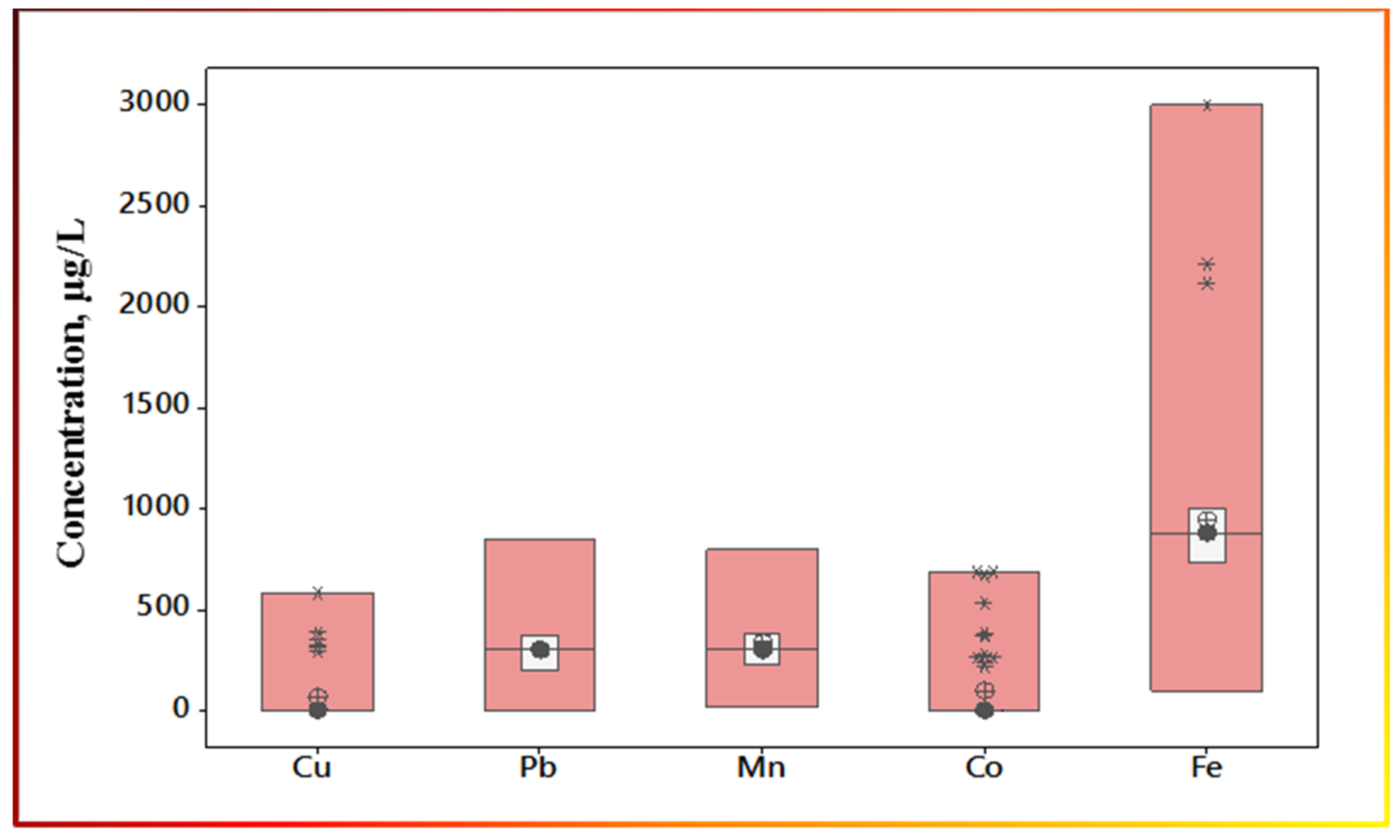
| Cu µg/L | 67.60 | 19.40 | 132.80 | 196.42 | 0.00 | 0.00 | 0.00 | 93.80 | 583.30 | 583.30 | 93.80 | 2.23 | 4.71 |
| Pb µg/L | 300.90 | 36.00 | 246.80 | 82.02 | 0.00 | 0.00 | 304.70 | 444.20 | 852.90 | 852.90 | 444.20 | 0.31 | −0.90 |
| Mn µg/L | 338.50 | 30.90 | 211.50 | 62.48 | 20.00 | 160.00 | 300.00 | 500.00 | 800.00 | 780.00 | 340.00 | 0.51 | −0.81 |
| Co µg/L | 98.90 | 29.00 | 198.50 | 200.74 | 0.00 | 0.00 | 0.00 | 41.10 | 684.90 | 684.90 | 41.10 | 2.03 | 3.12 |
| Fe µg/L | 942.90 | 81.20 | 556.70 | 59.04 | 100.00 | 543.50 | 880.00 | 1152.20 | 3000.00 | 2900.00 | 608.70 | 1.46 | 3.32 |
| WD, m BGL | 38.43 | 1.21 | 8.28 | 21.54 | 25.00 | 30.00 | 40.00 | 45.00 | 52.00 | 27.00 | 15.00 | 0.03 | −1.09 |
| Parameter | Total Coliform | E. coli | Parameter | Total Coliform | E. coli | Parameter | Total Coliform | E. coli |
|---|---|---|---|---|---|---|---|---|
| E.coli | 0.476 | Appearance | 0.082 | 0.034 | Cu µg/L | −0.038 | −0.133 | |
| p-Value | 0.001 | p-Value | 0.586 | 0.823 | p-Value | 0.800 | 0.374 | |
| Temp | −0.298 | −0.408 | Odor | 0.144 | 0.303 | Pb µg/L | −0.193 | −0.233 |
| p-Value | 0.042 | 0.004 | p-Value | 0.333 | 0.038 | p-Value | 0.194 | 0.115 |
| pH | −0.044 | 0.072 | WD, m BGL | −0.062 | 0.039 | Mn µg/L | 0.107 | −0.146 |
| p-Value | 0.769 | 0.632 | p-Value | 0.677 | 0.797 | p-Value | 0.475 | 0.328 |
| TDS, mg/L | −0.235 | −0.291 | Disch., m3/d | 0.142 | −0.059 | Co µg/L | −0.014 | 0.136 |
| p-Value | 0.111 | 0.047 | p-Value | 0.343 | 0.692 | p-Value | 0.928 | 0.364 |
| DO, mg/L | −0.394 | −0.369 | NH4, mg/L | −0.128 | 0.136 | Fe µg/L | −0.014 | 0.136 |
| p-Value | 0.006 | 0.011 | p-Value | 0.390 | 0.362 | p-Value | 0.928 | 0.364 |
| DOC, mg/L | −0.066 | −0.114 | NO3, mg/L | 0.006 | −0.008 | |||
| p-Value | 0.660 | 0.447 | p-Value | 0.967 | 0.958 |
Publisher’s Note: MDPI stays neutral with regard to jurisdictional claims in published maps and institutional affiliations. |
© 2022 by the authors. Licensee MDPI, Basel, Switzerland. This article is an open access article distributed under the terms and conditions of the Creative Commons Attribution (CC BY) license (https://creativecommons.org/licenses/by/4.0/).
Share and Cite
Gomaa, H.E.; Charni, M.; Alotibi, A.A.; AlMarri, A.H.; Gomaa, F.A. Spatial Distribution and Hydrogeochemical Factors Influencing the Occurrence of Total Coliform and E. coli Bacteria in Groundwater in a Hyperarid Area, Ad-Dawadmi, Saudi Arabia. Water 2022, 14, 3471. https://doi.org/10.3390/w14213471
Gomaa HE, Charni M, Alotibi AA, AlMarri AH, Gomaa FA. Spatial Distribution and Hydrogeochemical Factors Influencing the Occurrence of Total Coliform and E. coli Bacteria in Groundwater in a Hyperarid Area, Ad-Dawadmi, Saudi Arabia. Water. 2022; 14(21):3471. https://doi.org/10.3390/w14213471
Chicago/Turabian StyleGomaa, Hassan E., Mohamed Charni, AbdAllah A. Alotibi, Abdulhadi H. AlMarri, and Fatma A. Gomaa. 2022. "Spatial Distribution and Hydrogeochemical Factors Influencing the Occurrence of Total Coliform and E. coli Bacteria in Groundwater in a Hyperarid Area, Ad-Dawadmi, Saudi Arabia" Water 14, no. 21: 3471. https://doi.org/10.3390/w14213471