
Analysis of Monthly Recorded Climate Extreme Events and Their Implications on the Spanish Mediterranean Coast


Environment, Coast and Ocean Research Laboratory, Universidad Politécnica de Madrid, Campus Ciudad Universitaria, Calle del Profesor Aranguren 3, 28040 Madrid, Spain
*
Author to whom correspondence should be addressed.
Water 2022, 14(21), 3453; https://doi.org/10.3390/w14213453
Submission received: 23 September 2022
/
Revised: 24 October 2022
/
Accepted: 26 October 2022
/
Published: 29 October 2022
(This article belongs to the Section Water and Climate Change)
Abstract
:Due to climate change, hydroclimatic extremes are becoming more frequent and intense and their characterization and analysis is essential for climate modelling. One of the regions that will be most affected by these extremes is the Mediterranean coast of Spain. Therefore, this paper analyses the significant wave height (Hs), peak wave period (Tp) and sea level (SL) extremes and their correlation along the Spanish Mediterranean coast. After conducting this analysis, it is finally concluded that and adjustment of the extreme long-term distribution of Tp is urgently needed to create accurate models and projections, which must be considered in combination with the intense extremes happening in the Levantine basin when modelling this area and designing new projects.
1. Introduction
Climate change is causing temperatures to rise, which in turn is leading to rising sea levels and hydroclimatic extreme events, among others. In this context, it is crucial to analyse and properly model these events and their impacts on society, infrastructure and ecosystems.
One of the main hotspots of climate change is the Iberian Peninsula and its Mediterranean coast due to its location and orography [1]. Villeta et al., 2018 [2], proved an increase in the number of annual days with extreme minimum and maximum temperatures in the north of Spain. Quereda et al., 2018 [3] showed an increase of temperatures in Valencia. Lorenzo et al., 2021 [4] stated that in the whole Iberian Peninsula heatwaves will have a higher heat excess and heatwave days will become more intense in the near future. Kelebek et al., 2021 [5] highlighted that the aridity index over the Mediterranean has increased since the 1970s. As noted above, this increase of temperatures is provoking sea level rise (SLR) and hydroclimatic extreme events. Therefore, there are many scientific papers that study the consequences that climate change will have in Spain. In this section, some of the studies carried out in Spain, specifically focused on hydroclimatic extreme events, are presented.
In 2008, Lionello et al. [6] simulated the changes of wave climate for future scenarios and saw a slightly downward trend in wave height. The same year, Kundzewicz et al. [7] studied the impacts of hydroclimatic extreme events on different economic sectors. In 2016, Rueda et al. [8] developed a methodology to characterize extreme wave heights by defining weather types of the synoptic circulation conditions, and Lin Ye et al. [9] developed a statistical model of extreme events that applied to the Catalan Coast. In 2016 also, Vousdoukas et al. [10] projected extreme storm surge levels along Europe and concluded a negative trend in the Bay of Biscay and no changes in the Mediterranean Sea. In 2018, Dental et al. [11] discussed the problems of using model data to evaluate extreme waves and two years later, they developed a methodology to integrate model data with buoy data. Wolff et al. [12] also developed a database for assessing the impact of extreme waves and SLR in the Mediterranean in 2018, and Sayol and Marcos [13] achieved the same for the Ebro Delta.
In 2020, Abdalazeez et al. [14] stated that gentle beaches acted like a “low-pass filter” for extreme wave heights and de Lalouvière et al. [15] pointed out the necessity of maintaining reef health to assure wave energy dissipation. In the last few years, there have also been many studies focused on SLR and extreme flooding, as it is one of the greatest challenges for today’s society [16]. Eguibar et al. studied these flood hazards in Oliva, Valencia [17]; Hernandez-Mora et al. [18] in Tossa del Mar, Catalonia; Lopez-Doriga and Jimenez [19] in the Ebro Delta; Luque et al. [20] in the Balearic islands; and Carmen Llasat [21] studied the evolution of these phenomena in the Mediterranean region.
In 2021, de Alfonso et al. [22] studied the effects of the extreme storm Gloria in Spain. Amarouche, and Akpinar [23], and De Leo et al. [24] characterized extreme wave events in the Mediterranean Sea and pointed out an increasing trend. In 2022, Hsu et al. [25] studied the effect of extreme waves in vertical breakwaters stability, and Iglesias et al. [26] modelled climate change projections in estuarine regions.
Although, as has been seen above, there are a large number of climate studies along the Spanish coast, the Levante area is one of the least studied areas. The Levantine basin is an enclosed basin affected by regional wave and wind patterns that are different from the global patterns. Despite this condition, most of the studies of the Levantine basin focus on very specific points, such as the Ebro Delta or the Catalan Maresme, leaving many areas without climatic studies [1,27,28]. Figure 1 presents a colour scale to illustrate the relative number of climate studies that have been carried out on each Spanish coast.
This article seeks to address this problem and attempts to tackle this lack of studies in the Levantine basin, focusing on the study and analysis of extreme storms along the Mediterranean coast of Spain. This analysis of extreme hydroclimatic events will help to fill the gap of studies in the Levantine basin and to characterize this part of the Spanish coast. Studying extreme storms is essential to avoid economic and human loss and structural damage. Particularly in this area, where major storms have already caused such things.
2. Materials and Methods
For this study, all the monthly maximums of Hs, Tp, and sea level (SL) along the Mediterranean Sea of the network of Spanish ports have been collected and analysed. The data records range from the operating start of buoys and tide-gauges to the present. These records have also been compared to the annual reports and summaries of Spanish ports.
All the data were taken from the Spanish ports’ website [29]. Data have been collected from the available buoys and tide gauges along the Spanish Mediterranean coast. Of all the available buoys and tide gauges, all those who met the following criteria were chosen for the analysis:
- The buoys must have sufficiently long records, at least 10 years (without large data gaps). This criterion was chosen because in order to draw conclusions regarding extreme events, a data series of at least 10 years is necessary.
- The buoys must be located in deep water, sufficiently far from the coast so that they are not affected by refraction, diffraction and shoaling phenomena that could alter the final results.
It should be noted that the Spanish port buoys are composed of scalar buoys of the Waverider (Datawell) type and directional buoys of the Triaxys™ (Axys) type.
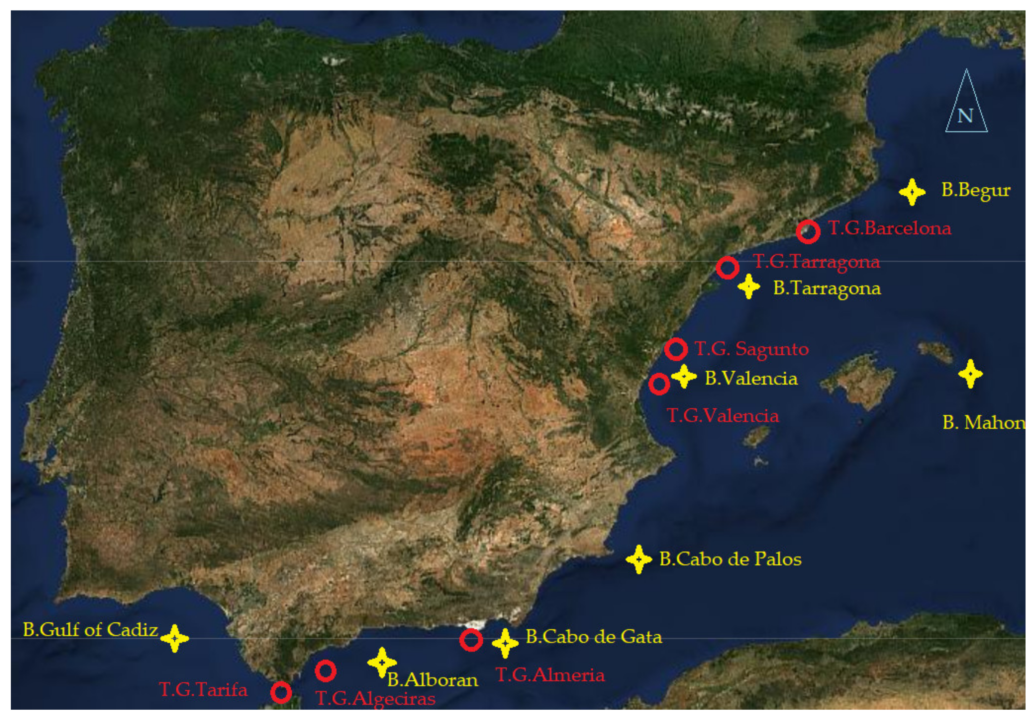
Figure 2 shows all the buoys and tide gauges chosen for the study, and the buoys and tide gauges used are also listed in Table 1 and Table 2, respectively.
The study was conducted in three different blocks: first, the values of Hs and Tp were studied; then the SL variable; and finally, the correlation between the extremes of all the variables (Hs, Tp and SL).
To analyse and construct the data of Hs and Tp, the first step was to choose the corresponding buoy of the section of oceanography of the Spanish ports’ website. Once the buoy was selected, the report was downloaded and the option “monthly maximums” was selected to download the data [30]. All the data were plotted and studied statistically. In addition, the parameters of α, β, γ and λ; Hs and Tp for 20, 50 and 100 years and their evolution in time were studied in each buoy.
It is important to examine the evolution of α, β, γ and λ because they are the statistical parameters that characterize the extreme long-term distribution. α is the Hs threshold, β is the scale parameter and γ is the shape coefficient. α, β and γ are the three parameters that characterize Weibull distribution (Equation (1))
λ is the number of the average number of storms occurring in a year and it is normally used in the POT (Peaks Over the Threshold) distribution (Equation (2)).
Tp for 20, 50 and 100 years are the Tp expected in 20, 50 and 100 years, respectively. These values are obtained applying the POT distribution (Equation (2)) for the 20, 50 and 100 years return period. Once the Hs is obtained, Equation (3) is applied
The parameters a, b, α, β, γ and λ are obtained for each buoy from “Puertos del Estado” reports [31].
To analyse and construct the data of SL, the procedure followed was very similar to the method explained above but instead of taking the buoy records, tide gauge records were downloaded [32].
Finally, a statistical study was carried out to analyse the correlation of the hydroclimatic extremes. In this part of the study, the methodology was different. First, the monthly extremes of SL and the day and hour when the event happened were collected. Then, a search for the wave occurring at that hour was carried out and the values were plotted. Therefore, the main variable in the correlation analysis conducted was the SL, and the secondary value was the wave height.
3. Results
This section is divided into four subsections. Section 3.1 is the study of Hs and Tp, in which the evolution of the parameters Hs and Tp of each buoy is presented. Section 3.2 is the study of extreme statistical parameters. Section 3.3 is the study of SL, similar to Section 3.1, but analysing the SL variable. Section 3.4 is the correlation of hydroclimatic extremes, in which the correlation of the extremes of Hs, Tp and SL is studied.
3.1. Study of Hs and Tp Monthly Extremes
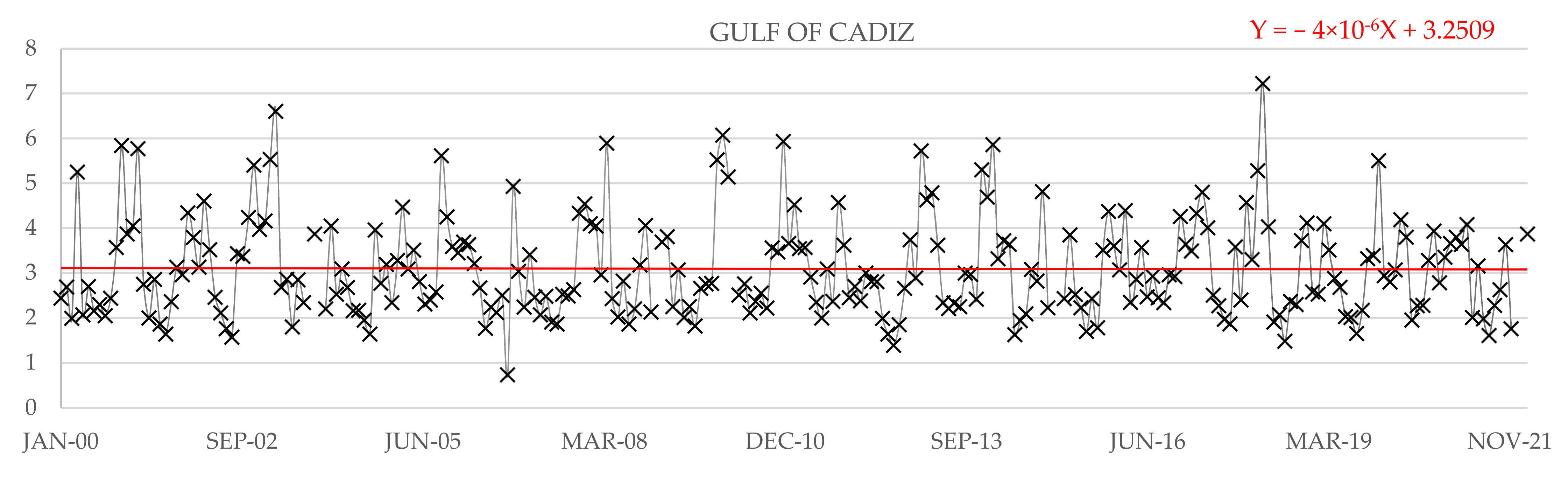
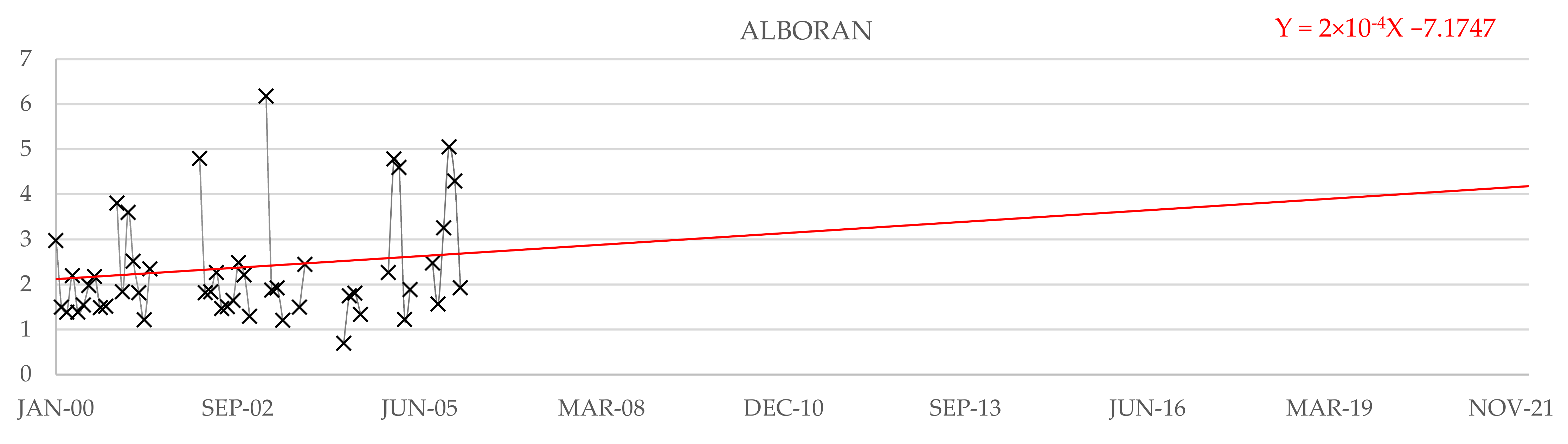
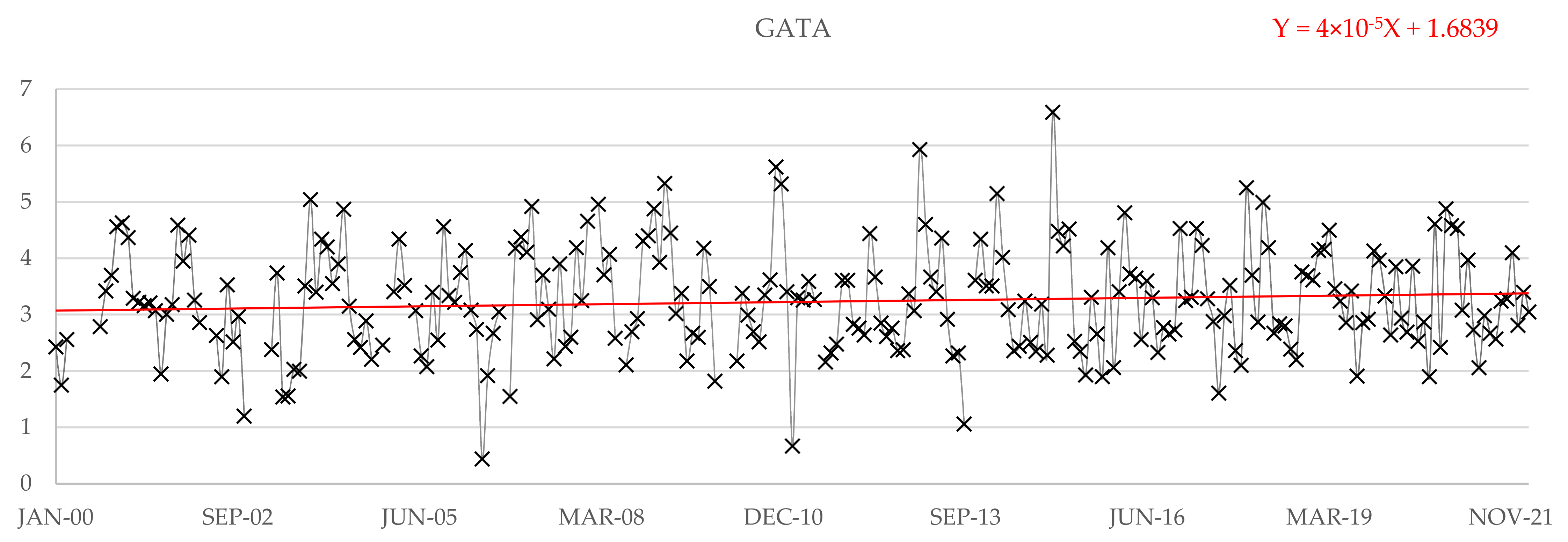
The evolution of monthly Hs extreme records is presented in Figure 3, Figure 4, Figure 5, Figure 6, Figure 7, Figure 8, Figure 9 and Figure 10. The Y-axis is the Hs in m and X-axis the time. All the X-axes of this section have been unified to facilitate the comparison of the different spots. All the figures presented have an X-axis that goes from January 2000 to March 2022 even if there were more records or less than this year frame. As mentioned above, it was decided to unify all graphs in order to facilitate the interpretation and comparison of the results.
Each graph also shows the trend line following the maxima of Hs and its analytical expression (in the colour red). This was carried out by means of a linear adjustment because it was considered to give the most visual and tangible image of the trend followed by the extremes. This will facilitate the analysis of the results and the reaching of the conclusions presented in Section 4 and Section 5.
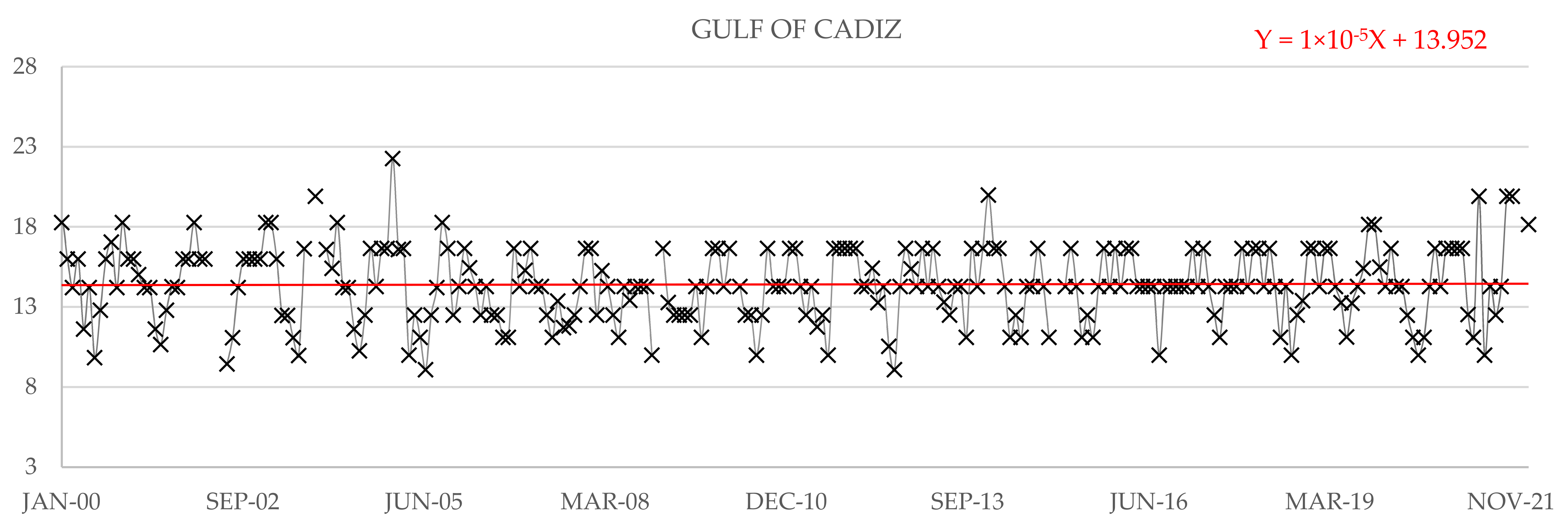
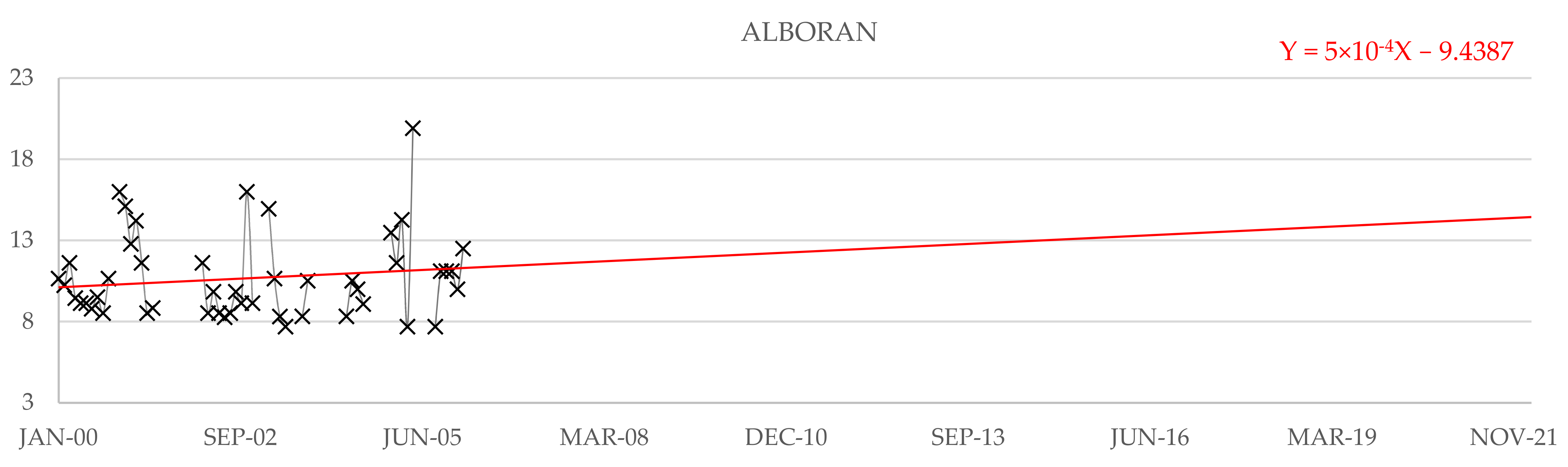
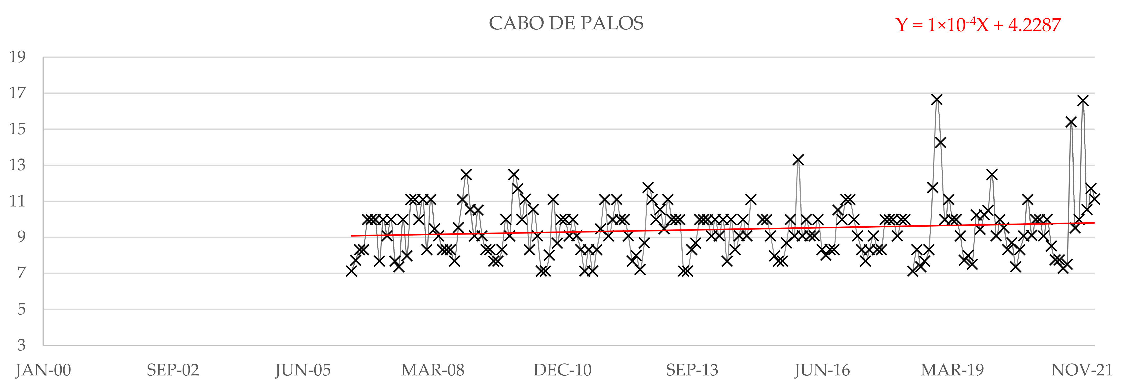
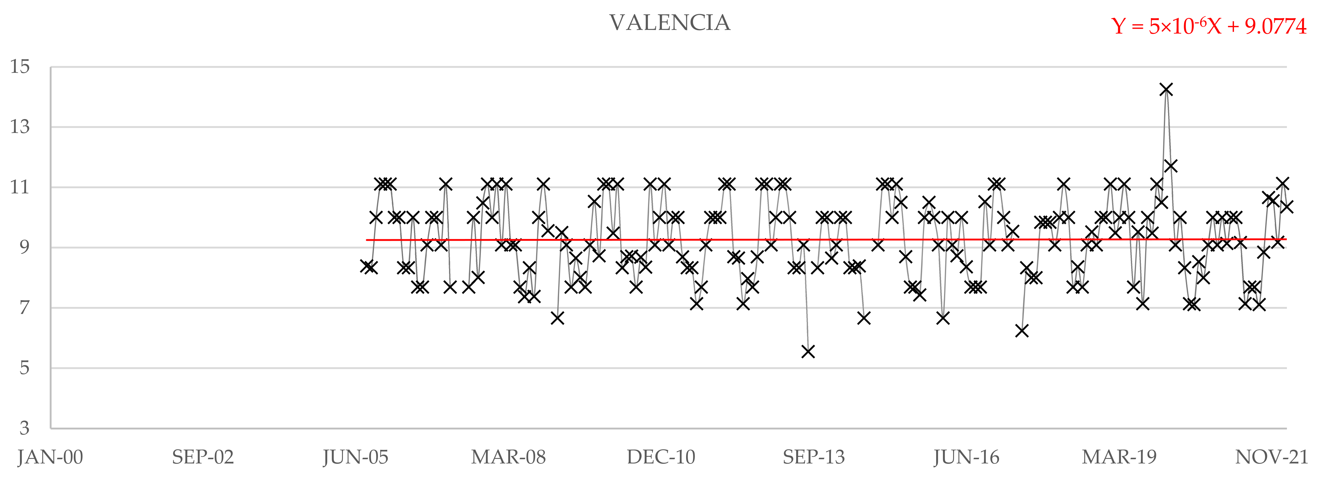
The evolution of monthly Tp extremes is presented in Figure 11, Figure 12, Figure 13, Figure 14, Figure 15, Figure 16, Figure 17 and Figure 18. As was done with Hs, the trend line is presented in the graphs and the adjustment performed is linear due to the same reason (colour red). The Y-axis is the Tp in s, and the X-axis the time. The X-axis of the graphs has also been unified and all X-axes of Figure 11, Figure 12, Figure 13, Figure 14, Figure 15, Figure 16, Figure 17 and Figure 18 range from January 2000 to March 2022.
3.2. Study of Extreme Statistical Parameters
The study of the parameters of the extreme statistical distribution is presented in this section. Figure 19, Figure 20, Figure 21, Figure 22, Figure 23, Figure 24, Figure 25 and Figure 26 present the number of times Hs has exceeded the exceedance threshold α per year.
The Y-axis is the number of exceedances per month, and the X-axis the time. In this section, all the X-axes have also been unified to facilitate the comparison of the different spots. All the figures presented has an X-axis that ranges from 2000 to 2022, even if there were more records or less than the frame of that year. As mentioned above, it was decided to unify all graphs in order to facilitate the interpretation and comparison of the results.
All the figures also present a linear adjustment to facilitate a subsequent trend study of extremes (colour red).
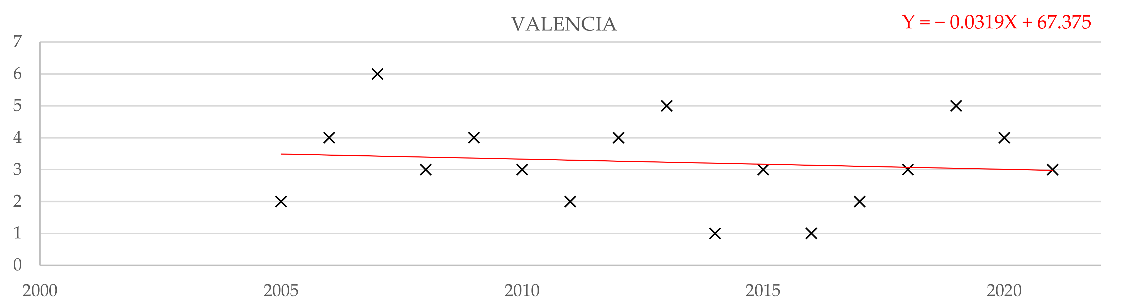
Figure 27, Figure 28, Figure 29, Figure 30, Figure 31 and Figure 32 present the times that Tp has exceeded the expected Tp in 100 years. As with Hs, the Y-axis presents the number of exceedances and the X-axis is time, and all X-axes are unified. In addition, all the graphs present a linear adjustment to facilitate the analysis of the trend of the hydroclimatic extremes (colour red). Valencia results are not presented because in the case of this buoy, the Tp in 100 years was only exceeded twice, once in 2019 and once in 2021.
These graphs will be analysed in Section 4. In addition, the parameters α, β, λ and γ per se and the Spanish ports’ reports of the years 2010, 2011, 2012, 2014, 2015, 2017 and 2020 have been studied [33]. The results were the following:
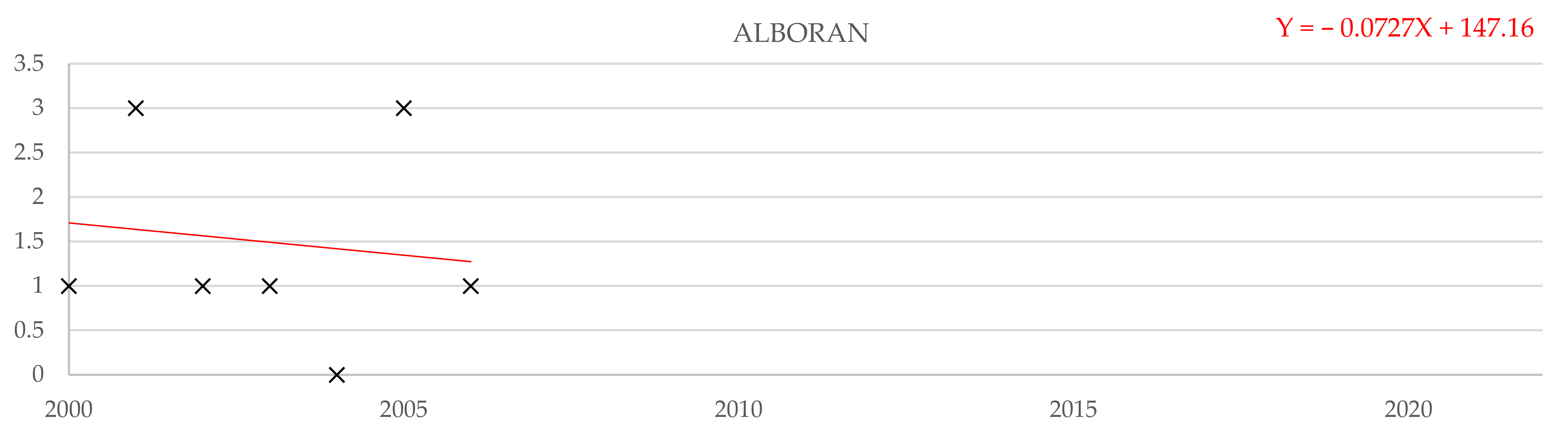
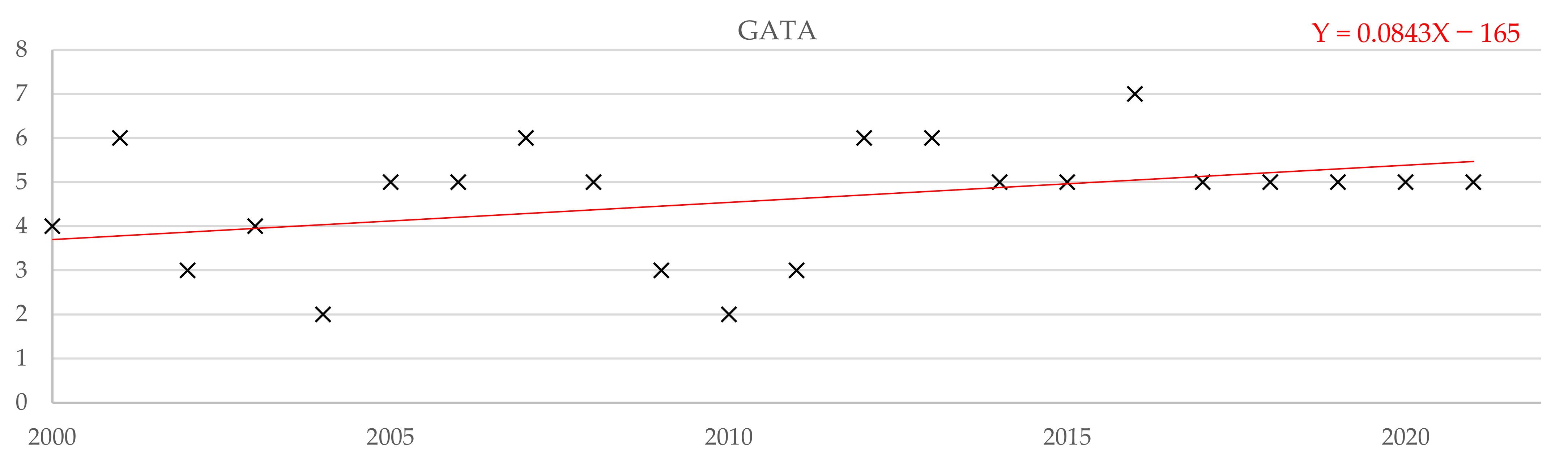
In the Gulf of Cadiz, all the parameters remained stable. In Alboran, λ increased and the parameters β and γ were less than one. In Cabo the Gata, λ was slightly increasing, while γ was slightly decreasing and β remained stable. In Cabo de Palos, β and γ were decreasing and λ was increasing. In Valencia, β and γ were also decreasing and γ was less than one. In Mahon, γ was stable and β decreased. In Tarragona, both γ and β decreased and γ was less than one too. In Begur, γ was stable and β decreased.
It has to be said that the reports of the different years of Gata and Begur had different initial years, which may alter the final results when comparing reports from one year to the next.
3.3. Study of SL Monthly Extremes
In this section, the evolution of the monthly maximums of SL in each tide gauge is presented from Figure 33, Figure 34, Figure 35, Figure 36, Figure 37, Figure 38, Figure 39 and Figure 40. It is structured as the previous sections:
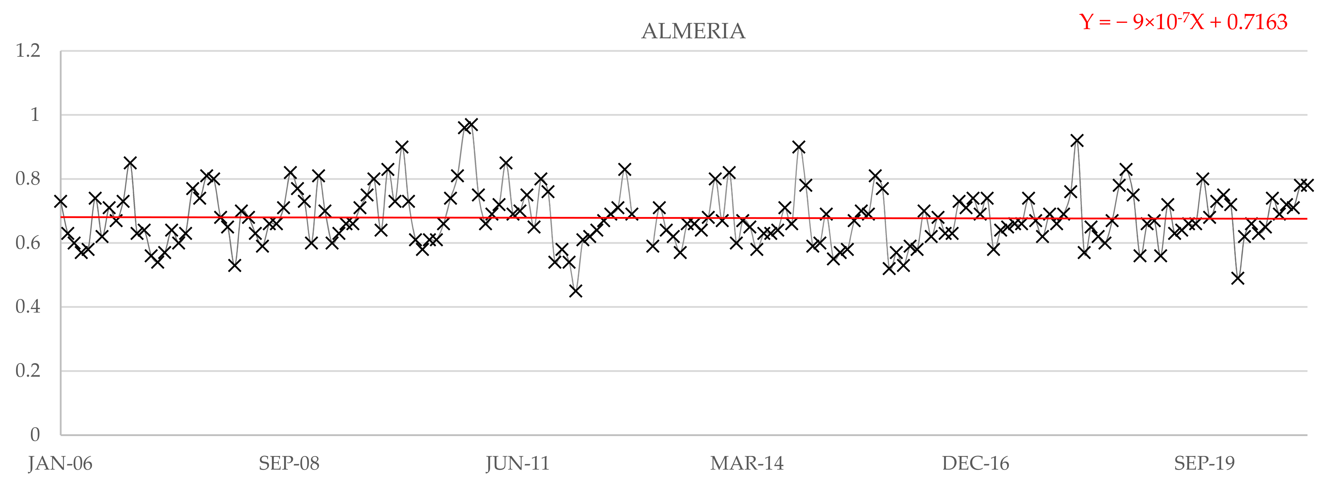
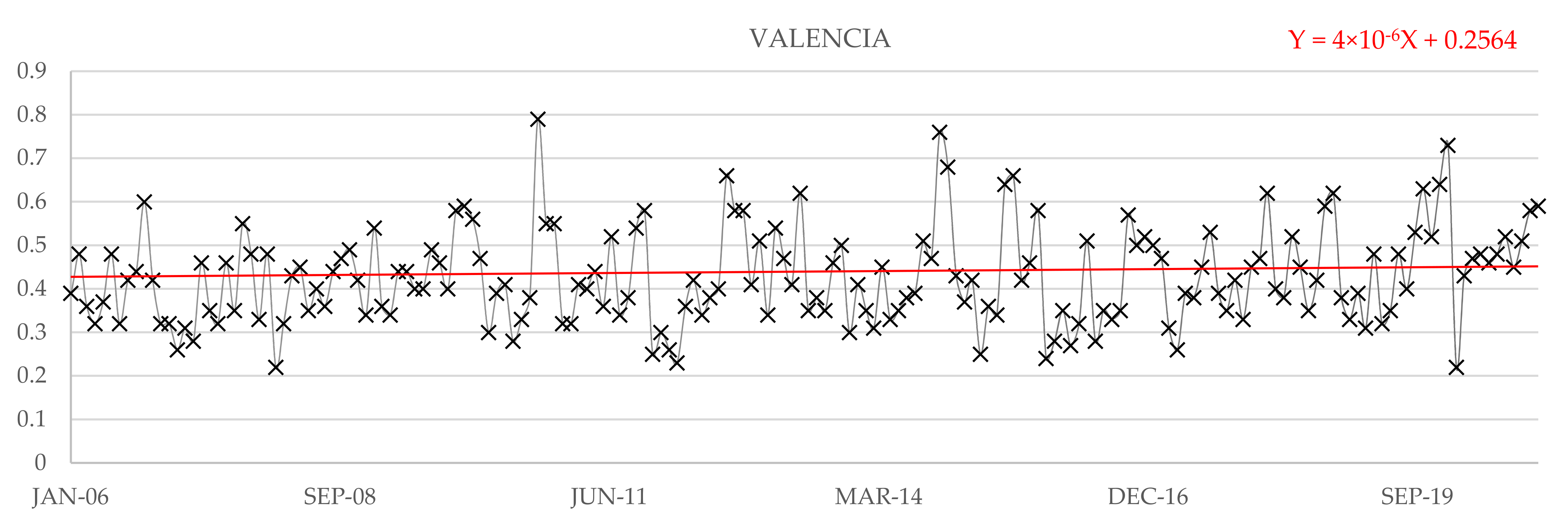
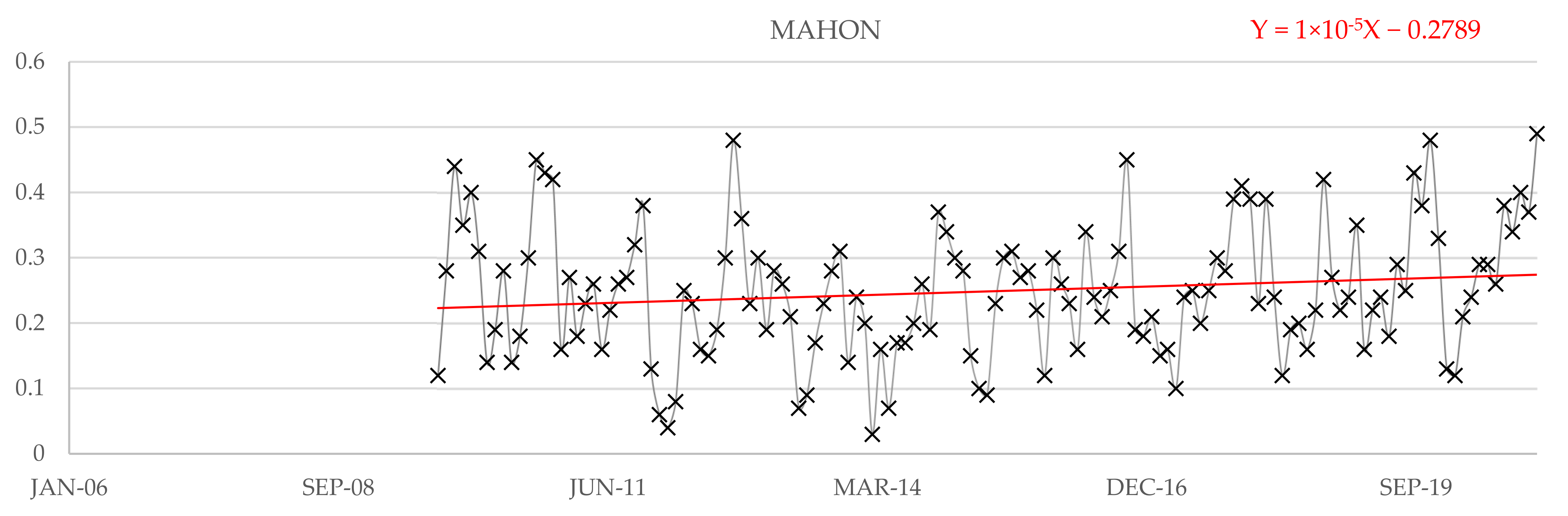
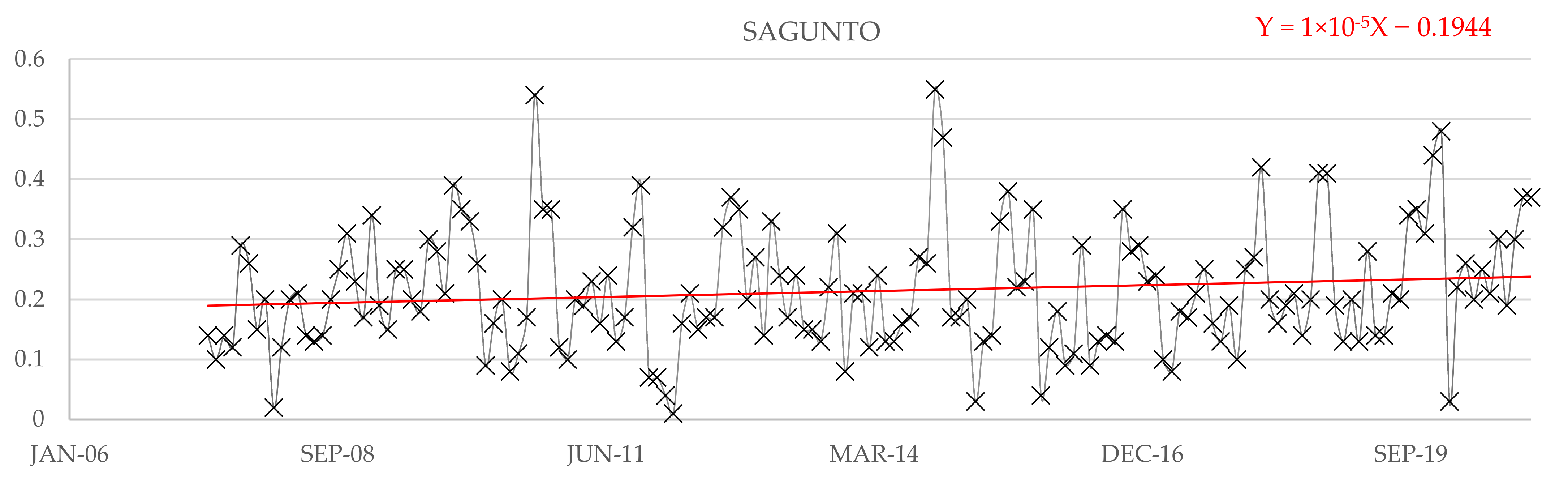
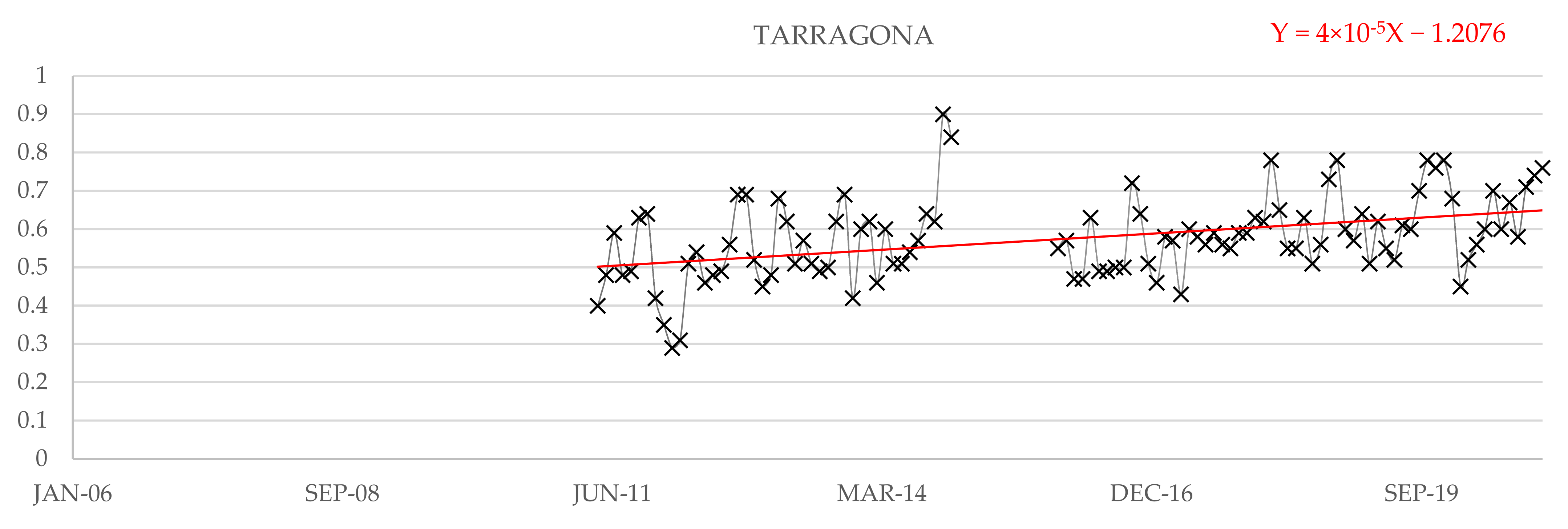
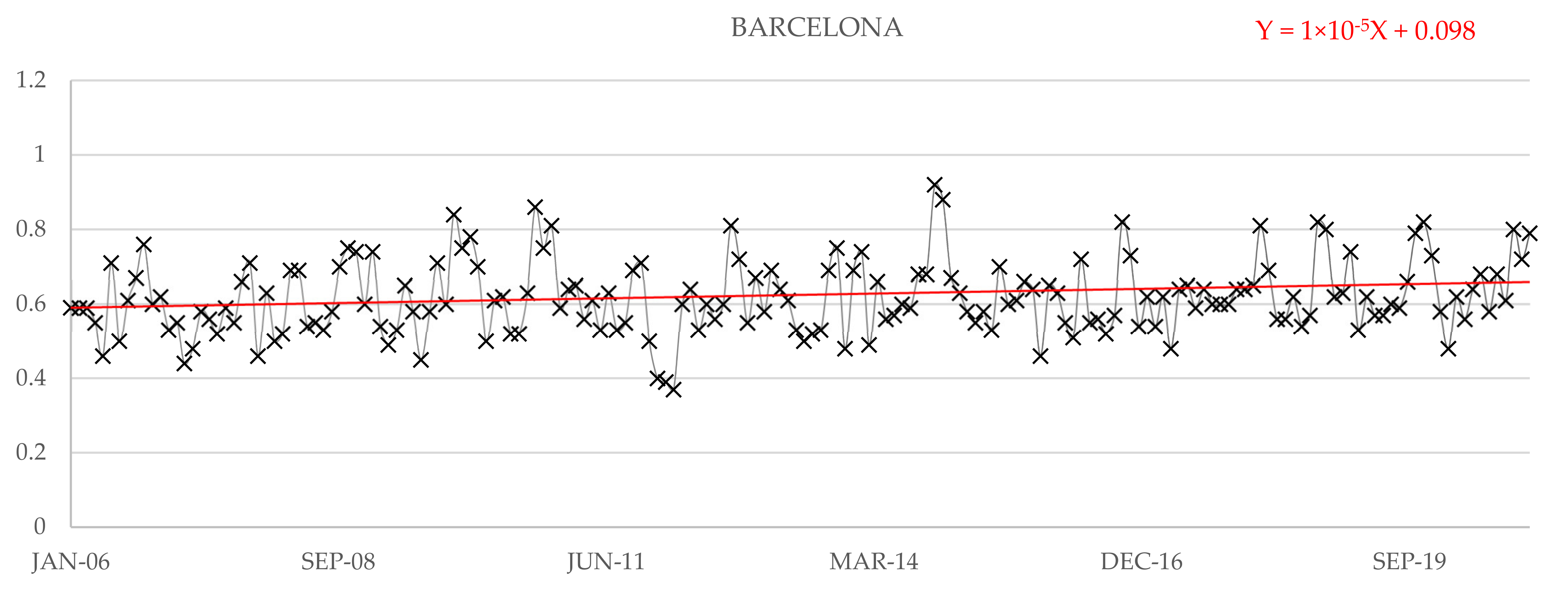
The Y-axis is the SL extremes in m, and the X-axis the time. The X-axes of all the graphs is unified from January 2006 to December 2020. Each graph also shows the trend line (colour red).
3.4. Correlation of Hydroclimatic Extremes
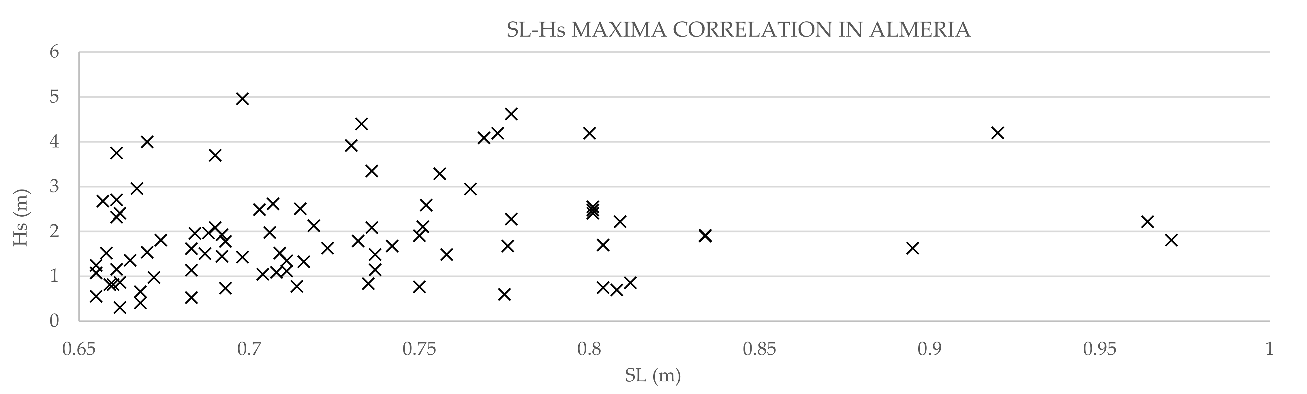
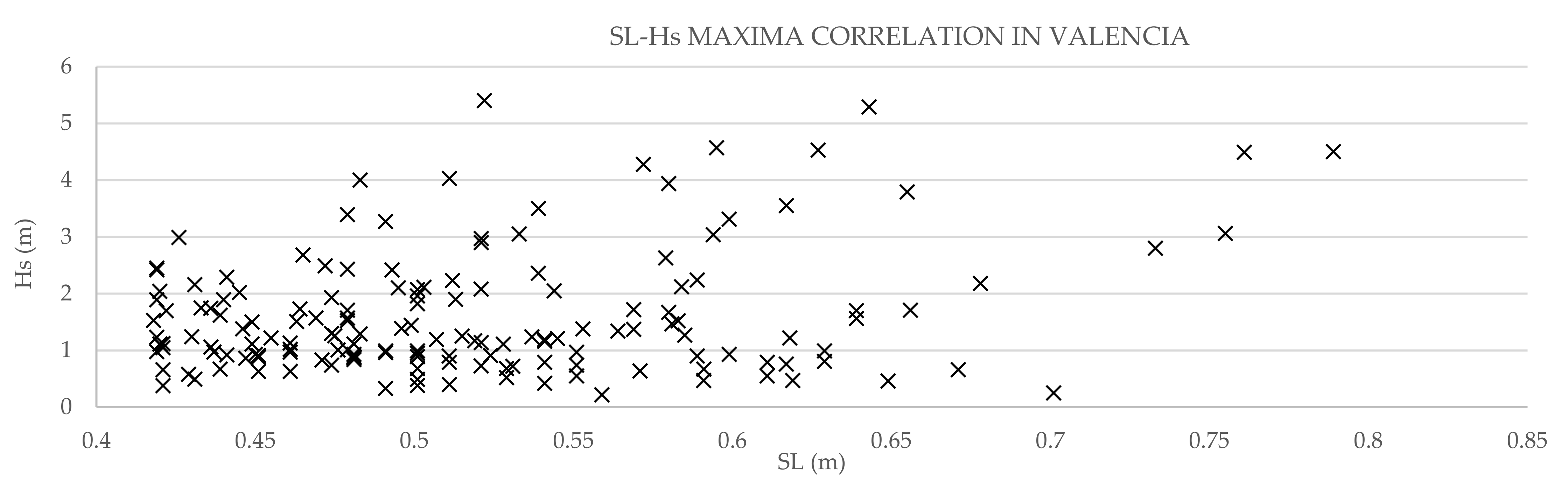
The correlation of SL and Hs maxima has also been studied. Only the correlation in which deep buoys were available has been studied. Therefore, the correlation of maxima in Tarifa and Algeciras have not been analysed, because it was considered that, as the buoys were not in deep water, the results were not reliable. Graphs are presented from Figure 41, Figure 42, Figure 43, Figure 44, Figure 45 and Figure 46.
4. Discussion
4.1. Discussion of Hs and Tp Monthly Extremes
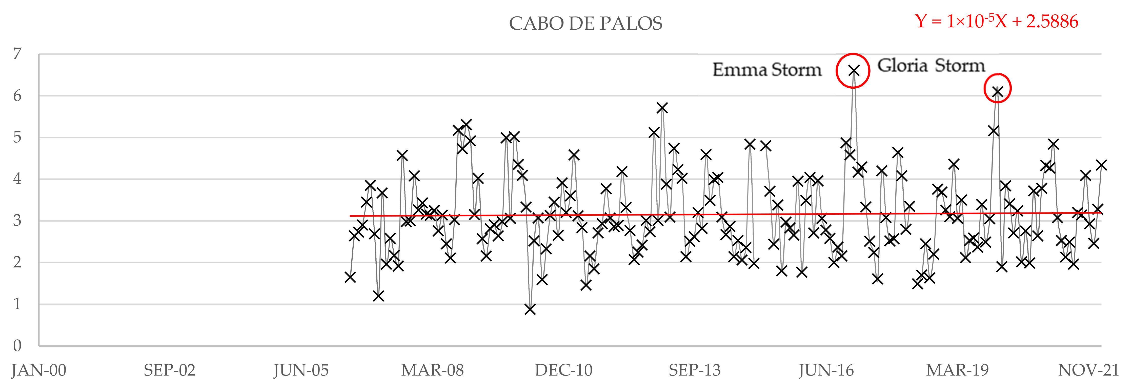
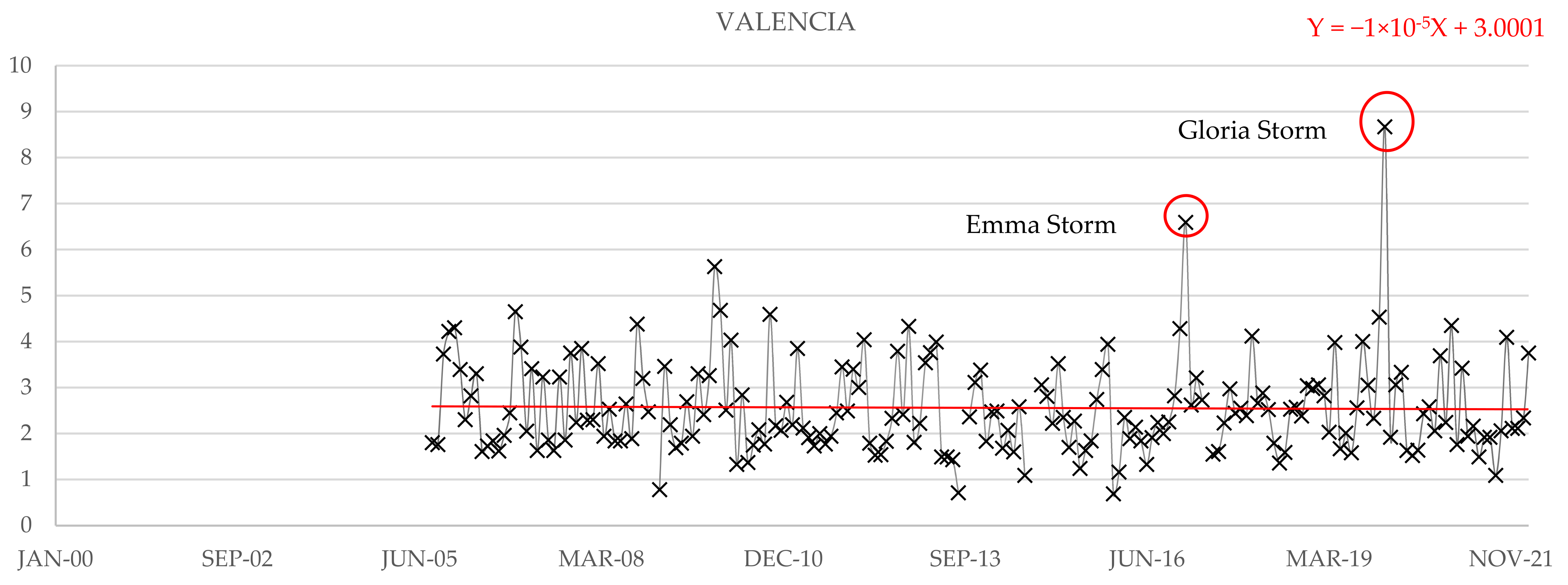
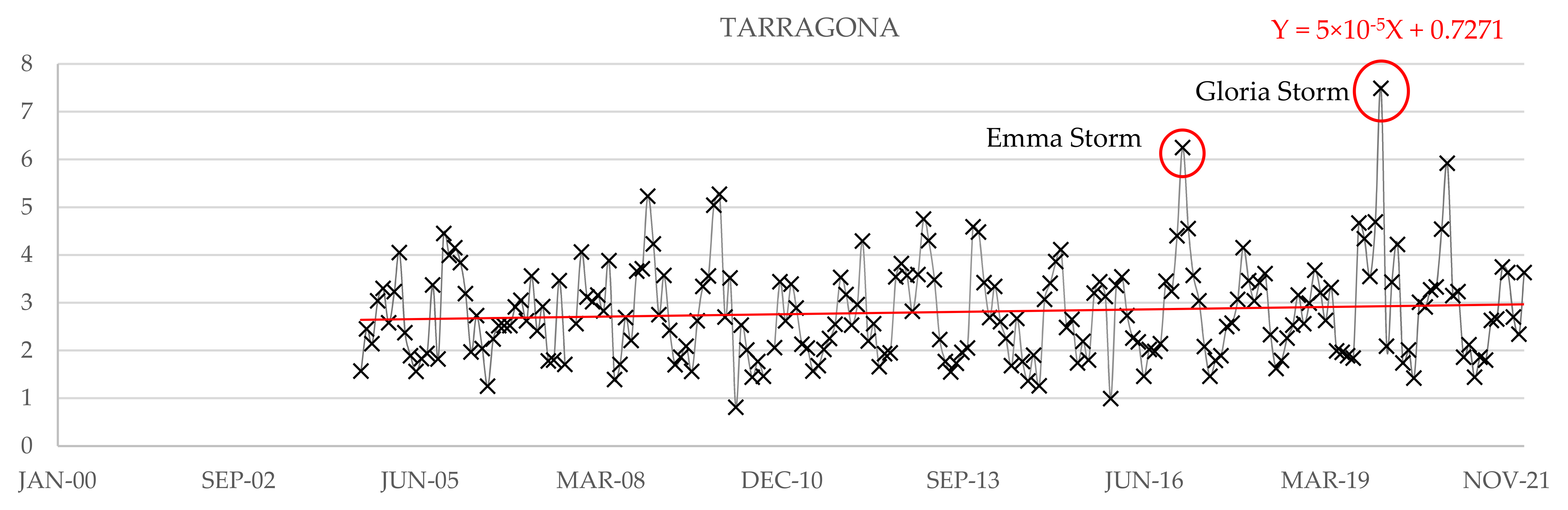
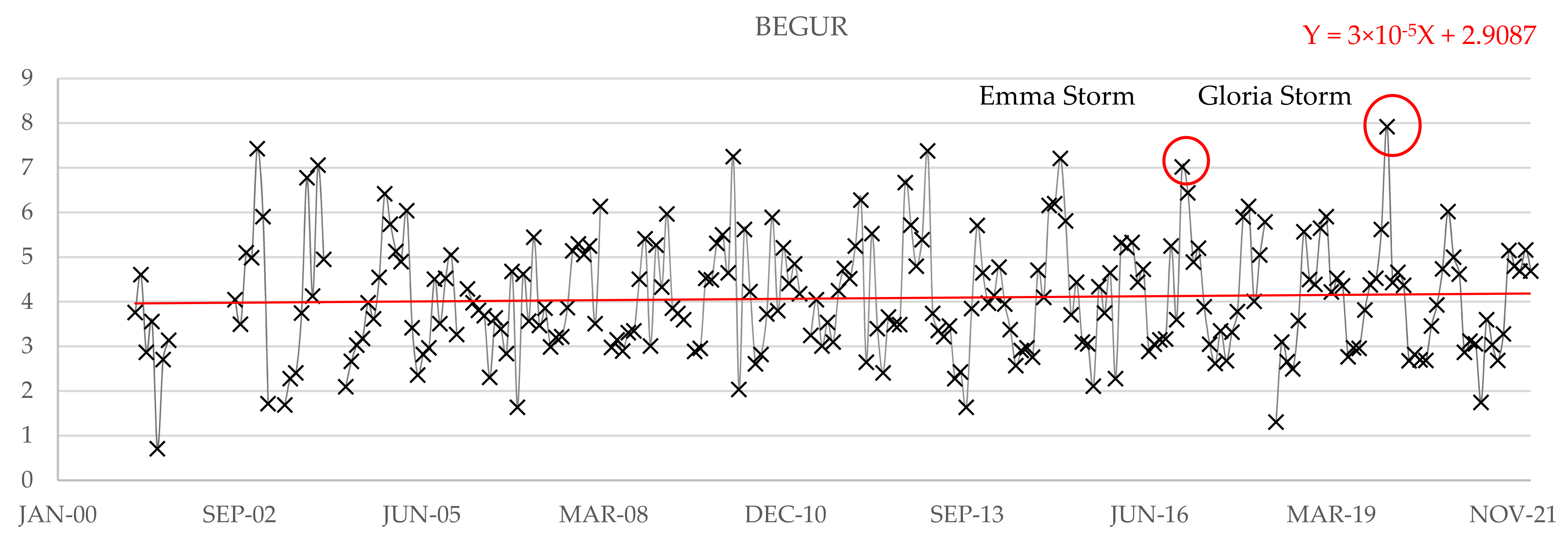
After analysing Hs and Tp plots (Figure 3, Figure 4, Figure 5, Figure 6, Figure 7, Figure 8, Figure 9, Figure 10, Figure 11, Figure 12, Figure 13, Figure 14, Figure 15, Figure 16, Figure 17 and Figure 18), it can be seen that, referring to Hs extremes, all had an increasing trend, except for the area of the Gulf of Cadiz and Valencia, which had a slightly decreasing tendency. When talking about Tp, all the buoys had also a rising tendency and, the increase of Tp extremes was quicker than the increase of Hs, which is related to the results of Section 3.2.
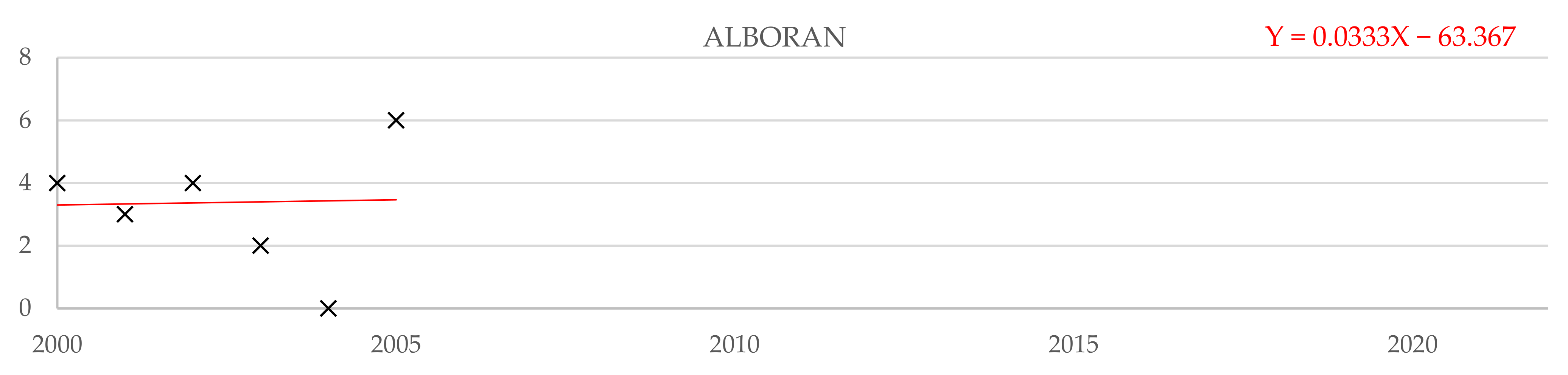
The Alboran graph (Figure 4) is one of the graphs with the steepest trend line in Hs extremes (0.0003 slope). This is probably because the records of the Alboran Sea buoy are from 1997 to 2006. From 2006 onwards there are no more records. If there were records from 2006 to 2022, the increasing trend line would probably be much smoother. Furthermore, the Alboran Sea is an area affected by local and regional phenomena due to its position. It is an enclosed sea where the wave and wind patterns are very particular, so part of this increasing trend may also be due to these local phenomena and not just to the data series.
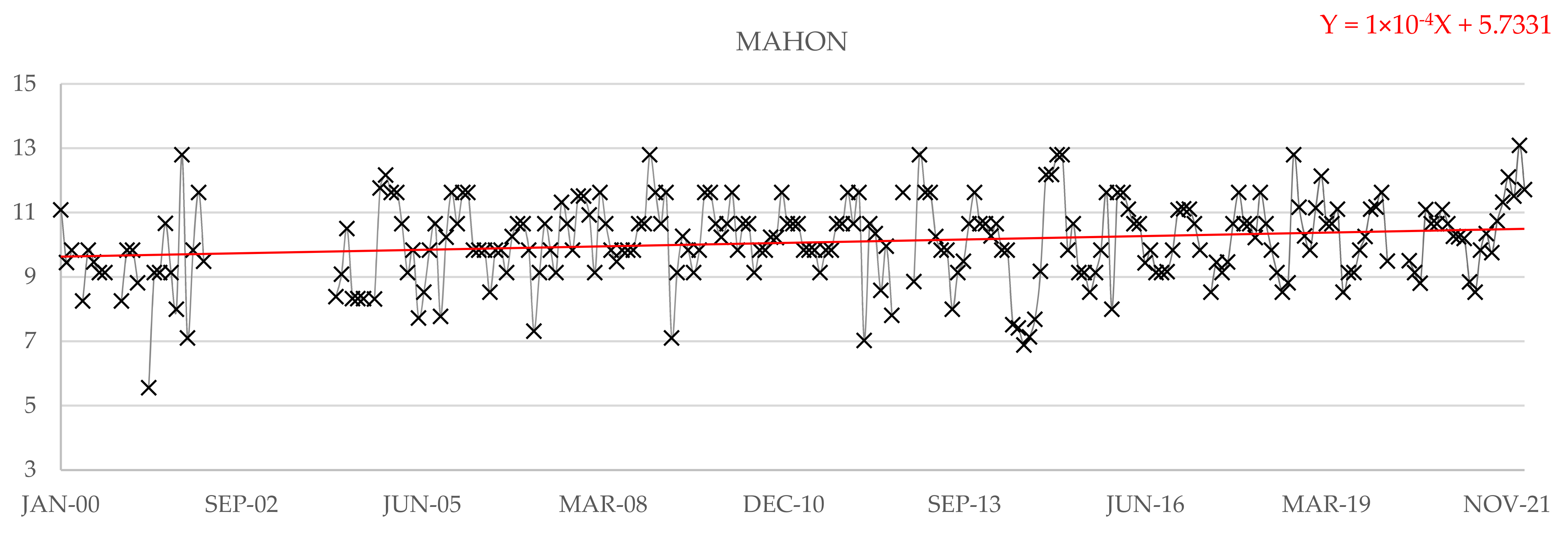
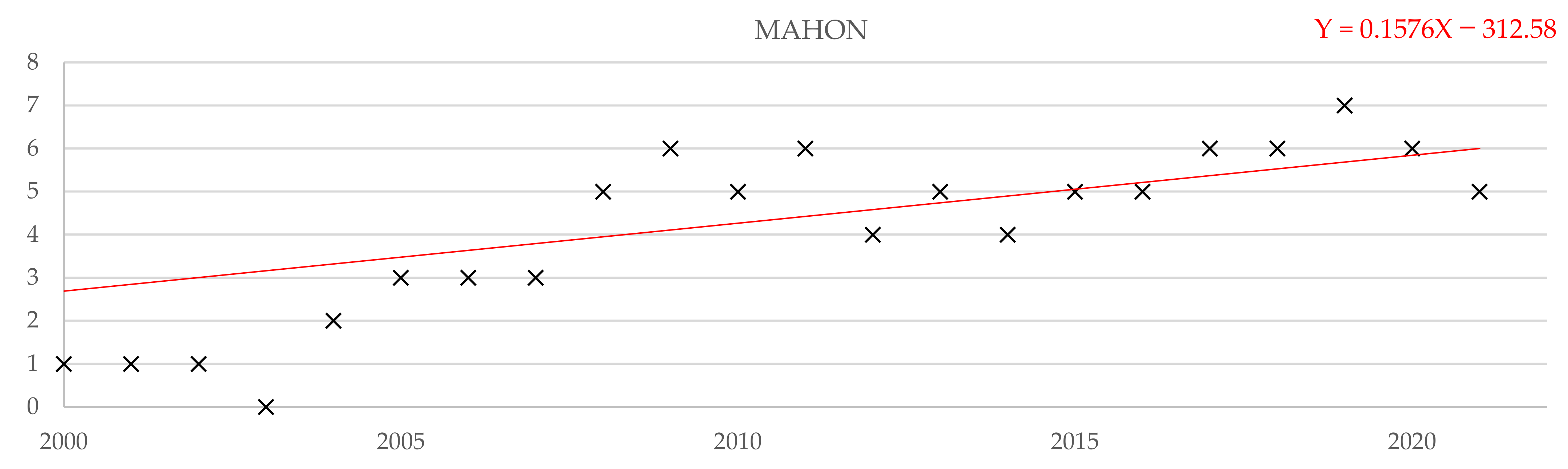
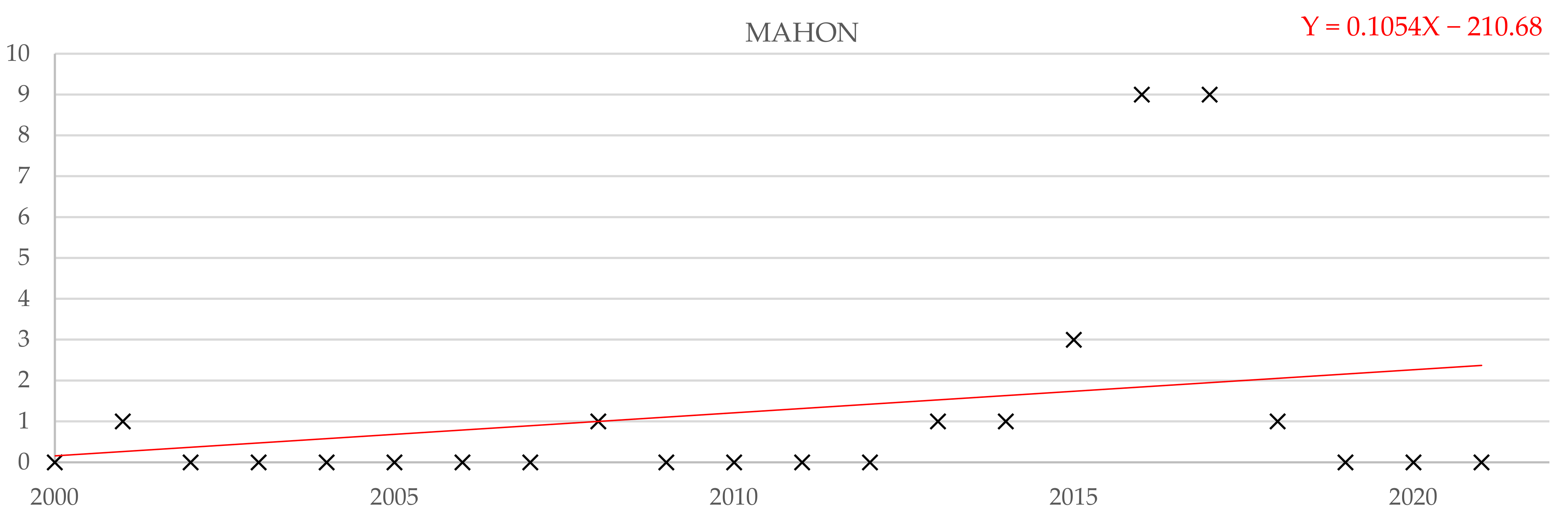
Mahon is the other spot where the increasing trend is sharper (0.0001 slope). In this buoy, the problem of the records does not exist. Therefore, this increasing trend can be taken with a high level of certainty, as the records reach from 1993 to 2022. The fact that Hs is increasing more sharply here than in the rest of the Spanish Mediterranean coast is likely due to the wave and wind patterns of this particular area. This clear increasing trend in Hs highlights the need for further studies of climate extremes in this area.
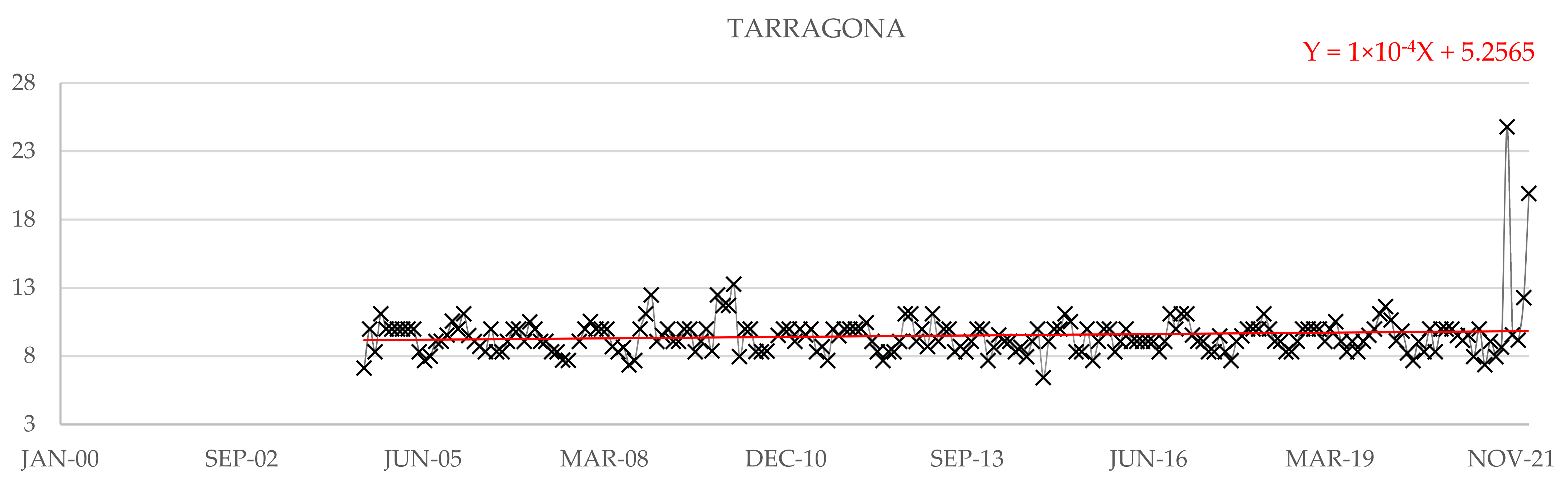
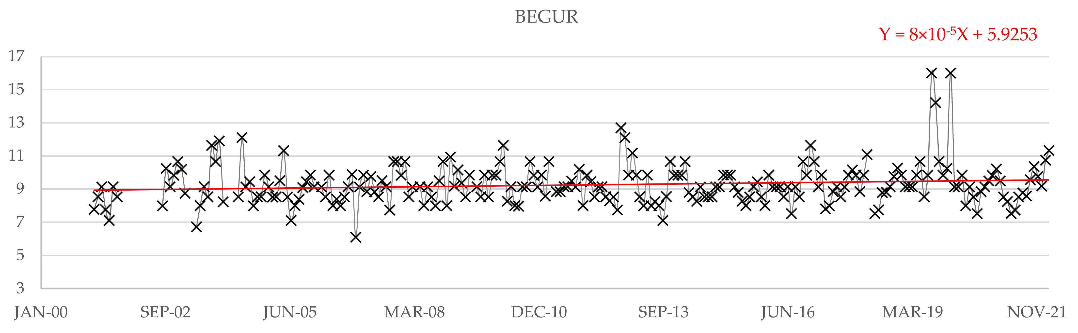
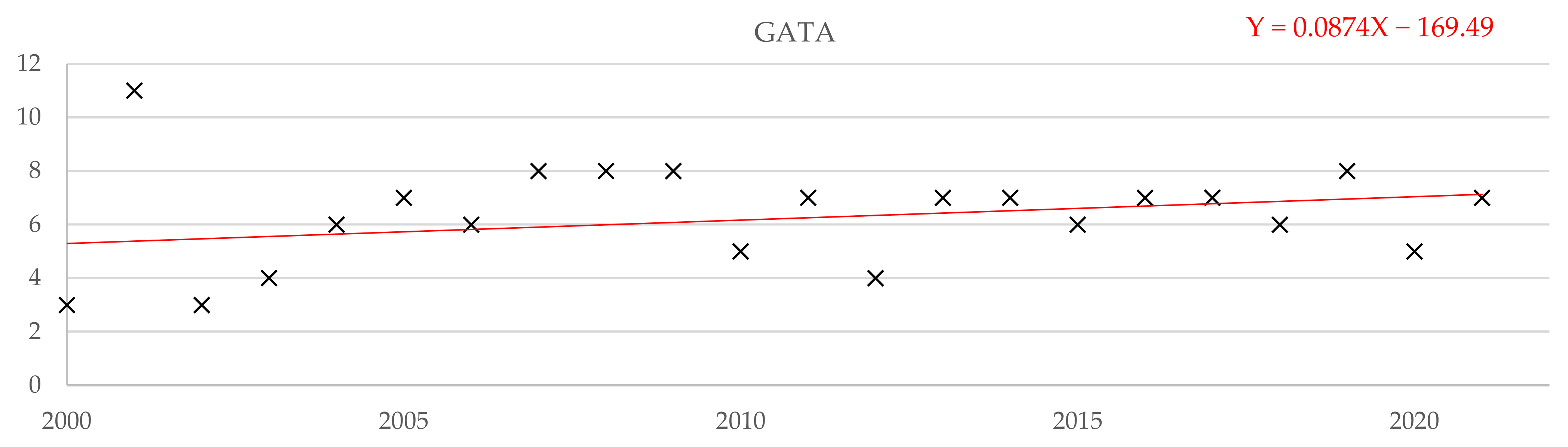
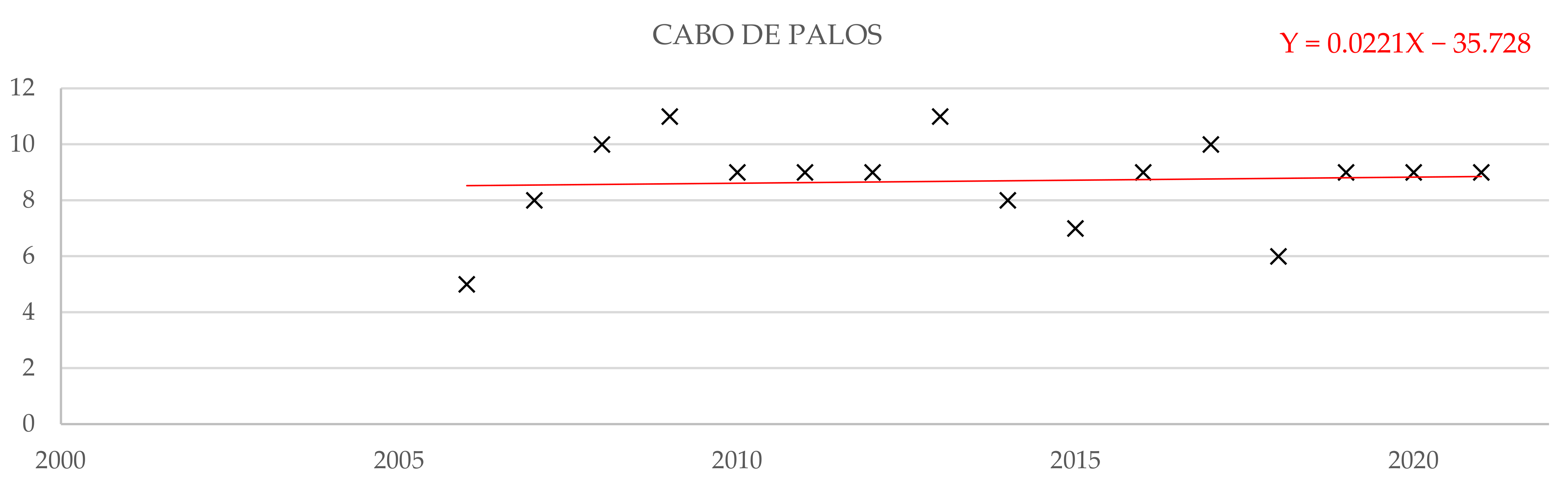
From Cabo de Gata to Begur (Figure 5, Figure 6, Figure 7, Figure 9, Figure 10), the increasing trend of Hs is similar (around 10−4–10−5), excepting the Valencia buoy, which has a slightly decreasing trend. This area may be affected by the same meteorological regional patterns and fluid dynamics. The increasing trend is not as pronounced as in Alboran or Mahon. However, it has to be said that although the trend is less upward, this does not mean that this area is less threatened by extreme events. Although the general trend is less abrupt, this area is prone to very specific but very intense events, as can be seen in the graphs for the 2018 and 2020 storm (Emma and Gloria storm), which far exceeds the rest of the extreme storms. In fact, these “very extreme” events are the most damaging and threatening, and this part of the coast is especially vulnerable to extreme storms. This is also the main reason why the data of these graphs seem to be very scattered, because in this area hydroclimatic extremes are very occasional and intense.
Referring to the Tp climate variables, the conclusions are the same as with Hs. The only difference, as noted above, is that the increasing trend of Tp is more pronounced than that of Hs. This makes sense since Hs and Tp are related, according to the expression Tp = a*Hsb.
4.2. Discussion of Extreme Statistical Parameters
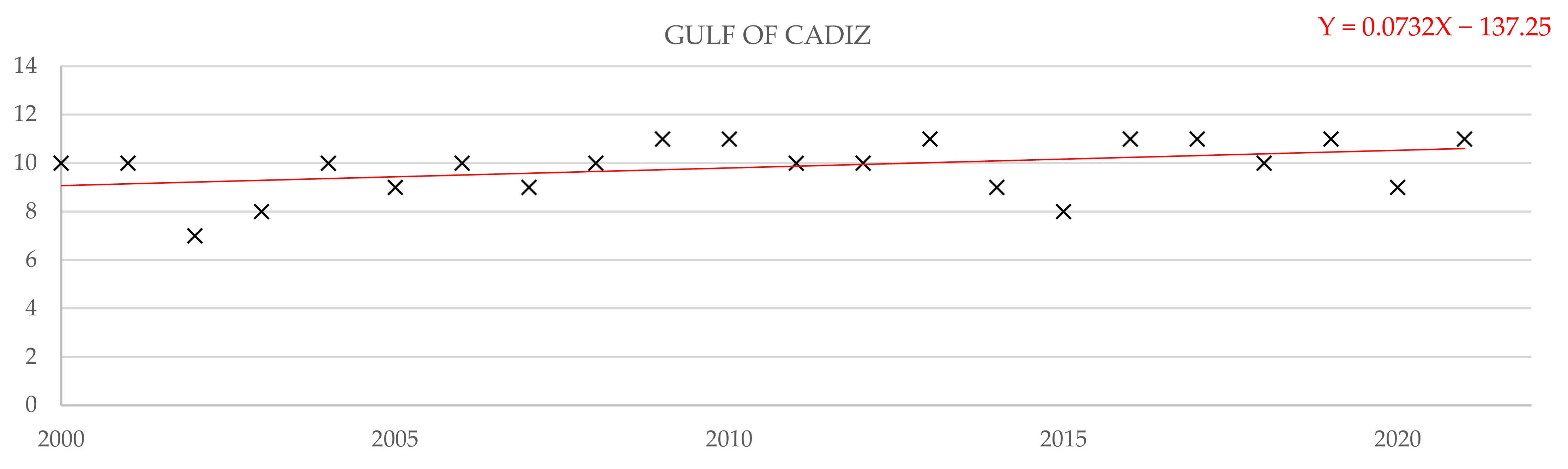
The wave height threshold was typically exceeded in 30% of cases. The wave heights for 20, 50 and 100 years were exceeded at most once in the entire data series, while with the peak periods, up to 85% of the current data exceeded the expected peak period in 100 years (Gulf of Cadiz). Typically, around 20% of the peak periods of the year exceeded the expected 100-year peak period, which is a representative percentage considering that Tp is the Tp expected in 100 years. The fact that a 20% of the current maxima overpasses the Tp expected in 100 years is proof that the estimated Tp for 100 years already exists in current temperature due to the effect of climate change on extreme hydroclimatic phenomena.
The Hs for 20, 50 and 100 years was rarely exceeded in all the spots studies, but the Tp estimated for 20, 50 and 100 years from now was exceeded in some cases by up to 85% of the monthly maxima. This also shows that a statistical readjustment of this variable Tp is already necessary, as the current values do not accurately represent the extreme Tp. Although the increase in Hs may not be significant, the increase in Tp is significant and an adjustment of the statistical values and parameters is needed to adjust the models to the new reality. If this is not carried out, climate modelling and future projections will become increasingly inaccurate.
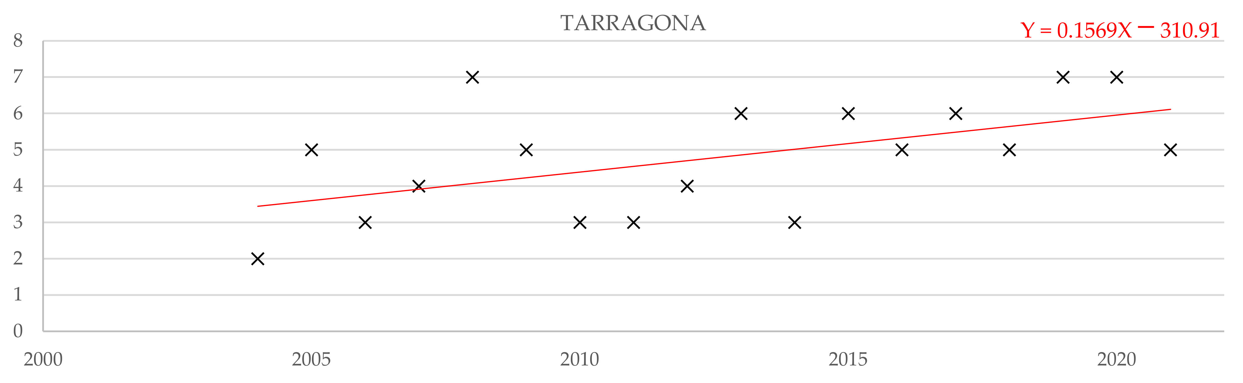
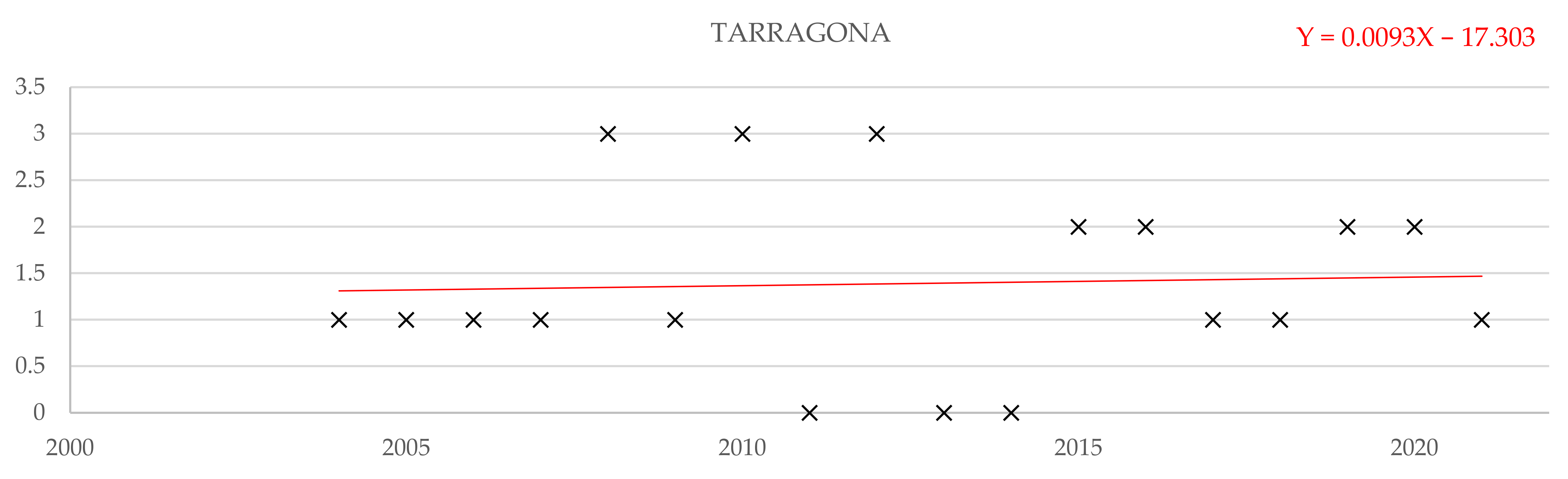
Referring to the specific spots studied. The Gulf of Cadiz is one of the buoys that need a more urgent adjustment of the Tp statistical distribution, as the estimated Tp 100 years from now was already exceeded in the 85% of the extreme storms. Valencia, on the contrary, has very well adjusted Tp parameters and the Tp in 20, 50 and 1000 years was hardly exceeded. Tarragona and Mahon are other spots that could be said to be well-adjusted, as the 100-year Tp was only exceeded in 10% of the extreme storms. Finally, the area of Valencia would also need a revision of the statistical parameters but the number of exceedances is not as high as in Cadiz.
4.3. Discussion of SL Monthly Extremes
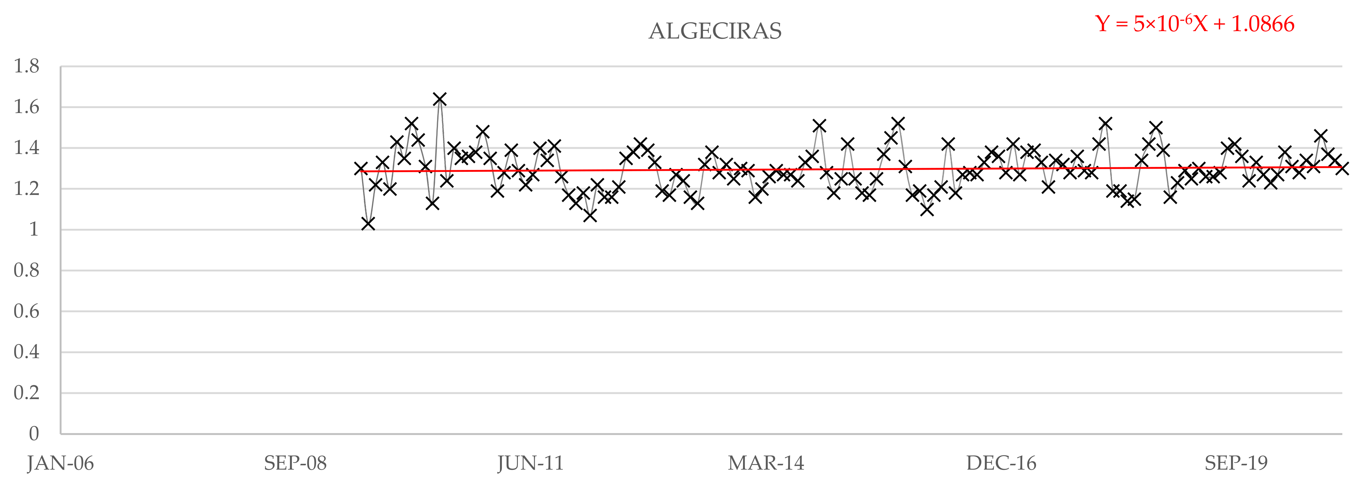
Referring to SL results, almost all the tide gauges showed an increase in sea level. However, it is striking that the tide gauge at Tarifa shows an appreciable drop in sea level, which may be due to regional effects in the area and would need to be studied in more depth in order to reach reliable conclusions.
As is logical, the area where the maximum sea levels vary the most is the area from Cadiz to Almeria due to the astronomical tides. On the other hand, there is the area of Valencia and Cabo de Palos, whose tidal range is 0. Here, even though the tide is practically nil, it can be seen that sea level peaks are also reached very occasionally, following a similar behaviour to that explained by Hs and Tp extremes in Section 4.1., which increase the vulnerability of these areas to hydroclimatic extreme events. If concomitant extreme events (Hs, Tp and SL) occur in this area, the damage and losses can be devastating, as extreme events in this area of the Mediterranean are very intense. This will be further discussed in the next subsection.
Finally, referring to the area of Barcelona and Tarragona, SL maxima variability is also higher because of the tides.
The general pattern is that SL maxima are increasing, as has been proven by the scientific community. The area where this increasing trend is sharper is the Levantine basin, which makes it more vulnerable to extreme storms, as this paper has already stated.
4.4. Discussion of the Correlation of the Hydroclimatic Extremes
Finally, the correlation of Hs and SL was analysed. As mentioned in the previous subsection, assessing the concomitance and correlation of hydroclimatic extremes is essential to avoid future damage. In addition, the Levant Mediterranean area is particularly vulnerable to occasional, but very intense, extreme events.
In Almeria, extreme SL were associated mostly with medium waves, while extreme waves happened with medium SL.
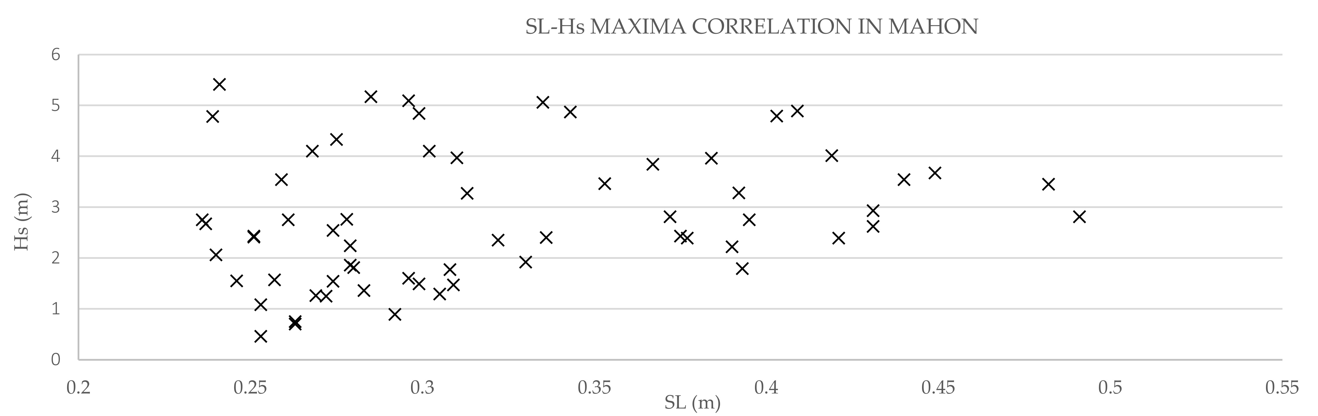
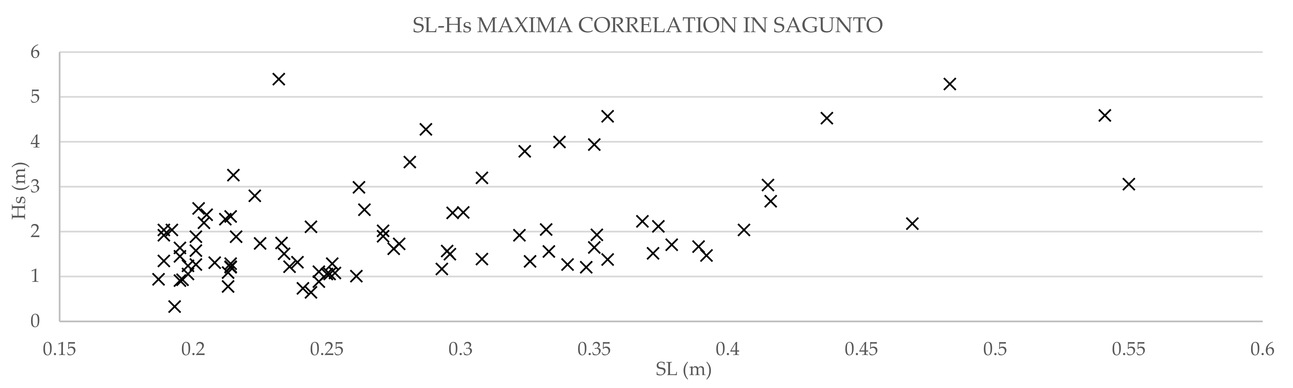
In Valencia, Mahon and Sagunto, extreme SL occurred with relatively high waves, which should be considered in future designs so as not to underestimate extremes and their concomitance. The fact that extreme events in this area can be concomitant further aggravates their situation, as they already have a devastating effect on their own. If maximums of all three variables were to occur at the same time, the damage could be even greater, which requires specific studies in the Levante area.
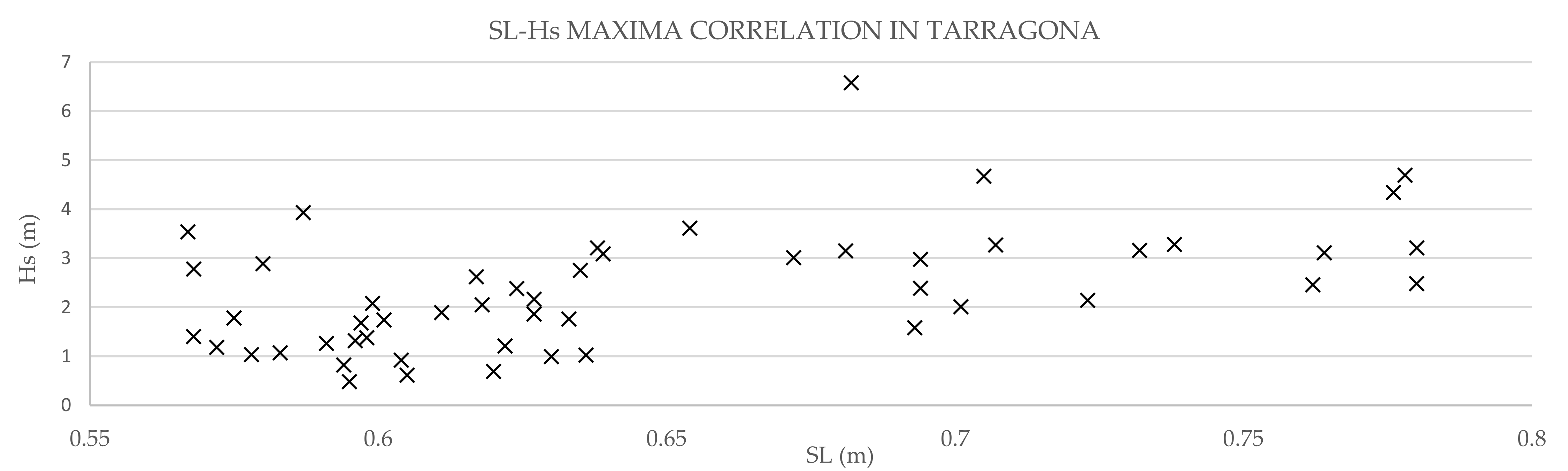
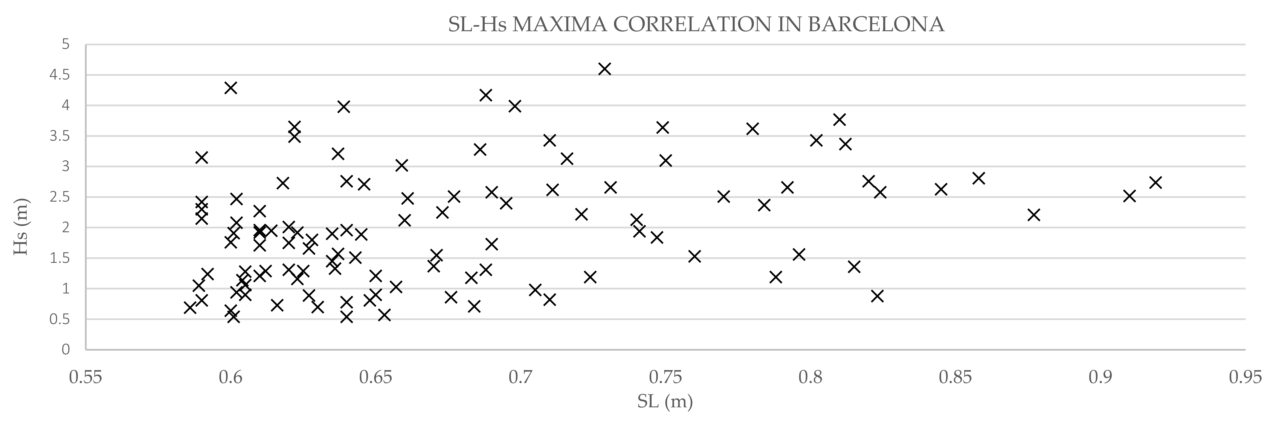
In Barcelona and Tarragona, the concomitance of the hydroclimatic extremes were not as clear as in the Levantine basin with Valencia, Mahon and Sagunto, but it can be appreciated how some of the highest waves and SL also occurred with relatively high SL or waves, respectively. However, it is not as relevant as it is in the Levantine basin.
5. Conclusions
After analysing and discussing all the results, several conclusions can be highlighted.
Mahon and Alboran are the spots in the Spanish Mediterranean were the increasing trend of Hs and Tp extremes is sharper. This increasing trend can be taken with a high level of certainty in Mahon and with a medium level of certainty in Alboran due to the short-period data frame.
Although the increasing trend of Hs maxima in the Levantine basin is not as sharp as in other parts of the Spanish Mediterranean coast, it is subjected to the most intense one-off events. These events are the ones that cause the most damage, making the Spanish Levante region particularly vulnerable to extreme hydroclimatic events.
A readjustment of the Tp statistical parameter is needed. Expected Tp for 100 years is reached in more than 20% of extreme storms in most of the spots studied, which means that the estimated Tp for within 100 years is already happening. The most critical spot is the Gulf of Cadiz with an 85% of exceedance.
SL is increasing along all the Spanish Mediterranean coast, excepting Tarifa, which may be due to local phenomena. The behaviour is very similar to Hs and Tp extreme events but affected by the astronomical tide.
The area with the highest concomitance of extreme events is the Levantine basin. Having SL, Hs and Tp extreme events at the same time would be devastating. Therefore, more in-depth studies on the coast from Valencia to Cabo de Palos are needed, and even more so considering that this is the area of the Spanish coast where the fewest scientific studies have been carried out.
Considering all these conclusions, future research directions should focus on studying the concomitance of hydroclimatic extreme events (Hs, Tp and SL) in the Levantine basin and in the adjustment of statistical Tp parameters.
Author Contributions
This paper will be included in the PhD thesis developed by Nerea Portillo at the Technical University of Madrid, Spain, and the aim of the research relates to reviewing climate change and its impact on ports and its adaptation, carried out by the PhD candidate. All the authors contributed toward choosing data, discussion, methodology, figures and references to provide an accurate paper. Conceptualization, N.P.J. and V.N.V.; Funding acquisition, N.P.J.; Investigation, N.P.J., V.N.V. and J.M.d.C.; Methodology, N.P.J. and V.N.V.; Writing—original draft, N.P.J.; Writing—review and editing, N.P.J., V.N.V. and J.M.d.C. All authors have read and agreed to the published version of the manuscript.
Funding
Author Nerea Portillo Juan has received research support from Universidad Politécnica de Madrid. She is a beneficiary of one of the scholarships of the UPM pre-doctoral programme.
Data Availability Statement
Not applicable.
Conflicts of Interest
The authors declare no conflict of interest.
References
- Portillo Juan, N.; Negro Valdecantos, V.; del Campo, J.M. Review of the Impacts of Climate Change on Ports and Harbours and Their Adaptation in Spain. Sustainability 2022, 14, 7507. [Google Scholar] [CrossRef]
- Villeta, M.; Valencia, J.L.; Saa, A.; Tarquis, A.M. Evaluation of extreme temperature events in northern Spain based on process control charts. Theor. Appl. Climatol. 2018, 131, 1323–1335. [Google Scholar] [CrossRef]
- Quereda, J.; Monton, E.; Vázquez, V. La elevación de las temperaturas en el norte de la Comunidad Valenciana: Valor y naturaleza (1950–2016). Investig. Geográficas 2018, 69, 41–53. [Google Scholar] [CrossRef] [Green Version]
- Lorenzo, N.; Díaz-Poso, A.; Royé, D. Heatwave intensity on the Iberian Peninsula: Future climate projections. Atmos. Res. 2021, 258, 105655. [Google Scholar] [CrossRef]
- Kelebek, M.B.; Batibeniz, F.; Önol, B. Exposure Assessment of Climate Extremes over the Europe–Mediterranean Region. Atmosphere 2021, 12, 633. [Google Scholar] [CrossRef]
- Lionello, P.; Cogo, S.; Galati, M.B.; Sanna, A. The Mediterranean surface wave climate inferred from future scenario simulations. Glob. Planet. Change 2008, 63, 152–162. [Google Scholar] [CrossRef]
- Kundzewicz, Z.W.; Giannakopoulos, C.; Schwarb, M.; Stjernquist, I.; Schlyter, P.; Szwed, M.; Palutikof, J. Impacts of climate extremes on activity sectors–stakeholders’ perspective. Theor. Appl. Climatol. 2008, 93, 117–132. [Google Scholar] [CrossRef]
- Rueda, A.; Camus, P.; Mendez, F.J.; Tomas, A.; Luceno, A. An extreme value model for maximum wave heights based on weather types. J. Geophys. Res. Ocean. 2016, 121, 1262–1273. [Google Scholar] [CrossRef] [Green Version]
- Lin-Ye, J.; Garcia-Leon, M.; Gracia, V.; Sanchez-Arcilla, A. A multivariate statistical model of extreme events: An application to the Catalan coast. Coast. Eng. 2016, 117, 138–156. [Google Scholar] [CrossRef] [Green Version]
- Vousdoukas, M.I.; Voukouvalas, E.; Annunziato, A.; Giardino, A.; Feyen, L. Projections of extreme storm surge levels along Europe. Clim. Dyn. 2016, 47, 3171–3190. [Google Scholar] [CrossRef]
- Dentale, F.; Furcolo, P.; Pugliese Carratelli, E.; Reale, F.; Contestabile, P.; Tomasicchio, G.R. Extreme Wave Analysis by Integrating Model and Wave Buoy Data. Water 2018, 10, 373. [Google Scholar] [CrossRef] [Green Version]
- Wolff, C.; Vafeidis, A.T.; Muis, S.; Lincke, D.; Satta, A.; Lionello, P.; Jimenez, J.A.; Conte, D.; Hinkel, J. A Mediterranean coastal database for assessing the impacts of sea-level rise and associated hazards. Sci. Data 2018, 5, 180044. [Google Scholar] [CrossRef] [PubMed] [Green Version]
- Sayol, J.M.; Marcos, M. Assessing Flood Risk Under Sea Level Rise and Extreme Sea Levels Scenarios: Application to the Ebro Delta (Spain). J. Geophys. Res. Ocean. 2018, 123, 794–811. [Google Scholar] [CrossRef] [Green Version]
- Abdalazeez, A.; Didenkulova, I.; Dutykh, D.; Labart, C. Extreme Inundation Statistics on a Composite Beach. Water 2020, 12, 1573. [Google Scholar] [CrossRef]
- De Lalouvière, C.l.H.; Gracia, V.; Sierra, J.P.; Lin-Ye, J.; García-León, M. Impact of Climate Change on Nearshore Waves at a Beach Protected by a Barrier Reef. Water 2020, 12, 1681. [Google Scholar] [CrossRef]
- Griggs, G.; Reguero, B.G. Coastal Adaptation to Climate Change and Sea-Level Rise. Water 2021, 13, 2151. [Google Scholar] [CrossRef]
- Eguibar, M.Á.; Porta-García, R.; Torrijo, F.J.; Garzón-Roca, J. Flood Hazards in Flat Coastal Areas of the Eastern Iberian Peninsula: A Case Study in Oliva (Valencia, Spain). Water 2021, 13, 2975. [Google Scholar] [CrossRef]
- Hernandez-Mora, M.; Meseguer-Ruiz, O.; Karas, C.; Lambert, F. Estimating coastal flood hazard of Tossa de Mar, Spain: A combined model-data interviews approach. Nat. Hazards 2021, 109, 2153–2171. [Google Scholar] [CrossRef]
- Lopez-Doriga, U.; Jimenez, J.A. Impact of Relative Sea-Level Rise on Low-Lying Coastal Areas of Catalonia, NW Mediterranean, Spain. Water 2020, 12, 3252. [Google Scholar] [CrossRef]
- Luque, P.; Gomez-Pujol, L.; Marcos, M.; Orfila, A. Coastal Flooding in the Balearic Islands During the Twenty-First Century Caused by Sea-Level Rise and Extreme Events. Front. Mar. Sci. 2021, 8, 676452. [Google Scholar] [CrossRef]
- Carmen Llasat, M. Floods evolution in the Mediterranean region in a context of climate and environmental change. Cuad. Investig. Geogr. 2021, 47, 13–32. [Google Scholar] [CrossRef]
- De Alfonso, M.; Lin-Ye, J.; Garcia-Valdecasas, J.M.; Perez-Rubio, S.; Luna, M.Y.; Santos-Munoz, D.; Ruiz, M.I.; Perez-Gomez, B.; Alvarez-Fanjul, E. Storm Gloria: Sea State Evolution Based on in situ Measurements and Modeled Data and Its Impact on Extreme Values. Front. Mar. Sci. 2021, 8, 646873. [Google Scholar] [CrossRef]
- Amarouche, K.; Akpinar, A. Increasing Trend on Storm Wave Intensity in the Western Mediterranean. Climate 2021, 9, 11. [Google Scholar] [CrossRef]
- De Leo, F.; Besio, G.; Mentaschi, L. Trends and variability of ocean waves under RCP8.5 emission scenario in the Mediterranean Sea. Ocean. Dyn. 2021, 71, 97–117. [Google Scholar] [CrossRef]
- Hsu, H.-C.; Chen, Y.-Y.; Chen, Y.-R.; Li, M.-S. Experimental Study of Forces Influencing Vertical Breakwater under Extreme Waves. Water 2022, 14, 657. [Google Scholar] [CrossRef]
- Iglesias, I.; Bio, A.; Melo, W.; Avilez-Valente, P.; Pinho, J.; Cruz, M.; Gomes, A.; Vieira, J.; Bastos, L.; Veloso-Gomes, F. Hydrodynamic Model Ensembles for Climate Change Projections in Estuarine Regions. Water 2022, 14, 1966. [Google Scholar] [CrossRef]
- Eldeberky, Y.; Metwally, A.; Rakha, K.; Cavaleri, L. Wave Hindcast in the Eastern Mediterranean Sea. In Proceedings of the ASME 2002 21st International Conference on Offshore Mechanics and Arctic Engineering, Oslo, Norway, 23–28 June 2002; pp. 481–489. [Google Scholar]
- Elkut, A.E.; Taha, M.T.; Abu Zed, A.B.E.; Eid, F.M.; Abdallah, M.A. Wind-wave hindcast using modified ECMWF ERA-Interim wind field in the Mediterranean Sea. Estuar. Coast. Shelf Sci. 2021, 252, 107267. [Google Scholar] [CrossRef]
- Puertos del Estado. Oceanografía. Available online: https://www.puertos.es/es-es/oceanografia/Paginas/portus.aspx (accessed on 16 September 2002).
- Puertos del Estado. Oceanografía. Registros Temporales Oleaje. Available online: https://www.puertos.es/es-es/oceanografia/Paginas/portus.aspx (accessed on 19 September 2002).
- Puertos del Estado. Banco de Datos. Informes Extremales. Available online: https://bancodatos.puertos.es/BD/informes/extremales/ (accessed on 12 October 2022).
- Puertos del Estado. Oceanografía. Registros Temporales Mareógrafos. Available online: https://www.puertos.es/es-es/oceanografia/Paginas/portus.aspx (accessed on 19 September 2022).
- Puertos del Estado. Banco de Datos. Available online: https://bancodatos.puertos.es/BD/informes/extremales/EXT_1_1_1619.pdf (accessed on 20 September 2022).
Figure 1.
Number of studies in Spain. Taken from [1].
Figure 1.
Number of studies in Spain. Taken from [1].

Figure 2.
Buoys and tide gauges used in the study.

Figure 3.
Evolution of Hs maxima in the Gulf of Cadiz.

Figure 4.
Evolution of Hs maxima in Alboran.

Figure 5.
Evolution of Hs maxima in Cabo de Gata.

Figure 6.
Evolution of Hs maxima in Cabo de Palos.

Figure 7.
Evolution of Hs maxima in Valencia.

Figure 8.
Evolution of Hs maxima in Mahon.

Figure 9.
Evolution of Hs maxima in Tarragona.

Figure 10.
Evolution of Hs maxima in Begur.

Figure 11.
Evolution of Tp maxima in the Gulf of Cadiz.

Figure 12.
Evolution of Tp maxima in Alboran.

Figure 13.
Evolution of Tp maxima in Cabo de Gata.

Figure 14.
Evolution of Tp maxima in Cabo de Palos.

Figure 15.
Evolution of Tp maxima in Valencia.

Figure 16.
Evolution of Tp maxima in Mahon.

Figure 17.
Evolution of Tp maxima in Tarragona.

Figure 18.
Evolution of Tp maxima in Begur.

Figure 19.
Number of times Hs has exceeded the threshold in the Gulf of Cadiz.

Figure 20.
Number of times Hs has exceeded the threshold in Alboran.

Figure 21.
Number of times Hs has exceeded the threshold in Gata.

Figure 22.
Number of times Hs has exceeded the threshold in Cabo de Palos.

Figure 23.
Number of times Hs has exceeded the threshold in Valencia.

Figure 24.
Number of times Hs has exceeded the threshold in Mahon.

Figure 25.
Number of times Hs has exceeded the threshold in Tarragona.

Figure 26.
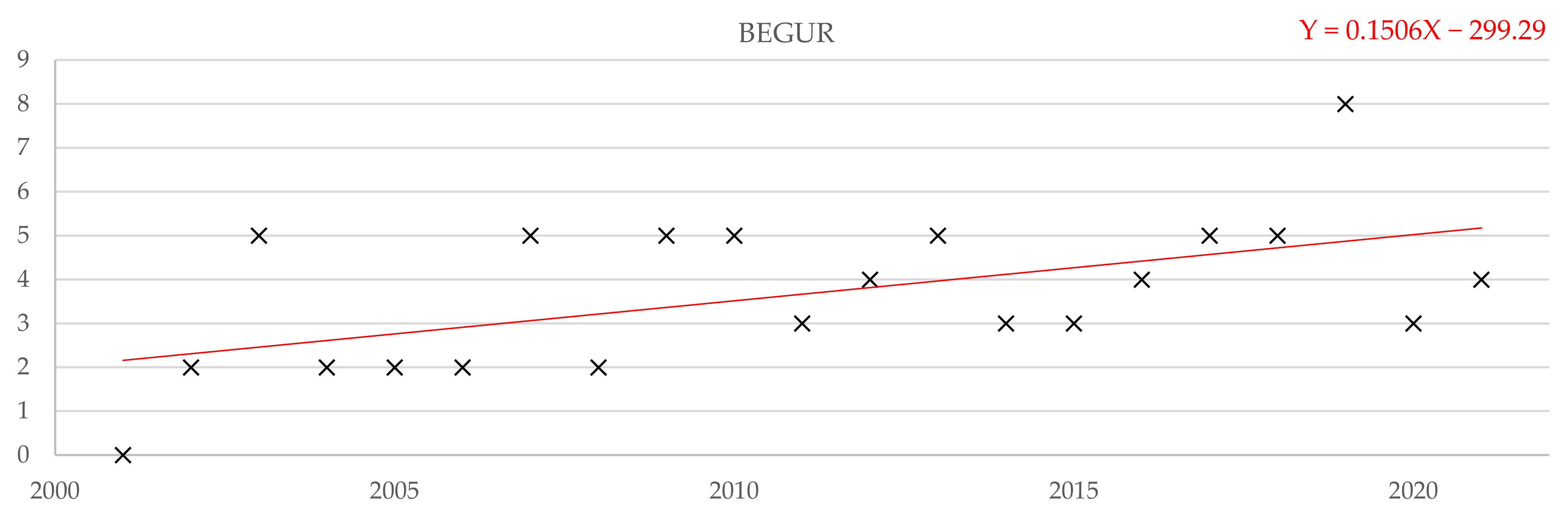
Number of times Hs has exceeded the threshold in Begur.

Figure 27.
Number of times Tp has exceeded the expected Tp in 100 years in the Gulf of Cadiz.

Figure 28.
Number of times Tp has exceeded the expected Tp in 100 years in Alboran.

Figure 29.
Number of times Tp has exceeded the expected Tp in 100 years in Gata.

Figure 30.
Number of times Tp has exceeded the expected Tp in 100 years in Mahon.

Figure 31.
Number of times Tp has exceeded the expected Tp in 100 years in Tarragona.

Figure 32.
Number of times Tp has exceeded the expected Tp in 100 years in Begur.

Figure 33.
Evolution of SL maxima in Tarifa.

Figure 34.
Evolution of SL maxima in Algeciras.

Figure 35.
Evolution of SL maxima in Almeria.

Figure 36.
Evolution of SL maxima in Valencia.

Figure 37.
Evolution of SL maxima in Mahon.

Figure 38.
Evolution of SL maxima in Sagunto.

Figure 39.
Evolution of SL maxima in Tarragona from 2011 to 2020.

Figure 40.
Evolution of SL maxima in Barcelona.

Figure 41.
Correlation of extremes in Almeria.

Figure 42.
Correlation of extremes in Valencia.

Figure 43.
Correlation of extremes in Mahon.

Figure 44.
Correlation of extremes in Sagunto.

Figure 45.
Correlation of extremes in Tarragona.

Figure 46.
Correlation of extremes in Barcelona.


Table 1.
List of buoys used in the study.
| Buoy | Longitude | Latitude | Depth | Records |
|---|---|---|---|---|
| 1. Gulf of Cadiz | 6.96° W | 36.49° N | 466 m | 1996–2022 |
| 2. Alborán | 5.03° W | 36.27° N | 585 m | 1997–2006 |
| 3. Cabo de Gata | 2.34° W | 36.57° N | 545 m | 1998–2022 |
| 4. Cabo de Palos | 0.31° W | 37.65° N | 242 m | 2006–2022 |
| 5. Valencia | 0.20° E | 39.51° N | 349 m | 2005–2022 |
| 6. Mahon | 4.42° E | 39.71° N | 310 m | 1993–2022 |
| 7. Tarragona | 1.47° E | 40.69° N | 685 m | 2004–2022 |
| 8. Begur | 3.65° E | 41.90° N | 1355 m | 2001–2022 |
Table 2.
List of tide gauges used in the study.
| Tide Gauge | Longitude | Latitude | Records |
|---|---|---|---|
| 1. Tarifa | 5.60° W | 36.01° N | 2009–2020 |
| 2. Algeciras | 5.40° W | 36.18° N | 2009–2020 |
| 3. Almeria | 2.48° W | 36.83° N | 2006–2020 |
| 4. Valencia | 0.31° W | 39.44° N | 1993–2020 |
| 5. Mahon | 4.27° E | 39.89° N | 2009–2020 |
| 6. Sagunto | 0.21° W | 39.63° N | 2007–2020 |
| 7. Tarragona | 1.21° E | 41.08° N | 2011–2020 |
| 8. Barcelona | 2.17° E | 41.34° N | 1993–2020 |
Table 3.
Summary of Hs and Tp extreme trends for each buoy.
| Buoy | Hs Slope | Tp Slope |
|---|---|---|
| Gulf of Cadiz | −4 × 10⁻⁶ | 1 × 10⁻⁵ |
| Alboran | 3 × 10⁻⁴ | 5 × 10⁻⁴ |
| Gata | 4 × 10⁻⁵ | 1 × 10⁻⁵ |
| Cabo de Palos | 1 × 10⁻⁵ | 1 × 10⁻⁴ |
| Valencia | −1 × 10⁻⁵ | 5 × 10⁻⁶ |
| Mahon | 1 × 10⁻⁴ | 1 × 10⁻⁴ |
| Tarragona | 5 × 10⁻⁵ | 1 × 10⁻⁴ |
| Begur | 3 × 10⁻⁵ | 8 × 10⁻⁵ |
Table 4.
Summary of SL slopes.
| Tide Gauge | SL Slope |
|---|---|
| 1. Tarifa | −1 × 10⁻⁴ |
| 2. Algeciras | 5 × 10⁻⁶ |
| 3. Almeria | −9 × 10⁻⁷ |
| 4. Valencia | 4 × 10⁻⁶ |
| 5. Mahon | 1 × 10⁻⁵ |
| 6. Sagunto | 1 × 10⁻⁵ |
| 7. Tarragona | 4 × 10⁻⁵ |
| 8. Barcelona | 1 × 10⁻⁵ |
Publisher’s Note: MDPI stays neutral with regard to jurisdictional claims in published maps and institutional affiliations. |
© 2022 by the authors. Licensee MDPI, Basel, Switzerland. This article is an open access article distributed under the terms and conditions of the Creative Commons Attribution (CC BY) license (https://creativecommons.org/licenses/by/4.0/).
Share and Cite
MDPI and ACS Style
Portillo Juan, N.; Negro Valdecantos, V.; del Campo, J.M. Analysis of Monthly Recorded Climate Extreme Events and Their Implications on the Spanish Mediterranean Coast. Water 2022, 14, 3453. https://doi.org/10.3390/w14213453
AMA Style
Portillo Juan N, Negro Valdecantos V, del Campo JM. Analysis of Monthly Recorded Climate Extreme Events and Their Implications on the Spanish Mediterranean Coast. Water. 2022; 14(21):3453. https://doi.org/10.3390/w14213453
Chicago/Turabian StylePortillo Juan, Nerea, Vicente Negro Valdecantos, and José María del Campo. 2022. "Analysis of Monthly Recorded Climate Extreme Events and Their Implications on the Spanish Mediterranean Coast" Water 14, no. 21: 3453. https://doi.org/10.3390/w14213453
Note that from the first issue of 2016, this journal uses article numbers instead of page numbers. See further details here.